A mean field stochastic theory for species-rich assembled communities

Abstract

A dynamical model of an ecological community is analyzed within a “mean-field approximation” in which one of the species interacts with the combination of all of the other species in the community. Within this approximation the model may be formulated as a master equation describing a one-step stochastic process. The stationary distribution is obtained in closed form and is shown to reduce to a logseries or lognormal distribution, depending on the values that the parameters describing the model take on. A hyperbolic relationship between the connectance of the matrix of interspecies interactions and the average number of species, exists for a range of parameter values. The time evolution of the model at short and intermediate times is analyzed using van Kampen’s approximation, which is valid when the number of individuals in the community is large. Good agreement with numerical simulations is found. The large time behavior, and the approach to the stationary state, is obtained by solving the equation for the generating function of the probability distribution. The analytical results which follow from the analysis are also in good agreement with direct simulations of the model.

PACS number(s): 05.40.-a, 05.10.Gg, 02.50.Ey, 87.23.Cc

I Introduction

The steady accumulation of data on all aspects of the very diverse ecosystems that exist on Earth has revealed a number of generic features [1]. Examples include (i) in species-rich ecosystems, the number of species, $S(n)$, with $n$ individuals following a power-law, $S(n)\approx n^{-\gamma}$, where $\gamma$ is close to one [1, 2], (ii) a relation between the number of species in the ecosystem, $S$, and the connectance, $C^{*}$ — defined as the number of predator-prey links between pairs of species divided by the total possible number of links — which has the hyperbolic form $C^{*}\approx S^{-1+\eta}$, with $\eta\in[0,1]$ [3], and (iii) other power-law distributions concerning the extinction of species, for instance, where the lifetime of species, $T$, appears to be well-described by the distribution $N(T)\approx T^{-\theta}$, with $\theta$ between 1.1 and 1.6 [4]. There is an urgent need for models of ecosystems to be developed which will allow the underlying mechanisms which lead to these regularities to be understood. These models need to be defined for an arbitrary number of species, have a set of rules specifying the interaction between pairs of species which is reasonably simple and based on general features such as the competition between species, and have a stochastic element to reflect the randomness of events which are inherent in real systems. In Ref [5] a model of this type was introduced in order to investigate the generic features outlined above. An analysis of the model was begun in that paper, where both numerical and analytical work showed predictions of the model to be in agreement with field data. Here we present a more detailed analysis of the model, using a variety of techniques, and compare the results of this analysis with that from real ecosystems. We begin by defining the model.

The ecosystem under study is taken to have $N$ individuals and $S$ possible species. It is modeled as a directed graph with the nodes labelled by $i=1,...,S$ representing the species, and the links representing the (predator-prey) interaction between the species at the two nodes being joined. This interaction is assumed to be given by a single real number, denoted by $\Omega_{ij}$ for the link to $j$ from $i$. Thus, the interaction between the species in the ecosystem is completely specified by the $S\times S$ real matrix $\bf\Omega$. Links from a node to itself are not allowed and therefore this matrix has zero entries on the diagonal. The antisymmetric matrix $S_{ij}\equiv\Omega_{ij}-\Omega_{ji}$ has a more direct interpretation as the “score” of species $i$ against species $j$:

• If $S_{ij}>0$, then $j$ acts as a resource for $i$.

• If $S_{ij}=0$, there is no interaction between $i$ and $j$.

• If $S_{ij}<0$, then $i$ acts as a resource for $j$.

Modelling multispecies ecosystems involving species-species interactions or connections of this type, has a long history [6]. Originally, population dynamics equations, such as the Lotka-Volterra equations, were written down for two species and then for many species. If one imagines studying the equations near to any fixed point that might exist, it is permissable to linearize about the fixed points, and the entire model is then specified by a single $S\times S$ matrix — the stability matrix. Whereas, for systems involving two species it might be useful to calculate this matrix in terms of the original parameters of the model, for systems of many species there are simply too many parameters and so the emphasis changed to trying to investigate general properties that such matrices might have. An obvious, but crude, assumption that the entries were random, was first investigated by May [7] who found that the connectivity of the matrix was important in determining its stability properties. Since then, this has remained a central issue in ecology [8], as has the study of the abstract theory of species connected by a complex network of interactions [9].

Having described the basic idea we will use in our approach, we now need to specify the interaction matrix $\bf\Omega$. Since, the connectivity seems to emerge as an important quantity in both theoretical and experimental studies we will assign a fixed conductivity $C$ to ${\bf\Omega}$, so that we may study how properties of the system change as $C$ is varied. Other than this, and the fact that the diagonal entries are zero, we will not impose any other restrictions on $\bf\Omega$. We now have to define the dynamics. The goal is to define a set of rules which is simple, but which builds up a complex model ecosystem, after a sufficiently long time, showing the non-trivial emergent behavior mentioned at the beginning of this section. We do this by assigning the (off-diagonal) entries of $\bf\Omega$, in a purely random way at $t=0$, and updating the system at discrete time steps as follows. At each time step:

• With probability $(1-\mu)$, pick two individuals at random. Suppose they belong to species $i$ and $j$ and that $S_{ij}\neq 0$. Replace the individual belonging to the species which has a negative score against the other species by a new individual of the more successful species. So, for example, if $S_{ij}>0$, the total number of individuals belonging to species $i$ goes up by one, and the total belonging to species $j$ goes down by one. If $S_{ij}=0$, no action is taken.

• With probability $\mu$, pick an individual at random. Replace it by another individual of any of the $S$ species.

These rules have an obvious interpretation. The first simply ensures that the most successful species, in the sense of the ones having the highest scores, grow at the expense of the less successful ones. However, if the dynamics consisted only of this rule, then eventually all species but one would go extinct. Therefore, a second rule has to be introduced in order to obtain a diverse ecosystem. The simplest choice is to violate the first rule occasionally, by giving even unsuccessful species an opportunity through purely random events. This is best not thought of as a mutation or speciation, but as an immigration event from an area outside the ecosystem under study.

We have not specified the initial distribution of the entries in $\bf\Omega$ and there is a certain amount of freedom regarding this choice. In our simulations we have chosen the $\Omega_{ij}\,(i\neq j)$ randomly from a uniform distribution on $[0,1]$, but any other choice is equally valid, since only the sign of $S_{ij}$ is important. Since the probability that $\Omega_{ij}=\Omega_{ji}\neq 0$ is vanishingly small, it is almost certain that if the condition $S_{ij}=0$ mentioned in rule 1 holds, then both $\Omega_{ij}$ and $\Omega_{ji}$ are zero, and species $i$ and $j$ are not connected by a predator-prey relationship. Since the probability of any matrix element being zero is $1-C$, the probability that both $\Omega_{ij}$ and $\Omega_{ji}$ are zero is $(1-C)^{2}$, and from what has been said above, the probability that $S_{ij}$ is non-zero is $C^{*}\equiv 1-(1-C)^{2}$.

For those simulations that start with no species in the system, a generalized $(S+1)\times(S+1)$ real matrix $\bf\Omega^{\prime}$ with an extra row and column denoted by 0 needs to be introduced. Then, if $S_{i0}>0$, empty space acts as a resource for $i$. If $S_{i0}<0$, then species $i$ fails to invade empty space. So, on average, the expected number of species that can actually invade empty space is $SC/2$ and the number of species in the pool that can never interact with empty space is $(1-C)S$.

What has been described above is a strongly interacting, stochastic multispecies model and as such is extremely difficult to study analytically. It is, however, relatively easy to simulate, given the straightforward nature of the algorithm described above, and we will discuss the results of extensive numerical studies in later sections of this paper. It would still be very useful to have some approximate treatment available which would, at the very least, help to suggest forms which could be use to fit the data and simulations. Fortunately, we can do much better than this. A mean field theory of the above model yields a master equation which can be analysed using a number of standard techniques. Much of the paper will be concerned with the derivation of these results and their subsequent interpretation.

The plan of the paper is as follows. In section II we derive the master equation within the mean field approximation and in section III we investigate the nature of the stationary state. The time-dependent properties are the subject of the next two sections: within a Gaussian approximation in section IV and a more general study in section V. We conclude with a summary of the work presented in the paper in section VI. There are two appendices: Appendix A and Appendix B contain technical details which are used to derive some of the results in sections III and V respectively.

II Master equation

In this section we will derive a master equation which approximately describes the complex dynamics introduced in section I. The key simplification is the use of a type of mean field theory. We focus on one of the $S$ species, which we shall call species $A$. The other $(S-1)$ species are no longer distinguished as separate species and are simply lumped together and denoted as species $B$. The $B$ species will be regarded as some kind of average species — a kind of effective background population — with which species $A$ interacts. There are various assumptions inherent in this approach. For instance, that the rate of reproduction is the same for all species, so that a typical species ($A$) can be picked out as representative. It does however, reduce the model to one in which just two species are interacting, namely $A$ and non-$A=B$. It is now relatively straightforward to derive a master equation which describes the dynamics of this process.

To derive this equation, first suppose that $\mu=0$ for simplicity. Then only rule 1 is in operation. In picking two individuals from a set of $N$ individuals of the $S$ species, the following situations arise: (a) both individuals belong to species $A$, (b) one belongs to $A$ and the other to $B$ and (c) both individuals belong to species $B$. In cases (a) and (c) there is no action taken under rule 1. The probability of case (b) occurring is the sum of the probability that first an $A$ is selected and then a $B$ and the probability that a $B$ is selected and then an $A$:

$$\frac{n}{N}\,\left(1-\frac{n-1}{N-1}\right)\ +\ \left(1-\frac{n}{N}\right)\,\left(\frac{n}{N-1}\right)\ =\frac{2n}{N}\,\left(\frac{N-n}{N-1}\right)\,,$$

where $n$ is the number of individuals of species $A$ in the ecosystem. We now have to focus on the quantity $S_{AB}$ in order to implement the rule. The probability that it is non-zero is $C^{*}$ and we would expect that, on average, half of the events the individual from species $A$ will have a higher score than the individual from species $B$ i.e. $S_{AB}<0$ and the other half of the events to have $S_{AB}<0$. Therefore, the probability that at each time step the number of species $A$ increases by one is

$$W(n+1|n)=C^{*}\frac{n}{N}\,\left(\frac{N-n}{N-1}\right)\,,$$

and the probability that at each time step the number of species $A$ decreases by one is

$$W(n-1|n)=C^{*}\frac{n}{N}\,\left(\frac{N-n}{N-1}\right)\,.$$

We will show shortly that this process leads to a stationary probability distribution which is non-zero only if $n=0$ or $n=N$, that is, only if either species $A$ dies out completely or dominates completely. The second rule ensures that some diversity is retained.

So suppose that we now include the second rule. The transition probabilities above have now to be multiplied by $(1-\mu)$ and those involving the second rule will involve a factor $\mu$. Specifically, the probability that the individual picked, when implementing the second rule, is replaced by an individual of a given species is $\mu/S$. If we ask that this given species is $A$, then since the probability that the individual picked belongs to species $B$ is $(1-n/N)$, the additional probability due to rule 2 that at each time step the number of species $A$ is increased by one is

$$\frac{\mu}{S}\,\left(1-\frac{n}{N}\right)\,.$$

Similarly, the probability that an individual is replaced by an individual of a different species is $\mu(S-1)/S$. Since the probability that the individual picked belongs to species $A$ is $n/N$, the additional probability that at each time step the number of species $A$ is decreased by one is

$$\frac{\mu}{S}\,(S-1)\,\frac{n}{N}\,.$$

Putting the two rules together, gives the one-step transition probabilities $g_{n}\equiv W(n+1|n)$ and $r_{n}\equiv W(n-1|n)$ as

$$g_{n}=C^{*}(1-\mu){n\over N}\left({N-n\over N-1}\right)+{\mu\over S}(1-{n\over N})\ ,$$ (1)

and

$$r_{n}=C^{*}(1-\mu){n\over N}\left({N-n\over N-1}\right)+{\mu\over S}(S-1){n\over N}\ .$$ (2)

We can now write down a master equation describing this one-step stochastic process [10, 11]. If $P(n,t)$ is the probability of species $A$ having $n$ individuals at time $t$, the master equation takes the form

$${dP(n,t)\over dt} = r_{n+1}P(n+1,t)+g_{n-1}P(n-1,t)$$ (3)

$$- (r_{n}+g_{n})P(n,t)\,.$$ (4)

Equation (4) is only valid for values of $n$ not on the boundary (i.e. for $n\neq 0$ and $n\neq N$); for these values special equations have to be written reflecting the fact that no transitions out of the region $[0,N]$ are allowed. However, from (1) and (2) we see that $g_{N}=0$ and $r_{0}=0$, and if additionally we define $r_{N+1}=0$ and $g_{-1}=0$, then (4) holds for all $n=0,1,...,N$. To completely specify the system we also need to give an initial condition, which will typically have the form $P(n,0)=\delta_{n,m}$ for some non-negative integer $m$.

We will end this section by determining the stationary probability distribution, $P_{s}(n)$. Setting $dP(n)/dt=0$, one obtains

$$r_{n+1}P_{s}(n+1)-g_{n}P_{s}(n)=r_{n}P_{s}(n)-g_{n-1}P_{s}(n-1)\,.$$ (5)

This is true for all $n$, which implies that $r_{n}P_{s}(n)-g_{n-1}P_{s}(n-1)=J$, where $J$ is a constant. Applying the boundary condition at $n=0$, we find that $J=0$ and therefore

$$r_{n}P_{s}(n)=g_{n-1}P_{s}(n-1)\ ;\ n=0,1,...,N\,.$$ (6)

If $\mu\neq 0$, then $r_{n}\neq 0$ for all $n$ such that $0<n\leq N$, and therefore

$$P_{s}(n)=\frac{g_{n-1}\,g_{n-2}...\,g_{0}}{r_{n}\,r_{n-1}...\,r_{1}}P_{s}(0)\ ;\ n=1,...,N\,.$$ (7)

The constant $P_{s}(0)$ can be determined from the normalization condition

$$\sum_{n=0}^{N}P_{s}(n)=P_{s}(0)+\sum_{n>0}P_{s}(n)=1\,:$$ (8)

$$(P_{s}(0))^{-1}=1+\sum_{n=1}^{N}\frac{g_{n-1}\,g_{n-2}...\,g_{0}}{r_{n}\,r_{n-1}...\,r_{1}}\,.$$ (9)

At this point it is convenient to introduce a set of combinations of the constants of the model which will appear frequently in the analysis. These are:

$$\mu^{*}=\mu/[(1-\mu)SC^{*}]\ \ ,\ \ \lambda^{*}=\mu^{*}(N-1)$$

$${\rm and}\ \ \nu^{*}=N+\mu^{*}(N-1)(S-1)\,.$$ (10)

The transition probabilities (1) and (2) may now be written in the more compact form

$$g_{n} = \frac{C^{*}(1-\mu)}{N(N-1)}\,(N-n)(\lambda^{*}+n)\ \ {\rm and}$$ (11)

$$r_{n} = \frac{C^{*}(1-\mu)}{N(N-1)}\,n(\nu^{*}-n)\,.$$ (13)

Substituting (13) into (9) gives

$$(P_{s}(0))^{-1} = \sum_{n=0}^{N}{N\choose n}{\Gamma(n+\lambda^{*})\over\Gamma(\lambda^{*})}{\Gamma(\nu^{*}-n)\over\Gamma(\nu^{*})}$$ (14)

$$= \sum_{n=0}^{N}{N\choose n}(-1)^{n}{\Gamma(n+\lambda^{*})\over\Gamma(\lambda^{*})}{\Gamma(1-\nu^{*})\over\Gamma(n+1-\nu^{*})}\ .$$ (16)

This sum takes the form of a Jacobi polynomial $P_{N}^{(\alpha,\beta)}(x)$ [12], with $\alpha=-\nu^{*}$, $\beta=\lambda^{*}+\nu^{*}-(N+1)$ and $x=-1$, which can itself be expressed in terms of gamma functions for this value of $x$. So using (7) we find

$$P_{s}(n)={N\choose n}{\Gamma(n+\lambda^{*})\over\Gamma(\lambda^{*})}{\Gamma(\nu^{*}-n)\over\Gamma(\nu^{*}-N)}{\Gamma(\lambda^{*}+\nu^{*}-N)\over\Gamma(\lambda^{*}+\nu^{*})}\ .$$ (17)

In various intermediate expressions we have assumed that $\nu^{*}$ is not an integer, but this final result is well defined for all meaningful ranges of the parameters, since from (10) we can see that $\nu^{*}>N$ and $\lambda^{*}>0$. Moreover $P_{s}(n)>0$ for all $n=0,1,...,N$ and $\sum_{n}P_{s}(n)=1$ by construction. By introducing the beta function $\beta(p,q)=\Gamma(p)\Gamma(q)/\Gamma(p+q)$, the stationary, normalized solution can be written in the more compact form

$$P_{s}(n)={N\choose n}{\beta(n+\lambda^{*},\nu^{*}-n)\over\beta(\lambda^{*},\nu^{*}-N)}\ .$$ (18)

Finally, if $\mu=0$, $r_{N}=0$, so (7) no longer holds for $n=N$. Using the result that $g_{0}=0$ in this case, one finds that $P_{s}(n)=0$ for $n=1,...,N-1$. By normalization we can write $P_{s}(0)={\cal C}$ and $P_{s}(N)=1-{\cal C}$, where $\cal C$ is a constant. So, as mentioned earlier, either species $A$ is the only surviving species or it goes extinct. In other words, in the stationary state only one species survives. Since all species are assumed identical, it follows that when $\mu=0$

$$P_{s}(0)=\frac{1}{S}\ \ ;\ P_{s}(N)=1-\frac{1}{S}\ \ ;\ P_{s}(n)=0\ {\rm for}\ 0<n<N\,.$$ (19)

Although we have obtained the exact solution for the stationary distribution (17) in terms of nothing more complicated than gamma functions, we still need to simplify it if we are to compare the result with data. In the next section, we will derive simpler forms for the stationary probability distribution which are valid in different regions of the parameter space of the model, and compare these with simulations.

III stationary state

We have so far been discussing the stationary state from the point of view of a time-independent solution of the master equation. But let us now ask the question in a biological context: are ecological communities in stable equilibria? Although is obvious that environmental variability and chance have a great impact on ecosystems, some well-defined, time-independent, patterns arise when natural ecosystems are observed. The model we have introduced reaches a well-established dynamic stationary state which allows us to study some of these patterns. A particular example of interest is the way that individuals are distributed among species. In any island where colonization from the mainland and local extinction take place, a dynamical equilibrium between these two processes is reached [13]. In these situations our model applies and can help to understand the patterns observed.

Highly diverse ecological communities are formed when a large number of different species are present. The estimation and characterization of such biological diversity is not only a central issue in theoretical ecology, but also a question of practical concern for nature reserve design and conservation biology in general. In any ecological community species vary considerably in the number of individuals that belong to that species. Some species are very difficult to find because they are very rare. Some of them are extremely common. How are individuals distributed among species? What factors affect this distribution? The classic way of studying this topic is by means of species abundance relations — the “relations between abundance and the number of species possessing that abundance” [14]. Different types of species abundance relations have been used to fit to real species abundance data. Some of them have been justified on theoretical grounds (see [1] for a review). One of the most widely used species abundance distribution was first discussed by Fisher, Corbet and Williams in 1943 [15]. The distribution is defined by two parameters $x$ and $\alpha$:

$$S(n)=\frac{\alpha x^{n}}{n}\,,$$ (20)

where $S(n)$ is the number of species having $n$ individuals. Since (20) summed over $n$ gives a logarithm, this is known as the logseries distribution. It is very common as a sampling distribution in the ecological literature, although it has also been derived on theoretical grounds [16, 17].

The abundance distribution that has received more attention from ecologists, however, was introduced by Preston in one of the most influential papers on ecological theory [18, 19]. As May remarks “theory and observation points to its ubiquity once $S\gg 1$, when relative abundances must be governed by the conjunction of a variety of independent factors” [14]. The distribution is the lognormal distribution, so called because the logarithm of species abundances is normally distributed:

$$S(R)=S(n_{0})\exp(-\frac{R^{2}}{2\rho^{2}})\,,$$ (21)

where, following Preston’s definitions, $R=\log_{2}(n/n_{0})$ is a logarithmic measure of the abundance in relation to $n_{0}$ — the abundance value where the distribution has its maximum. So, $S(R)dR$ is the number of species having their logarithmic relative abundance between $R$ and $R+dR$. Notice that both equations (20) and (21) must be divided by the total number of species to be properly understood as estimations of the probability distribution function.

In this section we want to compare the exact result for $P_{s}(n)$ with these two distributions — the most widely used abundance distributions in the ecological arena. We will derive simpler forms for the stationary probability distribution which are valid in different regions of the parameter space of the model, and compare these with simulations of the original model (that is, without making the mean-field approximation). Lognormal and logseries distributions will naturally emerge for different well-defined immigration regimes. In a forthcoming paper we will analyse a large quantity of species abundance data from different ecological communities in detail.

We begin by discussing one situation in which the logseries distribution occurs. It turns out to be convenient to rewrite the result (17) for $P_{s}(n)$ by breaking it down into three separate parts:

$$P_{s}(n)={\cal F}_{1}(n)\,{\cal F}_{2}(N)\,{\cal F}_{3}(n,N)\,,$$ (22)

where

$${\cal F}_{1}(n) = \frac{\Gamma(n+\lambda^{*})}{n!\,\Gamma(\lambda^{*})},$$ (23)

$${\cal F}_{2}(N) = \frac{\Gamma(\nu^{*})}{\Gamma(\lambda^{*}+\nu^{*})}\frac{\Gamma([\nu^{*}-N]+\lambda^{*})}{\Gamma(\nu^{*}-N)}\ \ \left(=P_{s}(0)\right),$$ (25)

$${\rm and}\ \ {\cal F}_{3}(n,N) = \frac{N!}{(N-n)!}\frac{\Gamma(\nu^{*}-n)}{\Gamma(\nu^{*})}\,.$$ (27)

We will now give a simpler form for each of these expressions, being careful to state the range of validity of our approximations in each case. Details of the derivation of these results is given in Appendix A. The non-trivial behavior occurs for relatively small values of $n$, so in what follows we will only be interested in values of $n$ up to $n_{\rm max}$, where $n_{\rm max}\ll N$ and $N\gg 1$. We will also suppose that there are many possible species: $S\gg 1$.

From Eqns. (A8) and (A6) we have that

$${\cal F}_{1}(n)\approx\frac{\lambda^{*}}{n}\ \ ;\ n\gtrsim 1\ ;\ \lambda^{*}\ll\frac{1}{\ln n_{\rm max}}$$ (28)

and

$${\cal F}_{3}(n,N)\approx\exp{\left(-n\lambda^{*}S/N\right)}\ \ ;\ \lambda^{*}S\ll N\ \ ;\ \lambda^{*}S\ll\left(\frac{N}{n_{\rm max}}\right)^{2}\,.$$ (29)

Therefore (22)-(29) give

$$P_{s}(n)={\cal K}n^{-1}\exp(-n\mu^{*}S)\ ,$$ (30)

where ${\cal K}\equiv\lambda^{*}P_{s}(0)$. This is the logseries (20) with $x=e^{-\mu^{*}S}$ and expressed as the fraction of species represented by $n$ individuals in the steady state. Note that (20), by contrast, gives the absolute number of species with a given abundance $n$.

Since $S<N$, the condition $\lambda^{*}S\ll N$ is redundant when the stronger condition $\lambda^{*}\ll 1/\ln n_{\rm max}$ is imposed. Therefore, (30) holds when

$$1\lesssim n\leq n_{\rm max}\ll\frac{N}{\sqrt{\lambda^{*}S}}\ \ \ {\rm and}\ \ \ \lambda^{*}\ll\frac{1}{\ln n_{\rm max}}\,.$$ (31)

To find an approximate form for ${\cal K}$, we use (A12) which gives an approximate form for $P_{s}(0)={\cal F}_{2}(N)$. Under the very reasonable conditions that $\lambda^{*}$ is much less than $N/S$, $\sqrt{N}$ and $S$, but with $\lambda^{*}S\gtrsim 1$, we find

$${\cal K}\approx\lambda^{*}\,(\mu^{*}S)^{\lambda^{*}}\,.$$ (32)

Fig 1 shows the results of different simulations which have been performed for increasing values of the immigration parameter. In order to calculate the species relative abundance distribution an ensemble average has been performed. For each plot a collection of 2000 replicas has been simulated. For each replica the probability distribution $P(n,t)$ has been calculated after 500000 simulation time steps. In Fig 1, the $\lambda^{*}$ values increase from $0.033$ when $\mu=0.001$ to $3.3$ when $\mu=0.1$. The last three plots do not show such a good match with the logseries approximation as the first three. Even in the upper three plots, where there appears to be a good fit with the logseries, we would only expect a complete match for $1<n\lesssim 10$. From (31), we should bear in mind that this is only expected to be true as long as $\lambda^{*}\ll 1/\ln n_{\rm max}$. For instance, $\lambda^{*}=0.22$ for $\mu=10^{-2}$ (for the parameter set $N=5000$, $S=300$ and $C=0.5$) and $1/\ln n_{\rm max}$ is $0.434$ when $n_{\rm max}=10$.

FIG. 1.: Stationary probability distribution $P_{s}(n)$ obtained from the exact solution (18) (solid line) and the logseries approximation (30) (dotted line), with the simplest form for the multiplicative factor $\cal{K}$ (32), for different immigration values. In each plot the species relative abundance distribution resulting from the individual based model is also shown (noisy solid line).

In Fig 2 two simulation results are displayed. The stationary solution is also shown in both cases for comparison purposes. The stationary solution is calculated numerically either by direct application of equation (17), as has been done in Fig 1, or by means of an algorithm that can find the stationary probability distribution of any one-step stochastic process if it exists, as in Fig 2. This algorithm is based on the subroutine TRIDAG [20]. To describe it, we first write the master equation (4) in the more general form:

$${dP(n,t)\over dt}=\sum_{n\neq n^{\prime}}\,{\cal W}_{n,n^{\prime}}\,P(n^{\prime},t)-\sum_{n\neq n^{\prime}}\,{\cal W}_{n^{\prime},n}\,P(n,t)\,,$$ (33)

where $r_{n}={\cal W}_{n-1,n}$ and $g_{n}={\cal W}_{n+1,n}$. If we now introduce $W_{n,n^{\prime}}=(1-\delta_{n,n^{\prime}})\,{\cal W}_{n,n^{\prime}}-\delta_{n,n^{\prime}}\,\sum_{n^{\prime\prime}\neq n}{\cal W}_{n^{\prime\prime},n}$ and the vector $\vec{P}(t)=(P(1,t),\ldots,P(N,t))$, (33) may be written in the matrix form

$$\frac{d}{dt}{\vec{P}}=W\cdot{\vec{P}}\,.$$ (34)

Finding the stationary stationary distribution $P_{s}(n)$ — the vector ${\vec{P}}_{s}=(P_{s}(0),\ldots,P_{s}(N))$ — is then equivalent to solving a system of $N+1$ linear equations $W\cdot{\vec{P}}_{s}=0$ in $N+1$ unknowns: $P_{s}(n),\;n=0,\ldots,N$. In any one-step stochastic process the matrix $W$ is tridiagonal. Our algorithm takes advantage of this feature to solve the system.

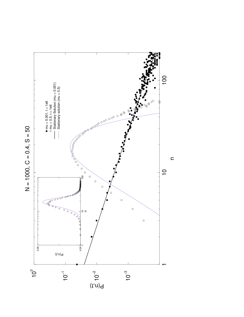
FIG. 2.: Abundance distributions for two individual-based simulations are presented for two extreme values of the immigration parameter. Time is measured in simulation time units. The stationary distribution $P_{s}(n)$ is also shown in both cases.

Another quantity which is useful in comparing model predictions to data is the average number of species in the stationary state, which we denote by $\langle S\rangle$. Let $P_{i}(n)$ be the probability that there are $n$ individuals of species $i$ in the ecosystem. Therefore the probability that there is at least one individual of species $i$ is $1-P_{i}(0)$ and so the average number of species is $\langle S\rangle=\sum_{i}(1-P_{i}(0))$. Within the mean field approximation $P_{i}(0)$ is the same for all species $i$: $P_{i}(0)=P_{s}(0)$ (the subscript $s$ denotes “stationary”, as before), so that

$$\langle S\rangle=\sum^{S}_{i=1}(1-P_{s}(0))=(1-P_{s}(0))S\,.$$ (35)

Under the conditions $\lambda^{*}S\gtrsim 1$, $\lambda^{*}\ll\epsilon$ and $|\ln C^{*}|\ll|\ln\mu|$, we show in Appendix A that (see eq. (A17))

$$\langle S\rangle\sim\left(C^{*}\right)^{-1+\epsilon}\,,$$ (36)

where $\epsilon^{-1}\approx|\ln\mu|$ (see Fig 3). Inverting this relationship gives $C^{*}\sim\langle S\rangle^{-1+\eta}$ with $\eta=\epsilon/(\epsilon-1)$. The condition $\lambda^{*}S\gtrsim 1$ is essentially equivalent to $\mu N\gtrsim 1$ (for a connectance that is not too small). For systems of interest $N$ is very large, and hence $\mu$ must typically be very small if the hyperbolic relation (36) is to hold. Such a tiny value of $\mu$ means that $\epsilon$ and hence $\eta$, will be close to zero. The form of the relationship between $C^{*}$ and $\langle S\rangle$ when the immigration parameter has a larger value will be discussed elsewhere.

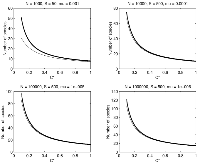
FIG. 3.: Species-connectivity relationship for different parameter values. The expected number of species in the system in the steady state is shown plotted against the connectance $C^{*}$. Notice that as long as $\lambda^{*}S$ remains close to but slightly greater than 1, a very good agreement is shown between the exact form (35) (single line in the plot) and the hyperbolic species-connectivity relationship (36) (double line).

In Fig 4 the species-connectivity relationship calculated from the individual modelling approach is shown. After carrying out 600000 simulation steps, a 1000 ensemble average was calculated for each connectivity value. The initial condition is the empty system. Although our mean field approximation captures the essentials of the hyperbolic-like behavior of the species-connectivity relationship, there is a systematic deviation from the mean field prediction in the simulated curves.

FIG. 4.: Species-connectivity relationship. Two simulations are presented. Standard deviations from the ensemble average value are shown. In the plot on the left, $\lambda^{*}S\simeq 25$ — too high a value to fit the approximation given by (36). So in this case the only plotted curve is the exact mean field relation (35). In the plot on the right, conditions needed to apply (36) are quite well fulfilled and two curves are plotted: the exact mean field relation (solid line) and the approximation (dotted line).

To sum up, the exact solution given in (18) admits a logseries representation for low immigration regimes. For these low immigration values a hyperbolic-like relation is also observed between the mean number of species in the stationary state and the connectivity level given by the trophic relationships pre-defined in the community matrix, $\bf\Omega$. We will now argue that the exact stationary distribution probability is also very well approximated by a lognormal distribution for intermediate to high immigration regimes as shown in Figs 5 and 2.

The idea behind the analysis we will present, is to find at which values of $n$, if any, $P_{s}(n)$ has a maximum. We then expand $P_{s}(n)$ about this maximum to see to what extent this function can be analytically described by a lognormal distribution.

First of all, from Fig 5, we can see that $P_{s}(n)$ may admit a Gaussian representation for some parameter values. So let us look at this case first, before discussing the lognormal. To investigate for what parameter values this may occur, we first find the position of the maximum of $P_{s}(n)$. It is more convenient to consider $\ln P_{s}(n)$ rather than $P_{s}(n)$. From (17), we get:

$$\frac{d\ln P_{s}(n)}{dn}=-\psi(n+1)+\psi(n+\lambda^{*})-\psi(\nu^{*}-n)+\psi(N-n+1)\,,$$ (37)

where

$$\psi(z)\equiv\frac{d\ln\Gamma(z)}{dz}\,.$$

Setting (37) equal to zero gives the maximum value of $P_{s}(n)$ at $n=\hat{n}$. If all arguments of the psi-functions can be considered to be large enough, which is true if $n\ll N$ but reasonably large (e.g. $n\gtrsim 100$), these functions can be approximated using $\psi(z)\sim\ln z$ [12]. So,

$$\frac{d\ln P_{s}(n)}{dn}\approx-\ln(n+1)+\ln(n+\lambda^{*})-\ln(\nu^{*}-n)+\ln(N-n+1)=0,$$ (38)

from which one finds that the maximum is given by:

$$\hat{n}=\frac{(N+2)(\lambda^{*}-1)}{\lambda^{*}S-2}-1\,.$$ (39)

From (39) we can see that if $\lambda^{*}S<2$ (very low immigration regimes), the numerator and denominator are both negative and a maximum exists. However it is inadmissible, since it violates the condition $\hat{n}\ll N$. Therefore, a necessary condition for the existence of a maximum, $\hat{n}$, is that $\lambda^{*}>1$.

Now, we perform a Taylor expansion of (17) about $\hat{n}$ to quadratic order. If $n=\hat{n}+\delta n$, then for $\delta n$ small:

$$\ln P_{s}(n)=\ln P_{s}(\hat{n})+\frac{1}{2}\left.\frac{d^{2}\ln P_{s}(n)}{dn^{2}}\right|_{n=\hat{n}}(n-\hat{n})^{2}+O(\delta n)^{3}\,.$$

Since $\hat{n}$ is a maximum, $d^{2}\ln P_{s}(n)/dn^{2}|_{n=\hat{n}}<0$, and so we set this equal to $-1/\sigma^{2}$. Then ignoring the $O(\delta n)^{3}$ terms and exponentiating gives

$$P_{s}(n)=P_{s}(\hat{n})\exp(-\frac{(n-\hat{n})^{2}}{2\sigma^{2}})\,.$$ (40)

Under this approximation ($n\ll N$, but reasonably large) it is not very difficult to derive an analytical expression for the variance:

$$\sigma=\frac{\sqrt{\hat{n}^{2}+(\lambda^{*}+1)\hat{n}+\lambda^{*}}}{\sqrt{\lambda^{*}-1}}\,.$$ (41)

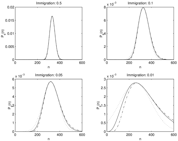
FIG. 5.: Lognormal approximation (the long-dashed curves) for the exact stationary solution (18) (solid line curves). The parameter values that have been used are $N=100000$, $S=300$ and $C=0.5$. The Gaussian approximation (dotted curves) is also shown.

Since the Gaussian distribution is completely specified by its first two cumulants, fixing $\hat{n}$ and $\sigma$ given by (39) and (41) respectively, determines the entire curve. The dotted lines in Fig 5 show this curve i.e. (40) with the two parameters fixed by (39) and (41). The upper two plots show very good agreement with the exact mean field approximation; in the lower two plots the agreement is not so good.

To approximate the exact stationary solution as a lognormal distribution (21), we will proceed in a similar way. Equation (21) can also be written dividing by the total number of species as:

$${\cal P}(R)={\cal N}\exp(-\frac{R^{2}}{2\rho^{2}})={\cal N}\exp\left(-\frac{(\ln n-\ln n_{0})^{2}}{2\sigma^{2}}\right)\,,$$ (42)

where $\sigma=\rho\ln 2$ and where ${\cal N}$ is a normalization constant to be determined. So let us express the solution (17) as a function of $\ln n$ instead of $n$. After this change of variable a new, equivalent, probability distribution function arises, ${\cal P}(x)$, where $x=\ln n$, that has to satisfy $P_{s}(n)dn={\cal P}_{s}(x)dx$, or, in other words,

$${\cal P}_{s}(x)=\frac{dn}{dx}\,P_{s}(n)=n\,P_{s}(n)\,,$$ (43)

which implies that

$$\frac{d\ln{\cal P}_{s}(x)}{dx}=1+e^{x}\left[-\psi(e^{x}+1)+\psi(e^{x}+\lambda^{*})-\psi(\nu^{*}-e^{x})+\psi(N-e^{x}+1)\right]\,.$$ (44)

Setting equation (44) equal to zero, and using $x=\ln n$, we obtain the position of maximum by finding the zero, $n_{0}$, of the equation

$$\left[\psi(n+1)-\psi(n+\lambda^{*})+\psi(\nu^{*}-n)-\psi(N-n+1)\right]=\frac{1}{n}\,.$$

In exactly the same way as for the Gaussian case, we can write the Taylor expansion up to second order:

$$\ln{\cal P}_{s}(x)=\ln{\cal P}_{s}(x_{0})-\frac{1}{2\sigma^{2}}(x-x_{0})^{2}\,$$

or, equivalently

$${\cal P}_{s}(x)={\cal P}_{s}(x_{0})\exp(-\frac{(\ln n-\ln n_{0})^{2}}{2\sigma^{2}})$$

where $x_{0}=\ln n_{0}$. Finally, using equation (43), we get a lognormal expression for the mean field solution:

$$P_{s}(n)=\frac{K}{n}\exp(-\frac{(\ln n-\ln n_{0})^{2}}{2\sigma^{2}})$$ (45)

where $K=n_{0}P_{s}(n_{0})$.

The evaluation of the second derivative at $x=x_{0}$ allows us to fix a value for the variance $\sigma^{2}$:

$$\frac{1}{\sigma^{2}}=1-(n_{0})^{2}\left[-\psi^{\prime}(n_{0}+1)+\psi^{\prime}(n_{0}+\lambda^{*})+\psi^{\prime}(\nu^{*}-n_{0})-\psi^{\prime}(N-n_{0}+1)\right]\,.$$

Although in this case there is no way to derive a simple, yet sufficiently general, analytical expression for the maximum $n_{0}$ and the variance $\sigma^{2}$, in Fig 5 we have used the asymptotic series expansion for $\psi(z)$ [12] to calculate numerically both quantities. Once again, since the lognormal distribution is completely specified by $n_{0}$ and $\sigma^{2}$, fixing these fixes the entire curve. The figure shows that the lognormal approximation matches the exact solution well for intermediate to high immigration regimes. We also note that, in general, the lognormal is a better fit to the exact solution than the Gaussian.

Lognormal and logseries distributions have been used by ecologists to fit real abundance data for years [15, 18, 19, 2, 1, 21]. Our results show that it is possible for both distributions to stem from the same general ecological process under different immigration regimes. If, for instance, we counted species abundances in a small area within a wood, the lognormal distribution would probably arise since that area is no doubt weakly isolated from the rest of the wood by external immigration. The same experiment performed in a rather isolated area might be expected to give rise to an empirical relative abundance distribution well fitted by a logseries function.

Finally, in this section we calculate the diversity, $H$, of the ecosystem (also called the Shannon entropy) for our model in the stationary state. It is defined by

$$H=-\sum_{i=1}^{S}p_{i}\ln p_{i}\,,$$ (46)

where $p_{i}$ is the probability that an individual selected at random from the system belongs to species $i$ [1]. Clearly, $p_{i}=n_{i}/N$, where $n_{i}$ is the number of individuals of species $i$ in the stationary state. On the other hand, within our mean field approach, the quantity which we can calculate is $P_{s}(n)$ — the probability that a typical species will have $n$ individuals in the system when it is in the stationary state. Since the number of species with $n$ individuals in the system is just $SP_{s}(n)$, we may express (46) within our approximation as

$$H=-\sum_{n}SP_{s}(n)\,(n/N)\,\ln\left(n/N\right)\,.$$ (47)

Multiplying (4) by $n$ and summing, it is easy to find that $\langle n\rangle=N/S$ in the stationary state. Using this result we have

$$H = -\frac{S}{N}\sum_{n}P_{s}(n)\,n\left(\ln n-\ln N\right)$$ (48)

$$= -\frac{S}{N}\left\{\langle n\ln n\rangle-\langle n\rangle\,\ln N\right\}$$ (49)

$$= \,\ln N\,-\,\frac{S}{N}\langle n\ln n\rangle\,.$$ (50)

Therefore we only need to evaluate $\langle n\ln n\rangle$ in the stationary state to find $H$. Fig 6 shows the result of performing this evaluation using the stationary probability distribution $P_{s}(n)$, for increasing values of the immigration parameter $\mu$. For comparison purposes, direct computation of the average number of species and the average entropy for 1000 replicas of the model and its standard deviation is shown. It can be seen that for relatively low immigration rates the system tends to be saturated admitting as many species as possible. As immigration increases, the Shannon entropy grows steeper than the number of species does, meaning that immigration tends to equalize the number of individuals of different species first, rather than increase the actual number of species in the system.

In Figs 4 and 6 it can be seen that ensemble average curves for the expected number of species in the stationary state deviate systematically from the mean field approximation that we have implemented through the master equation (4), even though they show the same qualitative behaviour. The explanation for this slight disagreement comes from the way we are estimating the probability of an effective interaction within the system. When transition probabilities are discussed (Eqns. (1) and (2)), the probability of interaction is split into a product of the probability of picking two potential interacting individuals multiplied by the probability of having an actual link between the species they belong to. However, these two events are not independent. The assumption of independence is just an approximation that allows us to simplify the system and get some insight into the dynamical processes that take place during simulations. In particular, for any parameter choice, the individual based model has more interactions than expected and cannot maintain the same number of species as predicted by our mean field approximation.

FIG. 6.: The expected value for the number of species and the Shannon entropy as a measure of diversity is computed at the steady state using the stationary distribution (18) for increasing values of immigration parameter. Ensemble averages of these two quantities are also shown for increasing discrete values of the same parameter. 1000 replicas of the model have been simulated. Values for the number of species and Shannon entropy have been recorded after 500000 simulation time steps, when the system has reached the stationary state.

IV time dependence

What can our model say about the assembly of an ecological community? Whenever species colonize a new island or any empty space, a new community builds up from scratch. The process that takes place is called succession by ecologists. The assembly of an ecological community has been studied both from the theoretical and empirical point of view. Many patterns have been found during the process of ecological succession (see [22] for a review). For instance, the number of species grows in a particular way that depends on the immigration from a biogeographical species pool. If our model is to make any prediction about succession, simulation time must have a direct meaning in terms of physical time. In our model the only connection to physical time comes from the immigration parameter, but the model has in fact two time scales. The external one is defined by the flux of individuals from the biogeographical pool and the internal one is defined by the flux of individuals (birth-death process) as a consequence of the internal dynamics (pairwise random encounters) within the system. Our immigration parameter captures the relative importance of these two different temporal processes.

Therefore, having investigated the properties of the stationary state in the last section, we now move on to the study of the time evolution of the system within the mean-field approximation. The master equation (4) has transition probabilities $g_{n}$ and $r_{n}$ which are non-linear in $n$, so that an exact solution for the time-dependent behavior is not possible. However, since in the problem of interest $N$ is very large, the possibility of performing a large-$N$ analysis suggests itself. In this section we will describe the application of such an analysis — specifically van Kampen’s large-$N$ method [10] — to our model. This method has a number of attractive features, for instance, the macroscopic (i.e. deterministic) equation emerges naturally from the stochastic equation as a leading order effect in $N$, with the next to leading order giving the Gaussian broadening of $P(n,t)$ about this average motion. The method is clearly presented in [10], so we will only give a brief outline of the general idea and stress the application to the model of interest in this paper.

If we take the initial condition on (4) to be $P(n,0)=\delta_{n,m}$, we would expect, at early times at least, $P(n,t)$ to have a sharp peak at some value of $n$ (of order $N$), with a width of order $N.N^{-1/2}=N^{1/2}$. It is therefore, natural to transform from the stochastic variable $n$ to the stochastic variable $\xi$ by writing

$$n=N\phi(t)+N^{1/2}\xi$$ (51)

where $\phi(t)$ is some unknown macroscopic function which will have to be chosen to follow the peak in time. A new probability distribution $\Pi$ is defined by $P(n,t)=\Pi(\xi,t)$, which implies that

$$\dot{P}=\frac{\partial\Pi}{\partial t}-N^{1/2}\,\frac{d\phi}{dt}\,\frac{\partial\Pi}{\partial\xi}\,.$$ (52)

The master equation (4) may be written

$$\dot{P}_{n}=\left({\cal E}-1\right)r_{n}P_{n}+\left({\cal E}^{-1}-1\right)g_{n}P_{n}\,,$$ (53)

where ${\cal E}$ (${\cal E}^{-1}$) is an operator which changes $n$ into $n+1$ ($n-1$), e.g. if $f_{n}$ is an arbitrary function of $n$, then ${\cal E}f_{n}=f_{n+1}$. In terms of $\xi$:

$${\cal E}^{\pm 1}=1\pm N^{-1/2}\,\frac{\partial\ }{\partial\xi}+\frac{1}{2\,!}\,N^{-1}\,\frac{\partial^{2}}{\partial\xi^{2}}+\ldots\,.$$ (54)

Using (51)-(54) the original master equation for $P(n,t)$ can be rewritten as an equation for $\Pi(\xi,t)$. By rescaling the time according to $\tau=t/N$, a hierarchy of equations can be derived by identifying terms order by order in powers of $N^{-1/2}$. The first two of these are:

$$\frac{d\phi}{d\tau}=\alpha_{1,0}(\phi)$$ (55)

and

$$\frac{\partial\Pi}{\partial\tau}=-\alpha^{\prime}_{1,0}(\phi)\,\frac{\partial\ }{\partial\xi}\left(\xi\Pi\right)+\frac{1}{2}\,\alpha_{2,0}(\phi)\,\frac{\partial^{2}\Pi}{\partial\xi^{2}}\,,$$ (56)

where

$$\alpha_{1,0}(\phi) = \frac{\mu}{S}-\mu\phi$$ (57)

$$\alpha_{2,0}(\phi) = 2C^{*}(1-\mu)\phi(1-\phi)+\frac{\mu}{S}+\frac{\mu}{S}\,(S-2)\phi\,.$$ (58)

The first equation (55) is the macroscopic equation for $\phi(\tau)$. It is easily solved to give

$$\phi(\tau)=\phi(0)e^{-\mu\tau}+\frac{1}{S}\,(1-e^{-\mu\tau})\,.$$ (59)

Initially we ask that $\xi(0)=0$, which means that $\phi(0)=n(0)/N=m/N$. Going back to the $t$ variable gives

$$\phi(t)=\frac{m}{N}\,e^{-\mu t/N}+\frac{1}{S}\,(1-e^{-\mu t/N})\,.$$ (60)

The second equation (56) is a linear Fokker-Planck equation whose coefficients depend on time through $\phi$ given by (60). It is straightforward to show that the solution to this equation is a Gaussian and so it is only necessary to determine $\langle\xi\rangle_{\tau}$ and $\langle\xi^{2}\rangle_{\tau}$ to completely characterize $\Pi(\xi,t)$. By multiplying (56) by $\xi$ and $\xi^{2}$ and using integration by parts, one finds [10]

$$\partial_{\tau}\langle\xi\rangle_{\tau} = \alpha^{\prime}_{1,0}(\phi)\langle\xi\rangle_{\tau}\ \ \ {\rm and\ }$$ (61)

$$\partial_{\tau}\langle\xi^{2}\rangle_{\tau} = 2\alpha^{\prime}_{1,0}(\phi)\langle\xi^{2}\rangle_{\tau}+\alpha_{2,0}(\phi)\,.$$ (62)

In our case $\partial_{\tau}\langle\xi\rangle_{\tau}=-\mu\langle\xi\rangle_{\tau}$ and so

$$\langle\xi\rangle_{\tau}=\langle\xi\rangle_{0}\,e^{-\mu\tau}=0\,,$$ (63)

since we have already assumed that $\langle\xi\rangle_{0}=0$. A straightforward, but tedious, calculation now gives

$$\langle\xi^{2}\rangle_{\tau} = \frac{(\eta+\mu)}{\mu}\,\frac{(S-1)}{S^{2}}\,\left[1-e^{-2\mu\tau}\right]$$ (64)

$$+ {\cal A}\frac{(2\eta+\mu)}{\mu}\,\frac{(S-2)}{S}\,e^{-\mu\tau}\left[1-e^{-\mu\tau}\right]$$ (65)

$$- 2\eta{\cal A}^{2}\tau e^{-2\mu\tau}\,,$$ (66)

where $\eta=C^{*}(1-\mu)$ and ${\cal A}=(m/N)-(1/S)$.

We have already commented that the solution of (56) is a Gaussian. Specifically

$$P(n,t)=\frac{1}{\sqrt{2\pi N\,\langle\xi^{2}\rangle_{\tau}}}\exp\left(-\frac{(n-N\,\phi(t))^{2}}{2N\,\langle\xi^{2}\rangle_{\tau}}\right)\,,$$ (67)

where $\langle\xi^{2}\rangle_{\tau}$ and $\phi(t)$ are given by equations (66) and (60) respectively. In Fig 7 and 8 a comparison between the numerical integration of the master equation and the Gaussian solution for different times is shown. The Gaussian behavior is lost for large times. In figure 8 the Gaussian behavior is maintained longer due to a higher immigration rate; as the immigration rates increase still further, the Gaussian form persists for even larger times.

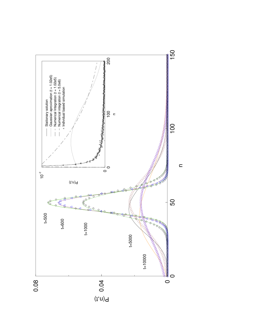
FIG. 7.: Temporal evolution of the relative abundance distribution $P(n,t)$. The parameter values are $N=1000$, $S=50$, $C=0.4$ and $\mu=0.001$. An individual-based simulation, the numerical integration of $P(n,t)$ at two successive times, and the exact stationary solution are also presented (inset).

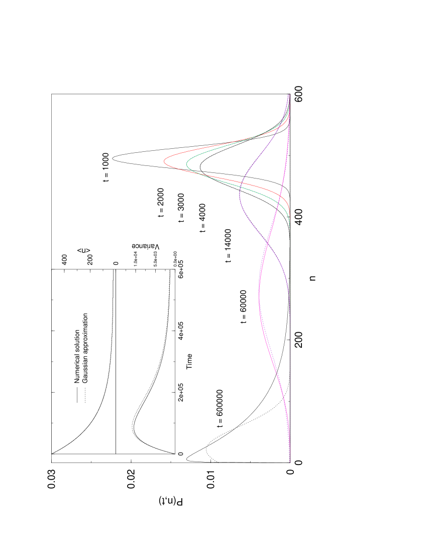
FIG. 8.: Temporal evolution of the relative abundance distribution $P(n,t)$. The parameter values are $N=1000$, $S=50$, $C=0.4$ and $\mu=0.01$. The temporal evolution of the variance and the average abundance computed using (66) and (60) respectively and from the master equation is also shown (inset).

In order to compare the time behavior of the mean field approach introduced in this work through the master equation (4) with the time behavior of the individual based model (IBM) defined by the rules presented in section I, one should carefully define what is meant by time. Individual based simulations are performed by the iteration of an algorithm from the first step up to a given number of updating steps. In section 1, such an updating step has been defined as a time unit. Let us call it the simulation time unit. In [5] a different operational choice was made. Whatever the convention is, a clear distinction must be made between the simulation time and the physical time needed to compare simulation results with either the numerical integration of the master equation (4) or the large-$N$ solution derived in this section. The question then arises: how is physical time to be tracked in any stochastic realization of the IBM? To analyze this point we will follow an argument given by Renshaw [23]. At any time $t$, the probability of an event occurring in the system can be estimated. Such a probability depends on the system configuration, i.e, the abundance of all present species, and on the relative immigration rate $\mu$ in relation to the internal dynamics rate $1-\mu$. Both rates have dimensions of $T^{-1}$. Obviously, it depends also on the other parameters of the model ($N$, $S$ and $C$). Although the method described in Ref [23] estimates every transition probability rate for all possible events in the system, there is no need to estimate the probability of this rather high number of possible events. There are only two relevant temporal processes: immigration and internal dynamics. So, it is enough to consider these two different possibilities:

1. An immigration event $I$ occurs if any species from the pool happens to enter the system. The probability of a pool species entering the system in any small $dt$ is:

   $$Pr\{I\}=r_{I}(t)\,dt\,,$$

   where the immigration rate is

   $$r_{I}=\frac{\mu}{S}\sum_{i=1}^{S}\left(1-\frac{n_{i}(t)}{N}\right)\,.$$

2. An internal dynamics event $D$ occurs when the interaction between a pair of individuals from two potentially interacting species gives rise to a change in their abundances. The probability of such an event occurring in any small $dt$ can be written as:

   $$Pr\{D\}=r_{D}\,dt\,,$$

   where the internal dynamics rate is

   $$r_{D}=(1-\mu)\,\sum_{i=1}^{S}\sum_{j\in{\cal G}(i)}\frac{n_{i}(t)}{N}\frac{n_{j}(t)}{N}\,,$$

   and where ${\cal G}(i)$ must be understood as the set of species — different from $i$ — that are connected to $i$ through the pre-defined interaction matrix $\bf\Omega$.

Since the two events defined are independent from each other, the probability of occurrence of any one of them in any small $dt$ is:

$$Pr\{I\>\cup\>D\}=(r_{I}+r_{D})\,dt\,.$$

When an event occurs there is a change in the actual configuration of the system either by immigration or by internal dynamics and the rates must be calculated again. So, approximately, on average the number of such effective events in any time interval of length $t$ would be $(r_{I}+r_{D})\,t$, and would be distributed as a Poisson random variable with that mean. The important point is that now the probability of having no events in any time interval of length $t$, i.e, for any time between $0$ and $t$, can be written as:

$$Pr\{0\}=e^{-(r_{I}+r_{D})\,t}\,.$$ (68)

According to (68), the probability of having at least one event is $1-e^{-(r_{I}+r_{D})\,t}$ — the cumulative probability distribution for an exponentially distributed random variable. Therefore, the time to the next event is an exponentially distributed random variable with expectation $1/(r_{I}+r_{D})$. Then, we should sample that distribution in order to predict when the next effective event will take place. Accumulating these inter-event times during simulations we are able to track the physical time, which have the same units as $[r_{I}+r_{D}]^{-1}$, so the same time units which arise in the master equation (4).

In figure 9, the time evolution of the number of species in the system is shown. Different stochastic realizations of the IBM are presented. The numerical integration of the master equation allows the estimation of the expected number of species at any time in the system $<S>$ through (35). The average behavior of the different stochastic simulations is well captured by the prediction given by (35) where $P(0,t)$ is computed at each numerical integration time step.

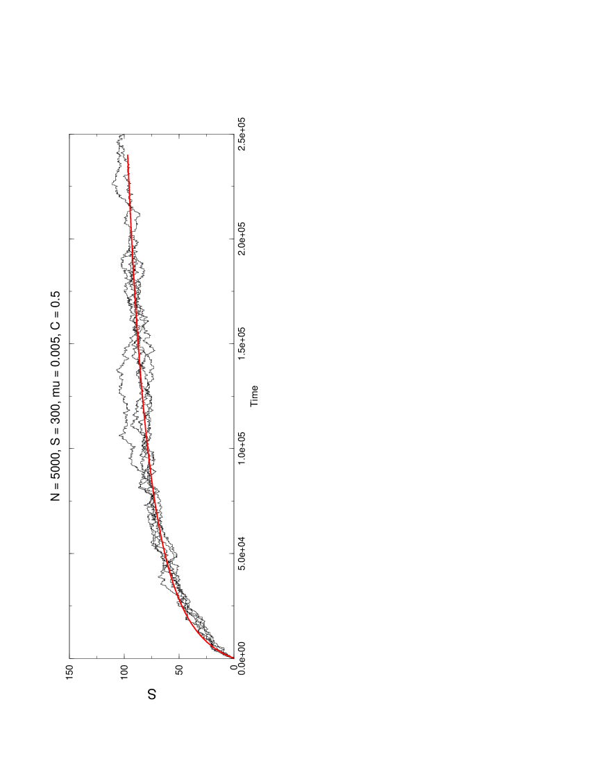
FIG. 9.: Time evolution of the number of species in the system. The individual-based simulations match the expected value from the master equation. The system starts with no species. During the stochastic assembly process the number of species fluctuates, but the average behaviour is captured by the mean field approach represented by the master equation (4).

In Fig 10 the probability of having a species represented by $n$ individuals at particular early times, $P(n,t)$, has been plotted. It has been computed by performing a numerical integration of the master equation (4) (dotted line) and by means an ensemble average for the individual-based model after 5000 simulation time steps. Two extremely different initial conditions have been used. In the first one, there are no species in the system at time $0$. Species enter the system and either establish themselves in it or not, performing what could be called a stochastic community assembly. In the second initial state, all species are represented in approximately equal numbers. Obviously, the one-humped distributions are obtained when the initial condition is a random mixture of species, which is represented by $P(n,0)=1$ if $n=N/S$ and $P(n,t)=0$ if $n\neq N/S$ in the master equation approach. The purely decreasing distributions are obtained when the initial state is a completely empty system. The agreement between the mean field approach represented by the master equation and the simulations is seen to be reasonable.

FIG. 10.: Individual-based model and the temporal evolution of $P(n,t)$. Comparison between the mean field approach (dotted line) and a 2000 ensemble average after 5000 simulation time steps for random mixture and empty system initial conditions. In the first case, two different numerical integrations have been performed for $t=9946$ and $t=10400$. In the second case, just one numerical integration has been performed until $t=6725$. The reason for these different times is that 5000 simulation updating steps can represent more or less physical time depending on the initial configuration of the system.

As it has been shown in Figs 7 and 8, eventually, the probability distribution deviates from a Gaussian. While it is true that one could in principle calculate these non-Gaussian effects using van Kampen’s approach (by taking higher order terms in $N^{-1/2}$ into account), the method gets increasingly cumbersome. Therefore, in the next section, we adopt a totally different approach to the calculation of time-dependence, which is able to give information about $P(n,t)$ at late times.

V generating function

The technique we will use to probe the time-dependence of $P(n,t)$ in this section is based on the solution of the differential equation satisfied by the generating function

$$F(z,t)=\sum^{N}_{n=0}\,P(n,t)z^{n}$$ (69)

for our model in the mean-field approximation. Starting from (4) the derivation of this equation proceeds along standard lines [10, 11] to yield

$$\frac{\partial F}{\partial s}=-z(1-z)^{2}\frac{\partial^{2}F}{\partial z^{2}}+(1-z)(\alpha+\beta z)\frac{\partial F}{\partial z}-\gamma(1-z)F$$ (70)

where we have introduced a new time

$$s=\zeta t\,,\ \ \ {\rm where}\ \ \zeta=\frac{C^{*}}{N(N-1)}\,,$$ (71)

and where the constants $\alpha$, $\beta$ and $\gamma$ are defined by

$$\alpha=\nu^{*}-1=\lambda^{*}(S-1)+N-1\,,$$

$$\beta=\lambda^{*}+1-N\ \ \ {\rm and}\ \ \ \gamma=N\lambda^{*}\,.$$ (72)

The conditions on $F$ are

$$F(1,t)=1\ \ \ {\rm and}\ \ \ F(z,0)=z^{m}\,,$$ (73)

and follow from the normalization condition $\sum_{n}P(n,t)=1$ and the initial condition $P(n,0)=\delta_{n,m}$ respectively.

The partial differential equation (70) is separable: if we write $F(z,s)={\cal S}(s)\Phi(z)$, then ${\cal S}(s)=e^{-\lambda s}$, where $\lambda$ is a constant. The equation for $\Phi$ is then

$$z(1-z)^{2}\frac{d^{2}\Phi}{dz^{2}}-(1-z)(\alpha+\beta z)\frac{d\Phi}{dz}+\gamma(1-z)\Phi=\lambda\Phi\,.$$ (74)

This can be brought into a more standard form by the change of variables

$$\Phi=(1-z)^{N}\phi\ \ \ {\rm and}\ \ u=\frac{1}{1-z}\,.$$ (75)

The new form of the equation is

$$u(1-u)\frac{d^{2}\phi}{du^{2}}+\left[c-(a+b+1)u\right]\frac{d\phi}{du}-ab\phi=0\,,$$ (76)

where

$$a+b=1-\lambda^{*}-N-\nu^{*}\,,$$

$$ab=N\left(\lambda^{*}+\nu^{*}-1\right)-\lambda\ \ \ {\rm and}\ \ \ c=1-\lambda^{*}-N\,.$$ (77)

The reason for making the transformation (75) is that (76) is the standard form for the hypergeometric equation [12], which has the two independent solutions:

$$\phi^{(1)}_{\lambda} = u^{-a}\,F(a,a-c+1,a-b+1;u^{-1})\ \ \ {\rm and}$$ (78)

$$\phi^{(2)}_{\lambda} = u^{-b}\,F(b,b-c+1,b-a+1;u^{-1})\,.$$ (79)

Now $u^{-1}=1-z$ and so in terms of the original variables

$$\Phi^{(1)}_{\lambda} = (1-z)^{N+a}\,F(a,a-c+1,a-b+1;1-z)\ \ \ {\rm and}$$ (80)

$$\Phi^{(2)}_{\lambda} = (1-z)^{N+b}\,F(b,b-c+1,b-a+1;1-z)\,.$$ (81)

The general solution to (70) is then

$$F(z,t)=\sum_{\lambda}\left\{v_{\lambda}\,\Phi^{(1)}_{\lambda}+w_{\lambda}\,\Phi^{(2)}_{\lambda}\right\}\,e^{-\lambda\zeta t}\,,$$ (82)

where $\{v_{\lambda}\}$ and $\{w_{\lambda}\}$ are sets of arbitrary constants.

To determine the arbitrary constants in (82), the conditions (73) have to be implemented. The details are given in Appendix B, where it is shown that the required solution is

$$F(z,t)=\sum_{k=0}^{N}\,w_{k}\,(1-z)^{k}\,F(k-N,k+\lambda^{*},2k+\lambda^{*}S;1-z)\,e^{-k(k+\lambda^{*}S-1)\zeta t}\,,$$ (83)

where the constants $\{w_{k}\}$ are determined by

$$\sum^{n}_{k=0}\,w_{k}\,(-1)^{n-k}\,{N-k\choose n-k}\,\frac{\Gamma(n+\lambda^{*})\,\Gamma(2k+\lambda^{*}S)}{\Gamma(k+\lambda^{*})\,\Gamma(n+k+\lambda^{*}S)}=\left\{\begin{array}[]{ll}(-1)^{n}\,{m\choose n},&\mbox{\ if $n\leq m$}\\ \ \ \ \ \ \ 0\ \ \ \ \ \ ,&\mbox{\ if $n>m$\, .}\end{array}\right.$$ (84)

This equation holds for all allowed values of $n$ ($n=0,1,\ldots,N$). We therefore have $(N+1)$ linear conditions for the $(N+1)$ constants $w_{k}$ ($k=0,1,\ldots,N$), and so can determine them uniquely. Thus, (83) together with (84) provide a complete solution to the partial differential equation (70).

Although the solution is not in closed form, it is possible to obtain the $w_{k}$ for small values of $k$ rather easily. For $n=0$, (84) involves only $w_{0}$, for $n=1$ only $w_{0}$ and $w_{1}$, and so on. The expressions for the first three constants are

$$w_{0} = 1\,,\ \ \ w_{1}=\frac{N}{S}-m\,,$$ (85)

$$w_{2} = \frac{(N-1)(1+\lambda^{*})}{(2+\lambda^{*}S)}\,\left[\frac{N}{S}-m\right]\ -\ \frac{N(N-1)}{2S}\,\frac{(1+\lambda^{*})}{(1+\lambda^{*}S)}\ +\ \frac{m(m-1)}{2}\,,$$ (86)

the result for $w_{0}$ confirming what we already knew. These results are very useful because, as is clear from (83), the large-time behavior of the system is governed by small values of $k$. In this case, as we will now show, an explicit form for $P(n,t)$ can be found.

To find $P(n,t)$ we have the identify the coefficient of $z^{n}$ in (83). In Appendix B it is shown that this leads to

$$P(n,t)=\sum^{N}_{k=0}\,w_{k}\,\chi(n,k)\,e^{-k(k+\lambda^{*}S-1)\zeta t}\,,$$ (87)

where

$$\chi(n,k) = \sum^{r={\rm min}\{N-k,n\}}_{r={\rm max}\{n-k,0\}}\,(-1)^{n-r}\,{k\choose n-r}\,{N-k\choose r}$$ (88)

$$\times {\Gamma(r+k+\lambda^{*})\over\Gamma(k+\lambda^{*})}{\Gamma(\nu^{*}-r)\over\Gamma(k+\nu^{*}-N)}{\Gamma(2k+\lambda^{*}+\nu^{*}-N)\over\Gamma(k+\lambda^{*}+\nu^{*})}\,.$$ (90)

This result appears to be rather complicated, but fortunately it simplifies in many cases of interest. For instance, suppose we wish to find $P(0,t)$: the time-evolution of the probability that there are no individuals of the species present in the system. Since $\chi(0,k)$ has only one term in the sum ($r=0$),

$$P(0,t) = \Gamma(\nu^{*})\,\sum^{N}_{k=0}\,w_{k}\frac{\Gamma(2k+\nu^{*}+\lambda^{*}-N)}{\Gamma(k+\nu^{*}-N)\,\Gamma(k+\nu^{*}+\lambda^{*})}\,e^{-k(k+\lambda^{*}S-1)\zeta t}$$ (91)

$$= P_{s}(0)\left\{1+w_{1}\frac{S(\lambda^{*}S+1)}{(S-1)(\lambda^{*}S+N)}\,e^{-\lambda^{*}S\zeta t}\right.$$ (93)

$$+ \left.w_{2}\frac{S(\lambda^{*}S+1)(\lambda^{*}S+2)(\lambda^{*}S+3)}{(S-1)(\lambda^{*}(S-1)+1)(\lambda^{*}S+N)(\lambda^{*}S+N+1)}\,e^{-2(\lambda^{*}S+1)\zeta t}+\ldots\right\}\,,$$ (95)

which describes the approach to the stationary state at large times. In Fig 11 the temporal evolution of the expected number of species, estimated as $S(t)=S(1-P(0,t))$ is shown. The temporal solution provided by this method is exact as long as the total number of coefficients can be computed without numerical error. In Fig 11 a truncated, approximated solution is compared with the straightforward numerical integration of the master equation. Complete agreement is observed at large times.

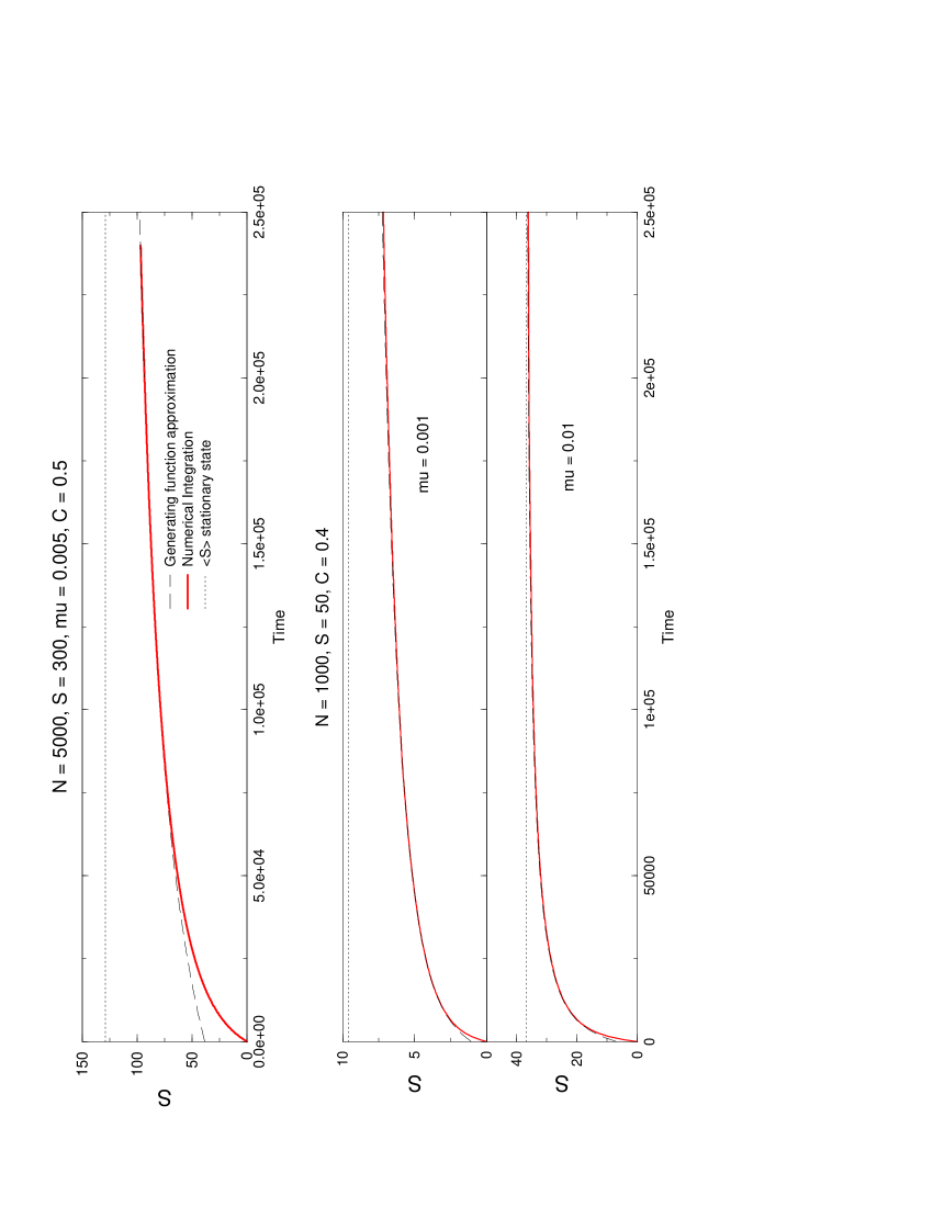
FIG. 11.: Temporal evolution of the expected value for the number of species in the system. A truncated solution provided by (95) is shown (dashed-lines). Only the first 20 $w_{k}$ coefficients have been computed. The agreement with the numerical integration of the master equation (bold lines) gets better and better the larger time is. For $N=1000$, $S=50$, and $C=0.4$ such an agreement is quite good even for early times.

If $n\neq 0$, the large time behavior of $P(n,t)$ still has a relatively simple form:

$$P(n,t) = P_{s}(n)+w_{1}\,\chi(n,1)\,e^{-\lambda^{*}S\zeta t}$$ (96)

$$+ w_{2}\,\chi(n,2)\,e^{-2(\lambda^{*}S+1)\zeta t}+\ldots\,,$$ (97)

where $\chi(n,1)$ has only two terms, $r=n-1$ and $r=n$ (only one if $n=0$ or $n=N$) and $\chi(n,2)$ has only three terms, $r=n-2,n-1$ and $n$ (fewer if $n=0,1,N-1$ or $N$).

In Fig 12, the computation of $P(n,t)$ for $n=1,2,3,4$ is shown. The solution is approximate because again just the first 20 $w_{k}$ have been considered, although (87) would be an exact solution as long as all of the terms from $k=0$ to $k=N$ could be summed without numerical error. For practical reasons this is obviously not possible. In particular, at early times, the truncation of (87) introduces errors in $P(n,t)$. The same is true when $n$ is too large, because the sums in (84) and (90) are too long to be computed without errors and some numerical instabilities arise.

FIG. 12.: Temporal evolution of probability of having any species represented by 1, 2, 3, and 4 individuals computed directly from (87) in dotted lines, where again a truncated solution is used (only the first 20 $w_{k}$ are considered), compared with the numerical integration of the master equation (bold lines). The initial condition is $P(n,0)=\delta_{m,n}$ where $m=500$ in the upper plot and $m=0$ in the lower one.

VI Conclusions

In this paper we have analysed a model which has a structure which is rich enough to show many of the underlying patterns seen in real ecosystems, but is still sufficiently simple for a variant of the mean field approximation to be applied to obtain analytical results. The most straightforward question that can be asked concerns the nature of the stationary state. Within the mean field approximation an exact form for this stationary distribution may be derived. We found that this exact result reduced to the logseries distribution in the regime of low immigration and to the lognormal distribution in the regime of moderate to high immigration. These two distributions have been discussed by ecologists for decades as possible forms for the species abundance distributions. Our approach gives a clear interpretation to the parameters on which they depend. This fact has practical consequences for conservation biology in order to determine the potential richness ($S$), the global size ($N$) and the degree of isolation (${\mu}$) of a community. We have therefore shown how logseries and lognormal distributions can arise as two different limits of a single distribution, a distribution which is, moreover, the stationary distribution of a well-motivated ecological model. We also found evidence for the hyperbolic relation between the connectivity and the average number of species — the so-called $C^{*}-S$ relation. While we were able to derive this result in the low immigration regime, there was a small systematic derivation from the mean-field result and the simulation curves.

While the stationary distribution is of considerable interest, the strength of the approach that we have adopted here is that predictions of the time evolution of the system are also possible. An approximation based on the number of individuals in the system being large led to the picture of $P(n,t)$ as an approximately Gaussian distribution broadening and moving with time. This behavior may persist for quite a long time, especially when the immigration rate is high, but eventually the Gaussian form is lost at large times. To explore the approach to the stationary distribution a complimentary formalism was required. Such a method was discussed in section V where a formal general solution for the temporal evolution of the probability of having any species represented by $n$ individuals is given. This solution $P(n,t)$ is given as a series expansion around the stationary state. In particular, such a solution allows one to predict quite well how the number of species in the system increases with time during the stochastic assembly process.

In summary, we believe that this simple model has illuminated the general mechanisms at work in ecosystems and has allowed us to understand the broad features of some of the universal phenomena seen in these systems. We hope that the results presented here will motivate further work both in the increasingly sophisticated stochastic modelling of ecosystems and in the interpretation of ecological data within a theoretical framework.

A

In this appendix we will give details of the derivations of the simpler forms of the stationary distribution discussed in section III.

In our analysis, we will frequently make use of the asymptotic form for $\Gamma(z+a)/\Gamma(z)$ when $z\gtrsim 1$ and $z\gg a$. Using Stirling’s approximation for $z\gtrsim 1$ one has that

$$\frac{\Gamma(z+a)}{\Gamma(z)}=z^{a}\left(1+\frac{a}{z}\right)^{(z+a-1/2)}\,\exp{(-a)}$$

$$\times\left[1+P_{1}(z)\left(\frac{a}{z}\right)+P_{2}(z)\left(\frac{a}{z}\right)^{2}+...\ \right]\,,$$

where the $P_{i}(z)$ are power series in $1/z$. Therefore, if in addition we impose the condition $a\ll z$, then to a very good approximation

$$\frac{\Gamma(z+a)}{\Gamma(z)}\approx(1+\epsilon)^{z(1+\epsilon)}\,z^{a}\,e^{-a}\ \ ;\ z\gtrsim 1\ ;\ \epsilon=\frac{a}{z}\ll 1\,.$$ (A1)

Note that $a$ need not be small, it simply has to be much less than $z$.

Applying (A1) to ${\cal F}_{3}(n,N)$ one finds ($N\gg 1\Rightarrow\nu^{*}\gg 1$)

$${\cal F}_{3}(n,N) = \left[\frac{\Gamma(N+1-n)}{\Gamma(N+1)}\right]^{-1}\left[\frac{\Gamma(\nu^{*}-n)}{\Gamma(\nu^{*})}\right]$$ (A2)

$$\approx \left(\frac{N+1}{\nu^{*}}\right)^{n}\left\{\left(1-\frac{n}{N+1}\right)^{-(N+1-n)}\left(1-\frac{n}{\nu^{*}}\right)^{(\nu^{*}-n)}\right\}\,.$$ (A4)

The term in curly brackets is equal to one, plus corrections which are negligible if $n_{\rm max}^{2}\lambda^{*}S/N^{2}\ll 1$ and $\lambda^{*}S\ll N$. Therefore, under these conditions

$${\cal F}_{3}(n,N)\approx\left(\frac{N}{\nu^{*}}\right)^{n} \approx \exp{-n\ln\left(1+\frac{\lambda^{*}S}{N}\right)}$$ (A5)

$$\approx \exp{\left(-n\lambda^{*}S/N\right)}\,,$$ (A6)

using $S\gg 1$ and $\lambda^{*}S\ll N$ again.

To find a simpler form for ${\cal F}_{1}(n)$, we again apply (A1), but with the more stringent condition $a\ll 1$. It then becomes $\Gamma(z+a)/\Gamma(z)\approx z^{a}$, and so for $\lambda^{*}\ll 1$ and $n\gtrsim 1$

$${\cal F}_{1}(n)=\frac{1}{n\,\Gamma(\lambda^{*})}\,\frac{\Gamma(n+\lambda^{*})}{\Gamma(n)}\approx\frac{\lambda^{*}n^{\lambda^{*}}}{n}=\frac{\lambda^{*}}{n}\exp{\lambda^{*}\ln n}\,.$$ (A7)

If we now ask that $\lambda^{*}\ln n_{\rm max}\ll 1$, we have that

$${\cal F}_{1}(n)\approx\frac{\lambda^{*}}{n}\ \ ;\ n\gtrsim 1\ ;\ \lambda^{*}\ll\frac{1}{\ln n_{\rm max}}\,.$$ (A8)

To estimate $P_{s}(0)$ we apply (A1) directly to ${\cal F}_{2}(N)$ in (27). Assuming $\lambda^{*}S\gtrsim 1$

$${\cal F}_{2}(N) = \left[\frac{\Gamma(\nu^{*}+\lambda^{*})}{\Gamma(\nu^{*})}\right]^{-1}\left[\frac{\Gamma([\nu^{*}-N]+\lambda^{*})}{\Gamma(\nu^{*}-N)}\right]$$ (A9)

$$\approx \left(\frac{\nu^{*}-N}{\nu^{*}}\right)^{\lambda^{*}}\left\{\left(1+\frac{\lambda^{*}}{\nu^{*}}\right)^{-(\nu^{*}+\lambda^{*})}\left(1+\frac{\lambda^{*}}{\nu^{*}-N}\right)^{(\nu^{*}-N+\lambda^{*})}\right\}\,.$$ (A11)

Under the very reasonable assumptions $(\lambda^{*})^{2}\ll N$ and $\lambda^{*}\ll S$, the curly brackets approximate very well to unity, and so if in addition $\lambda^{*}S\ll N$,

$${\cal F}_{2}(N)\approx\left(\frac{\lambda^{*}S}{N+\lambda^{*}S}\right)^{\lambda^{*}}\approx\left(\frac{\lambda^{*}S}{N}\right)^{\lambda^{*}}\approx\left(\mu^{*}S\right)^{\lambda^{*}}\,.$$ (A12)

This result may be used to find a useful expression for the average number of species, $\langle S\rangle$ defined by (35). Since $P_{s}(0)\approx\exp{\lambda^{*}\ln(\lambda^{*}S/N)}$, it follows that

$$\langle S\rangle\approx\left(1-\exp{\lambda^{*}\ln(\lambda^{*}S/N)}\right)S\approx S\lambda^{*}\ln\left(\frac{N}{S\lambda^{*}}\right)\,,$$ (A13)

if $\lambda^{*}\ln(N/S\lambda^{*})\ll 1$. We now write

$$\ln\left(N/S\lambda^{*}\right) = \ln\left([1-\mu]C^{*}/\mu\right)$$ (A14)

$$= \epsilon^{-1}+\ln C^{*}\,,\ \ \ \ {\rm where\ }\epsilon^{-1}\equiv\ln\left(\frac{1-\mu}{\mu}\right)$$ (A15)

$$\approx \epsilon^{-1}\exp{\epsilon\ln C^{*}}\,,$$ (A16)

if $\epsilon|\ln C^{*}|\ll 1$.

Now suppose that we assume that $\lambda^{*}\ll\epsilon$ and $\epsilon|\ln C^{*}|\ll 1$. It follows that $\lambda^{*}\epsilon^{-1}[1+\epsilon|\ln C^{*}|]\ll 1$ and therefore that $\lambda^{*}\ln(N/S\lambda^{*})\ll 1$. Thus this latter condition may be replaced by $\lambda^{*}\ll\epsilon$ and $\epsilon|\ln C^{*}|\ll 1$. The immigration rate $\mu$ is typically much less than one, so $\epsilon^{-1}\approx|\ln\mu|$. Therefore the last condition becomes $|\ln C^{*}|\ll|\ln\mu|$. Putting all of this together, we find that

$$\langle S\rangle\approx\frac{\lambda^{*}S}{\epsilon}\left(C^{*}\right)^{\epsilon}=\frac{N\mu}{(1-\mu)\epsilon}\left(C^{*}\right)^{-1+\epsilon}\,,$$ (A17)

if $\lambda^{*}S\gtrsim 1$ (since we have used (A12)), $\lambda^{*}\ll\epsilon$ and $|\ln C^{*}|\ll|\ln\mu|$.

B

In this appendix we give details of the calculations presented in section V. We begin by showing that is we apply the conditions (73) to the general solution (82) of the partial differential equation (70), we obtain (83) with the constants $\{w_{k}\}$ being determined by (84).

First, let us apply the condition $F(1,t)=1$. Now $\Phi^{(1)}_{\lambda}\approx(1-z)^{N+a}$ and $\Phi^{(2)}_{\lambda}\approx(1-z)^{N+b}$ as $z\rightarrow 1$. So define $\tilde{a}=N+a$ and $\tilde{b}=N+b$. Then from (77),

$$\tilde{a} = \frac{\left[1-\lambda^{*}S\right]-\sqrt{\left[1-\lambda^{*}S\right]^{2}+4\lambda}}{2}$$ (B1)

$$\tilde{b} = \frac{\left[1-\lambda^{*}S\right]+\sqrt{\left[1-\lambda^{*}S\right]^{2}+4\lambda}}{2}\,,$$ (B2)

with $\tilde{a}\tilde{b}=-\lambda$. Since the constants $a$ and $b$ appear in the differential equation (76) symmetrically, we have made a choice as to which has the positive and which has the negative square root. From the general theory of the master equation [10], the eigenvalues $\lambda$ are real and non-negative, and so $\tilde{a}$ and $\tilde{b}$ are real. Moreover, if $\lambda\neq 0$, they are of different signs, since their product is negative. With the choice (B2), $\tilde{a}<0$ and $\tilde{b}>0$. From these results we deduce that $\Phi^{(1)}_{\lambda}$ diverges and $\Phi^{(2)}_{\lambda}\rightarrow 0$ as $z\rightarrow 1$. We must therefore take $v_{\lambda}=0$ for all $\lambda>0$. When $\lambda=0$, $\tilde{b}=1-\lambda^{*}S$, which may be negative, and so we also take $w_{0}=0$. Finally, $\tilde{a}=0$ when $\lambda=0$ and so this term is the only one which is not zero or does not diverge as $z\rightarrow 1$. Since the $\lambda=0$ solution is the stationary solution, the condition $F(1,t)=1$ is automatically satisfied as long as the stationary solution is normalized. Therefore, the application of this condition has reduced (82) to

$$F(z,t)=F_{s}(z)+\sum_{\lambda>0}\,w_{\lambda}\,(1-z)^{N+b}\,F(b,b-c+1,b-a+1;1-z)\,e^{-\lambda\zeta t}\,,$$ (B3)

where $F_{s}(z)=\sum_{n}P_{s}(n)z^{n}$.

Before proceeding any further, we need to investigate the sum over $\lambda$ more carefully. We know that this sum should be over a set of discrete integers: $F(z,t)=\sum_{n}P(n,t)z^{n}\,,\ n\in\{0,1,\ldots,N\}$. An analysis of the structure of the hypergeometric function in (B3) for large $z$ shows that this will only be so if $b$ is equal to an integer which is zero or negative: $b=-l$. We can understand this condition by recalling [12] that the function $F(a^{\prime},b^{\prime},c^{\prime};x)$ is a polynomial of degree $l$ (where $l$ is a non-negative integer) in $x$ if $a^{\prime}=-l$. Therefore, if $b=-l$, then $F$ in (B3) must be a polynomial of degree $l$ in $(1-z)$, i.e. $(1-z)^{N+b}F$ must be a polynomial of degree $N+b+l=N$ in $(1-z)$, as required.

From (B2), $\tilde{a}+\tilde{b}=\left[1-\lambda^{*}S\right]$, so if $\tilde{b}=N+b=(N-l)$, then $\tilde{a}=l-N+\left[1-\lambda^{*}S\right]$. Similarly, $\tilde{b}-\tilde{a}=2N-2l-\left[1-\lambda^{*}S\right]=\sqrt{[1-\lambda^{*}S]^{2}+4\lambda}$. A short calculation then gives $\lambda=(N-l)(\omega-l)$, where $\omega=N+\lambda^{*}S-1$. Since we require $\lambda>0$ in the sum in (B3), then $l=0,1,\ldots,N-1$. So, in summary,

$$\lambda=(N-l)(\omega-l)\ \ \ \ l=0,1,\ldots,N-1$$ ; (B4)

$$a=l-N-\omega\ \ ;\ \ b = -l\ \ ;\ \ c=1-\lambda^{*}-N\,,$$ (B5)

where

$$\omega\equiv N+\lambda^{*}S-1\,.$$ (B6)

Rather than $l$, it is preferable to use $k\equiv N-l$ to label the time-dependent solutions. Then (B3) becomes

$$F(z,t)=F_{s}(z)+\sum_{k=1}^{N}\,w_{k}\,(1-z)^{k}\,F(k-N,k+\lambda^{*},2k+\lambda^{*}S;1-z)\,e^{-k(k+\lambda^{*}S-1)\zeta t}\,,$$ (B7)

where we have written $w_{\lambda(l)}$ as $w_{k}$ for convenience. We note that if there were a $k=0$ term in the sum, it would equal $w_{0}\,F(-N,\lambda^{*},\lambda^{*}S;1-z)$ which in turn equals [12]

$$w_{0}\,\frac{\Gamma(\nu^{*})\Gamma(\nu^{*}+\lambda^{*}-N)}{\Gamma(\nu^{*}-N)\Gamma(\nu^{*}+\lambda^{*})}\,F(-N,\lambda^{*},1-\nu^{*};z)$$

$$=w_{0}\,\sum_{n=0}^{N}\,{N\choose n}{\Gamma(n+\lambda^{*})\over\Gamma(\lambda^{*})}{\Gamma(\nu^{*}-n)\over\Gamma(\nu^{*}-N)}{\Gamma(\lambda^{*}+\nu^{*}-N)\over\Gamma(\lambda^{*}+\nu^{*})}\,z^{n}\,$$ (B8)

which equals $w_{0}\,\sum_{n}P_{s}(n)z^{n}$, using (17). Therefore (B7) may be written in the alternative form

$$F(z,t)=\sum_{k=0}^{N}\,w_{k}\,(1-z)^{k}\,F(k-N,k+\lambda^{*},2k+\lambda^{*}S;1-z)\,e^{-k(k+\lambda^{*}S-1)\zeta t}\,,$$ (B9)

where $w_{0}=1$. It is also possible to write the function $F$ in (B9) as a Jacobi polynomial of order $N-k$ [12].

The final step is to apply the initial condition given in (73) to (B9) in order to determine the sets of constants $\{w_{k}\}$. This leads to

$$z^{m}=\sum_{k=0}^{N}\,w_{k}\,(1-z)^{k}\,F(k-N,k+\lambda^{*},2k+\lambda^{*}S;1-z)\,.$$ (B10)

To solve (B10), let us write the hypergeometric function as

$$F=\sum_{n=0}^{N-k}\,f_{n}(1-z)^{n}\ \ \ {\rm where}\ \ f_{n}=(-1)^{n}\,{N-k\choose n}\,\frac{(k+\lambda^{*})_{n}}{(2k+\lambda^{*}S)_{n}}\,,$$ (B11)

where the symbol $(a)_{n}$ means $\Gamma(a+n)/\Gamma(a)$. Then rearranging the double sum gives

$$z^{m}=\sum^{N}_{n=0}\,(1-z)^{n}\sum^{n}_{k=0}\,w_{k}\,f_{n-k}=\sum^{N}_{n=0}\,c_{n}\,(1-z)^{n}\,,$$ (B12)

where $c_{n}=\sum^{n}_{k=0}\,w_{k}\,f_{n-k}$. However, it is straightforward to determine the $c_{n}$: by expanding $(1-[1-z])^{m}$ in powers of $(1-z)$ we find that $c_{n}$ vanishes for $n>m$ and is proportional to a binomial coefficient for $n\leq m$. Using this result and writing out $f_{n-k}$ fully yields

$$\sum^{n}_{k=0}\,w_{k}\,(-1)^{n-k}\,{N-k\choose n-k}\,\frac{\Gamma(n+\lambda^{*})\,\Gamma(2k+\lambda^{*}S)}{\Gamma(k+\lambda^{*})\,\Gamma(n+k+\lambda^{*}S)}=\left\{\begin{array}[]{ll}(-1)^{n}\,{m\choose n},&\mbox{\ if $n\leq m$}\\ \ \ \ \ \ \ 0\ \ \ \ \ \ ,&\mbox{\ if $n>m$\, .}\end{array}\right.$$ (B13)

We now turn to the problem of finding $P(n,t)$, which involves identifying the the coefficient of $z^{n}$ in (B9). Let us begin by considering $F(k-N,k+\lambda^{*},2k+\lambda^{*}S;1-z)$. By following exactly the same steps that lead to (B8) in the $k=0$ case, but this time for general $k$, we find that this function equals

$$\frac{\Gamma(\nu^{*})\Gamma(2k+\nu^{*}+\lambda^{*}-N)}{\Gamma(k+\nu^{*}-N)\Gamma(k+\nu^{*}+\lambda^{*})}\,F(k-N,k+\lambda^{*},1-\nu^{*};z)$$

$$=\sum_{r=0}^{N-k}\,{N-k\choose r}{\Gamma(r+k+\lambda^{*})\over\Gamma(k+\lambda^{*})}{\Gamma(\nu^{*}-r)\over\Gamma(k+\nu^{*}-N)}{\Gamma(2k+\lambda^{*}+\nu^{*}-N)\over\Gamma(k+\lambda^{*}+\nu^{*})}\,z^{r}\,,$$ (B14)

Therefore, we may write the solution for $F(z,t)$, eqn. (B9), as

$$F(z,t)=\sum^{N}_{k=0}\,w_{k}(1-z)^{k}\,\sum^{N-k}_{r=0}\,\rho_{r}(k)z^{r}e^{-k(k+\lambda^{*}S-1)\zeta t}\,,$$ (B15)

where

$$\rho_{r}(k)={N-k\choose r}{\Gamma(r+k+\lambda^{*})\over\Gamma(k+\lambda^{*})}{\Gamma(\nu^{*}-r)\over\Gamma(k+\nu^{*}-N)}{\Gamma(2k+\lambda^{*}+\nu^{*}-N)\over\Gamma(k+\lambda^{*}+\nu^{*})}\,.$$ (B16)

To identify powers of $z$ in (B15) we break it down further:

$$F(z,t)=\sum^{N}_{k=0}\,w_{k}\,e^{-k(k+\lambda^{*}S-1)\zeta t}\,\sum^{k}_{l=0}\,(-1)^{l}{k\choose l}\,\sum^{N-k}_{r=0}\,\rho_{r}(k)z^{r+l}\,.$$ (B17)

Writing

$$\sum^{k}_{l=0}\,(-1)^{l}{k\choose l}\,\sum^{N-k}_{r=0}\,\rho_{r}(k)z^{r+l}=\sum^{N}_{n=0}\,\chi(n,k)\,z^{n}\,,$$ (B18)

we have from (B17)

$$F(z,t) = \sum^{N}_{k=0}\,w_{k}\,e^{-k(k+\lambda^{*}S-1)\zeta t}\,\sum^{N}_{n=0}\,\chi(n,k)\,z^{n}$$ (B19)

$$= \sum^{N}_{n=0}\,\left\{\sum^{N}_{k=0}\,w_{k}\,\chi(n,k)\,e^{-k(k+\lambda^{*}S-1)\zeta t}\right\}z^{n}$$ (B21)

$$\Rightarrow\ \ \ P(n,t) = \sum^{N}_{k=0}\,w_{k}\,\chi(n,k)\,e^{-k(k+\lambda^{*}S-1)\zeta t}\,.$$ (B23)

So to find $P(n,t)$ we have to determine $\chi(n,k)$, which is the coefficient of $z^{n}$ in (B18). If we denote $(-1)^{l}{k\choose l}$ by $a_{l}$ and $\rho_{r}(k)$ by $b_{r}$, this is like asking: what is the coefficient of $z^{n}$ in

$$\left[a_{0}+a_{1}z+\ldots+a_{k}z^{k}\right]\left[b_{0}+b_{1}z+\ldots+b_{N-k}z^{N-k}\right]\,?$$

The answer is:

$$\sum^{r={\rm min}\{N-k,n\}}_{r={\rm max}\{n-k,0\}}\,a_{n-r}b_{r}\,.$$

Going back to the variables relevant to the problem under consideration,

$$\chi(n,k)=\sum^{r={\rm min}\{N-k,n\}}_{r={\rm max}\{n-k,0\}}\,(-1)^{n-r}\,{k\choose n-r}\,\rho_{r}(k)\,.$$ (B24)

The complicated limits on the sum can be relaxed with a suitable interpretation of the binomial coefficient ${M\choose L}$. For instance,

$$(-1)^{n-r}\,{k\choose n-r}=\frac{\Gamma(-k+[n-r])}{(n-r)\,!\,\Gamma(-k)}\,.$$

If $(n-r)\leq k$, both the numerator and the denominator on the right-hand-side diverge in such a way that the ratio is finite and non-zero and is commonly written as the left-hand-side. If $(n-r)>k$, then only the denominator diverges and the right-hand-side is zero. With this understanding, the lower condition on the sum in (B24) can simply be replaced by $r=0$, since there is no contribution if $(n-r)>k$, that is, if $r<n-k$. A similar interpretation of the binomial coefficient in $\rho_{r}(k)$ can be used to remove the upper condition on the sum. The result (B24), together with the definition of $\rho_{r}(k)$, determine the $P(n,t)$ given by (B23).

REFERENCES

- [1] E. C. Pielou, Mathematical ecology (Wiley, New York, 1977). Second edition. Section IV.
- [2] F. W. Preston, Ecology 43, 185; 410 (1962). Some recent extensive field data analysis from ecosystems has shown that these communities follow a very well defined power law in species abundances: with spanning three to four decades (S. Pueyo [17]).
- [3] R. J. Putman, Community Ecology (Chapman and Hall, London, 1994). Chapter 3; S. L. Pimm, J. H. Lawton and J. E. Cohen, Nature, 350, 699 (1991); K. Havens, Science 257, 1107 (1992), 260, 243 (1993); N. D. Martinez, Science 260, 242 (1993).
- [4] T. H. Keitt, and P. A. Marquet, J. Theor. Biol. 182, 161 (1996); T. H. Keitt and H. E. Stanley, Nature 393, 257 (1998).
- [5] R. V. Solé, D. Alonso and A. J. McKane, Physica A (in press).
- [6] E. P. Odum, Fundamentals of Ecology (Saunders, London, 1971). Third edition.
- [7] R. M. May, Nature 238, 413 (1972); T. Hogg, B. Huberman and J. M. McGlade, Proc. R. Soc. London B237, 43 (1989).
- [8] S. L. Pimm, Food webs (Chapman and Hall, London, 1982); D. O. Logofet, Matrices and graphs: stability problems in mathematical ecology (CRC Press, London, 1993); K. McCann and A. Hastings, Proc. Roy. Soc. Lond. B 264, 1249 (1997); A. R. Solow, C. Costello and A. R. Beet, The American Naturalist 154, 587 (1999).
- [9] S. Jain and S. Krishna, Phys. Rev. Lett. 81, 5684 (1998).
- [10] N. G. Van Kampen, Stochastic Processes in Physics and Chemistry (Elsevier, Amsterdam, 1981).
- [11] C. W. Gardiner, Handbook of Stochastic Methods (Springer, Berlin. 1985). Second edition.
- [12] M. Abramovitz and A. Stegun (eds), Handbook of Mathematical Functions (Dover, New York, 1965).
- [13] R. H. MacArthur and E. O. Wilson The Theory of Island Biogeography, Princeton University Press, Princeton (1967).
- [14] R. M. May, Ecology and Evolution of Communities, M. L. Cody and J. M. Diamond (eds) pp 81-120 (1975).
- [15] R. A. Fisher, A. S. Corbet, C. W. Williams, Journal of Animal Ecology, 12, 42 (1943).
- [16] S. Engen and R. Lande, J. Theor. Biol., 178, 325. (1996).
- [17] S. Pueyo, Ecological Monographs, submitted.
- [18] F. W. Preston, Ecology, 29, 254 (1948).
- [19] F. W. Preston, Ecology, 43, 185, 410 (1962).
- [20] W. H. Press, S. A. Teukolsky, W. T. Vettering and B. P. Flannery, Numerical Recipes. The Art of Scientific Computing (Cambridge University Press, Cambridge, 1988). First edition.
- [21] P. J. DeVries, D. Murray, and R. Lande, Biological Journal of the Linnean Society, 62, 343 (1997)
- [22] R. Margalef, Our Biosphere, (Ecology Institute, Oldenforf/Luhe, Germany, 1997). Pp 91-95.
- [23] E. Renshaw, Modelling Biological Populations in Space and Time (Cambridge University Press, Cambridge, 1991).