TPR-00-08

BIFURCATION CASCADES AND SELF-SIMILARITY OF

PERIODIC ORBITS WITH ANALYTICAL SCALING CONSTANTS

IN HENON-HEILES TYPE POTENTIALS

Matthias Brack

Institute for Theoretical Physics, University of Regensburg

D-93040 Regensburg, Germany

Abstract

We investigate the isochronous bifurcations of the straight-line librating orbit in the Hénon-Heiles and related potentials. With increasing scaled energy $e$, they form a cascade of pitchfork bifurcations that cumulate at the critical saddle-point energy $e=1$. The stable and unstable orbits created at these bifurcations appear in two sequences whose self-similar properties possess an analytical scaling behavior. Different from the standard Feigenbaum scenario in area preserving two-dimensional maps, here the scaling constants $\alpha$ and $\beta$ corresponding to the two spatial directions are identical and equal to the root of the scaling constant $\delta$ that describes the geometric progression of bifurcation energies $e_{n}$ in the limit $n\rightarrow\infty$. The value of $\delta$ is given analytically in terms of the potential parameters.

1. Introduction

The present study arose in the context of applying Martin Gutzwiller’s semiclassical trace formula [2, 3], and some of its extensions, to various model Hamiltonians and interacting fermion systems in the mean-field approximation, with the aim of describing prominent quantum shell effects semiclassically in terms of the leading classical periodic orbits with shortest periods. This approach was promoted by Strutinsky et al. [4], who estimated the nuclear ground-state deformations from the shortest periodic orbits in an ellipsoidal billiard. Applications which involved the author were beats in the level density of the Hénon-Heiles and related potentials [5, 6], conductance oscillations in mesoscopic semiconductor structures [7, 8], and the onset of mass asymmetry in nuclear fission [9]. We refer to the literature just quoted and to a recent monograph [10] for a detailed discussion of the extensions of Gutzwiller’s theory that are adequate for treating the degenerate orbit families occurring in systems with continuous symmetries. Uniform approximations that become necessary in connection with symmetry breaking and bifurcations will be referred to in the next section. The accumulated experience from these investigations is an astonishing performance of the periodic orbit theory in reproducing quantum-mechanical gross-shell structure, using just a few short periodic orbits in the appropriate semiclassical trace formulae.

In the present paper, we will stay on a purely classical level and investigate the onset of chaos in the Hénon-Heiles and related potentials through bifurcation cascades, the accompanying self-similarity of periodic orbits, and their analytical scaling behavior.

2. The Hénon-Heiles potential

We investigate here the role of the straight-line librating orbit A in the Hénon-Heiles (HH) Hamiltonian [11]:

$$H=\frac{1}{2}\,({\dot{x}}^{2}+{\dot{y}}^{2})+\frac{1}{2}\,(x^{2}+y^{2})+\varepsilon\,(x^{2}y-\frac{1}{3}\,y^{3})\,.$$ (1)

Introducing the scaled variables $u=\varepsilon x$ and $v=\varepsilon y$, the scaled total energy $e$, in units of the saddle-point energy $E^{*}=1/6\varepsilon^{2}$, becomes

$$e=E/E^{*}=6\left[\frac{1}{2}({\dot{u}}^{2}+{\dot{v}}^{2})+V(u,v)\right]=\,3\,({\dot{u}}^{2}+{\dot{v}}^{2})+3\,(u^{2}+v^{2})+6\,v\,u^{2}-2\,v^{3}.$$ (2)

The Newton equations of motion in $u,v$ are

$$\ddot{u} = -u\,(1+2v)\,,$$

$$\ddot{v} = -v+v^{2}-u^{2}.$$ (3)

These equations, and therefore the classical dynamics of the HH potential, depend only on the scaled energy $e$ as a single parameter. For our numerical investigations below, we have solved Eqs. (3) numerically and determined the periodic orbits by a Newton-Raphson iteration using their stability matrix [12].

In the left part of Fig. 1, we show the equipotential lines in the $(u,v)$ plane. The lines for $e=1$ intersect at the saddle points and form an equilateral triangle. Along the three symmetry axes (dashed lines) the potential is a cubic parabola as shown, e.g., along $u=0$ in the right-hand part of Fig. 1. The figure also shows the three shortest periodic orbits.

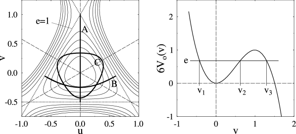
Figure 1: The Hénon-Heiles potential. Left side: equipotential lines in the $(u,v)$ plane. The dashed lines are the symmetry axes. The three shortest periodic orbits A, B, and C (evaluated at $e=1$) are shown by the heavy solid lines. Right side: scaled potential along $u=0$. (After [5].)

Hénon and Heiles [11] have already observed that the classical motion in this potential is quasi-regular up to energies $e\sim 0.5$ and then becomes increasingly chaotic; when one reaches the saddle energy ($e=1$), more than $95\%$ of the phase space is covered ergodically. The periodic orbits in the HH potential have been classified and investigated in detail by Churchill et al. [13] and more recently by Davies et al. [14]. Up to $e\simeq 0.97$ there exist only three types of periodic orbits with periods of the order of $T_{0}=2\pi$ (i.e., the fundamental period of the harmonic-oscillator potential reached in the limit $e\rightarrow 0$): the librations A and B, and the rotation C. Corresponding to the symmetry of the HH potential, orbits A and B occur in three orientations connected by rotations in the $(u,v)$ plane about $2\pi/3$ and $4\pi/3$. Orbit C maps unto itself under these rotations but has two opposite time orientations, whereas time reversal maps the orbits A and B onto themselves. The overall discrete degeneracies are thus three for orbits A and B, and two for orbit C. The orbits A are stable up to $e\simeq 0.81$ where they become unstable at a period-doubling bifurcation. At higher energies they oscillate between stability and instability, undergoing an infinite number of isochronous bifurcations that cumulate at the saddle-point energy $e=1$ where the period $T_{A}$ becomes infinity. This bifurcation cascade is the main object of our present study. For $e>1$ the orbits A do not exist any more, but a new set of three degenerate unstable librations across the saddle points come into being [13, 14, 15]; in accordance with Ref. [15] we call them $\tau$. The orbits B are unstable at all energies; the orbits C are stable at low energies and undergo a period-doubling bifurcation at the energy $e\simeq 0.89$ beyond which they remain unstable. A, B, and C are the only generic periodic orbits in the HH system for $e\leq 1$; all other orbits are created through their bifurcations (and further sequential bifurcations).

Figure 2: Oscillating part of level density of the HH potential, Gaussian averaged over an energy range $\Delta e=0.0024$, versus scaled energy $e$. Solid line: quantum-mechanical result (evaluated for $\varepsilon=0.04$). Dashed line: semiclassical result, obtained with the uniform trace formula of Ref. [6] including first and second repetitions of the three orbits A, B, and C.

In Ref. [5] the coarse-grained quantum level density of the HH potential was shown to exhibit a pronounced beating structure which could be reproduced quantitatively by Gutzwiller’s semiclassical trace formula [2] including the orbits A, B, and C. In the limit $e\rightarrow 0$, the trace formula diverges due to the approaching harmonic-oscillator limit which is integrable and has SU(2) symmetry (and a continuous two-fold degeneracy of its periodic orbits). This divergence can be removed in a uniform approximation that has recently been derived for some specific cases of SU(2) and SO(3) symmetry breaking [6]. In Fig. 2 we show a comparison of the oscillating part $\delta g(e)$ of the quantum-mechanical level density $\delta g(e)$ of the HH potential with its semiclassical approximation obtained from the uniform trace formula of Ref. [6] including only the first and second repetitions of the three orbits A, B, and C. Both results have been coarse-grained by convoluting them with a Gaussian over an energy range $\Delta e=0.0024$. The agreement is excellent up to $e\simeq 0.67$. The errors at higher energies are expected to come mainly from the orbit bifurcations that have not been taken into account (and partly from inaccuracies in the quantum result [5, 6]).

An attempt to include the bifurcations in the semiclassical approach has lead to our present study. Uniform approximations for isolated bifurcations of all generic types have been developed by Sieber and Schomerus [16] and successfully applied to the semiclassical description of various systems with mixed dynamics (see also Ref. [17] for an alternative treatment of the three simplest bifurcation types). Interferences of two close-lying bifurcations (so-called bifurcations of codimension two) were discussed in Ref. [18]. However, none of these uniform approaches can be used in the present case of the orbit A, where an infinite number of bifurcations coalesce at the saddle energy $e=1$. The uniform treatment of this bifurcation cascade in a semiclassical trace formula is a challenging task. We should mention that an infinity of orbit bifurcations in the integrable two-dimensional elliptic billiard has recently been incorporated successfully into an analytical trace formula [19]. The bifurcating orbit in the ellipse – the straight-line libration along the shorter diameter – and the orbit families created at its bifurcations are, however, of a rather simple nature, and it is not clear yet if we can apply the technique of Ref. [19] to the present system. While working along this line [20], it seemed worth while to investigate on a purely classical level the bifurcation sequence of the saddle orbit A in the HH and similar potentials, which bears a lot of resemblance to the famous Feigenbaum scenario observed in one-dimensional [21] and two-dimensional maps [22, 23]. We shall presently exhibit the self-similarity amongst the periodic orbits created at the successive bifurcations and show that it is quantitatively described by the same scaling constant $\delta$ that accounts for the geometric progression of the bifurcation energies. Different from the Feigenbaum scenario, the constant $\delta$ is given analytically here, but it is not universal in that it depends on the parameters of the potential.

A convenient method to keep track of orbit bifurcations in a two-dimensional system is to plot the trace of their stability matrix, tr M. Bifurcations occur whenever tr M $=2$. In Fig. 3 we show tr M for the primitive orbit A_n (with its Maslov index $n$ increasing by one unit at each bifurcation) and for the orbits born at its bifurcations. In the lowest panel, we see the uppermost 3% of the energy scale available for the orbit A. The first bi-

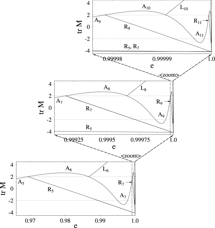
Figure 3: Trace of stability matrix M of orbit A and the orbits born at successive pitchfork bifurcations in the Hénon-Heiles potential, versus scaled energy $e$. Subscripts are Maslov indices. From bottom to top: successively zoomed energy scale near $e=1$.

furcation occurs at $e_{5}=0.969309$, where A₅ becomes unstable (with tr M_A $>2$) and a new stable orbit R₅ is born. At $e_{6}=0.986709$, orbit A₆ becomes stable again and a new unstable orbit L₆ is born. In the middle panel, we have zoomed the uppermost 3% of the previous energy scale. Here the behavior of A repeats itself, with the new orbits R₇ and L₈ born at the next two bifurcations. Zooming with the same factor to the top panel, we see the birth of R₉ and L₁₀. This can be repeated ad infinitum: each new figure will be a replica of the previous one, with all the Maslov indices increased by two units and with tr M_A oscillating forever.

Note that we have only shown here the primitives (i.e., the first repetitions) of each orbit. The higher repetitions of A will also undergo regular bifurcations and exhibit a corresponding fractal behavior. (For instance, whenever tr M of an orbit becomes equal to $-2$, its second repetition will have tr M $=2$ and bifurcate.) This infinite proliferation of stable and unstable orbits creates an increasingly mixed phase space and paves the way to chaos, similarly to the well-known Feigenbaum scenario.

We should emphasize an important difference, though, to the Feigenbaum scenario of Refs. [21, 22, 23]: the bifurcations investigated there were all period doublings. Following the new stable orbit born at each bifurcation to its next period-doubling bifurcation leads to the famous Feigenbaum tree with its fractal structure. In our present system, however, successive pitchfork bifurcations occur from one and the same orbit A. Due to the discrete symmetries of the HH potential, these bifurcations are not generic (which would imply period doubling) but they are isochronous (i.e., each new-born orbit at the bifurcation point has the same period as the parent orbit) [24]. (We have tried to follow a sequence of period-doubling bifurcations in the HH system. However, this soon leads to very long orbits that become unstable very fast with increasing energy; their investigation after more than three doublings has turned out to be numerically very difficult. Also, the successive period-doubling bifurcations are not all of pitchfork type but seem to alternate between pitchfork and touch-and-go type.)

One important result of the Feigenbaum theory was to establish the geometric progression of the bifurcation values of the system parameter through a constant $\delta$ that turned out to be universal for a certain class of maps. In the original work of Feigenbaum [21], a dissipative one-dimensional map was investigated. Successive studies in area preserving two-dimensional maps [22, 23] yielded a different value of $\delta$. Translating to the present situation, we take the energy $e$ as the system parameter and study the progression of the energy intervals $1-e_{n}$ between the cumulation point $e=1$ and the $n$-th bifurcation. Note, however, that the new orbits are born in two different sets (see Fig. 3 below): the stable rotations R_2m-1 with two time orientations, and the unstable librations L_2m that come in degenerate pairs lying symmetrically to the the saddle line containing the parent orbit ($m\geq 3$). It is thus necessary to study the corresponding sequences of bifurcations separately, so that we have to determine the ratios

$$\delta_{n}=\frac{1-e_{n}}{1-e_{n+2}}$$ (4)

separately for odd and even $n$, and to see if the values of $\delta_{n}$ become constant for large $n$. Averaging our numerical values $\delta_{n}$ from the range $7\leq n\leq 12$, we obtain $\delta_{o}=37.623$ from the odd $n$ and $\delta_{e}=37.633$ from the even $n$. The standard deviation from their mean value 37.628 is 0.082, so that the difference between $\delta_{e}$ and $\delta_{o}$ is insignificant and we may conclude that the mean value $\delta=37.628$ is unique. Below, we shall determine analytically an asymptotic value for $\delta$ which confirms this numerical result.

But let us first examine another important property of the Feigenbaum scenario for area preserving two-dimensional maps: two independent numerical constants $\alpha$ and $\beta$ were found to describe the scaling of the fixed points at the bifurcations in the two directions of the map [23]. In our Hamiltonian system, Poincaré surfaces of section – chosen through the $u$ or the $v$ axis – would provide us with two-dimensional area preserving maps and allow us to study the evolution of the fixed points with energy. However, such a study is again hampered by numerical inaccuracies. Instead, we found a geometrical self-similarity of the periodic orbits born at the bifurcations that reflects the fractal pattern of the fixed points in the Poincaré maps and can be analyzed numerically with higher accuracy.

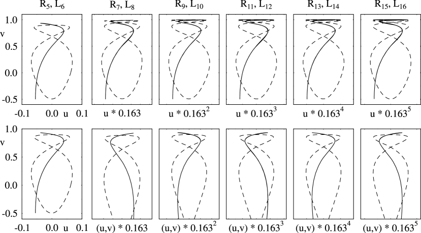
Figure 4: Orbits bifurcated from the vertical A orbit in the Hénon-Heiles potential at energy $e=1$, shown with increasing Maslov indices from left to right. Dashed lines: rotations R_2m-1, solid lines: librations L_2m ($m\geq 3$). Only one libration orbit is shown for each L_2m; its partner is obtained by reflection at the vertical symmetry line $u=0$. Top panels: successive scaling of $u$ axis from left to right with the factor 0.163. Bottom panels: successive scaling of both axes with the same factor; along the $v$ axis only the top part starting from $v=1$ is shown.

In Fig. 4 we show the shapes of the orbits born at the isochronous bifurcations of orbit A, with increasing Maslov indices from left to right; all were evaluated at the barrier energy $e=1$. We chose them here to be oriented along the $v$ axis on which their parent orbit A is lying. The closer they are born to $e=1$, the smaller has their amplitude in the transverse $u$ direction developed when they reach the barrier energy. Therefore, in the upper part of the figure, the $u$ axis has been zoomed by a factor 0.163 from each panel to the next, in order to bring the shapes to the same scale. The orbits look practically identical in the lower 97% of their vertical range, but near the barrier ($v=1$) they make one more oscillation in the $u$ direction in each generation. In the lower part of the figure, we have zoomed also the $v$ axis by the same factor from one panel to the next and plotted the top part of each orbit, starting from $v=1$. In these blown-up scales, the tips of the orbits exhibit a perfect self-similarity. The fact that the same scaling factor was used in both directions means that we find the two scaling constants $\alpha$ and $\beta$ to be identical here. We shall derive them analytically below and show how they are related to $\delta$.

Note that although the parent orbit A becomes non-compact and non-periodic for $e>1$, all periodic orbits bifurcated from it survive up to arbitrary energy, becoming more and more unstable; in spite of the non-compactness of the Hamiltonian (1) for $e>1$ they stay in a finite region of space. At $e=1$, all the orbits R_2m-1 have become inverse-hyperbolically unstable, whereas the L_2m remain direct-hyperbolically unstable. Vieira and Ozorio de Almeida [15] have also determined some of these orbits at $e>1$, both numerically and semi-analytically using Moser’s converging normal forms near a harmonic saddle. They showed, like Davies et al. [14], that with increasing energy $e>1$ these orbits come closer and closer to the librating orbits $\tau$ that oscillate across the saddles. (In Ref. [14], our orbits R₅, L₆, R₇, and L₈ were named $i_{a}$, $i_{b}$, $i_{c}$, and $i_{d}$, respectively, and $\tau$ was called S.) In Fig. 5 we present the orbits R₁₁ and $\tau$ at $e=1.00006625$, projected onto four different planes in the phase space. The mixed projections $(u,p_{u})$ and $(v,p_{v})$ correspond exactly to the results shown in Ref. [15]. Note in the upper left panel of the figure, how the R₁₁ orbit (solid line) winds around the torus of the $\tau$ orbit (dotted line).

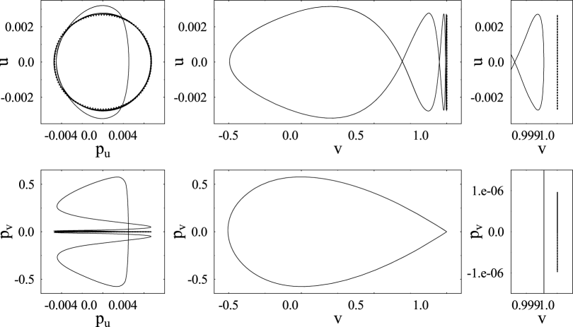
Figure 5: Periodic orbits evaluated at the energy $e=1.00006625$, projected onto four different planes in the phase space. Solid lines: orbit R₁₁, dotted lines: orbit $\tau$. Rightmost panels: zooming the $v$ and $p_{v}$ axes near the saddle point.

We shall now proceed to derive the analytical values of the scaling constants $\delta$, $\alpha$, and $\beta$. We give here only the main idea of the derivation using intuitive arguments; a more detailed mathematical analysis will be presented in a forthcoming publication [25]. The key to the understanding of the geometric progression of the bifurcation energies $e_{n}$ is a plot of tr M not versus energy $e$ but versus the period $T$. This is shown in Fig. 6. We see that for large $T$, the quantity tr M of the orbit A exhibits a perfectly periodic sinusoidal dependence on $T_{A}$ (which was noticed already in Ref. [14]). The asymptotic period of these oscillations is found here numerically to be $\Delta T=3.6276\pm 0.0003$.

This result can be analytically derived by linearizing the equations of motion (1) around the periodic orbit A which is a solution, e.g., with $u_{A}(t)=0$. The one-dimensional motion of this orbit in the $v$ direction is given by the scaled potential (cf. Fig. 1)

$$6\,V_{0}(v)=3\,v^{2}-2\,v^{3}.$$ (5)

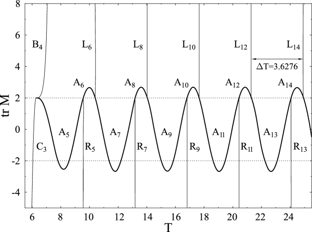
Figure 6: Trace of the stability matrix M of the orbits A (heavy line), B, C, and the orbits R_2m-1, L_2m ($m\geq 3$) born at successive pitchfork bifurcations of orbit A in the Hénon-Heiles potential, plotted versus their individual periods $T$. $\Delta T$ is the asymptotic period of the curve tr M${}_{A}\,(T_{A})$ for large $T_{A}$.

Hence we find from energy conservation

$$t\,(v)=\sqrt{3}\int_{v_{1}}^{v}\frac{ds}{\sqrt{e-3\,s^{2}+2\,s^{3}}}\,.$$ (6)

This integral can be expressed in terms of an elliptic integral of the first kind, $F$, as

$$t(v)=\sqrt{3/2}\int_{v_{1}}^{v}\frac{dv}{\sqrt{(v-v_{1})(v_{2}-v)(v_{3}-v)}}=\sqrt{6/(v_{3}-v_{1})}\,F(\gamma,k^{2})\,.$$ (7)

Hereby $v_{i}$ ($i=1,2,3$) are the zeros of the equation $6\,V_{0}(v_{i})=e$; $v_{1}$ and $v_{2}$ are the turning points of the A orbit (see Fig. 1). The arguments of the elliptic integral are

$$\gamma=\arcsin\sqrt{(v-v_{1})/(v_{2}-v_{1})}\,,\qquad k^{2}=(v_{2}-v_{1})/(v_{3}-v_{1})\,.$$ (8)

The period of the A orbit thus becomes

$$T_{A}=2\sqrt{3/2}\int_{v_{1}}^{v_{2}}\frac{dv}{\sqrt{(v-v_{1})(v_{2}-v)(v_{3}-v)}}=2\sqrt{6/(v_{3}-v_{1})}\,K(k^{2})\,,$$ (9)

where $K$ is the complete elliptic integral of the first kind which diverges when the modulus $k^{2}$ becomes unity; this happens at $e=1$ where $v_{2}=v_{3}=1$. The function $t(v)$ in (7) can be inverted in terms of the Jacobi elliptic function $\rm{sn}(s,k^{2})$ to yield the exact solution for the $v$ motion of the A orbit:

$$v_{A}(t)=v_{1}+(v_{2}-v_{1})\,\rm{sn}^{2}(s,k^{2})\,,$$ (10)

where $s$ is the scaled time variable

$$s=t\sqrt{(v_{3}-v_{1})/6}\,.$$ (11)

Linearizing Eq. (1) around the solution $u=0,\;v=v_{A}(t)$ yields the equations of motion for small perturbations $\delta u(t)$, $\delta v(t)$ around the A orbit:

$$\delta\ddot{u}(t)+[1+2v_{A}(t)]\,\delta u(t) = 0\,,$$ (12)

$$\delta\ddot{v}(t)+[1-2v_{A}(t)]\,\delta v(t) = 0\,.$$ (13)

These equations are of harmonic-oscillator type with time-periodic frequencies, usually named after Hill [26] who investigated them in connection with the lunar theory (cf. Ref. [3]). With the particular solution (10) for $v_{A}(t)$, Eq. (12) is actually a special case of the Lamé equation (see Ref. [27] for an extensive discussion of Hill’s and related equations). It is from this equation that the stability of the A orbit towards small perturbations $\delta u$ can be derived. Magnus and Winkler [27] have given an iterative scheme to solve Hill’s equation using the Fourier expansion of the time-periodic coefficient, which has been used to calculate the stability of a linear periodic orbit in the diamagnetic Kepler problem [28, 29]. We shall present the application of this procedure to the present Hamiltonian elsewhere [25], and just anticipate here that the result for tr M_A is a series

$${\rm tr\,M}_{A}\,(T_{A})=2\,\cos\,(\omega_{\perp}T_{A})+\dots\,,$$ (14)

where the dots indicate correction terms coming from the higher Fourier components of $v_{A}(t)$ in (10). All corrections have the same period $2\pi/\omega_{\perp}$ as the leading term in (14) and change therefore only the amplitude and the phase of the oscillations in tr M_A. The frequency $\omega_{\perp}$ is given by the constant term of the Fourier expansion, which equals the time average of the coefficient in (12) over the period $T_{A}$; in the limit $e\rightarrow 1$ it goes to a constant:

$$\omega_{\perp}^{2}=\langle\,[1+2\,v_{A}(t)]\;\rangle_{T_{A}}\;\longrightarrow\;3\,.$$ (15)

From this, we immediately obtain the asymptotic period

$$\Delta T=2\pi/\omega_{\perp}=2\pi/\!\sqrt{3}=3.6275987\dots$$ (16)

which is found approximately from the numerical curve tr M${}_{A}\,(T_{A})$ shown in Fig. 6.

This result can be intuitively obtained by the following reasoning. Note that the orbit A spends most of its time near the saddle point where $v=1$; this is the more true the closer the energy comes to $e=1$. Replacing $v_{A}(t)$ by its saddle-point value, the coefficient in (12) becomes $\omega_{\perp}^{2}=1+2\,v_{A}=3$. We are, in fact, just speaking in this lowest-order approximation of a harmonic oscillation transverse to the A orbit

$$\delta u(t)=u_{0}\cos\,(\omega_{\perp}t+\phi)=u_{0}\cos\,(\!\sqrt{3}\,t+\phi)\,,$$ (17)

with a constant frequency $\omega_{\perp}$ given by the curvature of the HH potential at the saddle:

$$\omega_{\perp}^{2}=\left.\partial^{\,2}V(u,v)/\partial u^{2}\right|_{u=0,v=1}=3\,.$$ (18)

Figure 7: Orbit L₁₀ evaluated at $e=1$. Right panel: shape of the orbit in the $(u,v)$ plane. Left panels: numerical results for $v(t)$ (above) and $u(t)$ (below) versus time $t$ (in steps of 0.01), shown by solid lines. Dashed line above: $v_{A}(t)$ of parent orbit A taken at the bifurcation energy $e_{10}$. Dashed line below: approximation (17) with $u_{0}=0.001017$ and the phase $\phi$ fitted to the numerical result.

In this limit, the stability matrix of the A orbit has exactly the value tr M${}_{A}\,(T_{A})=2\cos\,(\omega_{\perp}T_{A})$ (see, e.g., Ref. [10], Appendix C.2.1), in agreement with the leading term of the expansion (14). That $\delta u(t)$ is harmonic with frequency $\omega_{\perp}=\sqrt{3}$ over most of the time period $T_{A}$ is clearly seen in the results presented in Fig. 7, where we show the numerical solutions for $u(t)$ and $v(t)$ of the orbit L₁₀ evaluated at the saddle energy $e=1$. The transverse $u$ motion is, indeed, fitted extremely well over most of the period by Eq. (17) shown by a dashed line; the value of $u_{0}$ will be determined below.

The periods $T_{n}$ at which the bifurcations occur are thus given asymptotically by $T_{2m-1}\sim a+m\,\Delta T$ and $T_{2m}\sim b+m\,\Delta T$ (see Fig. 6), with $\Delta T$ given by Eq. (16) and some constants $a$, $b$. The bifurcation energies $e_{n}$ are now easily found by the asymptotic expansion of the period $T_{A}$ (9) near $e=1$, i.e., near $k^{2}=1$, where it diverges like

$$T_{A}\;\sim\;\ln\,(4/\!\sqrt{1-k^{2}})+\dots\;\sim\;\ln\,(432/\epsilon)+\dots\,,$$ (19)

with $\epsilon=1-e$. (This is easily derived from a Taylor expansion of the turning points $v_{i}$ and the quantity $k^{2}$ in powers of $\epsilon$.) Hence we find, for both even and odd $n$,

$$1-e_{n}\;\sim\;432\,e^{-T_{n}}\;\propto\;e^{-n\Delta T/2}\;\propto\;e^{-n\pi/\omega_{\perp}}\,.$$ (20)

We thus obtain with (4) the analytical value of the asymptotic energy scaling constant $\delta$

$$\delta=e^{2\pi/\omega_{\perp}}=e^{2\pi/\!\sqrt{3}}=37.622367\dots$$ (21)

which confirms the approximate numerical result given after Eq. (4).

The spatial scaling constants $\alpha$ and $\beta$ describing the self-similarity of the new periodic orbits are derived along the same lines. In the limit $v_{A}(t)=1$, the equation for $u(t)$ is harmonic even in the full equations of motion (3) and decouples from that for $v(t)$. Furthermore, the equation for $v(t)$ is of second order in $u$ so that to lowest order in small $u$ oscillations, $v(t)$ is not changed at all. Consequently, as long as the amplitude $u_{0}$ of the transverse motion $u(t)$ of the bifurcated orbits remains small, their $v$ motion is “frozen” at the bifurcation point and given by the solution $v_{A}(t)$ in (10), evaluated at $e=e_{n}$. The transverse motion $u(t)$ of the new orbit therefore carries off all the extra energy $e-e_{n}$ available above the bifurcation. That the $v$ motion of these orbits is frozen above the bifurcation energies is seen in Fig. 6 by the fact that they appear as almost vertical lines (for large enough $n$), which means that their periods are practically constant. Also, in Fig. 7 we see that $v(t)$ of the orbit L₁₀ obtained numerically at $e=1$ (solid line) is, indeed, identical to $v_{A}(t)$ evaluated at $e_{10}$ (dashed line, hardly distinguishable from the solid line). As a consequence of the frozen $v$ motion, the energy of the $u$ motion available for the new orbit at the saddle-point energy is just $1-e_{n}$. In the harmonic approximation (17), this energy is equal to

$$1-e_{n}=3\,({\dot{u}}^{2}+\omega_{\perp}^{2}u^{2})=3\,\omega_{\perp}^{2}u_{0}^{2}=9\,u_{0}^{2}\,.$$ (22)

Hence we find that the transverse amplitude of the new orbit at the saddle is given by

$$u_{0}=\sqrt{1-e_{n}}/3\,.$$ (23)

Using the numerical result $(1-e_{10})=9.305\times 10^{-6}$, the amplitude for the orbit L₁₀ becomes from the above relation $u_{0}=0.001017$ which is, indeed, the value that fits the numerical result for $u(t)$ in Fig. 7. Now, from Eq. (23) we find that the ratio of the amplitudes $u_{0}$ of two successive generations of orbits for $n\rightarrow\infty$ tends to

$$\sqrt{(1-e_{n})/(1-e_{n+2})}\;\longrightarrow\;\alpha=\sqrt{\delta}=e^{\pi/\!\sqrt{3}}.$$ (24)

This confirms the numerical scaling constant $1/\alpha=0.1630335\dots$ approximately used for the $u$ scaling in Fig. 4. The scaling constant $\beta$ for the $v$ direction, finally, is obtained from expanding the potential (5) around the barrier at $v=1$:

$$6\,V_{0}(v)=1-3\,(v-1)^{2}+\dots$$ (25)

Since the $v$ motion of the $n$th orbit is frozen, its tip near the barrier is just the turning point $v_{2}$ evaluated at $e_{n}$. Equating the frozen energy $e_{n}$ with $6\,V_{0}(v_{2})$ to leading order in (25), we find the distance $1-v_{2}$ of the tip from the saddle point to be

$$1-v_{2}=\sqrt{(1-e_{n})/3}\,.$$ (26)

Its ratio for two successive generations of orbits thus goes with $n\rightarrow\infty$ to the same limit as that found in (24) for the $u$ scaling. Hence $\beta=\alpha$, as found numerically in Fig. 4.

This concludes the derivation of our main result: the analytical value (21) of $\delta$, and the relation $\alpha=\beta=\sqrt{\delta}$. There are further interesting observations, to be interpreted in future work [25]. For large $n$ the actions of the bifurcated orbits at the saddle energy $e=1$ all tend to the action of the orbit A which is known analytically [5]: $S_{A}=6/5$. Also at $e=1$, the values for tr M of all the orbits R_2m-1 tend to the same value $-4.183$ (see their intersecting lines in Fig. 3), whereas those of the L_2m intersect at the value $+8.183$.

Finally, we add a remark about the $\tau$ orbits that exist only for $e>1$. They are oscillations transverse to the saddles (see Fig. 5, in particular the upper right panel). In the limit $e\rightarrow+1$ they become one-dimensional harmonic oscillations with the frequency $\omega_{\perp}=\sqrt{3}$. Their period is, in this limit, equal to $T_{\tau}=2\pi/\omega_{\perp}$ which is identical to $\Delta T$ in (16). Their transverse motion feels a negative curvature (corresponding to the passage over the saddle parallel to the orbit A) with the value

$$-\omega_{\parallel}^{2}=\partial^{\,2}V(u,v)/\partial v^{2}|_{u=0,v=1}=-1\,,$$ (27)

as is seen directly from Eq. (13) with $v_{A}=1$. They are therefore unstable, and their stability matrix has the trace (cf. Ref. [10], Sect. 5.6.3)

$${\rm tr}\,M_{\tau}=2\,\hbox{Cosh}\,(\omega_{\parallel}T_{\tau})=2\,\hbox{Cosh}\,(2\pi/\!\sqrt{3})\,.$$ (28)

One of the eigenvalues of M_τ is thus $\lambda=e^{2\pi/\!\sqrt{3}}$ with the Lyapounov exponent $\chi=2\pi/\!\sqrt{3}$ (or $\sigma=\chi/T_{\tau}=\omega_{\parallel}=1$). $\lambda$ is here identical with the scaling constant $\delta$ (21) for the bifurcation energies $e_{n}<1$ at which the orbits R_2m-1 and L_2m are born. This exhibits once more the intimate connection [14, 15] between the two types of periodic orbits near the threshold $e=1$, already displayed in Fig. 5.

3. Results for other two-dimensional potentials

We have investigated various two-dimensional potentials with one or more harmonic saddles and orbits that oscillate along straight lines towards the saddles. In all cases, we could find the same type of bifurcation cascades and the same self-similarity of the new-born orbits obeying the relation $\alpha=\beta=\sqrt{\delta}$. We shall give three examples below.

3.1. A simple integrable case

A separable potential with a minimum and one saddle is obtained if one omits the term proportional to $x^{2}y$ of the HH potential (1) to get

$$V(x,y)=\frac{1}{2}\,(x^{2}+y^{2})-\frac{1}{3}\,\varepsilon\,y^{3}\,,$$ (29)

and otherwise proceeds exactly in the same way as in Sect. 2. The straight-line A orbit along the $v$ axis here sees the same potential as the A orbit in the HH potential and thus has the same solution $v_{A}(t)$ given in Eq. (10). Since the potential separates in $u$ and $v$, the system is integrable. Nevertheless, the A orbit undergoes an infinite cascade of bifurcations cumulating at the energy $e=1$. The $u$ motion is strictly harmonic with period $T_{0}=2\pi$, corresponding to $\omega_{\perp}=1$, and the trace of the stability matrix of A is exactly tr M${}_{A}\,(T_{A})=2\,\cos\,(T_{A})$. The bifurcations thus occur at the periods $T_{n}=2n\pi$ with $n=1$, 2, 3, $\dots$ This leads to a scaling constant $\delta=e^{2\pi}$ for the progression of the bifurcation energies $e_{n}$. The new periodic orbits born at the bifurcations are here degenerate families with tr M $=2$ whose tips scale in $u$ and $v$ with the constant $\sqrt{\delta}=e^{\pi}$.

3.2. The Barbanis potential

Omitting the term proportional to $y^{3}$ in the HH potential yields a potential that has been studied in 1966 by Barbanis [30]:

$$V(x,y)=\frac{1}{2}\,(x^{2}+y^{2})-\varepsilon\,yx^{2}\,.$$ (30)

This potential has a minimum at $x=y=0$ and two saddles at the energy $E^{*}=1/8\varepsilon^{2}$. There are two straight-line periodic orbits A oscillating through the minimum towards the saddles. Scaling the coordinates with a factor $\varepsilon$ and rotating the coordinate system such that one of the saddle lines becomes the horizontal $u$ axis, the potential is

$$V(u,v)=\frac{1}{2}\,(u^{2}+v^{2})-\frac{1}{3\sqrt{3}}\left(2\,u^{3}-3\,uv^{2}+\sqrt{2}\,v^{3}\right).$$ (31)

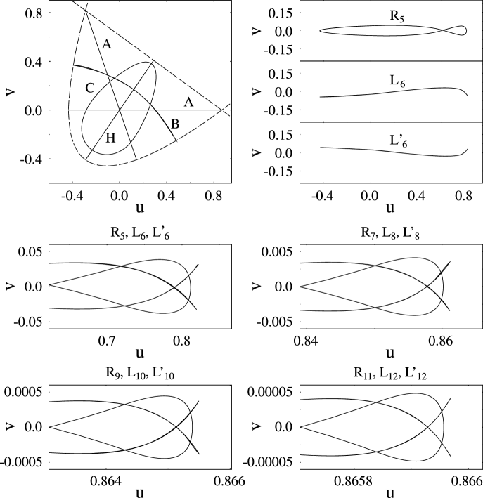
Figure 8: Periodic orbits in the potential of Barbanis [30], evaluated at the saddle-point energy $e=1$. Top panel left: primitive orbits A (in two positions), B, C, and H in the ($u,v$) plane, shown by solid lines. The dashed lines give the equipotential curves at $e=1$. Top panel right: the first generation of orbits bifurcated from the horizontal A orbit, shown on the same scale. Lower panels: extreme right tips of four generations of bifurcated orbits. The position of the saddle is at $u=\sqrt{3}/2=0.866025$ which corresponds to the right margins. The scaling factor between successive generations is 0.1084 in both directions.

Fig. 8 shows the primitive periodic orbits in this potential. In the top left panel, we see the equipotential curves for $e=E/E^{*}=1$ by dashed lines: they form a parabola and a straight line intersecting at the two saddles. The solid lines indicate the shortest periodic orbits evaluated here at $e=1$. Note that the two straight saddle lines that contain the A orbits are no symmetry axes (in contrast to the HH potential). The potential (31) has only one symmetry line which halves the angle between the saddle lines and contains a straight-line librating orbit H₄ that is unstable at all energies. There is one curved librating orbit B₄ that oscillates transverse to the symmetry axis and is also unstable at all energies (like the orbits B in the HH potential). C is a rotating orbit that remains stable up to $e=2.415$. The orbits A have the same behavior as in the HH potential and create an infinite set of new orbits at isochronous pitchfork bifurcations.

Since the potential is not symmetric about the saddle lines, the new libration orbits born at the bifurcations come in pairs with equal Maslov indices $2n$ but shapes, actions and stabilities that differ at energies $e>e_{2n}$; we call them here L_2n and L’_2n. The new rotations R_2n-1 again have two time orientations and thus a discrete degeneracy of two. The shapes of these new orbits resemble much those in the HH potential (apart from the asymmetry of the unstable pairs). Their self-similarity is shown in the lower four panels of Fig. 8, where their tips close to the saddle point $u=\sqrt{3}/2$ are displayed for each generation. The panels from each generation to the next are scaled by a factor 0.1084 both in $u$ and $v$ direction. The bifurcation energies $e_{n}$ are again found to cumulate in a geometric progression, with a numerical scaling constant $\delta=85.1\pm 0.5$.

The values of tr M of all the primitive orbits are shown in Fig. 9 as functions of their period $T$. We find again a periodic behavior of tr M${}_{A}\,(T_{A})$, here with period $\Delta T=4.443$.

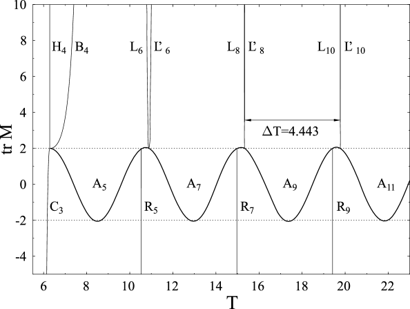
Figure 9: Trace of stability matrix M of orbits A (heavy line), B, C, H, and the new orbits born at successive pitchfork bifurcations of orbit A in the Barbanis potential, plotted versus their individual periods $T$.

The analytical values of these constants are found exactly in the same way as for the HH potential. In fact, the one-dimensional barrier seen by the A orbits in the Barbanis potential is, apart from a trivial scaling factor $\sqrt{3}/2$, identical to that in the HH potential. The frequency of the transverse oscillations across the saddles here is found to be $\omega_{\perp}=\sqrt{2}$, so that $\Delta T=\sqrt{2}\pi=4.4428829\dots$ , and the scaling constant $\delta$ of this potential becomes

$$\delta=e^{\sqrt{2}\pi}=85.019695\dots$$ (32)

The scaling constants for the self-similar tips of the periodic orbits are therefore

$$\alpha=\beta=\sqrt{\delta}=1/0.10845266\dots$$ (33)

Both these values confirm the numerically determined constants.

3.3. The quartic Hénon-Heiles potential

In Refs. [6, 31] a quartic Hénon-Heiles potential was investigated that has a four-fold discrete rotational symmetry and four saddle points. It is given, in scaled coordinates, by

$$V(u,v)=\frac{1}{2}\,(u^{2}+v^{2})-\frac{1}{4}\,(u^{4}+v^{4})+\frac{3}{2}\,u^{2}v^{2}\,.$$ (34)

We refer to the above literature for a discussion of the shortest periodic orbits (which we have renamed here to simplify the notation). We show the equipotential curves and the orbits A, B, and C in the top left panel of Fig. 10. The orbits A have the same behavior as those in the standard HH potential, except that they oscillate between two opposite saddle points. They undergo again an infinite series of isochronous pitchfork bifurcations. The difference to the standard HH case is that here the nature of the new orbits born at the bifurcations alternates between rotations R_n and librations L${}_{n^{\prime}}$ also amongst the stable orbits (odd $n$) and the unstable orbits (even $n$), as is shown for the orbits R₅, L₆, L₇, and R₈ labeled explicitly in Fig. 10. As a consequence, the self-similarity of their tips near the saddles becomes apparent only over two generations. Correspondingly, each of the lower four panels contains the tips of two successive generations of orbits, and the scaling from one panel to the next is done with the factor $\alpha^{2}=\beta^{2}=\delta$. The frequency of the small oscillations across the saddles here is $\omega_{\perp}=2$, and the period of tr M${}_{A}\,(T_{A})$ becomes asymptotically $\Delta T=2\pi/\omega_{\perp}=\pi$. The expansion of $T_{A}$ near the saddle energy gives here, with $\epsilon=1-e$,

$$T_{A}\;\sim\;\sqrt{2}\,\ln\,(64/\epsilon)+\dots$$ (35)

For the bifurcation energies $e_{n}$ we have thus asymptotically (note the extra factor $\sqrt{2}$)

$$1-e_{n}\;\sim\;64\,e^{-T_{n}/\!\sqrt{2}}.$$ (36)

With $T_{n}\sim n\pi/\omega_{\perp}=n\pi/2$, we find for the energy scaling constant

$$\delta=e^{\pi/\!\sqrt{2}}=9.2206125\dots$$ (37)

Its inverse is $1/\delta=1/\alpha^{2}=0.108452664\dots$ , i.e., the scaling factor used in Fig. 10.

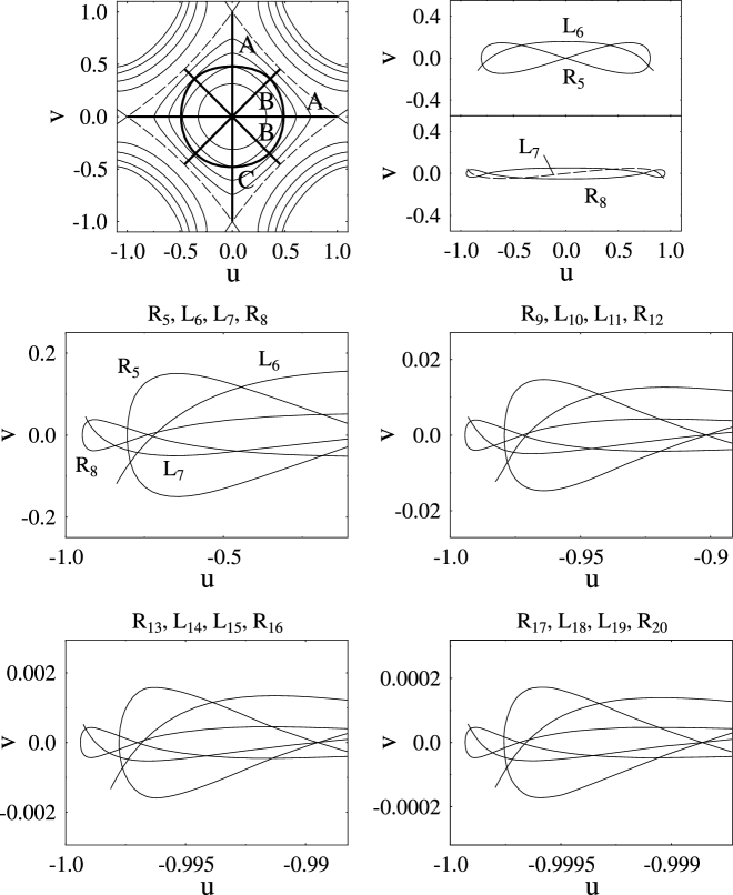
Figure 10: Periodic orbits in the quartic Hénon-Heiles (HH4) potential, evaluated at $e=1$. Upper left panel: equipotential curves (thin lines; dashed for $e=1$) and the primitive orbits A, B, and C (heavy lines). Upper right panel: the first two generations of bifurcated horizontal orbits R₅, L₆ (above) and L₇, R₈ (below; orbit L₇ is dashed), drawn on the same vertical and horizontal scales as the orbits in the upper left panel. Lower four panels: Tips of the bifurcated orbits R₅ - R₂₀ near the left saddle ($u=-1)$, plotted on increasingly zoomed scales. The scaling factor from each pair of generations to the next is 0.10845 in both directions.

The numerical iteration of the bifurcation energies $e_{n}$ was easier in this potential. The average value of the $\delta_{n}$ given by Eq. (4) in the range $7\leq n\leq 16$ gives a mean value of $\delta=9.2203$ with a standard deviation of 0.02. The asymptotic value of $\Delta T=\pi$ is reached for the interval $T_{19}-T_{17}$ with an accuracy of 7 digits.

4. Summary and conclusions

We have investigated cascades of isochronous pitchfork bifurcations of straight-line librational orbits in the Hénon-Heiles and similar two-dimensional potentials possessing one or more harmonic saddles. The bifurcation energies cumulate at the saddle-point energy (scaled to be $e=1$); their geometric progression yields a scaling constant $\delta$ that can be calculated analytically in terms of the potential parameters. The periodic orbits born at the successive bifurcations exhibit a self-similarity corresponding to scaling constants $\alpha$ and $\beta$ in the two spatial directions that turn out to be identical and equal to $\alpha=\beta=\sqrt{\delta}$.

This result applies to a whole class of Hamiltonian systems with harmonic saddles and straight-line librational orbits oscillating towards the saddle points. The trace of the stability matrix of these orbits as a funcion of their period $T_{A}$, tr M ($T_{A}$), oscillates with an asymptotic periodicity $\Delta T=2\pi/\omega_{\perp}$, where $\omega_{\perp}^{2}$ is the transverse curvature at the saddles, see Eq. (18). Combining this with the asymptotic energy dependence $T_{A}\sim d\ln[c/(1-e)]$, one finds the asymptotic values $e_{n}$ of the bifurcation energies. From those, the analytic form of the scaling constant $\delta$ in terms of the parameters $\omega_{\perp}$ and $d$ is found to be $\delta=e^{2\pi/\omega_{\perp}d}$. The Lyapounov exponent of the new unstable orbits $\tau$ librating across the saddles for $e>1$ is, in the limit $e\rightarrow+1$, given by $\chi=2\pi\omega_{\parallel}/\omega_{\perp}$ (or $\sigma=\chi/T_{\tau}=\omega_{\parallel}$), where $-\omega_{\parallel}^{2}$ is the negative parallel curvature at the saddles, see Eq. (27).

The well-known Feigenbaum scenario in two-dimensional area preserving maps [22, 23] differs from that studied here in three respects. First, the bifurcations discussed there are successive period-doublings which form a fractal tree. Second, their constants $\delta$, $\alpha$, and $\beta$ are all different from each other and only known numerically. Third, these constants appear to be universal for a whole class of quadratic maps, whereas in the present case the constant $\delta$ depends explicitly on the parameters of the potential. We should bear in mind that the Poincaré maps corresponding to the Hamiltonian systems studied here are, of course, no simple quadratic maps.

An isochronous pitchfork bifurcation cascade of a linear periodic orbit has been found also in the diamagnetic Kepler problem [29, 32]. This orbit does not approach a saddle point but becomes infinitely long in the limit $E\rightarrow-\,0$ where its bifurcations cumulate. The self-similarity of the periodic orbits born at the bifurcations has not been investigated; the progression of the bifurcation energies is easily found to yield the constant $\delta=1$ (cf. Refs. [33, 34]). The same value $\delta=1$ is also found for the bifurcations of the short diameter orbit in the ellipse billiard, which are $m$-uplings with $m\geq 2$ cumulating in the limit $m\rightarrow\infty$ at zero excentricity (cf. Ref. [19] and Ref. [10], problem 5.3).

It will be interesting to study also the modifications arising in connection with non-harmonic saddles, or with curved librating orbits approaching a saddle.

Acknowledgments

I am very grateful to Mitaxi Mehta for illuminating discussions and a critical reading of the manuscript, and to Kaori Tanaka for considerable improvements of our numerical POT code in an ongoing collaboration [12]. I also acknowledge encouraging discussions with S. Fedotkin, J. Kaidel, A. Magner, M. V. N. Murthy, J. M. Rost, and M. Sieber.

Note added in proof:

The transverse motion $u(t)$ [or $v(t)$ in Sects. 3.2 and 3.3] of the bifurcated orbits R_n, L_n is given, close enough to their bifurcation energies so that its amplitude remains small, by the periodic Lamé functions¹ Ec${}_{p}^{m}(at)$ and Es${}_{p}^{m}(at)$. Hereby $m$ is the number of zeros that can be uniquely related to the Maslov index $n$, and $p$ and $a$ are fixed numbers that depend on the potential. We find that the trigonometric expansions of Ec${}_{p}^{m}(z)$ and Es${}_{p}^{m}(z)$ given in Erdélyi et al. reproduce our numerical results to a high degree of accuracy (see Ref. [25] for details).

¹see, e.g., Higher Transcendental Functions, Vol. III, A. Erdélyi et al., eds. (McGraw-Hill, New York, 1955), Chapter XV.

References

- [1]
- [2] M. C. Gutzwiller, J. Math. Phys. 12, 343 (1971).
- [3] M. C. Gutzwiller: Chaos in classical and quantum mechanics (Springer, New York, 1990).
- [4] V. M. Strutinsky, Nukleonika (Poland) 20, 679 (1975); V. M. Strutinsky and A. G. Magner, Sov. J. Part. Nucl. 7, 138 (1976); V. M. Strutinsky, A. G. Magner, S. R. Ofengenden, and T. Døssing, Z. Phys. A 283, 269 (1977).
- [5] M. Brack, R. K. Bhaduri, J. Law, and M. V. N. Murthy, Phys. Rev. Lett. 70, 568 (1993); M. Brack, R. K. Bhaduri, J. Law, Ch. Maier, and M. V. N. Murthy, Chaos 5, 317 (1995); ibid. (Erratum) 5, 707 (1995).
- [6] M. Brack, P. Meier, and K. Tanaka, J. Phys. A 32, 331 (1999).
- [7] S. M. Reimann, M. Persson, P. E. Lindelof, and M. Brack, Z. Phys. B 101, 377 (1996).
- [8] J. Blaschke and M. Brack, Europhys. Lett. 50, 294 (2000).
- [9] M. Brack, S. M. Reimann, and M. Sieber, Phys. Rev. Lett. 79, 1817 (1997); M. Brack, P. Meier, S. M. Reimann, and M. Sieber, in: Similarities and differences between atomic nuclei and clusters, eds. Y. Abe et al. (A.I.P., 1998) p. 17; M. Brack, M. Sieber, and S. M. Reimann, in: Quantum Chaos Y2K, Proceedings of Nobel Symposium 116, K.-F. Berggren and S. Åberg (Eds.), Physica Scripta Vol. T90 (2001), 146. First steps towards the inclusion of spin-orbit interactions are reported in M. Brack and Ch. Amann, in: Fission Dynamics of Atomic Clusters and Nuclei, eds. D. Brink et al. (World Scientific Publishing, 2001), in print.
- [10] M. Brack and R. K. Bhaduri: Semiclassical Physics, Frontiers in Physics, Vol. 96 (Addison-Wesley, Reading, USA, 1997).
- [11] M. Hénon and C. Heiles, Astr. J. 69, 73 (1964).
- [12] K. Tanaka and M. Brack, to be published.
- [13] R. C. Churchill, G. Pecelli, and D. L. Rod, in Stochastic Behavior in Classical and Quantum Hamiltonian Systems, ed. by G. Casati and J. Ford (Springer-Verlag, N.Y., 1979) p. 76.
- [14] K. T. R. Davies, T. E. Huston, and M. Baranger, Chaos 2, 215 (1992).
- [15] W. M. Vieira and A. M. Ozorio de Almeida, Physica D 90, 9 (1996).
- [16] M. Sieber, J. Phys. A 29, 4715 (1996); H. Schomerus and M. Sieber, J. Phys. A 30, 4537 (1997); M. Sieber and H. Schomerus, J. Phys. A 31, 165 (1998).
- [17] J. Main and G. Wunner, Phys. Rev. A 55, 1743 (1997).
- [18] H. Schomerus, Europhys. Lett. 38, 423 (1997); J. Phys. A 31, 4167 (1998).
- [19] A. Magner, S. N. Fedotkin, K. Arita, T. Misu, K. Matsuyanagi, T. Schachner, and M. Brack, Prog. Theor. Phys. (Japan) 102, 551 (1999).
- [20] A. Magner, S. N. Fedotkin, and M. Brack, work in progress.
- [21] M. J. Feigenbaum, J. Stat. Phys. 19, 25 (1978); see also M. J. Feigenbaum, Physica 7 D, 16 (1983).
- [22] T. C. Bountis, Physica 3 D, 577 (1981).
- [23] J. M. Greene, R. S. McKay, F. Vivaldi, and M. J. Feigenbaum, Physica 3 D, 468 (1981).
- [24] The non-generic nature of the bifurcations in potentials with discrete symmetries has been discussed, e.g., by M. A. M. de Aguiar, C. P. Malta, M. Baranger, and K. T. R. Davies, Ann. Phys. (N.Y.) 180, 167 (1987), and by Mao and Delos [29].
- [25] S. Fedotkin, M. Mehta, K. Tanaka, and M. Brack, to be published.
- [26] G. W. Hill, Acta Math. 8, 1 (1886).
- [27] W. Magnus and S. Winkler: Hill’s Equation (Interscience Publ., New York, 1966).
- [28] A. R. Edmonds, J. Phys. A 22, L673 (1989).
- [29] J.-M. Mao and J. B. Delos, Phys. Rev. A 45, 1746 (1992).
- [30] B. Barbanis, Astr. J. 71, 415 (1966).
- [31] M. Brack, S. C. Creagh, and J. Law, Phys. Rev. A 57, 788 (1998).
- [32] J. Main, G. Wiebusch, A. Holle, and K. H. Welge, Phys. Rev. Lett. 57, 2789 (1986).
- [33] M. Y. Sumetskii, Sov. Phys. JETP 56, 959 (1983).
- [34] J. Main, G. Wiebusch, A. Holle, and K. H. Welge, Z. Phys. D 6, 295 (1987).