[

Shear Effects in Non-Homogeneous Turbulence

Abstract

Motivated by recent experimental and numerical results, a simple unifying picture of intermittency in turbulent shear flows is suggested. Integral Structure Functions (ISF), taking into account explicitly the shear intensity, are introduced on phenomenological grounds. ISF can exhibit a universal scaling behavior, independent of the shear intensity. This picture is in satisfactory agreement with both experimental and numerical data. Possible extension to convective turbulence and implication on closure conditions for Large-Eddy Simulation of non-homogeneous flows are briefly discussed.

PACS: 47.27-i, 47.27.Nz, 47.27.Ak ]

Statistical properties of turbulent flows are usually characterized in terms of the scaling behavior of velocity Structure Functions (SF). These quantities are defined as the statistical moments of longitudinal velocity increments across a separation $r$ at the location $x$: ${D}_{p}(\mbox{\mbox{\boldmath$x$}},{\mbox{\mbox{\boldmath$r$}}})=\left\langle\delta v(\mbox{\mbox{\boldmath$x$}},{\mbox{\mbox{\boldmath$r$}}})^{p}\right\rangle$. In homogeneous and isotropic turbulence, ${D}_{p}(\mbox{\mbox{\boldmath$x$}},{\mbox{\mbox{\boldmath$r$}}})$ only depends on the distance (or scale) $r$. Experimental and numerical observations support the idea that ${D}_{p}(r)$ display universal power-law dependence on $r$ in the so-called inertial range, i.e. ${D}_{p}(r)\sim r^{\zeta_{p}}$. Universality refers here to the scaling exponents $\zeta_{p}$ being independent of the stirring process of turbulence. The $\zeta_{p}$ values are found to be in disagreement with Kolmogorov’s linear prediction (K41) $\zeta_{p}=p/3$ [1]. The understanding of this correction to K41, usually referred to as intermittency, has stimulated many phenomenological and theoretical works during the last 40 years (see [2] for a recent review).

Only recently, interests in understanding intermittency in non-homogeneous turbulent flows have started to emerge (see [3, 4, 5, 6, 7, 8, 9, 10]). The major point is to understand how the phenomenology of intermittency is modified, or can be extended, in case of non-homogeneous flows. A common characteristic of such flows, e.g. wall-bounded flows, is the presence of a non-zero mean velocity gradient (usually called shear). Note that shear does not necessarily imply inhomogeneity, e.g. in homogeneous shear, straining and rotational flows.

Our investigation starts from the following key observations: i) In presence of a strong shear, intermittency, defined as the deviation of scaling exponents $\zeta_{p}$ from the linear law, is larger than in homogeneous and isotropic turbulence. ii) Relative scaling exponents, measured in very different flows but in positions where the shear is strong enough, seems to be very similar (universal).

Data in Fig. 1 fully confirm our two key observations. They come from very different situations: near the wall in a channel flow numerical simulation [4, 5] and experiment [6], in the logarithmic sublayer of a boundary layer flow [7], near a strong vortex [8], in the wake of a cylinder [9] and in a Kolmogorov flow [10].

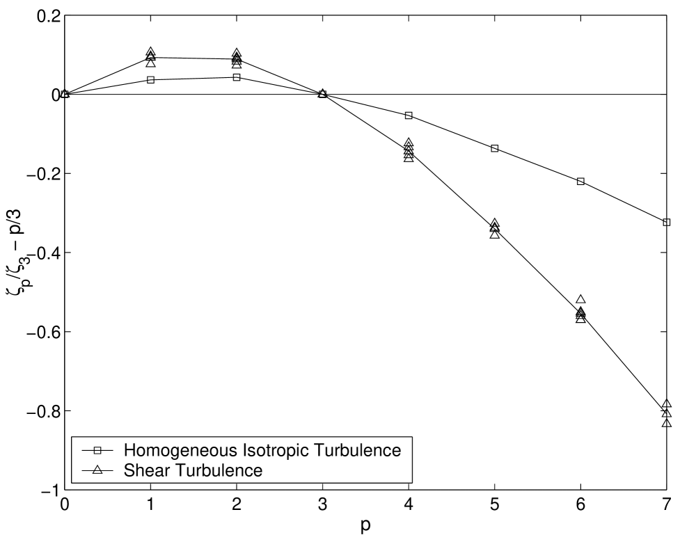
FIG. 1.: Intermittency corrections to scaling exponents, $\zeta_{p}/\zeta_{3}-p/3$, in homogeneous and isotropic turbulence ($\Box$), and several turbulent shear flows ($\triangle$). Intermittency corrections are significantly larger in presence of shear and display universality.

In order to provide a theoretical unifying framework for non-homogeneous turbulent shear flows, we start from the Navier-Stokes (N-S) equations. The velocity field can be decomposed into a mean value (average is meant on time) plus a fluctuating part: ${\mbox{\mbox{\boldmath$v$}}}(\mbox{\mbox{\boldmath$x$}};t)={\overline{{\mbox{\mbox{\boldmath$v$}}}}}(\mbox{\mbox{\boldmath$x$}})+{\mbox{\mbox{\boldmath$v$}}}^{\prime}(\mbox{\mbox{\boldmath$x$}};t)$. It yields the usual Reynolds decomposition

$$D_{t}v^{\prime}_{i}+{\cal S}_{ij}(\mbox{\mbox{\boldmath$x$}})v^{\prime}_{j}+v_{j}^{\prime}\partial_{j}v^{\prime}_{i}-{\overline{v_{j}^{\prime}\partial_{j}v^{\prime}_{i}}}=-\partial_{i}p^{\prime}+\nu\Delta v^{\prime}_{i}$$ (1)

with $D_{t}=\left(\partial_{t}+{\overline{v}}_{j}\partial_{j}\right)$. The shear is defined as ${\cal S}_{ij}\left(\mbox{\mbox{\boldmath$x$}}\right)=\partial_{j}{\overline{v}_{i}\left(\mbox{\mbox{\boldmath$x$}}\right)}$ and will depend on the mean flow geometry. In regions where ${\cal S}_{ij}=0$, e.g. very far from the boundaries, turbulence can be considered as homogeneous. Otherwise, the shear term ${\cal S}_{ij}(\mbox{\mbox{\boldmath$x$}})v^{\prime}_{j}$ must be taken into account. The results displayed in Fig. 1 show that the presence of this term modifies significantly the statistical properties of turbulence. In order to better hilight the physical implication of the shear, we consider together the second and third terms of the l.h.s. of (1), defining the following Integral Structure Functions (ISF):

$${\tilde{D}}_{p}(z,r)=\left\langle\left(\delta v(z,r)^{3}+\alpha r\cdot{\cal S}(z)\cdot\delta v(z,r)^{2}\right)^{p/3}\right\rangle,$$ (2)

where $\alpha$ is an empirical prefactor of order one. These ISF are expected to take into account shear effects, particularly at large scales (see next paragraph) and to display a universal behavior. We consider here generic situations in which the shear reduces to ${\cal S}(z)=\partial_{z}{\overline{v}_{x}}$. Such situation occurs near a rigid wall, where the principal mean-velocity component aligns in the $x$-direction, parallel to the boundary [11]. The shear ${\cal S}(z)$ characterizes the variation of $v_{x}$ along the $z$-direction, i.e. as one moves off the wall. Finally, we consider increments in the direction of the mean flow, i.e. orthogonal to the shear direction.

ISF reduce on two different SF when either the first or the second term dominates. These two terms will exactly balance at scale $L_{{\cal S}}$ such that ${{\delta v(L_{{\cal S}})}/{L_{{\cal S}}}}=\alpha~{}{\cal S}.$ At scales $r\ll L_{{\cal S}}$, shear effects become negligible and homogeneous and isotropic scalings are expected. Kolmogorov’s scaling then yields $\delta v(r)\sim\epsilon^{1/3}r^{1/3}$, where $\epsilon$ denotes the mean energy dissipation rate. By extending this similarity relation to the scale $r=L_{{\cal S}}$, one obtains the usual dimensional estimate for the shear length scale $L_{{\cal S}}\sim\left(\epsilon/{\cal S}^{3}\right)^{1/2}$ [12]. In the logarithmic layer of a plane near-wall flow it yields $L_{\cal S}(z)\sim z$ [7]. Roughly speaking, $L_{{\cal S}}$ can be viewed as the size of small-scale eddies, whose turn-over time equals the shear time scale $1/{\cal S}$, imposed by the flow geometry and the stirring process of turbulence at large scales. Note that this estimate of the shear length-scale stems out from dimensional analysis. In practice, there may be a prefactor in the expression of $L_{s}$: this is taken into account by the coefficint $\alpha$. From previous reasoning it follows that ${\tilde{D}}_{p}(r)\sim{D}_{p}(r)$ for $r\ll L_{s}$ and ${\tilde{D}}_{p}(r)\sim\left(r{\cal S}\right)^{p/3}{D}_{2p/3}(r)$ for $r\gg L_{s}$.

Another way to see that the central objects, in presence of shear, are the ISF, comes from the generalization of Yaglom’s equation to homogeneous-shear flows, i.e. with ${\cal S}(z)={\cal S}$ [12, 13]:

$$-{4\over 5}\epsilon r = {D}_{3}(r)-6\nu{{d~{}{D}_{2}(r)}\over{dr}}+$$ (3)

$$- {2{\cal S}\over{r^{4}}}\int^{r}_{0}{dx\;x^{4}\;\overline{v_{x}^{\prime}(x_{0})\cdot v_{z}^{\prime}(x_{0}+x)}}.$$ (4)

Supposing that this relation can be generalized, along the same line of idea of the Kolmogorov’s Refined Similarity Hypothesis [14], one obtains

$$\delta v^{3}(r)+\alpha r\cdot{\cal S}\cdot\overline{v_{x}^{\prime}(x)\cdot v_{z}^{\prime}(x+r)}\sim\varepsilon(r)\cdot r,$$ (5)

where $\varepsilon(r)$ denotes the coarse-graining of the energy dissipation field $\epsilon=\frac{\nu}{2}\sum_{i,j}\left(\partial_{i}v_{j}\right)^{2}$, at scale $r$.

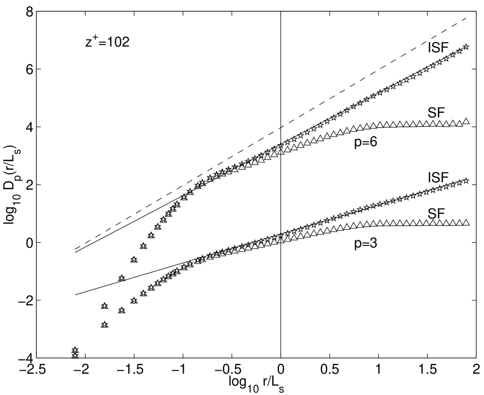
FIG. 2.: In the turbulent boundary layer at the distance $z^{+}=102$. ${D}_{3}$ and ${D}_{6}$ ($\triangle$) are compared with ${\tilde{D}}_{3}$ and ${\tilde{D}}_{6}$ ($\star$). The scale $r$ has been renormalized by the characteristic shear length-scale $L_{s}$. The solid lines passing through ${\tilde{D}}_{3}$ and ${\tilde{D}}_{6}$ indicate the expected homogeneous and isotropic power-laws, respectively $\zeta_{3}=1$ and $\zeta_{6}=1.78$. For comparison, the dashed line has slope $2$.

Simplifying, on pure dimensional grounds, the velocity-cross correlation $\overline{v_{x}^{\prime}v_{z}^{\prime}}$, with $\delta v(r)^{2}$ one ends up again with ${\tilde{D}}_{p}(r)$. Furthermore, we propose the following Refined Similarity Hypothesis

$${\tilde{D}}_{p}(r)=\left\langle\left(\delta v(r)^{3}+\alpha r\cdot{\cal S}\cdot\delta v(r)^{2}\right)^{p/3}\right\rangle\sim\left\langle\varepsilon(r)^{p/3}\right\rangle r^{p/3}.$$

This formulation is consistent, in the limiting cases of strong and negligible shear, with some recent findings (see [4, 5]). In addition to that, the ISF should be able to abridge smoothly between these two limiting regimes, i.e.

$$r\ll L_{{\cal S}}\; : \;\;\;\;{D}_{p}(r)\sim\left\langle\varepsilon(r)^{p/3}\right\rangle\cdot r^{p/3}$$ (6)

$${\rm and}\;\;\;\;r\gg L_{{\cal S}}\; : \;\;\;\;{D}_{p}(r)\sim\left\langle\varepsilon(r)^{p/2}\right\rangle.$$ (7)

Eqn. (6) is in agreement with the restoration of homogeneity and isotropy at small scales. For $r\gg L_{{\cal S}}$, eqn. (7) gives ${D}_{2}(r)\sim const$ (modulo possible logarithmic corrections), yielding for the energy spectrum $E(k)\sim k^{-1}$ (a relation suggested long time ago in [12]).

In the previous picture, it is assumed that the shear length scale $L_{\cal S}$ remains larger than the dissipation length scale $\eta$. The dissipation field $\varepsilon(r)$ is then expected to display the same scaling properties as in homogeneous and isotropic turbulence. However, in regions where $L_{\cal S}\lesssim\eta$ (very close to the wall) it is expected that shear effects act down to the dissipative scale and therefore can modify the scaling behavior of $\varepsilon(r)$. The scalings of ${D}_{p}(r)$ should then also change according to (7).

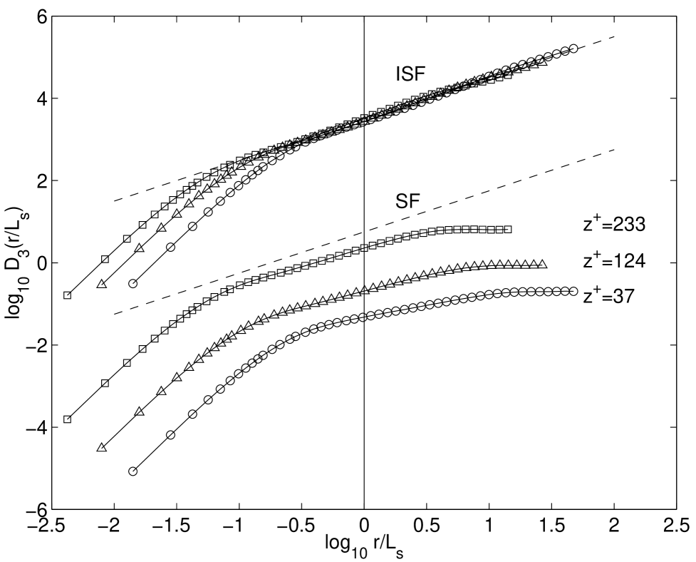
FIG. 3.: From the boundary layer experiment, third-order structure function at various distances from the wall: $z^{+}=37$ ($\circ$), $z^{+}=124$ ($\triangle$) and $z^{+}=233$ ($\Box$). The scaling properties of ${D}_{3}$ (SF) do depend on the distance $z^{+}$. On the contrary, ${\tilde{D}}_{3}$ (ISF) displays the same scaling behavior for all $z^{+}$. The dashed line has slope $1$. The curves have been shifted vertically for convenience.

The relevance of Integral Structure Functions for describing the scaling properties of non-homogeneous shear flows is now tested on both experimental and numerical data. The experiment, performed in the recirculating wind tunnel of ENS-Lyon, consists in a turbulent boundary-layer flow over a smooth horizontal plate (see [7] for details about the experimental apparatus). Velocity measurements are carried out at various elevations from the plate in the logarithmic turbulent sublayer [11]. Numerical results are obtained from a direct simulation of the Navier-Stokes equations in a rectangular channel flow (see [4] for details).

In Fig. 2, ${D}_{3}$ and ${D}_{6}$, measured in the logarithmic boundary sublayer, are compared with the corresponding ${\tilde{D}}_{3}$ and ${\tilde{D}}_{6}$. The shear ${\cal S}(z)=\partial_{z}{\overline{v}_{x}}$ has been estimated from the mean velocity profile. In standard non-dimensional variables [15], namely $z^{+}=v_{*}z/\nu$ and $v^{+}=\bar{v}_{x}/v_{*}$ where $v_{*}$ is the characteristic velocity of the viscous sublayer, our data are well fitted by the logarithmic profile $v^{+}(z^{+})={(1/{\kappa})}\log(z^{+})+B$. We obtain $\kappa\simeq 0.4$ and $B\simeq 5.26$ in agreement with previously reported results [7]. For what concerns the coefficient $\alpha$, all our results have been obtained with the fixed value $\alpha\approx 0.2$. Note that the constant $\alpha$ is not (a priori) intended to be universal but may strongly depend on the geometry and stirring process of the flow. However, it is expected to remain of order unity. In practice, the value of $\alpha$ has been extracted from data by requiring that one third-order ISF scale as $r$ (see next paragraph). Corresponding estimates of $L_{s}$ are indicated in all figures. Finally, one must point out that velocity increments have been estimated in the direction of the mean flow by use

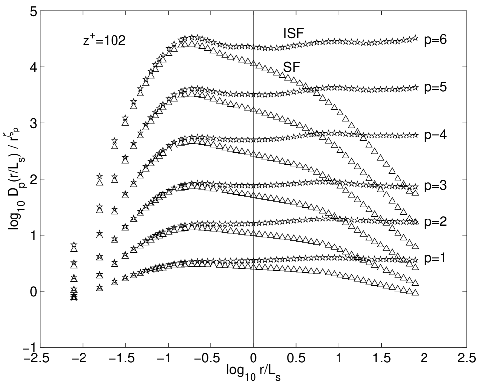
FIG. 4.: In the experimental boundary layer at $z^{+}=102$. SF and ISF, compensated by homogeneous and isotropic scalings, are displayed for p=$1\dots 6$.

of the Taylor hypothesis. Both ${D}_{3}$ and ${D}_{6}$ exhibit a power-law dependence on $r$ but the scaling exponents are clearly different from those observed in homogeneous and isotropic (h-i) turbulence, respectively, $\zeta_{3}\simeq 1$ and $\zeta_{6}\simeq 1.78$. On the other hand, the corresponding ISF exhibit power-laws in good agreement with h-i scalings (up to very large scales).

In Fig. 3, third-order SF and ISF are displayed for various distances from the wall. We notice that scaling behavior of ${D}_{3}$ changes with $z^{+}$. On the contrary, all the corresponding ${\tilde{D}}_{3}$ display the same power-law scaling with exponent $1$. We recall that the coefficient $\alpha$ is kept constant and the shear is estimated from the mean velocity profile; there is no adjustable parameter.

We now report a sharper test: SF and ISF, compensated by h-i power-law scalings, are displayed in Fig. 4 for $p=1,\dots,6$ at distance $z^{+}=102$. A departure from h-i scalings is clearly observed for SF.

On the contrary, ${\tilde{D}}_{p}(r)/r^{\zeta_{p}}$ exhibits a plateau up to very large scales, indicating that ISF roughly behave as $r^{\zeta_{p}}$. In other terms, ISF compensate shear effects and restore, via the extra term $\alpha r\cdot{\cal S}\cdot\delta v(r)^{2}$, the h-i scalings. Finally, the same test, made on numerical data, is reported in Fig. 5 for the sake of comparison. Data are obtained at distance $z^{+}=25$ from the wall, i.e. where the shear is strong. Results are in reasonable agreement with those of Fig. 4, despite the lower resolution of the numerical simulation. We would like to underline the major points of our study. Our description relates the scaling properties of velocity fluctuations in non-homogeneous shear flows, to those of the coarse-grained dissipation rate $\varepsilon(r)$. Provided that the shear length-scale remains much larger than the dissipative length-scale, we are inclined to believe that the scaling properties of $\varepsilon(r)$ remain flow-independent; the dissipation process, operating on very

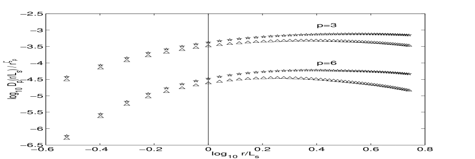
FIG. 5.: As in Fig. 4 but from numerical data at $z^{+}=25$.

small-scales, is mainly insensitive to the presence of the shear. We then claim that the scalings of velocity fluctuations are different in sheared regions only because the similarity between $\delta v(r)$ and $\varepsilon(r)$ changes form (see (6) and (7)). When $L_{S}\lesssim\eta$, shear effects acting down to dissipative scales are expected to modify the scaling behavior of $\varepsilon(r)$. Nonetheless, we observe in Fig. 1 that relative scalings exponents of velocity structure functions remain universal.

The introduction of ISF relies on quite simple dimensional arguments. However, they have proved to be valuable (preliminary) tools in order to capture (at leading order) shear effects on the scaling behavior of velocity structure functions. We believe that some refinements in the definition of ISF may be possible, e.g. considering the cross correlation $\overline{v_{x}^{\prime}v_{z}^{\prime}}$ instead of $\delta v(r)^{2}$: however ISF are of practical interest as they are easily accessible experimentally.

A possible extension of ISF applies to thermal turbulent convection, the buoyancy term $ag\delta T(r)$ playing a similar role of ${\cal S}\cdot\delta v(r)$. In that case, the ISF would read

$${\tilde{D}}^{\mbox{RB}}_{p}(r)=\left\langle\left(\delta v(r)^{3}+\alpha r\cdot ag\delta T(r)\cdot\delta v(r)\right)^{p/3}\right\rangle$$

and are expected to take into account buoyancy effects at scales larger than the Bolgiano length-scale.

An important application of our findings concerns Large Eddy Simulations (LES). Usual eddy viscosity models are known to fail close to the boundary. As one moves near the boundary, the shear length-scale $L_{\cal S}$ becomes smaller and smaller. While $L_{\cal S}$ remains larger than the cut-off scale $\Delta$ of the LES, usual closure conditions, based on homogeneous and isotropic turbulent dynamics, remain acceptable. However, when $L_{\cal S}$ becomes comparable or smaller than $\Delta$, shear effects must be taken into account and the closure condition should be modified. An alternative consists in decreasing the mesh-size near the wall so that $L_{\cal S}$ always remains larger than $\Delta$. More simply, our study suggests to consider $\left(\delta v(r)^{3}+\alpha r{\cal S}\delta v(r)^{2}\right)^{1/3}$ instead of $\delta v(r)$ in closure relations. Along this line of idea, the Smagorinski’s closure condition [16] can be generalized in order to uniformly take into account shear effects. The eddy viscosity $\nu_{{\mbox{eddy}}}$ then reads

$$\nu_{{\mbox{eddy}}}=C_{s}~{}\Delta^{2}\cdot\left({\overline{S}}+\alpha{\cal S}\right),$$

where the extra term $\alpha{\cal S}$ takes care of shear effects. $C_{s}$ is the empirical constant of the Smagorinski’s closure and $\overline{S}$ denotes the rate of strain on scale $\Delta$.

Acknowledgments: F. T. would like to thank S. Ciliberto for his kind hospitality at ENS-Lyon. G. R.-C. and E. L. acknowledge the ECOS committee and CONACYT for their financial support under the project No M96-E03. G. R.-C. also acknowledge DGAPA-UNAM for partial support under the project IN-107197.

REFERENCES

- [1] A. N. Kolmogorov, CR. Acad. Sci. USSR 30, 301 (1941); CR. Acad. Sci. USSR 31, 538 (1941); CR. Acad. Sci. USSR 32, 16 (1941).
- [2] U. Frisch, Turbulence: the legacy of A. N. Kolmogorov, Cambridge University Press, Cambridge (England) (1995).
- [3] L. Danaila, F. Anselmet, T. Zhou and R. A. Antonia, A Generalization of Yaglom’s Equation which accounts for the Large-Scale Forcing in Heated Grid Turbulence submitted to J. Fluid Mech. (1999).
- [4] F. Toschi, G. Amati, S. Succi, R. Benzi and R. Piva, Phys. Rev. Lett., 82, 5044 (1999).
- [5] R. Benzi, G. Amati, C. M. Casciola, F. Toschi and R. Piva, Phys. of Fluids 11, 1284 (1999).
- [6] G. Iuso, R. Camussi, M. Onorato, to appear in Phys. Rev. E (1999).
- [7] G. Ruiz-Chavarria, S. Ciliberto, C. Baudet and E. Lévêque, Scaling Properties of the Streamwise Component of Velocity in a Turbulent Boundary Layer, to appear in Physica D (2000).
- [8] F. Chillá and J.-F. Pinton, Advances in Turbulence VII, U. Frisch Ed. (Kluwer Academic Publishers), 211-214 (1998).
- [9] E. Gaudin, B. Protas, S. Goujon-Durand, J. Wojciechowski, and J. E. Wesfreid, Phys. Rev. E 57, R9 (1998).
- [10] R. Benzi, M. V. Struglia and R. Tripiccione, Phys. Rev. E 53, 6 (1996).
- [11] H. Tennekes and J. L. Lumley, A first course in turbulence, MIT Press Cambridge (Massachussets) (1972).
- [12] O. J. Hinze, Turbulence, Mc Graw-Hill, New York (1959).
- [13] M.V. Struglia, “Ph.D. thesis”, Universitá di Roma, Tor Vergata, Roma, Italy (1996).
- [14] A. N. Kolmogorov, J. Fluid Mech. 62, 82 (1962).
- [15] H. Schlichting, Boundary Layer Theory, McGraw-Hill New-York (1968).
- [16] J. Smagorinski, Mon. Weather Rev. 91, 99-164 (1963).