Abstract

Large entropy fluctuations in a nonequilibrium steady state of classical mechanics were studied in extensive numerical experiments on a simple 2–freedom model with the so–called Gauss time–reversible thermostat. The local fluctuations (on a set of fixed trajectory segments) from the average heat entropy absorbed in thermostat were found to be non–Gaussian. Approximately, the fluctuations can be discribed by a two–Gaussian distribution with a crossover independent of the segment length and the number of trajectories (’particles’). The distribution itself does depend on both, approaching the single standard Gaussian distribution as any of those parameters increases. The global time–dependent fluctuations turned out to be qualitatively different in that they have a strict upper bound much less than the average entropy production. Thus, unlike the equilibrium steady state, the recovery of the initial low entropy becomes impossible, after a sufficiently long time, even in the largest fluctuations. However, preliminary numerical experiments and the theoretical estimates in the special case of the critical dynamics with superdiffusion suggest the existence of infinitely many Poincaré recurrences to the initial state and beyond. This is a new interesting phenomenon to be farther studied together with some other open questions. Relation of this particular example of nonequilibrium steady state to a long–standing persistent controversy over statistical ’irreversibility’, or the notorious ’time arrow’, is also discussed. In conclusion, an unsolved problem of the origin of the causality ’principle’ is touched upon.

1 Introduction:
Equilibrium vs. nonequilibrium steady state

The fluctuations are inseparable part of the statistical laws. This is well known since Boltzmann. What is apparently less known are the peculiar properties of rare big fluctuations (BF) as different from, and even opposite in a sense to, those of small stationary fluctuations. Particularly, the former may be perfectly regular, on the average, symmetric in time with respect to the fluctuation maximum, and described by simple kinetic equations rather than by a sheer probability of irregular ’noise’. Even though BF are very rare they may be important in many various applications (see, e.g., [1] and references therein). Besides, the correct understanding and interpretation of properties and the origin of BF may help (at last!) to settle a strange long–standing persistent controversy over statistical ’irreversibility’ and the notorious ’time arrow’.

In the BF problem one should distinguish at least two qualitatively different classes of the fundamental (Hamiltonian, nondissipative) dynamical systems: those with and without the statistical equilibrium, or equilibrium steady state (ES).

In the former (simpler) case a BF consists of the two symmetric parts: the rise of a fluctuation followed by its return, or relaxation, back to ES (see Fig.1 below). Both parts are described by the same kinetic (e.g., diffusion) equation, the only difference being in the sign of time. This relates the time–symmetric dynamical equations to the time–antisymmetric kinetic (but not statistical!) equations. The principal difference between the both, some times overlooked, is in that the kinetic equations are widely understood as describing the relaxation only, i.e. increase of the entropy in a closed system whereas, in fact, they do so for the rise of BF as well, i.e. for the entropy decrease. All this was qualitatively known already to Boltzmann [2]. The first simple example of a symmetric BF was considered by Schrödinger [3]. Rigorous mathematical theorem for the diffusive (slow) kinetics was proved by Kolmogorov in 1937 in the paper entitled ’Zur Umkehrbarkeit der statistischen Naturgesetze’ (’Concerning reversibility of statistical laws in nature’) [4] (see also [5]). Regrettably, the principal Kolmogorov theorem still remains unknown to both the participants of hot debates over ’irreversibility’ (see, e.g., ’Round Table on Irreversibility’ in [6]) as well as the physicists actually studying such BF [1].

By now, there exists the well developed ergodic theory of dynamical systems (see, e.g., [7]). Particularly, it proves that the relaxation (correlation decay, or mixing) proceeds eventually in both directions of time for almost any initial conditions of a chaotic dynamical system. However, the relaxation does not need to be always monotonic which simply means a BF on the way, depending on the initial conditions. To get rid of such an apparently confusing (to many) ’freedom’ one can take a different approach to the problem: to start at arbitrary initial conditions (most likely corresponding to ES), and see the BF dynamics and statistics.

At this point, it is essential to remind that the systems with ES allow for very simple models in both the theoretical analysis as well as numerical experiments which the latter are even more important. In the present paper I will use one of the most simple and popular model specified by the so–called Arnold cat map (see [8, 9]):

$$\begin{array}[]{ll}\overline{p}\,=\,p\,+\,x&mod\ 1\\ \overline{x}\,=\,x\,+\,\overline{p}&mod\ 1\end{array}$$

which is a linear canonical map on a unit torus. It has no parameters, and is chaotic and even ergodic. The rate of the local exponential instability, the Lyapunov exponent $\lambda=\ln{(3/2+\sqrt{5}/2)}=0.96$, implies a fast (ballistic) kinetics with relaxation time $t_{r}\sim 1/\lambda\approx 1$.

A minor modification of this map:

$$\begin{array}[]{ll}\overline{p}\,=\,p\,+\,x\,-\,\frac{1}{2}&mod\ C\\ \overline{x}\,=\,x\,+\,\overline{p}&mod\ 1\end{array}$$

where $C\gg 1$ is a circumference of the phase space torus allows for a slow (diffusive) relaxation with $t_{r}\sim C^{2}/4D_{p}$ where $D_{p}=1/12$ is the diffusion rate in $p$. A convenient characteristic of BF size is the rms phase space volume (area) $\Gamma(t)=\sigma_{p}\cdot\sigma_{x}$ for a group of $N$ trajectories. In ergodic motion at equilibrium $\Gamma=\Gamma_{0}=C/12$. Below I will use the dimensionless measure $\tilde{\Gamma}=\Gamma/\Gamma_{0}\to\Gamma$, and omit tilde.

The entropy $S$ can be defined by the relation:

$$S(t)\,=\,\ln{\Gamma(t)}$$

with $S=0$ at equilibrium. This definition is not identical to the standard one (via the distribution function, or phase space density) but it is fairly close to the latter if $\Gamma\ll 1$, i.e. for a BF, just what one needs in the problem under consideration. A great advantage of definition (1.3) is in that the computation of $S$ does not require very many trajectories as does the distribution function. In fact, even a single trajectory is sufficient!

A finite number of trajectories used for calculating the phase space volume $\Gamma$ is a sort of the coarse–grained distribution, as required in relation (1.3), but with a free bin size which can be arbitrarily small. The detailed study of BF in this class of ES models will be published elsewhere [10]. Here I briefly present just an example shown in Fig.1.

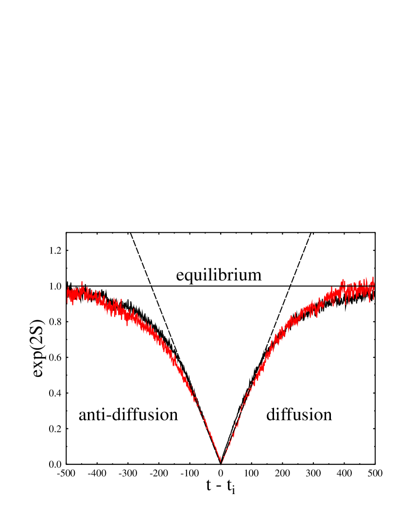
Figure 1: Boltzmann’s diffusive fluctuations in model (1.2) with parameter $C=15$: the square of phase space area occupied by $N$ independent trajectories (’particles’) vs. the time (number of map’s iterations $t-t_{i}$) counted off the instant $t_{i}$ of fluctuation maximum, or of minimal $\Gamma_{fl}$, for each of $N_{fl}$ superimposed BF separated by average period $P=\langle(t_{i}-t_{i-1})\rangle$. Straight lines show the expected dependence for anti–diffusion and diffusion (see text). Two slightly different curves correspond to $N=1$ (grey) and $N=4$ (black) with $\Gamma_{fl}=0.0001\ {\rm and}\ 0.1$; $N_{fl}=3352\ {\rm and}\ 2851$; $P=29863\ {\rm and}\ 35110$, respectively.

The data were obtained from running 4 and just 1 (!) trajectories for a sufficiently long time in order to collect fairly many BF which were superimposed in Fig.1 to clean up the regular BF from a ’podlike trash’ of stationary fluctuations. The size of BF chosen was approximately fixed by the condition that current $\Gamma(t)\leq\Gamma_{fl}$. In spite of inequality the mean values $\langle\Gamma(t_{i})\rangle=0.000033\ {\rm and}\ 0.069$ are close (in order of magnitude) to the fixed $\Gamma_{fl}$ values in Fig.1. Notice that for a slow diffusive kinetics the quantity $\exp{(2S)}\propto\sigma_{p}^{2}\propto\langle p^{2}\rangle$ while $\sigma_{x}$ remains constant.

The probability of BF can be characterized by the average period between them for which a very simple estimate

$$P\,\approx\,3\,\Gamma_{fl}^{-N}\,\approx\,3\,\exp{(-NS_{fl})}$$

is in a good agreement (upon including the empirical factor 3) with data in Fig.1.

In the example presented here the position of all BF in the phase space is fixed to $x_{fl}=1/2,\ p_{fl}=C/2$. If one lifts this restriction the probability of BF increases by a factor of $1/\Gamma_{fl}$, or by decrease of $N$ by one ($N\to N-1$), due to an arbitrary position of BF in phase space. In the former case, a chain of BF are but the well known Poincaré recurrences. What is less known that the latter are a particular and specific case of BF, and as such the recurrence of a trajectory in chaotic system is determined by the kinetics of the system. Recurrence of several $(N>1)$ trajectories can be also interpreted as the recurrence of a single trajectory in $N$ uncoupled freedoms.

As is seen in Fig.1 the irregular deviations from a regular BF are rapidly decreasing with the entropy $S\to S_{fl}$. One may get the impression that near BF maximum the motion becomes regular, hence the term ’optimal fluctuational path’ [1]. In fact, the motion remains diffusive down to the dynamical scale which in model (1.2) is $|\Delta p|\sim 1$ independent of parameter $C$.

Big fluctuations are not only perfectly regular by themselves but also surprisingly stable against any perturbations, both regular and chaotic. Moreover, the perturbations do not need to be small. At first glance, it looks very strange in a chaotic, highly unstable, dynamics. The resolution of this apparent paradox is in that the dynamical instability of motion does affect the BF instant of time $t_{i}$ only. As to the BF shape, it is determined by the kinetics whatever its mechanism, from purely dynamical one, like in model (1.2), to a completely noisy (stochastic, cf. Fig.1 above and Fig.4 in [1]). As a matter of fact, the fundamental Kolmogorov theorem [4] is related just to the latter case but remains valid in a much more general situation. Surprising stability of BF is similar to the full (less known) property of robustness of the Anosov (strongly chaotic) systems [11] whose trajectories get only slightly deformed under a small perturbation (for discussion see [12]). From a different perspective this stability can be interpreted as a fundamental property of the ’macroscopic’ description of BF. In such a simple few–freedom system like (1.2) the ’macroscopic’ refers to averaged quantities as $\sigma\,,\ \Gamma\,,\ S$, and the like. Still, a somewhat confusing result is in that the ’macroscopic’ stability comprises not only the relaxation of BF but also its rise as the both parts of BF appear always together. It may lead to another misunderstanding that the probability of fluctuation and relaxation are equal which is certainly wrong. The point is that the ratio of both (unequal!) probabilities is determined by a crossover parameter

$$R_{cro}(S_{fl})\,=\,\frac{P}{t_{r}}\,\approx\,\frac{3\,\exp{(-NS_{fl})}}{C^{2}}\,\gg\,1$$

Here the latter expression refers to model (1.2), and the inequality determines the region of BF where the time of awaiting BF is much longer than that of its immediate relaxation from a nonequilibrium ’macroscopic’ state (for further discussion see Section 6 below).

2 A new class of dynamical models:
What they are for?

A fairly simple picture of BF in the systems with equilibrium steady state (ES) is well understood by now, though not yet well known. To Boltzmann such a picture was the basis of his fluctuation hypothesis for our Universe. Again, as is well understood by now such a hypothesis is completely incompatible with the present structure of the Universe as it would immediately imply the notorious ’heat death’ (see, e.g., [13]). For this reason, one may even term such systems the heat death models. Nevertheless, they can be and actually are widely used in the description and study of local statistical processes in thermodynamically closed systems. The latter term means the absence of any heat exchange with the environment. Notice, however, that under conditions of the exponential instability of motion the only dynamically closed system is the whole Universe. Particularly, this excludes the hypothetical ’velocity reversal’ still popular in debates over ’irreversibility’ since Loschmidt (for discussion see, e.g., [12, 14] and Section 6 below).

In any event, dynamical models with ES do not tell us the whole story of either the Universe or even a typical macroscopic process therein. The principal solution of this problem, unknown to Boltzmann, is quite clear by now, namely, the ’equilibriumfree’ models are wanted. Various classes of such models are intensively studied today. Moreover, the celebrated cosmic microwave background tells us that our Universe was born already in the state of a heat death which, however, fortunately to us all became unstable due to the well–known Jeans gravitational instability [15]. This resulted in developing of a rich variety of collective processes, or synergetics, the term recently introduced or, better to say, put in use by Haken [16]. The most important peculiarity of such a collective instability is in that the total overall relaxation (to somewhere ?) with ever increasing total entropy is accompanied by an also increasing phase space inhomogeneity of the system, particularly in temperature. In other words, the whole system as well as its local parts become more and more nonequilibrium to the extent of the birth of a secondary dynamics which may be, and is sometime, as perfect as, for example, the celestial mechanics (for general discussion see, e.g., [17, 18, 12]).

I stress that all these inhomogeneous nonequilibrium structures are not BF like in ES systems but are a result of regular collective instability, so that they are immediately formed under a certain condition. Besides, they are typically dissipative structures in Prigogine’s term [19] due to exchange of energy and entropy with the infinite environment. The latter is the most important feature of such processes, and at the same time the main difficulty in studying the dynamics of those models both theoretically and in numerical experiments which are so much simpler for the ES systems. Usually, the investigations in this field are based upon statistical laws omitting the underlying dynamics from the beginning.

Recently, however, a new class of dynamical models has been developed by Evans, Hoover, Morriss, Nosé, and others [20, 21]. Some researchers still hope that such brand–new models will help to resolve the ’paradox of irreversibility’. A more serious reason for studying these models is in that they allow for a fairly simple inclusion in a few–freedom model the infinitely dimensional ’thermostat’, or ’heat bath’. This greatly facilitates both numerical experiments as well as the theoretical analysis. Particularly, by using such a model the derivation of Ohm’s law was presented in [22], thus solving ’one of the outstanding problems of modern physics’ [23] (for this peculiar dynamical model only!). The authors [22] claim that ”At present, no general statistical mechanical theory can predict which microscopic dynamics will yield such transport laws…” In my opinion, it would be more correct to inquire which of many relevant models could be treated theoretically, and especially in a rigorous way as was actually done in [22].

The zest of new models is the so–called Gauss thermostat, or heat bath (GHB). In the simplest case the motion equations of a particle in such a bath are [20, 21, 22]:

$$\frac{d{\bf p}}{dt}\,=\,{\bf F}\,-\,\zeta{\bf p}\,,\qquad\zeta\,=\,\frac{{\bf F}\cdot{\bf p}}{p^{2}}$$

where ${\bf F}$ is a given external force, and $\zeta$ stands for the ’friction coefficient’. The first peculiarity of such a ’friction’ is in its explicit time reversibility contrary to the ’standard friction’. The price for reversibility is the strict connection between the two forces, the friction and the external force ${\bf F}$. Moreover, and this is most important, the connection is such that $|{\bf p}|^{2}=p_{0}^{2}=const$ is the exact motion invariant:

$$\frac{d}{dt}\,\frac{|{\bf p}|^{2}}{2}\,=\,{\bf p}\cdot\frac{d{\bf p}}{dt}\,=\,{\bf p}\cdot{\bf F}\,-\,{\bf F}\cdot{\bf p}$$

The first of two identical terms represents the mechanical work of the external regular force ${\bf F}$, the spring of the external energy, while the second one describes the sink of energy into GHB. Thus, asymptotically as $t\to\infty$ the model describes a steady state only. This is the main restriction of such models. The particle itself does only immediately transfer the energy without any change of its own one due to the above constraint $|{\bf p}|^{2}=const$. In one freedom the latter would lead to a trivial solution $p=const$. So, at least two freedoms are required to allow for a variation of vector ${\bf p}$ in spite of constraint. For many interacting particles the constraint $\sum|{\bf p}_{i}|^{2}=const$ would be still less, hence reference to the Gauss ’Principle of Least Constraint’ [24] for deriving the reversible friction in Eq.(2.1). In the present paper the simplest case of $N$ noniteracting two–freedom particles is considered only as in [22].

The next important point is a special form of the energy in GHB which is the heat. In true heat bath it would be a chaotic motion of infinitely many particles therein. This is not the case in GHB, and one needs an additional force in Eq.(2.1) which would make the particle motion chaotic maintaining, at the same time, the constraint. Whether such an external to GHB chaos is equivalent to the chaos inside the true heat bath, at least statistically, remains an open question but it seems plausible from the physical viewpoint [22] (see also Ref.[25]). If so, the model describes the direct conversion of mechanical work into heat $Q$, and hence the permanent entropy production. The calculation of the later is not a trivial question (for discussion see [20, 21, 22]). In my opinion, the simplest way is to use the thermodynamic relation:

$$\frac{dS}{dt}\,=\,\frac{1}{T}\cdot\frac{dQ}{dt}\,,\qquad\frac{dQ}{dt}\,=\,{\bf p}\cdot{\bf F}$$

where $T=p_{0}^{2}$ is an effective temperature [22]. Since the input energy is of zero entropy (formal temperature $T_{in}=\infty$) the relation (2.3) determines the entropy production in the whole system (particles + GHB). Notice that in Eq.(2.3), as well as throughout this paper, the entropy $S$ is understood as determined in the standard way via a coarse–grained phase–space density (distribution function).

Meanwhile, usual interpretation of GHB models is quite different [20, 21, 22]. Namely, the entropy production (2.3) is expressed via the Lyapunov exponents $\lambda_{i}$ of particle’s motion:

$$\frac{dS}{dt}\,\equiv\,\frac{dS_{GHB}}{dt}\,\equiv\,-\frac{dS_{p}}{dt}\,=\,-\sum_{i}\,\lambda_{i}$$

where $S_{GHB}$ and $S_{p}$ is the entropy of GHB and of the ensemble of particles, respectively. An unpleasant feature of this relation is in that the latter equality holds true for the Gibbs entropy only which is conserved in Hamiltonian system modeled by the GHB. As a result the entropy of the total system (particles + GHB) remains constant (the second equality in Eq.(2.4)) which literally means no entropy production at all! Even though such an interpretation can be formally justified it seems to me physically misleading. In my opinion, the application of Lyapunov exponents would be better restricted to characterization of the phase–space fractal microstructure of particle’s motion (which is really interesting) retaining the universal coarse–grained definition of the entropy (cf. ES models in Section 1).

As was already mentioned above the GHB models describe the nonequilibrium steady states only. Moreover, any collective processes of interacting particles are also excluded, just those responsible for the very existence of regular nonequilibrium processes, particularly, of the field ${\bf F}$ in model (2.1). In a more complicated Nosé - Hoover version of GHB models these severe restrictions can be partly, but not completely, lifted. Whether it would be sufficient for the inclusion of collective processes remains, to my knowledge, an open question.

In any event, even the simplest GHB model like (2.1) represents a qualitatively different type of statistical behavior as compared to that in the ES models. The origin of this principal difference is twofold: (i) the external ’inexhaustible’ spring of energy, if only introduced ’by hand’, and (ii) a heat sink of infinite capacity which excludes any equilibrium.

In conclusion of this Section I formulate precisely the model to be considered below, in the main part of the paper. Choosing the model for numerical experiments I follow my favored ’golden rule’: construct the model as simple as possible but not simpler. In the problem under consideration the models studied already are mainly based on a well–known and well–studied ’Lorentz gas’ that is a particle (or many particles) moving through a set of fixed scatterers. A new element is a constant field accelerating particles. Actually, the Lorentz model becomes in this way the famous Galton Board [26], the very first model of chaotic motion, which had been invented by Galton for another purpose, and which has not been studied in detail until recently [20, 21, 22]. My model is still simpler, and is specified by the two maps: (i) the 2D Arnold cat map (1.1) to chaotize particles, and (ii) 1D–map version of Eq.(2.1):

$$\overline{p_{1}}\,=\,p_{1}\,+\,F\,-\,4Fp_{1}^{2}$$

where $p_{1}=p-p_{0}$, and parameter in Eq.(2.1) $p_{0}=1/2$. For $|F|<1/4$ the momentum $p$ remains within the unit interval ($0\leq p<1$) as in map (1.1). The principal relation (2.3) for the entropy reduces now also to the additional 1D map:

$$\overline{S}\,=\,S\,+(p_{1}\,+\,F)^{2}\,-\,p_{1}^{2}\,=\,S\,+\,2p_{1}F\,+\,F^{2}$$

where the entropy unit is changed by a factor of 2 for simplicity. Since $S$ is the entropy produced in GHB the latter map implicitly includes also the motion in the second freedom for each of noninteracting particles due to the Gauss constraint which guarantes the immediate transfer of energy to GHB.

In numerical experiments considered below an arbitrary number $N$ of noninteracting particles (trajectories) with random initial conditions were used. In this case, the Gauss constraint remained unchanged, and all trajectories were run simultaneously.

3 Nonmonotonic entropy production:
Local fluctuations

Statistical properties of the entropy growth in the model chosen are determined by the two first moments of the $p_{1}$ distribution function. In the limit $t\to\infty$ and/or $N\to\infty$ they are (per iteration and per trajectory):

$$\langle p_{1}\rangle\,=\,0\,,\qquad\langle p_{1}^{2}\rangle\,=\,\frac{1}{12}$$

where averaging is done over both the motion time $t$ (now the number of map’s iterations), and $N$ noninteracting particles (particle’s trajectories). In combination with Eq.(2.6) the first moment in Eq.(3.1) implies the linear growth of the average entropy (per trajectory):

$$\langle S(t)\rangle\,=\,t\,F^{2}$$

In this Section the statistics of local fluctuations is considered. A similar problem was studied in [27] for a more realistic model with many interacting particles. In the present model the local fluctuation is defined as follows. The total motion time $t_{f}$ is subdivided into many segments of equal duration $t_{1}$. On each segment $i=1,...,t_{f}/t_{1}$ the total change of entropy $S_{i}$ for all $N$ trajectories is calculated using Eq.(2.6) and represented as a dimensionless random variable

$$S_{\sigma}\,=\,\frac{S_{i}\,-\,\langle S_{i}\rangle}{\sigma}\,=\,\frac{S_{i}\,-\,\tau}{\sigma}$$

where $\langle S_{i}\rangle=Nt_{1}F^{2}=\tau$ (see Eq.(3.2)), and the rms fluctuation $\sigma$ is given by a simple relation (see Eqs.(2.6) and (3.1)):

$$\sigma^{2}\,=\,\frac{\tau}{3}$$

This relation neglects all the correlations which implies the standard Gaussian distribution:

$$G(S_{\sigma})\,=\,\frac{\exp{\left(-\frac{S_{\sigma}^{2}}{2}\right)}}{\sqrt{2\pi}}$$

An example of actual distribution function is shown in Fig.2 for a single trajectory with segment length $t_{1}=10,\,25,\,100$ iterations, and the number of segments up to $10^{7}$. A cap of the distribution is close to the standard Gauss (3.5) (see also Fig.3) but both tails clearly show a considerable enhancement of fluctuations depending on both $t_{1}$ and $N$ (in other examples, see below).

Figure 2: Distribution function $f(S_{\sigma})$ of local fluctuations in nonequilibrium steady state with $F=0.01$. Dashed line is standard Gauss (3.5); points represent the results of numerical experiments with $N=1$, and $t_{1}=10,\,25,\,100$

The shape of the tails is also Gaussian but the width is the larger the smaller $t_{1}$ and $N$. This is especially clear in a different representation of the data in Fig.3 where the ratio of empirical distribution to standard Gauss is plotted as a function of Gaussian variable $S_{G}=S_{\sigma}^{2}/2$.

Figure 3: The ratio of distribution $f(S_{\sigma})$ to the standard Gauss (3.5) (broken lines). The values of parameter $N/t_{1}$ from top to bottom are: 1/5 ($S_{\sigma}^{2}/2<7.5$, see text); 1/10; 1/100; 10/10, and 100/1. The oblique dotted straight line demonstrates the Gaussian shape of the tails.

Each run with particular values of $N$ and $t_{1}$ is represented by the two slightly different lines for both signs of $S_{\sigma}$. Besides fluctuations the difference apparently includes some asymmetry of the distribution with respect to $S_{\sigma}=0$. The origin of this asymmetry is not completely clear as yet. A sharp crossover between the two Gaussian distributions at $S_{G}\approx 3$ is nearly independent of the parameters $N$ and $t_{1}$ as is the top distribution below crossover. To the contrary, the tail distribution essentially depends on both parameters in a rather complicated way. The origin of the difference between the two Gaussian distributions apparently lies in dynamical correlations. In spite of a fast decay (see Section 1) the correlation in Arnold map (1.1) does affect somehow the big entropy fluctuations except the limiting case $N\gg t_{1}$ (two lower lines in Fig.3) when correlations vanish because of random and statistically independent initial conditions of many trajectories.

For any fixed parameters $N$ and $t_{1}$ the fluctuations are bounded ($F\ll 1$):

$$|S_{\sigma}|\,<\,\sqrt{3Nt_{1}}$$

which follows from Eqs.(2.6), (3.3), and (3.4). This is clearly seen in Fig.3 for minimal $Nt_{1}=5$. If instead only force $F$ is fixed, the relative entropy fluctuations

$$\frac{S_{i}}{\langle S_{i}\rangle}\,\approx\,\pm\,\frac{1}{F}$$

are also restricted but can be arbitrarily large for small $F$ and, moreover, of both signs. This implies a nonmonotonic growth of entropy at the expense of the segments with $S_{i}<0$.

The probability (in the number of trajectory segments) of extremely large fluctuations, Eqs.(3.6) and (3.7), is exponentially small (see Eq.(3.5) and below). However, the probability of the fluctuations with negative entropy change ($S_{i}<0$) (without time reversal!) is generally not small at all, reaching 50% as $\tau\to 0$ (for arbitrary $N$ and $t_{1}$). In principle, it is known, at least for the systems with equilibrium steady state (Section 1). Nevertheless, the first, to my knowledge, direct observation of this phenomenon in a nonequilibrium steady state [27] has so much staggered the authors that they even entitled the paper ’Probability of Second Law violations in shearing steady state’. In fact, this is simply a sort of peculiar fluctuations, big ones not so much with respect of their size but primarily of their probability (cf. discussion in Section 1). However, the important point is that all those negative entropy fluctuations (transforming the heat into work) are randomly scattered among the others of positive entropy, and for making any use of the former a Maxwell’s demon is required who is known by now to be well in a ’peaceful coexistence’ with the Second Law.

Another interesting limit is $t_{1}\to t_{f}\to\infty$ (a single segment) [27] while $\tau\to 0$ which is possible if $F\to 0$ too. In this case the probability of zero entropy change in the whole motion is also approaches 50%. However, the probability of any negative entropy fluctuation vanishes (see Eq.(3.3)). An interesting question is whether there exists some intermediate region of parameters where the latter probability would remain finite. In other words, are the Poincaré recurrences to negative entropy change $S_{i}<0$ possible in a nonequilibrium steady state as they are in the equilibrium (Section 1)? The answer to this question is given by the statistics of the global fluctuations.

4 Nonmonotonic entropy production:
Global fluctuations

The definition of the global fluctuations is similar to, yet essentially different from, that of the local fluctuations in the previous Section. Namely (cf. Eqs.(3.3) and (3.4)), the principal dimensionless random variable $S_{\sigma}(t)$ now explicitly depends on time:

$$S_{\sigma}(t)\,=\,\frac{S(t)\,-\,\langle S(t)\rangle}{\sigma}\,=\,\frac{S(t)\,-\,\tau}{\sigma}$$

where $S(t)$ is calculated from Eq.(2.6), $S(0)=0$, $\langle S(t)\rangle=NtF^{2}\equiv\tau$ (see Eq.(3.2)), and the rms fluctuation $\sigma$ is given by the same relation (3.4) with a new time variable $\tau$:

$$\sigma^{2}\,=\,\frac{\tau}{3}$$

In other words, the global fluctuations are described as a diffusion with the constant rate:

$$D\,=\,\frac{\sigma^{2}}{\tau}\,=\,\frac{1}{3}$$

Also, one can view the global fluctuations as a continuous time–dependent deviation of the entropy from its average growth unlike the local fluctuations in the ensemble of fixed trajectory segments (Section 3). Now, the primary goal is to find out if the entropy can reach the negative values $S(t)<0$ for $t\to\infty$. As was discussed in the previous Section this is possible at some finite segments of trajectory with the probability rapidly decreasing (but always finite) as the segment length grows.

In Fig.4 the three examples of global fluctuations are shown in a slightly different representation (cf. Eq.(4.1))

$$S_{g}(\tau)\,=\,\frac{S(\tau)}{\tau}\,-\,1$$

in order to always keep before one’s eyes the most important border $S(\tau)=0$ ($S_{g}(\tau)=-1$, a horizontal line in Fig.4).

Figure 4: Time dependence of the reduced global fluctuations $S_{g}(\tau)$, Eq.(4.4): three sets by $N=10$ trajectories with different initial conditions but the same initial entropy $S(0)=0$ and $F=0.01$. Horizontal solid line $S_{g}=0$ represents the average entropy growth. The lower solid line $S=0$ is the border between positive and negative entropy. A pair of dashed curves corresponds to the standard rms fluctuation $\sigma$, Eq.(4.2), and two solid curves represent the maximal diffusion fluctuations $\sigma_{b}$, Eq.(4.5).

Eventually, all trajectories converge to the average entropy growth (a horizontal line $S_{g}=0$ in Fig.4). During the initial stage of diffusion the probability of negative entropy is roughly 50%, similar to the local fluctuations (Section 3). However, at $\tau\raisebox{-2.15277pt}{\mbox{$\,\stackrel{{\scriptstyle>}}{{\sim}}\,$}}1$ the situation cardinally changes, so that all the trajectories move away from the border $S=0$. Moreover, the relative distance to the border with respect to the fluctuation size indefinitely increases.

The fluctuation size is characterized by the two parameters. The first one is the well known rms dispersion $\sigma$, Eq.(4.2) (two dashed curves in Fig.4), which estimates the fluctuation distribution width. In the problem under consideration the most important is the second characteristic, $\sigma_{b}$ (two solid curves in Fig.4), which sets the maximal size (the upper bound) of the diffusion fluctuations, and thus insures against the recurrence into the region $S<0$ in a sufficiently long time. The ratio of two sizes

$$R_{\sigma}(\tau)\,=\,\frac{\sigma_{b}}{\sigma}\,=\,\sqrt{2\ln{\ln{(A\tau)}}}$$

is given by the famous Khinchin law of iterated logarithm [28].

I emphasize again that the principal peculiarity and importance of border $\sigma_{b}$ is in that it characterizes a sharp drop of the fluctuation probability down to zero (in the limit $\tau\to\infty$). In other words, almost any trajectory approaches infinitely many times arbitrarily close to this border from below but the number of crossings the border remains finite. In Fig.4 this corresponds to the eternal confinement of trajectories in the gap between the two solid curves.

Such a surprising behavior of random trajectories is well known to mathematicians but, apparently, not to physicists. In Fig.5 a few examples of the fluctuation distributions are shown for illustration of that unpenetrable border.

Figure 5: Histogram of the global fluctuations in the number of entries per bin of width 0.02: $F=0.01;\ N=100;\ R_{\sigma}\approx 3$. From bottom to top in the leftmost part of figure: $\tau=10^{5}$ (dashed line); $10^{6}$ (two solid lines, different initial conditions); $10^{7}$ (circles); the total motion time $t=100\,\tau$ iterations. For comparison, the smooth dashed line shows unbounded Gaussian distribution (4.7) for $\tau=10^{6}$.

In Khinchin’s theorem a factor $A$ in Eq.(4.5) is irrelevant and set to $A=1$. This is because the theorem can be proved in the formal limit $\tau\to\infty$ only as most of theorems in the probability theory (as well as in the ergodic theory, by the way). However, in numerical experiments on a finite time, even if arbitrarily large, one needs a correction to the limit expression. Besides, it would be desirable to look at the border over the whole motion down to the dynamical time scale which is determined by the correlation decay. In the model under consideration it is of the order of relaxation time $t_{r}\sim 1$ (see Section 1). The additional parameter $A$ can be fixed by the condition

$$\sigma_{b}(\tau_{1})\,=\,\sigma(\tau_{1})\,,\qquad\tau_{1}\,=\,NF^{2}$$

for minimal $t=1$ on the dynamical time scale of the diffusion. Then, Eq.(4.5) implies $A\tau_{1}=5.2$ which is used in Figs.4 and 5. The condition assumed is, of course, somewhat arbitrary but the dependence on $A$ remains extremely weak provided $\tau_{1}\ll 1$.

The histogram in Fig.5 is given in the absolute numbers of trajectory entries into bins in order to graphically demonstrate a negligible number of exceptional crossings of the border. The exact formulation of Khinchin’s theorem admits a finite number of crossings in infinite time. Actually, all those ’exceptions’ are concentrated within a relatively short initial time interval $\tau\sim 1$ (for the accepted $A$ value, see Fig.4).

The distribution of entropy fluctuations between the borders is characterized by its own big fluctuations due to a large time interval ($\sim\tau$) required for crossing the distribution region (see Eq.(4.3)). The spectacular precipice of many orders of magnitude is reminiscent of a diffusion ’shock wave’ cutting away the Gaussian tail. Unbounded Gauss is also shown in Fig.5 by the smooth dashed line.

In variable $S_{\sigma_{b}}=S_{\sigma}/R_{\sigma}$ the standard Gauss is no longer a stationary distribution (cf. Eq.(3.5)):

$$\sqrt{2\pi}\,G(S_{\sigma_{b}})\,=\,R_{\sigma}(\tau)\cdot\exp{\left(-\frac{S_{\sigma_{b}}^{2}}{2}R_{\sigma}^{2}(\tau)\right)}$$

Both the probability density at the border $|S_{\sigma_{b}}|=1$ as well as the integral probability beyond that are slowly decreasing $\sim 1/\ln{(A\tau)}$. The ’shock wave’ decays but still continues to ’hold back’ the trajectories.

Thus, unlike unrestricted entropy fluctuations out of the equilibrium steady state (Section 1) the strictly restricted fluctuations in the nonequilibrium steady state get well separated, in a short time, from the region of negative entropy, separated in a large excess which keeps growing in time. In other words, the Poincaré recurrences to any negative entropy quickly and completely disappear leaving the system with ever increasing, even if nonmonotonically, entropy.

As nonequlibrium steady state involves a heat bath of infinite phase space volume (or its nice substitute, the Gauss heat bath), the Poincaré recurrence theorem is not applicable. Yet, the ’anti–recurrence’ theorem is not generally true either. For example, the entropy repeatedly crosses the line $S=\tau$ of the average growth in spite of infinite heat bath, yet it does not so for the line $S=0$ of the initial entropy.

5 Big entropy fluctuations in critical dynamics

The strict restriction of the global entropy fluctuations in a nonequilibrium steady state considered in the previous Section is a result of the ’normal’, Gaussian, diffusion of the entropy with a constant rate (4.3), and with the surprising unpenetrable border (4.5). In turn, this is related to a particular underlying dynamics of the model (1.1) with very strong statistical properties. Notice that the border (4.5) is of a statistical nature as it is much less than the maximal dynamical fluctuation (3.7).

However, it is well known by now that, generally, the homogeneous diffusion can be ’abnormal’ in the sense that the diffusion rate does depend on time:

$$D(t)\,\sim\,t^{c_{D}}\,,\qquad-1\,\leq c_{D}\,\leq 1$$

where $c_{D}$ is the so–called critical diffusion exponent. The term ’critical’ refers to a particular class of such systems with a very intricate and specific structure of the phase space (see, e.g., [29] and references therein). The ’normal’ diffusion corresponds to $c_{D}=0$ while a positive $c_{D}>0$ represents a superfast diffusion with the upper bound $c_{D}=+1$, the maximal diffusion rate possible for a homogeneous diffusion. The latter is, of course, most interesting case for the problem under consideration here. A superslow diffusion for a negative $c_{D}<0$ is also possible with the limit $c_{D}=-1$ which means the absence of any diffusion for $c_{D}<-1$. An interesting example of a superslow diffusion with $c_{D}=-1/2$ was considered in [30]. Besides a particular application to the plasma confinement in magnetic field the example is of a special interest as this slow diffusion is a result of the time–reversible diffusion of particles in a chaotic magnetic field. For other examples and various discussions of abnormal diffusion see [31].

A number of dynamical models exhibiting the superfast diffusion are known including the limiting case $c_{D}=1$ [29, 32]. Interestingly, a simple simulation of abnormal diffusion is possible by a minor modification of the model under consideration. It concerns the additional 1D map (2.6) only which now becomes:

$$\overline{S}\,=\,S\,+(\,2p_{1}F\,+\,F^{2})\cdot t_{s}$$

Here the new variable $t_{s}$ is defined also by a simple relation:

$$t_{s}\,=\,s^{-c_{s}}\,,\qquad s=1\,-\,2|p_{1}|$$

where $s$ is the distance from any of the two borders $p_{1}=\pm 0.5$ homogeneously distributed within the interval ($0<s<1$). The quantity $t_{s}>1$ describes the sticking of a trajectory in the ’critical structure’ concentrated near $s=0$. Actually, in the model there is no such a structure, yet the effect of that is simulated by the ’sticking time’ $t_{s}$ which enhances both the fluctuations and the average entropy (5.2). In a sense, such a simulation is similar, in spirit, to that of the Gauss heat bath. All the properties of that sticking are described by a single parameter $c_{s}$, the critical sticking exponent ($0\leq c_{s}\leq 1$). Particularly, it is directly related to the diffusion exponent $c_{D}$ (see below).

The statistical properties of abnormal diffusion in this model are determined by the two first moments of $t_{s}$ distribution which are directly evaluated from the above relations as follows. For the first moment it is

$$\langle t_{s}\rangle\,=\,\int_{0}^{1}t_{s}(s)\,ds\,=\,\frac{1}{1\,-\,c_{s}}\,,\qquad c_{s}\,<\,1$$

and

$$\langle t_{s}\rangle\,\approx\,\ln{\frac{1}{s_{1}}}\,\approx\,\ln{t}\,,\qquad c_{s}\,=\,1$$

In the latter case the integral diverges, and is determined by the minimal $s\approx s_{1}\sim 1/t$ reached over time $t$ which is the total motion time in map’s iterations. This should be distinguished from the ’physical time’ in a true model of the critical structure

$$\widetilde{t}\,\approx\,t\cdot\langle t_{s}\rangle\,\approx\,\left\{\begin{array}[]{ll}\frac{t}{1\,-\,c_{s}}\,,&c_{s}\,<\,1\\ t\,\ln{t}\,,&c_{s}\,=\,1\end{array}\right.$$

In a similar way the second moment is given by three relations:

$$\langle t_{s}^{2}\rangle\,=\,\frac{1}{1\,-\,2c_{s}}\,,\qquad c_{s}\,<\,\frac{1}{2}$$

for the normal diffusion,

$$\langle t_{s}^{2}\rangle\,\approx\,\ln{\frac{1}{s_{1}}}\,\approx\,\ln{t}\,,\qquad c_{s}\,=\,\frac{1}{2}$$

in the critical case, and

$$\langle t_{s}^{2}\rangle\,\approx\,\frac{s_{1}^{1-2c_{s}}}{2c_{s}\,-\,1}\,\approx\,\frac{t^{2c_{s}-1}}{2c_{s}\,-\,1}\,,\qquad\frac{1}{2}\,<\,c_{s}\,\leq\,1$$

for the superfast diffusion.

The average entropy production is found from Eq.(5.2):

$$\langle S_{i}\rangle\,=\,NF^{2}t\langle t_{s}\rangle\,=\,NF^{2}\widetilde{t}\,\equiv\,\tau$$

with redefined time variable $\tau$ (cf. Eq.(3.3)). In this Section the simplest case of a single trajectory ($N=1$) will be considered only.

Evaluating the superfast diffusion requires a slightly different averaging $\langle(2p_{1}t_{s})^{2}\rangle$ (see Eq.(5.2)). Yet it is easily verified that asymptotically, as $\tau\to\infty$, the difference with respect to Eq.(5.6c) vanishes, and one arrives at the following estimate for the critical rms dispersion $\sigma_{cr}$:

$$\frac{\sigma_{cr}^{2}(\tau)}{B^{2}}\,=\,\widetilde{t}D(\widetilde{t})\,=\,F^{2}\langle t_{s}^{2}\rangle t\,=\,\frac{(1\,-\,c_{s})^{2c_{s}}}{2c_{s}\,-\,1}\cdot\frac{\tau^{2c_{s}}}{F^{4c_{s}-2}}$$

if $1/2<c_{s}<1$ (5.6c), and

$$\frac{\sigma_{cr}(\tau)}{B}\,=\,\frac{\tau}{F\cdot\ln{(\tau/F^{2})}}$$

in the most interesting limiting case $c_{s}=1$. Here empirical factor $B\sim 1$ accounts for all the approximations in the above relations.

The limit $c_{s}\to 1$ in Eq.(5.8a) crucially differs from the limiting relation (5.8b). The origin of this discrepancy is Eq.(5.4a). A more accurate evaluation for $c_{s}\approx 1$ reads:

$$\langle t_{s}\rangle\,=\,\int_{s_{1}}^{1}t_{s}(s)\,ds\,=\,\frac{1\,-\,s_{1}^{1-c_{s}}}{1\,-\,c_{s}}\,=\,\frac{1\,-\,\exp{[(1-c_{s})\ln{s_{1}}]}}{1\,-\,c_{s}}$$

where $s_{1}\sim 1/t$ is the minimal $s$ over $t$ map’s iterations (cf. Eq.(5.4b)). Hence, the relation (5.4a) is valid under condition $\epsilon\ln{t}>1$ only ($\epsilon=1-c_{s}$) while in the opposite limit $\langle t_{s}\rangle\approx\ln{t}$ as for $c_{s}=1$, Eq.(5.4b). The crossover between the two scalings is at

$$t_{cro}\,\sim\,{\rm e}^{1/\epsilon}\,,\qquad\tau_{cro}\,\sim\,\frac{{\rm e}^{1/\epsilon}}{\epsilon}\,F^{2}$$

The deviation from Eq.(5.8a) is essential for a sufficiently small $\epsilon$ only.

The ratio of fluctuations to the average entropy production is given by the reduced entropy (see Eq.(4.4))

$$S_{g}=\pm\frac{\sigma_{cr}}{\tau}\,\approx\,\pm\frac{B}{F\cdot\ln{(\tau/F^{2})}}$$

where the latter expression is estimate (5.8b) for the rms fluctuations. They are slowly decreasing with time, and at $\tau\raisebox{-2.15277pt}{\mbox{$\,\stackrel{{\scriptstyle>}}{{\sim}}\,$}}\tau_{0}=F^{2}\exp{(1/F)}$ the rms line crosses the border $S_{g}=-1$ of zero entropy. Afterwards, the entropy remains mainly positive. To be more correct, the probability for a trajectory to enter into the region of negative entropy is systematically decreasing with time, rather slow though. This is to be compared with the $F$–independent crossover $\tau_{0}=1/3$ and a rapid drop of the probability to return back to $S<0$ in case of the normal diffusion (Section 4).

However, there exists another mechanism of big fluctuations, specific for the critical dynamics. Namely, a separated individual fluctuation can be produced as a result of a single extremely big sticking time $t_{s}$ over the total motion up to the moment the fluctuation springs up in a single map’s iteration. I remind that in the present model each sticking corresponds to just one map’s iteration. The increments of dynamical variables in such a jump are obtained from Eq.(5.2):

$$\Delta S\,=\,\pm Ft_{s}\,,\qquad\Delta\tau\,=\,F^{2}t_{s}$$

where $t_{s}\gg 1\ (2p_{1}\approx 1)$ is assumed (a big fluctuation). Then, the reduced fluctuation

$$S_{g}\,\approx\,\frac{S}{\tau}\,=\,\pm\frac{Ft_{s}}{\tau\,+\,F^{2}t_{s}}\,\approx\,\pm\frac{1/F}{1\,+\,\frac{\tau}{\Delta\tau}}$$

The maximal single sticking time over the motion time $t$ is, on the average

$$\langle t_{s}\rangle\,\approx\,t\,\ln{t}\,=\,\frac{\tau}{F^{2}}$$

Hence, a single fluctuation (5.13) has the upper bound

$$|S_{g}|\,\raisebox{-2.15277pt}{\mbox{$\,\stackrel{{\scriptstyle<}}{{\sim}}$\,}}\,\frac{A}{F}$$

Here an empirical factor $A\sim 1$ is introduced similar to Eq.(5.8b).

The border (5.15) considerably exceeds the rms diffusion fluctuation (5.11) and, what is even more important, the former never crosses the line of zero entropy $S_{g}=-1$. Thus, the critical fluctuations repeatedly bring the system into the region of negative entropy. This is because the upper bound (5.15) does not depend on time $\tau$ provided $\Delta\tau\raisebox{-2.15277pt}{\mbox{$\,\stackrel{{\scriptstyle>}}{{\sim}}\,$}}\tau$ in Eq.(5.13). However, in a chain of successive fluctuations the values of $\tau$ in Eqs.(5.13) and (5.14) are not generally equal. While in the former relation it is always the total motion time as assumed above, in Eq.(5.14) it should be the preceeding period of fluctuations: $\tau_{n}\to P_{n}<\tau_{n}$ where $n$ is the serial number of fluctuations. Hence, the approach to the upper bound (5.15) is only possible under condition $P_{n}\gg P_{n-1}$ which implies $P_{n}\approx\tau_{n}$. Thus, the fluctuations become more and more rare with a period growing exponentially in time. In other words, the fluctuations are stationary in $\ln{\tau}$ with a quite big mean period $\langle\ln{P}\rangle\approx 5$ (see Fig.6).

In Fig.6 an example of a few big critical fluctuations in the limiting case $c_{s}=1$ is presented for five single fairly long trajectories with different initial conditions, and the motion time up to $\tau\approx 5\times 10^{9}$ and $t=10^{10}$ iterations. To achieve such a long time the force was decreased down to $F=0.1$ (see Eq.(5.14)).

Figure 6: Time dependence of 26 big fluctuations in critical dynamics: 5 single trajectories up to $10^{10}$ iterations, $c_{s}=1,\ F=0.1$. Only fluctuations with $F|S_{g}|>0.3$ are shown, each one by a pair of points connected by the straight line: the big fluctuation itself (stars), and that at the preceding map’s iteration (circles, see text). Two dashed curves show the rms fluctuations of $F|S_{g}|$, Eq.(5.11) with $B=1$. Horizontal dotted lines mark the upper bound, Eq.(5.15) with $A=1$.

Unlike a similar Fig.4 for the normal diffusion, only a few big fluctuations with $F|S_{g}|>0.3$ are presented in Fig.6. For a full picture of critical fluctuations the required output becomes formidably long. The distribution of all fluctuations, independent of time, is shown below in Fig.7.

Each fluctuation in Fig.6 is presented by a pair of $FS_{g}$ values connected by the straight line: one at map’s iteration just before the fluctuation (circles), and the other one (stars) at the next iteration when the fluctuation springs up (see above). Both are plotted at the same, latter, $\tau$ to follow the pairs. This somewhat shifts the circles to the right.

The most important, if only preliminary, result of numerical experiments is confirmation of the fluctuation upper bound (5.15) independent of time. As expected, the circles represent considerably smaller $F|S_{g}|$ values roughly following the diffusive scaling (5.11).

The border (5.15) qualitatively reminds the strict upper bound for the normal diffusion (Section 4), including a logarithmic ratio with respect to the rms size (4.5), as compared to the ratio

$$R_{cr}(\tau)\,\approx\,\ln{(\tau/F^{2})}$$

in the critical diffusion. An interesting question if the new, critical, border is also as strict as the old one in the normal diffusion remains, to my knowledge, open, at least for the physical model under consideration where the superdiffusion is caused by a strong long–term correlation of successive entropy changes due to the sticking of trajectory.

However, for a much simpler problem of statistically independent changes various generalizations of Khinchin’s theorem to the abnormal diffusion were proved by many mathematicians (see, e.g., [33]). In the present model it is just the case for the description in map’s time $t$ with statistically independent iterations. The most general and complete result has been recently obtained by Borovkov [34]. In the present notations it can be approximately represented in a very simple form for the ratio (5.16):

$$R_{cr}\,=\,{\sigma_{b}\over\sigma}\,\sim\,(\ln{t})^{c_{s}}\,\approx\,\ln{(\tau/F^{2})}$$

in the whole interval ($1/2<c_{s}\leq 1$) of the superdiffusion where the physical time $\tau$ is determined by Eq.(5.7). Then, for most important reduced fluctuation (5.13) one arrives at the two relations

$$|S_{g}|\,\raisebox{-2.15277pt}{\mbox{$\,\stackrel{{\scriptstyle<}}{{\sim}}$\,}}\,{\sigma_{b}\over\tau}\,\sim\,\frac{\tau^{c_{s}-1}}{F^{2c_{s}-1}}\cdot\left(\ln{{\tau\over F^{2}}}\right)^{c_{s}}$$

for $c_{s}<1$, and

$$|S_{g}|\,\raisebox{-2.15277pt}{\mbox{$\,\stackrel{{\scriptstyle<}}{{\sim}}$\,}}\,{\sigma_{b}\over\tau}\,\sim\,{1\over F}$$

in the limiting case $c_{s}=1$. The latter confirms estimate (5.15) above which, in turn, is in a good agreement with the empirical data in Fig.6. In any event, a simple physical estimate (5.15) seems to provide an efficient description of the fluctuation upper bound.

In Fig.7 an example of all (at each map’s iteration) fluctuations is shown for the data from the same runs as in Fig.6. Besides very large overall distribution

Figure 7: Histogram of critical fluctuations in the number of entries per bin of width 0.007 for the data in Fig.6. The border $S=0$ corresponds to $FS_{g}=-F=-0.1$. The points for the longest trajectory are connected by line.

fluctuations a sharp drop by about four orders of magnitude is clearly seen near the expected upper bound (5.15). It looks similar to the drop in Fig.5 for the normal diffusion.

Thus, the critical diffusion results in infinitely many recurrences far into the region of negative entropy $S<0$ (for $F\ll 1$), the sojourn time over there being comparable to the total motion time. Of course, the former is less than 50% on an average, so that asymptotically in time the entropy keeps always growing. In this respect, the global critical fluctuations are similar to the local ones in the normal diffusion (Section 3).

Notice, however, that the upper bound $\sigma_{b}/\tau\sim 1/F$ (5.18b) is permanent in the strict limit $c_{s}=1$ only. For any deviation from this limit $\epsilon=1-c_{s}>0$ this bound lasts a finite time determined by the crossover (5.10) ($\tau\raisebox{-2.15277pt}{\mbox{$\,\stackrel{{\scriptstyle<}}{{\sim}}$\,}}F^{2}\exp{(1/\epsilon)}/\epsilon$) to decreasing $\sigma_{b}/\tau\to 0$ (5.18a). Another interesting representation of such an intermediate behavior is the crossover in the sticking exponent:

$$\epsilon\,\raisebox{-2.15277pt}{\mbox{$\,\stackrel{{\scriptstyle<}}{{\sim}}$\,}}\,{1\over\ln{(\tau/F^{2})}}\,\approx\,F|S_{g}|$$

which is actually shown in Fig.6 by the upper dashed line. For the longest $\tau=5\times 10^{9}$ the latter crossover $\epsilon_{cro}\approx 0.037$.

6 Discussion and conclusion

In the present paper the results of extensive numerical experiments on big entropy fluctuations in a nonequilibrium steady state of classical dynamical systems are presented, and their peculiarities are analysed and discussed. For comparison, some similar results for the equilibrium steady state are briefly described in the Introduction (the latter will be published in detail elsewhere [10]).

All numerical experiments have been carried out on the basis of a very simple model - the Arnold cat map (1.1) on a unit torus - with only three minor, but important, modifications which allowed for comprising all the problems under consideration above. The modifications are:

(1) Expansion of the torus in $p$ direction (1.2) which allows for more impressive diffusive fluctuations out of the equilibrium steady state (Fig.1 in Section 1).

(2) Addition of a 1D map (2.5) with the constant driving force $F$, and with ingenious time–reversible friction force which represents the so–called Gauss heat bath, and which allows for modeling a physical thermostat of infinitely many freedoms [20, 21]. This modification is the principal one in the present studies of fluctuations in a nonequilibrium steady state (Sections 3 - 5).

(3) Addition of a new parameter $t_{s}$ (5.3) in map (5.2) which allows for the study of very unusual fluctuations of an ’abnormal’, critical, dynamical diffusion (Section 5).

Big fluctuations in an equilibrium steady state (ES) are briefly considered in Section 1. The simplest one of this class, which I call the Boltzmann fluctuation, is shown in Fig.1. It is obviously symmetric with respect to time reversal, so that at least in this case there is no physical reason at all for the conception of the notorious ’time arrow’. Nevertheless, a related conception, say, thermodynamic arrow, pointing in the direction of the average increase of entropy, makes sense in spite of the time symmetry. The point is that the relaxation time of the fluctuation is determined by model’s parameter $C$ only, and does not depend on the fluctuation itself. On the contrary, the expectation time for a given fluctuation, or the mean period between successive fluctuations, rapidly grows with the fluctuation size and with the number of trajectories (or freedoms).

Besides the simplest Boltzmann fluctuation, various others are also possible, typically with a much less probability. One of those - the two correlated Boltzmann fluctuations, which I call the Schulman fluctuation - was recently described in [36] using the same Arnold cat map. However, such a model has nothing to do with cosmology as was speculated in [36]. At least, the Universe we live in as well as most macroscopic phenomena therein require the qualitatively different models, ones without equilibrium steady state. Such structures do appear (with probability 1) as a result of certain regular collective processes which lead to very complicated nonequilibrium and inhomogeneous states with ever increasing entropy. This is in contrast with a constant, on an average, entropy in ES systems.

A nonequilibrium steady state, the main subject of the present studies, is but a little, characteristic though, piece of the chaotic collective processes. In the model (2.5) the driving force $F$ represents a result of some preceding collective processes, the spring of free energy, while the Gauss friction does so for an infinite environment around, the sink of the energy, converting the work into heat, on the average. An interesting peculiarity of such systems is in that the big fluctuations may do, and do indeed under certain conditions, the opposite, converting back some heat into the work.

Two types of fluctuations were studied:

(i) the local ones on a set of trajectory segments of length $t_{1}$ iterations and of entropy change $S_{i}$ (Section 3), and

(ii) ones of the global entropy $S(t)$ along a trajectory with respect to the initial entropy set to zero: $S(0)=0$ (Sections 4 and 5).

The former were found to have a stationary unrestricted distribution close to the standard Gauss with some enhancement of unknown mechanism for large fluctuations. The study of the latter effect will be continued. The distribution is symmetric with respect to the average entropy, growing in proportion to time in agreement with previous studies on a more complicated (and more realistic) model [27]. Even though the distribution is asymmetric with respect to zero entropy change, the probability of negative $S_{i}<0$ is generally not small provided $F^{2}\,Nt_{1}\raisebox{-2.15277pt}{\mbox{$\,\stackrel{{\scriptstyle<}}{{\sim}}$\,}}1$. This phenomenon, apparently a new one in the nonequilibrium steady state, was first observed in [27] but has been interpreted there as a violation of the Second Law. It seems to be the reflection of a common, but wrong in my opinion, understanding the Second Law as a monotonic growth of the entropy, thus neglecting all the fluctuations including the large ones. Meanwhile, the nonmonotonic rise of entropy is clearly seen, for instance, in Fig.4, and discussed in detail in Sections 3 and 4.

The behavior of the global entropy is completely different as the data in the same Fig.4 demonstrate (Section 4). Even though the entropy evolution remains nonmonotonic it quickly crosses the line of the initial zero entropy and does not return back into the region of negative entropy $S<0$. This is insured by the famous Khinchin theorem about the strict upper bound for the diffusion process. At least for physicists, such a limitation of statistical nature for a random motion is surprising and apparently less known. That unidirectional evolution is the most important distinction of the nonequilibrium steady states from the equilibrium ones.

This farther justifies the conception of the thermodynamic arrow pointing to a larger, on the everage, entropy. Yet, again it has nothing to do with the properties of time. Of course, upon formal time reversal the entropy will systematically decrease, also in the model under consideration because the Gauss heat bath is time reversible. Within the steady state approximarion, or rather restriction, this would be an infinitely large fluctuation which never came to the end. However, such a fluctuation would never occur either, as a result of the natural time evolution of the system, opposite to the case of equilibrium fluctuations. The ultimate origin of that crucial difference is in that the former process, even asymptotically in time, is a tiny little part of the full underlying dynamics of an infinite system. Particularly, the initial state $S(0)=0$ is not a result of the preceding fluctuation, as is the case in ES, but has been eventually caused, for instance, by instability of the initial ES at a very remote time in the past. If one would imagine the time reversal at that instant nothing were changed as the thermodynamic arrow does not depend on the direction of time provided, of course, the time reversible fundamental dynamics. That is just this universal overall dynamics which unifies the time for all the interacting objects like particles and fields throughout the Universe. Particularly, it is incompatible with the two opposite time arrows - an old Boltzmann’s hypothesis [2] - which still has some adherents [36].

Coming back to a particular phenomenon of nonequilibrium steady states it is worth to mention that the regularities of the fluctuations in those, both local and global, can be applied, at least qualitatively, to a small part of a big fluctuation in a statistical equilibrium (Fig.1) on both sides of the maximum. This interesting question will be considered in detail elsewhere [10].

Finally, some preliminary numerical experiments on the global entropy fluctuations and the theoretical analysis were carred out in a special case of the critical dynamics which turned out to be the most interesting one for the problem in question (Section 5). The point is that the critical dynamics leads to an ’abnormal’ superdiffusion with the rate $D\propto\tau^{2c_{s}-1}$ and rms fluctuation size $\sigma_{cr}\propto\tau^{c_{s}}$ where $c_{s}$ is a new parameter of the third model ($1/2<c_{s}\leq 1$). This implies the reduced entropy $|S_{g}|\propto\tau^{c_{s}-1}$ decreasing very slowly for $c_{s}\approx 1$ as compared to the normal diffusion $|S_{g}|\propto 1/\sqrt{\tau}$. In the limiting case $c_{s}=1$ the entropy $|S_{g}|\propto 1/\ln{\tau}$ is still decreasing. However, besides diffusive fluctuations there is a set of infinitely many separated fluctuations whose size does not decrease with time at all (Fig.6). In other words, these preliminary numerical experiments suggest that in the limiting case of the critical dynamics the Poincaré recurrences to the initial state $S=0$ and beyond keep to repeatedly occur without limit. These are preliminary results to be confirmed and farther studied in detail.

In the present studies the fluctuations in classical mechanics are presented only. Generally, the quantum fluctuations would be rather different. However, according to the Correspondence Principle, the dynamics and statistics of a quantum system in quasiclassics are close to the classical ones on the appropriate time scales of which the longest one corresponds just to the diffusive kinetics providing transition to the classical limit (for details see [12, 35]). Interestingly, the computer classical dynamics that is the simulation of a classical dynamical system on digital computer is of a qualitatively similar character. This is because any quantity in computer representation is discrete (’overquantized’). As a result the correspondence between the classical continuous dynamics and its computer representation in numerical experiments is restricted to certain finite time scales like in the quantum mechanics (see two first references [35]).

Discreteness of computer phase space leads to another peculiar phenomenon: generally, the computer dynamics is irreversible due to the rounding–off operation unless the special algorithm is used in numerical experiments. Nevertheless, this does not affect the statistical properties of chaotic computer dynamics. Particularly, the statistical laws in computer representation remain time–reversible in spite of (nondissipative) irreversibility of the underlying dynamics. This simple example demonstrates that, contrary to a common belief, the statistical reversibility is a more general property than the dynamical one.

In the very conclusion I would like to make a brief remark on a very difficult, complicated and vague problem - the so–called (physical) causality principle that is the time–ordering of the cause and effect. Discussion of this important problem in detail will be published elsewhere [37]. Here I mention, as an example, a simple Boltzmann’s fluctuation shown in Fig.1. I adhere to the idea of statistical nature of causality. Indeed, the cause is, by definition, an ’absolutely’ independent event which is only possible in the chaotic dynamics. Moreover, in any purely dynamical description the conception of cause loses its usual physical meaning. For example, the initial conditions do precisely determine the whole infinite trajectory ($-\infty<t<\infty$) that is both the future as well as the past of such a ’cause’. In case of a single Boltzmann’s fluctuation an appropriate cause would be the minimal entropy (at $t=t_{i}$ in Fig.1). This was exactly the procedure used in numerical experiments for the location of a fluctuation of an approximately given size. The principal difference from the exact dynamical initial conditions is in that the former cause is an approximate (e.g., average) fluctuation’s size which is quite sufficient for the complete statistical description of the fluctuation, yet does leave behind enough freedom for independence from other events like preceding fluctuations. However, this cause does determine not only the future relaxation of the fluctuation (in agreement with the causality principle) but also the past rise of the same fluctuation which is a violation of causality, or acausality (spontaneous rise of a fluctuation), or anti–causality which the latter is perhaps the most appropriate term. Upon the time reversal, the causality/anticausality exchange which allows for a conception of the causality arrow but, again, without any reference to the time of physics. In such a philosophy the directions of both arrows, thermodynamic and causal one, do coincide independent of the direction of time. An important point of this philosophy is in that the concept ’arrow’ is related to the interpretation of a physical phenomenon rather than to the phenomenon itself. Particularly, a question ’how to fix or maintain the arrow’ [36] is up to the researcher alone. In a more complicated Schulman’s double fluctuation the mechanism of causality becomes more interesting [36], and will be discussed, from a different point of view, in [37].

Acknowledgments. I am grateful to Wm. Hoover for attracting my attention to a new class of highly efficient dynamical models with the Gauss heat bath, and for stimulating discussions and suggestions. I very much appreciate the initial collaboration with O.V. Zhirov which, hopefully, will continue before long. I am indebted to A.A. Borovkov for elucidation of Khinchin’s theorem and of its recent generalizations to the ’abnormal’ superdiffusion.

References

- [1] D.G. Luchinsky, P. McKlintock and M.I. Dykman, Rep. Prog. Phys. 61, 889 (1998)
- [2] L. Boltzmann, Vorlesungen über Gastheorie, Leipzig, 1896/98 (English translation in: Lectures on gas theory, Univ. of California Press, 1964).
- [3] E. Schrödinger, Über die Umkehrung der Naturgesetze, Sitzungsber. Preuss. Akad. Wiss. (1931), 144.
- [4] A.N. Kolmogoroff, Math. Ann. 113, 766 (1937); see also ibid. 112, 155 (1936); Selected papers on probability theory and mathematical statistics, Nauka, Moscow, 1986, pp. 197 and 173 (in Russian).
- [5] A.M. Yaglom, Dokl. Akad. Nauk SSSR 56, 347 (1947); Mat. Sbornik 24, 457 (1949).
- [6] Proc. 20th IUPAP Intern. Conference on Statistical Physics (Paris, 1998), Physica A 263, # 1-4 (1999), p. 516.
- [7] I.P. Kornfeld, S.V. Fomin and Ya.G. Sinai, Ergodic Theory, Springer, 1982.
- [8] V.I. Arnold and A. Avez, Ergodic Problems of Classical Mechanics, Benjamin, 1968.
- [9] A. Lichtenberg and M. Lieberman, Regular and Chaotic Dynamics, Springer, 1992.
- [10] B.V. Chirikov and O.V. Zhirov, Large fluctuations in statistical equilibrium (in preparation).
- [11] D.V. Anosov, Dokl. Akad. Nauk SSSR 145, 707 (1962).
- [12] B.V. Chirikov, Natural Laws and Human Prediction, in: Law and Prediction in the Light of Chaos Research, Eds. P. Weingartner and G. Schurz, Springer, 1996, p. 10; Open Systems & Information Dynamics 4, 241 (1997).
- [13] L.D. Landau and E.M. Lifshitz, Course of Theoretical Physics, Vol. 5, Statistical Physics, Part 1, Pergamon Press, 1980.
- [14] B.V. Chirikov, Dynamische und statistische Gesetze in der klassischen Mechanik, Wiss. Zs. Humboldt Univ. zu Berlin, Ges.-Sprachw. R. 24, 215 (1975).
- [15] J. Jeans, Phil. Trans. Roy. Soc. A 199, 1 (1929).
- [16] H. Haken, Synergetics, Springer, 1978.
- [17] A. Turing, Phil. Trans. Roy. Soc. Lond. B 237, 37 (1952); G. Nicolis and I. Prigogine, Self–Organization in Nonequilibrium Systems, Wiley, 1977.
- [18] A. Cottrell, Emergent properties of complex systems, in: The Encyclopedia of Ignorance, Eds. R. Duncan and M. Weston-Smith, Pergamon Press, 1977, p.129.
- [19] P. Glansdorf and I. Prigogine, Thermodynamic theory of structure, stability, and fluctuations, 1971.
- [20] D. Evans and G. Morriss, Statistical mechanics of nonequilibrium liquids, Academic, 1990; Wm. Hoover, Computational statistical mechanics, Elsevier, 1991; Proc. Workshop on Time–Reversal Symmetry in Dynamical Systems (Warwick, 1996), Physica D 112, # 1-2 (1998).
- [21] Wm. Hoover, Time reversibility, computer simulation, and chaos, World Scientific, 1999.
- [22] N.I. Chernov, G. Eyink, J. Lebowitz and Ya.G. Sinai, Phys. Rev. Lett. 70, 2209 (1993).
- [23] R. Peierls, in: Theoretical Physics in Twentieth Century, Eds. M. Fiera and V. Weisskopf, Wiley, 1961.
- [24] K. Gauss, J. Reine Angew. Math. IV, 232 (1829).
- [25] Wm. Hoover, Phys. Lett. A 255, 37 (1999).
- [26] F. Galton, Natural inheritance, London, 1889.
- [27] D. Evans, E. Cohen and G. Morriss, Phys. Rev. Lett. 71, 2401 (1993).
- [28] A.Ya. Khinchin, C. R. Acad. Sci. 178, 617 (1924) (Russian translation in: Selected papers on probability theory, Eds. B.V. Gnedenko and A.M. Zubkov, Moskva, TVP, 1995, p.10); W. Feller, An introduction to probability theory and its applications; M. Loéve, Probability theory, Van Nostrand, 1955; A.A. Borovkov, Probability theory, Moscow, Nauka, 1986 (in Russian).
- [29] B.V. Chirikov and D.L. Shepelyansky, Physica D 13, 395 (1984); B.V. Chirikov, Chaos, Solitons and Fractals 1, 79 (1991).
- [30] A. Rechester and M. Rosenbluth, Phys. Rev. Lett. 40, 38 (1978); B.V. Chirikov, Open Systems & Information Dynamics 4, 241 (1997).
- [31] P. Levy, Théorie de l’Addition des Variables Eléatoires, Gauthier-Villiers, Paris, 1937; T. Geisel et al, Phys. Rev. Lett. 54, 616 (1985); R. Pasmanter, Fluid Dynam. Res. 3, 320 (1985); Y. Ichikawa et al, Physica D 29, 247 (1987); R. Voss, Physica D 38, 362 (1989); G.M. Zaslavsky et al, Zh. Eksper. Teor. Fiz. 96, 1563 (1989); H. Mori et al, Prog. Theor. Phys. Suppl., 1989, #99, p.1.
- [32] B.V. Chirikov, Zh. Eksper. Teor. Fiz. 110, 1174 (1996); B.V. Chirikov and D.L. Shepelyansky, Phys. Rev. Lett. 82, 528 (1999).
- [33] J. Chover, Proc. Amer. Math. Soc. 17, 441 (1966); T. Mikosh, Vestnik LGU, 1984, #13, p.35; Yu.S. Khokhlov, Vestnik MGU, 1995, #3, p.62.
- [34] A.A. Borovkov, Estimates for the distributions of sums and of maxima of sums of random variables in the absence of Kramer’s condition, Sibir. Mat. Zh., 2000 (in press).
- [35] B.V. Chirikov, F.M. Izrailev and D.L. Shepelyansky, Sov. Sci. Rev. C2, 209 (1981); B.V. Chirikov, Time-dependent quantum systems, Lectures in Les Houches Summer School on Chaos and Quantum Physics (1989), Elsevier, 1991, p. 443; G. Casati and B.V. Chirikov, in: Quantum Chaos: Between Order and Didorder, Eds. G. Casati and B.V. Chirikov, Cambridge Univ. Press, 1995, p. 3; Physica D 86, 220 (1995); B.V. Chirikov, Pseudochaos in statistical physics, Proc. Intern. Conference on Nonlinear Dynamics, Chaotic and Complex Systems (Zakopane, 1995), Eds. E. Infeld, R. Zelazny and A. Galkowski, Cambridge Univ. Press, 1997, p.149; B.V. Chirikov and F. Vivaldi, Physica D 129, 223 (1999).
- [36] L. Schulman, Phys. Rev. Lett. 83, 5419 (1999); G. Casati, B.V. Chirikov and O.V. Zhirov, How many ’arrows of time’ do we really need to comprehend statistical laws?, Comment to Schulman’s Letter, ibid. 85, #4 (2000); Schulman’s Reply, ibid. 85, #4 (2000).
- [37] B.V. Chirikov, Statistical nature of the causality ’principle’ (in preparation).