Phase space localization of chaotic eigenstates: Violating ergodicity

Abstract

The correlation between level velocities and eigenfunction intensities provides a new way of exploring phase space localization in quantized non-integrable systems. It can also serve as a measure of deviations from ergodicity due to quantum effects for typical observables. This paper relies on two well known paradigms of quantum chaos, the bakers map and the standard map, to study correlations in simple, yet chaotic, dynamical systems. The behaviors are dominated by the presence of several classical structures. These primarily include short periodic orbits and their homoclinic excursions. The dependences of the correlations deriving from perturbations allow for eigenfunction features violating ergodicity to be selectively highlighted. A semiclassical theory based on periodic orbit sums leads to certain classical correlations that are super-exponentially cut off beyond a logarithmic time scale. The theory is seen to be quite successful in reproducing many of the quantum localization features.

I Introduction

For a bounded, classically chaotic system, ergodicity is defined with respect to the energy surface, the only available invariant space of finite measure. In an extension developed just over twenty years ago, the consequences of ergodicity for the eigenstates of a corresponding quantum system were conjectured to give rise to a locally, Gaussian random behavior [1, 2]. Shortly thereafter, work ensued on defining the concept of eigenstate ergodicity within a more rigorous framework [3]. Some of the paradoxes and peculiarities have been recently explored as well [4]. One expression of eigenstate ergodicity is that a typical eigenstate would fluctuate over the energy surface, but otherwise be featureless, in an appropriate pseudo-phase-space representation such as the Wigner transform representation [5]. Any statistically significant deviation from ergodicity in individual eigenstates is termed phase space localization.

It came as a surprise when Heller discovered eigenstates were “scarred” by short, unstable periodic orbits [6, 7]. A great deal of theoretical and numerical research followed [8, 9, 10, 11, 12, 13], and experiments also [14, 15]. In fact, scarring is just one of the means by which phase space localization can exist in the eigenstates of such systems. Another means would be localizing effects due to transport barriers such as cantori [16, 17] or broken separatrices [18]. Despite these studies and the semiclassical construction of an eigenstate [19], the properties of individual eigenstates remain somewhat a mystery.

Individual eigenfunctions may not be physically very relevant in many situations, especially those involving a high density of states. In this case, groups of states contribute towards localization in ways that may be understood with available semiclassical theories. One simple and important quantity where this could arise is the time average of an observable as this is a weighted sum of several (in principle all) eigenfunctions. In the Heisenberg picture, where the operator is evolving in time, the expectation value of the observable could be measured with any state. Phase space localization features would be especially evident if this state were chosen to be a wave packet well localized in such spaces.

One of us has already studied the correlation between level velocities and wavefunction intensities in connection with localization [20]. This can be directly connected to the issues raised above, and our treatment thus extends the previous work. The present paper is a companion to a study of similar problems in continuous Hamiltonian systems (as opposed to Hamiltonian maps, i.e. discrete time systems) and billiards [21]. The methods used in these two papers complement each other and the results in the present paper are detailed as the systems studied are much simpler.

In a system with a non-degenerate spectrum the time average of an observable $\hat{A}$ in state $|\alpha\rangle$ is

$$\left<\hat{A}(t)\right>_{t}\,=\,\sum_{n}|\langle\alpha|\psi_{n}\rangle|^{2}\langle\psi_{n}|\hat{A}|\psi_{n}\rangle,$$ (1)

where $|\psi_{n}\rangle$ are the eigenstates of the Hamiltonian $\hat{H}$. If the system depends upon a parameter $\lambda$ which varies continuously, an energy level “velocity”, $\partial E_{n}/\partial\lambda$, for the $n^{th}$ level can be defined (velocity is a bit of a misnomer for it is actually just a slope - we are not evolving the system parameter in time). The level velocity-intensity correlation is identical to the time average above if we identify $\partial\hat{H}/\partial\lambda$ with $\hat{A}$, as from the so called Hellmann-Feynman theorem (for instance [22]):

$$\langle\psi_{n}|\frac{\partial\hat{H}}{\partial\lambda}|\psi_{n}\rangle\,=\,\frac{\partial E_{n}}{\partial\lambda}.$$ (2)

It must be noted that while we call the operator average Eq. (1) a “correlation” it is not the true correlation that is obtained by dividing out the rms values of the wavefunction intensities and the operator expectation value (as defined in [20]). In other words we are going to study the covariance rather than the correlation. This is followed in this paper for two reasons; first, dividing out these quantities does not retain the meaning of the time average of an observable and second, the root mean square of the wavefunction intensities which is essentially the inverse participation ratio in phase space is itself a fairly complex quantity reflecting on phase-space localization.

II Correlation for the quantum bakers map

A Generalities

We first formulate in general the quantity to be studied and the approach to its semiclassical evaluation. The classical dynamical systems are discrete maps on the dimensionless unit two-torus whose cyclical coordinates are denoted $(q,p)$. The quantum kinematics is set in a space of dimension $N$ [23, 24, 25] where this is related to the scaled Planck constant as $N=1/h$, and the classical limit is the large $N$ limit. The quantum dynamics is specified by a unitary operator $U$ (quantum map) that propagates states by one discrete time step. The quantum stationary states are the eigensolutions of this operator. The $N$ eigenfunctions and eigenangles are denoted by $\{|\psi_{i}\rangle\,,\,\phi_{i};\;i=0,\cdots,N-1\}$. The eigenvalues lie on the unit circle and are members of the set $\{\exp(-i\phi_{i})\;i=0,\cdots,N-1\}$.

The central object of interest is:

$$C_{A}(\alpha)\,=\,\sum_{i=0}^{N-1}|\langle\alpha|\psi_{i}\rangle|^{2}\langle\psi_{i}|\hat{A}|\psi_{i}\rangle.$$ (3)

The operator $\hat{A}$ is a Hermitian operator and either describes an observable or a perturbation allowing one to follow the levels’ motions continuously. The state $|\alpha\rangle$ represents a wave packet on the two-torus that is well localized in the $(q,p)$ coordinates [12, 26]. We will be interested in the quantum effects over and above the classical limit and we will require that the operator is traceless. Otherwise we will need to subtract the uncorrelated product of the averages of the eigenfunctions (unity) and the trace of the operator. This immediately also implies that the correlation according to Random Matrix Theory (RMT) [27] is zero as well. The ensemble average of $C_{A}(\alpha)$ will wash out random oscillations that are a characteristic of the Gaussian distributed eigenfunctions of the random matrices. Specific localization properties that we will discuss are then not part of the RMT models of quantized chaotic systems. In the framework of level velocities we are considering the situation where the average level velocity is zero, i.e., there is no net drift of the levels.

As we noted in the introduction the correlation $C_{A}(\alpha)$ is simply the time average of the observable:

$$C_{A}(\alpha)\,=\,\left<\langle\alpha|U^{-n}\hat{A}U^{n}|\alpha\rangle\right>_{n}$$ (4)

where the large angular brackets denotes the time $(n)$ average. This requires that degeneracies do not exist and we assume that this is the case as we are primarily interested in quantized chaotic systems. A physically less transparent identity that is nevertheless useful in subsequent evaluations is:

$$C_{A}(\alpha)\,=\,\left<\langle\alpha|U^{n}|\alpha\rangle\,\mbox{Tr}\left(\hat{A}U^{-n}\right)\,\right>_{n}$$ (5)

This may be written more symmetrically as

$$C_{A}(\alpha)\,=\,\left<\mbox{Tr}\left(|\alpha\rangle\langle\alpha|U^{n}\right)\,\mbox{Tr}\left(\hat{A}U^{-n}\right)\,\right>_{n}.$$ (6)

Thus, the correlation is a sort of time evolved average correlation between the two operators $\hat{A}$ and $|\alpha\rangle\langle\alpha|$. The semiclassical expressions for these are however different as complications arise from the classical limit of $|\alpha\rangle\langle\alpha|$ which would be varying over scales of $\hbar$ that govern the validity of the stationary phase approximations. However, we may anticipate, based on the last form, that the semiclassical expression would be roughly the correlations of the classical limits of these two operators [28].

B Semiclassical Evaluation

The bakers map is a very attractive system to study the quantities discussed in the introduction. The classical dynamics is particularly simple (it is sometimes referred to as the “harmonic oscillator of chaos”). A simple quantization is due to Balazs and Voros [25] (where a discussion of the classical dynamics may also found). As a model of quantum chaos it shows many generic features including the one central to this study namely scarring localization of eigenfunctions [12]. There are detailed semiclassical theories that have been verified substantially [26, 29, 30, 31]. We neglect certain anomalous features of the quantum bakers map [29, 31] that would eventually show up in the classical limit. This is reasonable in the range of scaled Planck constant values we have used in the following.

We use the second time averaged expression, Eq. (5), for the correlation. We do not repeat here details of the quantization of the bakers map or the semiclassical theories of this operator except note that we use the anti-periodic boundary conditions as stipulated by Saraceno [12] in order to retain fully the classical symmetries.

The semiclassical theory of the bakers map deals with the powers of the propagator. The trace of $U^{n}$, the time $n$ propagator, has been written in the canonical form of a sum over classical hyperbolic periodic orbits with the phases being actions and the amplitudes relating to the linear stability of the orbits. The complications with Maslov phases is absent here [29, 30]. Also, the semiclassical expressions have been derived for matrix elements of the time $n$ propagator in the wave packets basis [26]. The time domain dominates the study of the quantum maps, the Fourier transform to the spectrum being done exactly. Our approach to the correlation is then naturally built in the time domain. The situation is different in the case of Hamiltonian time independent flows where the energy domain is very useful.

We use the semiclassical expression for the propagator diagonal matrix elements derived in [26]:

$$\langle\alpha|U^{n}|\alpha\rangle\, \sim \,\sum_{\gamma}\frac{\exp(iS_{\gamma}/\hbar)}{\sqrt{\cosh(\lambda n)}}\sum_{j}\exp\left[-\frac{\cosh(n\lambda)-1}{2\cosh(n\lambda)\hbar}\right.$$ (8)

$$\left.\times(\delta q^{2}+\delta p^{2})-\frac{i\delta q\delta p}{\hbar}\tanh(n\lambda)\right].$$

Here $\gamma$ labels periodic orbits of period $n$ including repetitions. The Lyapunov exponent is $\lambda$ which is $\ln(2)$ for the usual bakers map (corresponding to the $(1/2,1/2)$ partition and Bernoulli process). Also $\hbar=h/(2\pi)=1/(2\pi N)$, $\delta q=q_{j}-q_{\alpha}$ and a similar relation for $p$. The position of $j$-th periodic point on the periodic orbit $\gamma$ is $(q_{j},p_{j})$. The centroids of the wave packets, assumed circular Gaussians, are $(q_{\alpha},p_{\alpha})$. The choice of type of wave packets is not crucial for the features we seek. We note that the simplicity of this expression for the propagator derives from the simplicity of the classical bakers map, especially the fact that the stable and unstable manifolds are everywhere aligned with the $(q,p)$ axes. That Eq. (8) happens to be a periodic orbit sum differs from the similar treatment for billiards as found in [32] where such sums are treated as homoclinic orbit sums. Note however, that the local linearity of the bakers map renders the two approaches (periodic orbit, homoclinic orbit) equivalent.

A generalization of the trace formula for the propagator is given below that is easily derived by the usual procedure employed for the propagator itself [30]. Such a formula was derived in [33] for the case of Hamiltonian flows in the energy domain. We make the simplifying assumption that the operator $\hat{A}$ is diagonal in the position representation (we could treat the case of $\hat{A}$ being diagonal in momentum alone as well). This avoids the problem of a Weyl-Wigner association of operators to functions on the torus. The quantum operator $\hat{A}$ under this simplifying assumption has an obvious classical limit and associated function which is denoted by $A(q)$. The other major assumption used in deriving the formula below is that it does not vary on scales comparable to or smaller than $\hbar$.

Thus we derive:

$$\mbox{Tr}\left(\hat{A}U^{-n}\right)\,\sim\,\sum_{\gamma}\frac{\exp(-iS_{\gamma}/\hbar)}{2\sinh(n\lambda/2)}\,\sum_{j}A(q_{j}).$$ (9)

The index $j$ again labels points along the periodic orbit $\gamma$. The sum over the periodic orbit is the analogue of the integral of the Weyl transform over a primitive periodic orbit in the Hamiltonian flow case [33]. The special case $\hat{A}=I$ the identity corresponds to the usual trace formula [29, 30]. Note that we have written the sums above as being over periodic orbits, while the trace formulas have been often written as sums over fixed points.

The first step is to multiply the two semiclassical periodic orbit sums in Eq. (8) and in Eq. (9). Since there is a time average, $n$ is assumed large enough, but not too large (so that these expansions retain some accuracy). All hyperbolic functions are approximated by their dominant exponential dependences. The diagonal approximation and the uniformity principle [34] is used as well.

$$C_{A}(\alpha)\, = \,\left<\sum_{\gamma}\sqrt{2}\exp(-n\lambda)\sum_{T}\left(\sum_{j}F(q_{j},p_{j})\right)\right.$$ (11)

$$\left.\times\left(\sum_{j}A(Tq_{j},Tp_{j})\right)\right>_{n}$$

Here we have taken a more general dependence for $A$ (including the possibility of momentum dependence). $T$ represents elements of the symmetry group of the system including time-reversal symmetry and including, of course, unity. These symmetries imply in general, though not as a rule, distinct (for $T\neq I$) orbits with identical actions. One assumes that the overwhelming number of action degeneracies are due to such symmetries.

The function $F$ is the approximated Gaussian:

$$F(q_{j},p_{j})\,=\,\exp\left[-\frac{1}{2\hbar}(\delta q^{2}+\delta p^{2})-\frac{i\delta q\delta p}{\hbar}\right]$$ (12)

Using $\lambda=\ln(2)$ and the fact that there are approximately $2^{n}/n$ orbits of period $n$, one finds

$$C_{A}(\alpha)\,=\,\sqrt{2}\sum_{T}\sum_{l=-M}^{M}\tilde{C}_{T}(l)$$ (13)

where $\tilde{C}(l)$ is a classical $l$-step correlation:

$$\tilde{C}_{T}(l)=\frac{1}{n}\sum_{j=1}^{n}F(q_{j},p_{j})A(Tq_{j+l},Tp_{j+l}).$$ (14)

The time average is taken over a typical orbit. We abandon any specific periodic orbit and appeal to ergodicity, taking $n$ and also $M$ as practically infinite. This is with the assumption that such correlations will decay with time $l$. In fact, below we calculate such correlations explicitly and display the decay. Note that $\tilde{C}_{T}(l)\neq\tilde{C}_{T}(-l)$ in general. Although these are classical correlations, in the sense that $q_{j},p_{j}$ represent a classical orbit, $\hbar$ appears as a parameter in them through $F$. Further, using the ergodic principle we can replace time averages in $\tilde{C}_{T}(l)$ by appropriate phase space averages:

$$\tilde{C}_{T}(l)\,=\,\int dq\,\int dp\,F(q,p)A(Tf^{l}(q,p),Tg^{l}(q,p))$$ (15)

where we have used the fact that the total phase space volume (area) is unity, and $f^{l}(q,p)=q_{l}$, $g^{l}(q,p)=p_{l}$ are the classical $l$-step integrated mappings.

C Special case and verifications

We first consider the case that $\hat{A}=A_{0}(\hat{T}_{p}+\hat{T}_{p}^{\dagger})/2$, where $\hat{T}_{p}$ is the unitary single-step momentum translation operator that is diagonal in the position representation and $A_{0}$ is a constant real number. This implies that the associated function is $A(q)=A_{0}\cos(2\pi q)$. Below we consider $A_{0}=1$ as the strength of the perturbation. The elements of $T$, apart from the identity ($I$), are time-reversal ($TR$) symmetry and parity ($P$). Time reversal in the bakers map is $(T(q)=p,T(p)=q)$ followed by backward iteration, while parity is the transformation $(T(q)=1-q,T(p)=1-p)$.

We begin with the evaluation of the forward correlation $(l\geq 0)$ corresponding to $T=I$.

$$\tilde{C}_{I}(l)\,=\,\int_{-\infty}^{\infty}dq\,dp\,F(q,p)\cos(2\pi 2^{l}q).$$ (16)

This follows from the equality:

$$f^{l}(q)=2^{l}q(\mbox{mod}\,1)$$ (17)

for the bakers map. The limits of the integrals can be extended to the entire plane as long as the centroid of the weighting factor $(q_{\alpha},p_{\alpha})$ is far enough away from the edges of the unit phase space square that the Gaussian tails are small there. The integral is elementary, and using $h=1/N$ one gets:

$$\tilde{C}_{I}(l\geq 0)\,=\,\frac{1}{\sqrt{2}N}\exp(-2^{2l}\pi/(2N))\cos(2\pi 2^{l}q_{\alpha}).$$ (18)

This explicit expression shows the super-exponential decrease with time $l$ in the correlation coefficients. It is interesting to note that the logarithmic time scale which sets an important quantum-classical correspondence scale of divergence for chaotic systems, here $\tau=1/\lambda\ \ln(1/2\pi\hbar)=\ln(N)/\ln(2)$, enters the correlation decay. In fact, the correlations are significant to precisely half the log-time. We anticipate this feature to hold in general, including autonomous Hamiltonian systems.

Since $g^{-l}(p)\,=\,2^{l}p(\mbox{mod }\,1)$, for $(l\geq 0)$, the time-reversed backward correlation $(l\leq 0)$ is

$$\tilde{C}_{TR}(l\leq 0)\,=\,\frac{1}{\sqrt{2}N}\exp(-2^{-2l}\pi/(2N))\cos(2\pi 2^{-l}p_{\alpha})$$ (19)

which also decays super-exponentially and is responsible for the $(q\leftrightarrow p)$ symmetry in the final correlation.

Next we turn to the other, apparently more curious, correlations: the backward identity correlations and the forward time-reversed one. As an example of a backward $(l\leq 0)$ identity correlation consider $l=-1$:

$\displaystyle f^{-1}(q)=\left\{\begin{array}[]{ll}q/2&\mbox{for }p<1/2\\ (q+1)/2&\mbox{for }p>1/2\end{array}\right.$

Therefore

$$\tilde{C}_{I}(-1) = \int_{0}^{1}dq\,\int_{0}^{1/2}dp\,F(q,p)\cos(\pi q)$$ (21)

$$-\int_{0}^{1}dq\,\int_{1/2}^{1}dp\,F(q,p)\cos(\pi q)$$

In fact, since $\cos(\pi q)$ vanishes at 1/2, there is no discontinuity in the full integral, but it is more difficult to evaluate (and to approximate). If one were to take the upper limits of the $p$ integrals to be infinity, there would be errors at $p=1/2$. However, this is not terribly damaging, and tolerating a small discontinuity at this point due to this approximation leads to:

$$\tilde{C}_{I}(-1)\,=\,\pm\frac{1}{\sqrt{2}N}\exp(-\pi/(8N))\cos(\pi q_{\alpha})$$ (22)

the sign depending on if $p_{\alpha}<1/2$ or if $p_{\alpha}>1/2$ respectively. The time-reversed, forward correlation, $\tilde{C}_{TR}(1)$, is the same as this except for interchanging the roles of $q_{\alpha}$ and $p_{\alpha}$.

The generalization of this to higher times is (take $l>0$ below):

$$\tilde{C}_{I}(-l)\,=\,\sum_{\nu=0}^{2^{l}-1}\,\int_{0}^{1}dq\,\int_{\nu/2^{l}}^{(\nu+1)/2^{l}}dp\,F(q,p)\cos(2\pi(q+\overline{\nu})/2^{l})$$ (23)

where $\nu$ represents a partition of the bakers map at time $l$, and $\overline{\nu}$ results from the bit-reversal of the binary expansion of $\nu$. The momentum gets exponentially partitioned with time, and it precludes going beyond the log-time here as well (like the forward correlation), although there is apparently no super-exponential decrease here. Indeed if we evaluate the above after neglecting finite limits in each of the $p$ integrals above, so that we would have $2^{l}$ discontinuities at time $l$, we get:

$$\tilde{C}_{I}(-l)\,=\,\frac{1}{\sqrt{2}N}\exp(-\pi/(2^{(2l+1)}N))\cos(2\pi(q_{\alpha}+\overline{\nu})/2^{l})$$ (24)

depending on if $p_{\alpha}$ lies in the interval $(\nu/2^{l},(\nu+1)/2^{l})$. So that for $l$ large and $N$ fixed, the exponential goes to unity; effectively, for large $N$ and any $l$, the exponential can be replaced by unity. Even the $q_{\alpha}$-dependent part of the argument in the function (cos) itself is tending to vanish, so that the integral seems to give the area of the Gaussian ($h$). The approximation of putting all $p$ limits to infinity makes sense only if the Gaussian state is well within a zone of the partition and this is necessarily violated at half the log-time. So the approximate expression of Eq. (24) breaks down beyond $\tau/2$. This lack of a super-exponential cutoff as seen with the previous correlations considered is due to two special conditions. First, the argument of the cosine has no $p$-dependence. Second, all the stable manifolds are perfectly parallel to the $p$ axis. We would recover super-exponential decay in all the correlations if the operator, $\hat{A}$, being considered was a constant function along neither the stable nor the unstable manifold. In this sense, we have chosen a maximally difficult operator with which to test the semiclassical theory, though it simplifies the quantum calculations.

As before, $\tilde{C}_{TR}(l)(q,p)=\tilde{C}_{I}(-l)(p,q)$. Parity symmetry is benign and leads to an overall multiplication by a factor of 2. Thus, the final semiclassical expression for the full correlation for the quantum bakers map is:

$$C_{A}(\alpha) = \frac{2}{N}\left[\sum_{l=0}^{T_{1}}\exp(-2^{2l}\pi/(2N))\cos(2\pi 2^{l}q_{\alpha})\,\right.$$ (28)

$$+\sum_{l=1}^{T_{2}}\exp(-\pi/(2^{2l+1}N))\sum_{\nu=0}^{2^{l}-1}\left(\cos(2\pi(q_{\alpha}+\overline{\nu})/2^{l})\right.$$

$$\left.\left.\times\Theta(p_{\alpha}-\nu/2^{l})\Theta((\nu+1)/2^{l}-p_{\alpha})\right)\right]\,\$$

$$+\,(q_{\alpha}\leftrightarrow p_{\alpha}).$$

where $T_{1}$ can be infinite but it is sufficient to stop just beyond half the log-time. As just discussed, $T_{2}$, is more problematic here, and we do not have an expression to use beyond $\tau/2$. $\Theta$ is the Heavyside step function that is zero if the argument is negative and unity otherwise. The correlation is of the order $1/N$ or $\hbar$. If one were to divide by the number of states in Eq. (3) so that it is a true average, this quantity would decrease as $1/N^{2}$ or $\hbar^{2}$.

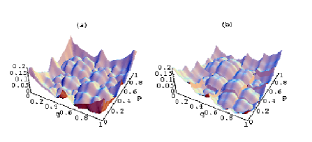
FIG. 1.: (a) The absolute value of the quantum correlation with the $\cos(2\pi q)$ operator for $N=100$ whereas (b) corresponds to a semiclassical evaluation of the same.

For the case of $N=100$, we compare in Fig. (1) the full quantum correlation given by Eq. (3) with the final semiclassical evaluation given by Eq. (28). The absolute value of the correlation function is contoured and superposed on a grey scale. Figure (1a) shows the quantum calculation for the full phase space. In other words, the intensity (value) of each point, $(q,p)$, on the plot represents the $C_{A}(\alpha)$-calculation for a wave packet centered at $(q_{\alpha}=q,p_{\alpha}=p)$. The first sum in Eq. (28) (over $T_{1}$ terms) is a smooth function, and it also displays an additional symmetry about $1/2$ in both canonical variables separately. This extra symmetry is broken by the second sum (over $T_{2}$ terms). Figure 1(b) compares the semiclassical formula to the exact quantum calculation. We have taken eight “forward” correlations (excluding zero), i.e. $T_{1}=8$, while we have only taken two “backward” correlations, i.e. $T_{2}=2$. This is because it appears that the approximations that go into the latter expressions lead to non-uniformly converging quantities and it works better to stop at a earlier point in the series. The (artificial) discontinuities at $1/2$ and $1/4$ are seen prominently in the semiclassical results. Otherwise, it turns out that the semiclassical approximation captures many fine-scale features of the correlations, some of which will be discussed below. Figures (2a,b) are for specific one dimensional sections of the same quantities. The agreement is very good.

FIG. 2.: Sections of the correlation for $N=100$. (a) $p_{\alpha}=.33$ section, (b) $p_{\alpha}=.72$ section. The points are the quantum calculation while the solid lines are semiclassical evaluations.

D Classical features in the correlation

A strong (positive) correlation is indicated at the classical fixed points $(0,0)$ and $(1,1)$, with the rest of the significant correlations being negative. They are dominated by several classical structures as illustrated in Fig. (3). Here the $N$ value used is 200, and superposed on the significant contour features are the following classical orbits:

• the period-2 orbit at $(1/3,2/3)$, $(2/3,1/3)$ is by far the most prominent structure. This is shown in Fig. (3a) by two circular dots. Also, we can look at these structures closely through 1-d slices. In Fig. (2a), the correlation is seen to be large and negative at $(q_{\alpha}=.66)$. The period-2 structure is dominating the landscape;

• next in importance is the primary homoclinic orbit to the period 2 orbit in i), $(1/3,1/3)$, which goes to $(2/3,1/6)$, quickly gets into the region of the period two orbit and is difficult to resolve. The parity and time-reversal symmetric image points are also indicated. It turns out that there is an infinite set of periodic orbits which approximate this orbit more and more closely. Its effects may be present simultaneously, and indistinguishable from the homoclinic orbit itself [12]. The relevant family (set) is denoted by $(001)_{01}$ which is based on a complete binary coding of the orbits [25]. For example, the first few periodic orbits of the family are associated with the binary codes $(00101)$, $(0010101)$, and $(001010101)$. They are also shown in Fig. (3b), including the symmetric image points. In the 1-d slice of Fig. (2a) we see this orbit as well;

  

  FIG. 3.: Comparison of classical structures in the correlation at $N=100$. Details in the text.

• there is an infinite number of orbits homoclinic to the period-2 orbit. They become increasingly more complicated. The next associated periodic orbit family, $(0011)_{01}$, is shown in Fig. (3c), including the symmetric image points. This family was noted by Saraceno to scar eigenfunctions [12]. Also shown in this figure is the period-4 along the diagonal lines: $(3/5,3/5)\rightarrow(1/5,4/5)\rightarrow(2/5,2/5)\rightarrow(4/5,1/5)$. Figure (4) shows sections at $p_{\alpha}=3/5,4/5,2/5$ to highlight this orbit. In Figs. (4a) $p_{\alpha}=3/5$ and has a local minimum at $q_{\alpha}=3/5$; (b) $p_{\alpha}=4/5$ and has a local minimum at $q_{\alpha}=1/5$; and (c) $p_{\alpha}=2/5$ and has a local minimum at $q_{\alpha}=2/5$. These are marked, to indicate location along $q_{\alpha}$ by filled circles. The other minima are due to competing nearby structures of the period-2 orbit and its principal homoclinic excursion;

  

  FIG. 4.: Sections of the correlation ($N=100)$ to highlight the period-4 orbit. (a) $p_{\alpha}=3/5$ and has a local minimum at $q_{\alpha}=3/5$ (b) $p_{\alpha}=4/5$ and has a local minimum at $q_{\alpha}=1/5$ (c) $p_{\alpha}=2/5$ and has a local minimum at $q_{\alpha}=2/5$.

• the orbit homoclinic to the period-4 orbit included in Fig. (3c) with the initial condition $(1/5,2/5)$ (and its symmetric partners) is shown in Fig. (3d); and

• points, such as $(0,1/4)$, which are homoclinic to the fixed points $(0,0)$, $(1,1)$ also show prominently.

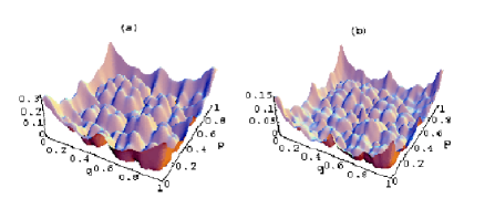
FIG. 5.: The correlation at (a) $N=128$ and (b) $N=200$. Note the sharp features in (a), where the peak height is about twice as large as that in (b).

That these structures are in a sense invariant, i.e. not specific to $N=100$ is shown in Fig. (5a,b) where the correlation (absolute value) is shown for $N=128$ and $200$ respectively. The phase-space resolution of the correlation is increasing with $N$, while the overall magnitude is decreasing as $1/N$. The peculiar properties of the quantum bakers map for N equaling a power of two [25, 12, 29] is tested by $N=128$. Here the correlation is “cleaner” and the stable and unstable manifolds at 1/4, 1/2, and 3/4 of the fixed points are clearly visible. The peaks are well enunciated as well. Both Figs. (5a,b) have contours up to 2/3 peak height, so a direct comparison is meaningful. Higher $N$ values show more clearly the secondary homoclinic orbit to the period-2 orbit.

We may compare these structures with the inverse participation ratio defined as:

$$P(\alpha)\,=\,\sum_{i=0}^{N-1}\left|\langle\alpha|\psi_{i}\rangle\right|^{4}.$$ (29)

It is illustrated in Fig. (6). It shows marked enhancements at the period-2 and period-4 (along the symmetry lines) orbits, and closer examination reveals all orbits up to period-4 are present and one orbit of period-6 along the symmetry lines (the diagonals); see Ref. [29] for a more detailed discussion.

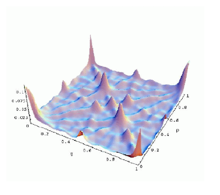
FIG. 6.: The participation ratio for the bakers map. Classical structures are present in this quantity as well.

E General operators and selective enhancements

The results so far have dealt with the special case $A(q)=\cos(2\pi q)$. It seems natural to suspect that the structures highlighted in the correlation are dependent on the choice of the operator. This turns out to be true, and we show here how this works in the bakers map. We reemphasize though that were the eigenstates behaving ergodically, the correlations would have been consistent with zero to within statistical uncertainties independent of the choice of the operator. In this sense, a complete view of the extent to which the eigenstates manifest phase space localization properties comes only from considering both the full phase plane of wave packets and enough operators to span roughly the space of possible perturbations of the energy surface. The flexibility of operator choice does provide a means to enhance selectively particular features of interest supposing one had a specific localization question in mind. As an illustration, note that localization about the period-3 orbit barely appeared in the contour plot of Fig. (3), and yet, we show below that it can be made to show up prominently with other operators.

FIG. 7.: The correlation for the series of operators $A=cos(2\pi 2^{m}q)$. Shown are $m=0$ (large dot), $m=1$ (small dot), $m=2$ (dashed line).

Since the case $A(q)=\sin(2\pi nq)$ has vanishing correlations for any integer $n$ due to symmetry, the other cases of interest are the higher harmonics of the cosine. Therefore consider:

$$A(q)=\cos(2\pi nq).$$ (30)

If $n=2^{m}$ for some positive integer $m$, a rather remarkable scaling property of the quantum bakers map is revealed that is actually implicit in the way the bakers map was originally quantized in [25]. Semiclassically, the correlations are identical to the case $m=0$. For example, consider $A(q)=\cos(4\pi q)$. Then the one-step back classical correlation becomes identical to the zero-th order correlation corresponding to $A(q)=\cos(2\pi q)$. The correlations all shift by $m$ in the sense that $C(l)\longrightarrow C(l+m)$. Thus, there is a kind of scale invariance in the correlation like classical fractals, although this is not self-similarity in the same curve. Quantum calculations reflect this invariance to a remarkable degree as seen in Fig. (7) where the $N=200$ and $p_{\alpha}=1/3$ case is shown.

Other harmonics do weight differently the same localization effects (classical structures). In Fig. (8), $N$ and $p_{\alpha}$ are taken the same as in Fig. (7). The cases $n=1,3,5$ are all very different from each other, but note that the case $n=6$ almost coincides with $n=3$ for the same reason that powers of two harmonics are nearly same. Thus only operators of odd harmonics give the possibility of providing new or unique information about the nonergodicity in the eigenstates. The period-2 orbit localization is accentuated at $n=3$, since for $n=3m$ where $m$ is a positive integer, $\cos(6\pi mq)$ has a maximum of $+1$ at $q=2/3$, whereas for all other integers $n$, $\cos(2\pi nq)=-1/2$ at the same point. In short the perturbation (or measurement) is more significant at the location of the period-2 orbit for $n=3$. On the other hand, the case $n=5$ is similar to the fundamental harmonic case at $q=2/3$ where the perturbation is also equal to $-1/2$.

FIG. 8.: Correlation for different harmonics $A=cos(2\pi nq)$. Shown are $n=1$ (solid large dots), $n=3$ (solid line), $n=5$ (dotted line), and $n=6$ (dashed line).

The case $n=7$ is interesting as $\cos(14\pi q)$ has a maximum at $q=1/7$ which coincides with a period-3 orbit at $(1/7,4/7)$. In Fig. (9), we see the correlation ($N=100)$ corresponding to this operator and the dominant structure is this period-3 orbit and its symmetric partner. Also visible are the stable and unstable manifolds of these orbits. In fact, it is the multiples of the $2^{m}-1$ harmonics which selectively highlights the period $m$ orbits.

Summarizing then, the correlations reflect that the bakers map eigenstates are not ergodic, and manifest strongly phase space localization properties. There do not exist transport barriers such as cantori or diffusive dynamics in the bakers map, so whatever localization that exists should be due to scarring by the short periodic orbits. This is confirmed in the examples shown with connections to their homoclinic orbits illustrated as well. The perturbation or observable determines the regions of phase space that will light up in the correlation measure. A semiclassical theory predicts reasonably well many of these structures. The correlation is semiclassically written as a sum of classical correlations that are super-exponentially cut off after about half the log-time scale.

FIG. 9.: The correlation for the operator $A=cos(14\pi q)$ and case $N=100$. The highlighted areas are in the region of classical period-3 orbits.

III The standard map

A The map and the mixed phase space regime

The standard map (a review is found in [35]) has many complications that can arise in more generic models and we turn to their study. It is also an area-preserving, two-dimensional map of the cylinder onto itself that may be wrapped on a torus. We will consider identical settings of the phase space and Hilbert space as for the bakers map discussed above. The standard map has a parameter that controls the degree of chaos and thus we can study the effect of regular regions in phase space, i.e. the generic case of mixed dynamics.

The classical standard map is given by the recursion

$$q_{i+1} = (q_{i}+p_{i+1})\,\mbox{mod}\,(1)$$ (31)

$$p_{i+1} = (p_{i}-(k/2\pi)\sin(2\pi q_{i}))\,\mbox{mod}\,(1),$$ (32)

where $i$ is the discrete time. The parameter $k$ is of principal interest and it controls the degree of chaos in the map. Classically speaking, an almost complete transition to ergodicity and mixing is attained above values of $k\approx 5$, while the last rotational KAM torus breaks around $k\approx.971$.

The quantum map in the discrete position basis is given by [36]

$$\langle n|U|n^{\prime}\rangle\, = \,\frac{1}{\sqrt{iN}}\exp\left(i\pi(n-n^{\prime})^{2}/N\right)$$ (34)

$$\times\exp\left(i\frac{kN}{2\pi}\cos(2\pi(n+a)/N)\right).$$

The parameter to be varied will be the “kicking strength” $k$, while the phase $a=1/2$ for maximal quantum symmetries, and $n,n^{\prime}\,=\,0,\ldots,N-1$.

We use the unitary operator and evaluate the correlation as in Eq. (3) with $A(q)=\cos(2\pi q)$ here as well. This corresponds exactly to the level velocity induced by a change in the parameter $k$. In Fig. (10) is shown the absolute value of the correlation for various values of parameter $k$. Case (a) corresponds to $k=.1\times(2\pi)$ and is dominated by the KAM curves as the perturbation has not yet led to significant chaos. Highlighted is the fixed point resonance region at the origin that is initially stable. An unstable point is located at the point $(1/2,0\ {\rm or}\ 1)$. The separatrix or the stable and the unstable manifolds of this point are aligned along the local ridges seen in the correlation. Also the period-2 resonance region is visible. Higher resolution not shown here, corresponding to higher values of $N$ reveal weakly the period-3 resonance as well. Case (b) corresponds to $k=.3\times(2\pi)$ while (c) and (d) to $k=.9\times(2\pi)$ and $k=2.3\times(2\pi)$ respectively. We note the gradual destruction of the KAM tori and the emergence of structures that are dominated by hyperbolic orbits. A more detailed classical-quantum correspondence is however not attempted here.

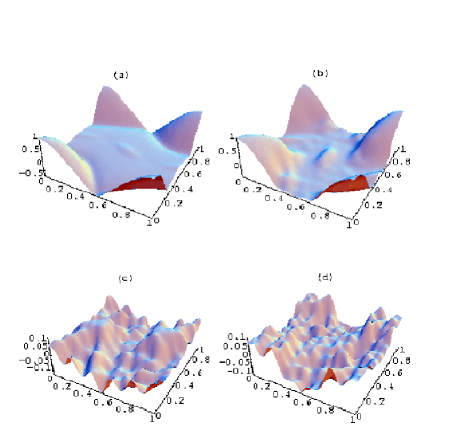
FIG. 10.: The quantum correlation for the standard map ($N=100$), (a) $k/(2\pi)=.1$, (b) $k/(2\pi)=.3$, (c) $k/(2\pi)=.9$, (d) $k/(2\pi)=2.3$.

These contour plots do not reveal the difference in the magnitude between the correlations in the stable and unstable regions. In Fig. (11), we have plotted the correlation at the origin $(0,0)$, which is also a fixed point, as a function of the parameter. The value $k/(2\pi)\sim 1$ corresponds to a transition to complete classical chaos and is reflected in this plot as erratic and small oscillations. The large correlation in the mixed phase space regime arises from the non-ergodic nature of the classical dynamics. The classical fixed point loses stability at $k^{\ast}/(2\pi)=4/(2\pi)\approx.63$ and this is roughly the region at which the correlation starts to dip away from unity toward lower values.

FIG. 11.: The quantum correlation for the standard map at $\alpha=(0,0)$ as a function of the parameter $k$ ($N=100$ is the solid line and $N=200$ is the dashed one). The dotted line is a classical estimate based on Eq. (38) and averaged over twenty time steps with $N=100$.

The gross features and principal $\hbar$ behavior in this regime is easy to derive in terms of purely classical correlations as follows:

$$C_{A}(\alpha)\, = \,\left<\mbox{Tr}\left(|\alpha\rangle\langle\alpha|\hat{A}(n)\right)\right>_{n}\,$$ (35)

$$= \,\left<\int dq\,dp\,[|\alpha\rangle\langle\alpha|]_{W}\,[\hat{A}(n)]_{W}\right>_{n}$$ (36)

where $[.]_{W}$ is the Weyl-Wigner transform of the operator in the brackets and $\hat{A}(n)$ is the operator after a time $n$. Without worrying about the toral nature of the phase space and the Weyl-Wigner transforms, we treat the problem as in a plane. This is justified by the use of localized, Gaussian wave packets. Otherwise, we could imagine that the Wigner transform of the projector would follow from an infinite series of Gaussian states that is equivalent to discretizing the Gaussian. We use a normalized, “circular” Gaussian of width $\sqrt{\hbar}$. The approximation comes in when we replace $[\hat{A}(n)]_{W}$ by $A(f^{n}(q,p))$ where the latter is the classical function evaluated at the classically iterated point $q_{n}=f^{n}(q,p)$. We expect this approximation to be valid in the case of regular dynamics over a much longer time scale than found with chaotic dynamics. To a good approximation,

$$C_{A}(\alpha)\, \sim \,\left<\int dq\,dp\,\left(\frac{1}{\pi\hbar}\right)\exp\left[-\frac{1}{\hbar}\left((q-q_{\alpha})^{2}\right.\right.\right.$$ (38)

$$\left.\left.\left.+(p-p_{\alpha})^{2}\right)\right]\,A\left(f^{n}(q,p)\right)\right>_{n}$$

As intuitively expected, there is no principal $\hbar$ dependence in the correlation since there is a non-zero classical limit. At $\hbar=0$, we could replace the Gaussian forms by $\delta-$functions and would get simply $C_{A}(\alpha)\,=\,\left<A(f^{n}(q_{\alpha},p_{\alpha}))\right>_{n}$.

This however vanishes as the classical system becomes more ergodic and is no more capable of predicting the correlation. Higher-order corrections are needed. It is in this regime that we studied the bakers map and found that the correlation has a principal part that scales (almost) as $\hbar$ and classical correlations based on periodic orbits predict the localization features that arise out of quantum interference.

We return to Fig. (11) to remark on some of these properties. Notice that the simple estimate of Eq. (38) performs very well, even as the phase space is becoming increasingly chaotic. It is quite unexpected that the oscillations after the onset of full mixing (around $k/(2\pi)=1$) should follow this estimate. However, after the transition to chaos the classical estimate will depend on the times over which the averaging is done and as this increases the estimate would vanish.

B Chaotic regime

We attempt in some measure a semiclassical theory for the correlation in the chaotic regime along the lines adopted for the quantum bakers map. Of the two ingredients in Eq. (5) one of them remains the same, namely Eq. (9). However the diagonal elements of the propagator in Eq. (8) have to be generalized.

In [32] a semiclassical expression for the matrix elements of the propagator as a homoclinic orbit sum is given. Although this was derived with the example of the billiard in mind, it can be interpreted as a generalization of Eq. (8) for area-preserving, two-dimensional maps. We, however, interpret the sum not as a homoclinic orbit sum, but as a periodic orbit sum. To each homoclinic orbit there is a neighboring periodic orbit that we will use instead. This will form the points around which the expansions are carried out and the result is identical to that in [32]. Thus we write

$$\langle\alpha|U^{n}|\alpha\rangle\,\sim\,\sum_{\gamma}\exp\left(iS_{\gamma}/\hbar-i\pi\nu/2\right)\sum_{j}B_{j}$$ (39)

where

$$B_{j}\, = \,\sqrt{\frac{2}{A_{0}}}\exp\left\{\frac{-1}{2\hbar A_{0}}\left[(\mbox{tr}-2)(\delta q^{2}+\delta p^{2})\,\right.\right.$$ (41)

$$\left.\left.+\,2i(m_{21}\,\delta p^{2}-m_{12}\,\delta q^{2}+\delta q\delta p\,(m_{22}-m_{11}))\right]\right\}.$$

$B_{j}$ generalizes the Gaussian form (including the prefactor) in Eq. (8). Again $j$ labels points along the periodic orbit and $\delta q=q_{j}-q_{\alpha}$, $\delta p=p_{j}-p_{\alpha}$ are as before deviations from the centroid of the wave packet. The two dimensional matrix elements, $m_{ij}$, are the elements of the stability matrix at the periodic point $j$ along the periodic orbit $\gamma$. The deviations $\delta q$ and $\delta p$ after $n$ iterations of the map are given by:

$$\left(\begin{array}[]{c}\delta p_{n}\\ \delta q_{n}\end{array}\right)\,=\,\left(\begin{array}[]{ll}m_{11}&m_{12}\\ m_{21}&m_{22}\end{array}\right)\left(\begin{array}[]{c}\delta p\\ \delta q\end{array}\right)$$ (42)

The invariant is the trace of this matrix that is denoted tr. While $A_{0}\,=\,m_{11}+m_{22}+i(m_{21}-m_{12})$, $\nu$ is a phase that will not play a crucial role below. In the case of the bakers map $m_{12}=m_{21}=0$ and $m_{11}=2^{-n},\,m_{22}=2^{n}$ uniformly at all points in phase space, as well as $\nu=0$. On substitution of this in Eq. (39) we get Eq. (8).

The dependence on individual matrix elements of the stability matrix complicates the use of this formula in general. However we note that the Gaussian is effectively cutting off periodic points that are not close to $\alpha$ and therefore we may take the $m_{ij}$ elements to be the stability matrix at this point. In the chaotic regime each of the matrix elements grow exponentially with time $n$. Thus we have that $\exp(-\lambda n)\,m_{ij}\rightarrow$ constant, where $\lambda$ is the Lyapunov exponent. We call this saturated constant $m_{ij}$ as well. Below we will assume that the exponential growth has been factored out of these elements. Also we use $\exp(-\lambda n)\,A_{0}\rightarrow a_{0}$. The terms inside the exponential function in Eq. (41) saturate in time $n$ while the prefactor goes as $\exp(-\lambda n/2)$. It follows then that

$$B_{j}\rightarrow\sqrt{\frac{2}{a_{0}}}\exp(-\lambda n/2)\,F(q_{j},p_{j})$$ (43)

where $F(q_{j},p_{j})$ is

$$F(q_{j},p_{j})\, = \,\exp\left\{\frac{-1}{2\hbar a_{0}}\left[(\delta q^{2}+\delta p^{2})\,\right.\right.$$ (44)

$$+\, \left.\left.2i(m_{21}\,\delta p^{2}-m_{12}\,\delta q^{2}+\delta q\delta p\,(m_{22}-m_{11}))\right]\right\}.$$ (45)

Here the $m_{ij}$ elements already have the exponential behavior factored out. For example in the case of the bakers map $m_{22}=1$ while all the other elements are zero and this gives consistently the approximated Gaussian form in Eq. (12). Further steps are identical to the case of the bakers map and leads to the generalization of Eq. (13):

$$C_{A}(\alpha)\,=\,\sqrt{\frac{2}{a_{0}}}\sum_{T}\sum_{l=-M}^{M}\tilde{C}_{T}(l),$$ (46)

where the classical correlations are calculated as in Eq. (14) with the function $F$ being that in Eq. (44). We may then expect all the principal conclusions from the study of the bakers map to be carried over, principally the decrease in the correlation as $\hbar$, the correlations being cut off after half the log-time scale, and the effects of classical orbits.

More detailed analysis in the lines of the special case discussed in case of the bakers map will run into the following difficulties. First, the $m_{ij}$ elements will depend on $\alpha$ in general. Exceptions are uniformly hyperbolic systems such as the cat or sawtooth maps (and, of course, the bakers map). A second difficulty is that the correlations have to be evaluated to half the log-time while classically iterating the map (analytically) over such times is often not possible. The classical correlations that arise in the study of rms values of level velocities [28] involved correlations that exponentially decreased in time while here we are likely to get generalizations of forms such as in Eq. (18) that will require us to go up to log-times. We have calculated the correlations for times 1, -1, and 2 but will not display them as they are by themselves not very useful. A third problem with this form of the generalization is that it is not explicitly real.

FIG. 12.: The quantum correlation for the standard map ($N=100)$ at $\alpha=(0,0)$ as a function of the parameter $k$ (dashed line). The solid line is the semiclassical estimate.

We have used Eq. (46) and for the $m_{ij}$ used either those calculated at one point in phase space (such as the origin) or in fact assumed those that are relevant for the bakers map. While fine structures are not reproduced, the general features are captured equally well in both these approaches. To illustrate the quality of the approximation we again look at the correlation at the point $(0,0)$ as a function of $k$ in Fig. (12) (as in the previous figure). The solid line is the semiclassical prediction based upon using the same $m_{ij}$ values at all values of $k$. It is seen that even with these (over) simplifications the semiclassical expressions capture much of the oscillations with the parameter and the magnitude.

IV Summary and conclusions

We have studied the details of phase space localization present in the quantum time evolution of operators. This was related to a measure of localization involving the correlation between the level velocities and wavefunction intensities. While individual quantum states show well known interesting scars of classical orbits, groups of states weighted appropriately provide both a convenient and important quantity to study semiclassically. We were interested principally in those features whose origins were quantum mechanical. The quantities studied had both a vanishing classical limit as well as vanishing RMT averages.

We studied simple maps as a way to understand the general features that will appear. We found that the operator dictated to a large extent which parts of phase space will display prominent localization features and further that these localization features are often related to classical periodic orbits and their homoclinic structures. The time average of the operator for wave packets was explicitly related semiclassically to classical correlations. These were shown to be cut off super-exponentially after half the log-time in the quantum bakers map. Thus the localization features in quantum systems associated with scars were reproduced using long (periodic) orbits but short time correlations. The localization would disappear in the classical limit as the magnitude of the quantum correlations or time averages are proportional to (scaled) $\hbar$.

General systems were approached using the quantum standard map and complications that would arise were discussed. Also the case of mixed phase space was seen to be well reproduced by a simple classical argument. The generalization to Hamiltonian systems [21] contains many of the features and structures are also (not surprisingly) present in this case.

We gratefully acknowledge support from the National Science Foundation under Grant No. NSF-PHY-9800106 and the Office of Naval Research under Grant No. N00014-98-1-0079.

REFERENCES

- [1] M. V. Berry, J. Phys. A 10, 2083 (1977).
- [2] A. Voros, In Stochastic Behaviour in Classical and Quantum Hamiltonian Systems, edited by G. Casati and J. Ford (Springer, Berlin, 1979)
- [3] E. B. Stechel and E. J. Heller, Ann. Rev. Phys. Chem. 35, 563 (1984); E. B. Stechel, J. Chem. Phys. 82, 364 (1985).
- [4] L. Kaplan and E. J. Heller, Physica D 121, 1 (1998); Ann. Phys. (N. Y.) 264, 171 (1998); L. Kaplan, Phys. Rev. Lett. 80, 2582 (1998).
- [5] N. L. Balazs and B. K. Jennings, Physics Reports 104 (6), 347 (1984).
- [6] E. J. Heller, Phys. Rev. Lett. 53, 1515 (1984).
- [7] E. J. Heller, in Les Houches LII, Chaos and Quantum Physics, edited by M.-J. Giannoni, A. Voros, and J. Zinn-Justin (North-Holland, Amsterdam 1991).
- [8] E. J. Heller, in Quantum Chaos and Statistical Nuclear Physics, edited by T. H. Selgman and H. Nishioka, Lecture Notes in Physics 263. (Springer, Berlin, 1986).
- [9] E. B. Bogomolny, Physica D 31, 169 (1988).
- [10] M. V. Berry, Proc. R. Soc. Lond. A 423, 219 (1989).
- [11] B. Eckhardt, G. Hose, E. Pollak, Phys. Rev. A 39, 3776 (1989).
- [12] M. Saraceno, Ann. Phys. (N. Y.) 199, 37 (1990).
- [13] M. S. Santhanam, V. B. Sheorey, and A. Lakshminarayan, Phys. Rev. E 57, 345 (1998).
- [14] T. M. Fromhold et al., Phys. Rev. Lett. 72, 2608 (1994).
- [15] G. Muller et al., Phys. Rev. Lett. 75, 2875 (1995).
- [16] R. S. McKay and J. D. Meiss, Phys. Rev. A 37, 4702 (1988).
- [17] R. Ketzmerick, G. Petshel, and T. Geisel, Phys. Rev. Lett. 69, 695 (1995).
- [18] O. Bohigas, S. Tomsovic, and D. Ullmo, Physics Reports 223 (2), 43 (1993).
- [19] S. Tomsovic and E. J. Heller, Phys. Rev. Lett. 70, 1405 (1993).
- [20] S. Tomsovic, Phys. Rev. Lett. 77, 4158 (1996).
- [21] N. R. Cerruti, A. Lakshminarayan, J. H. Lefebvre, and S. Tomsovic, submitted to Phys. Rev. E.
- [22] O. L. De Lange and R. E. Raab, Operator Methods in Quantum Mechanics, (Oxford Science Publications, Oxford, 1991).
- [23] J. Schwinger, Quantum Kinematics and Dynamics, (Benjamin, New York, 1970).
- [24] J. H. Hannay and M. V. Berry, Physica D 1, 267 (1980).
- [25] N. L. Balazs and A. Voros, Ann. Phys. (N. Y.) 190, 1 (1989).
- [26] P. W. O’Connor, S. Tomsovic and E. J. Heller, Physica D 55, 340 (1992).
- [27] T. A. Brody, J. Flores, J. B. French, P. A. Mello, A. Pandey, and S.S.M. Wong, Rev. Mod. Phys. 53, 385 (1981).
- [28] A. Lakshminarayan, N. R. Cerruti and S. Tomsovic, Phys. Rev. E 60, 3992 (1999).
- [29] P. W. O’Connor and S. Tomsovic, Ann. Phys. (N. Y.) 207, 218 (1991).
- [30] A. M. Ozorio de Almeida and M. Saraceno, Ann. Phys. (N. Y.) 210, 1 (1991).
- [31] M. Saraceno and A. Voros, Physica D 79, 206 (1994).
- [32] S. Tomsovic and E. J. Heller, Phys. Rev. E 47, 282 (1993).
- [33] B. Eckhardt, S. Fishman, K. Muller and D. Wintgen, Phys. Rev. A 45, 3531 (1992).
- [34] J. H. Hannay and A. M. Ozorio de Almeida, J. Phys. A 17, 3429 (1984).
- [35] F. M. Izrailev, Phys. Rep. 196, 299 (1990).
- [36] A. Lakshminarayan, Pramana 48, 517 (1997).