[

Statistical geometry in scalar turbulence

Abstract

A general link between geometry and intermittency in passive scalar turbulence is established. Intermittency is qualitatively traced back to events where tracer particles stay for anomalousy long times in degenerate geometries characterized by strong clustering. The quantitative counterpart is the existence of special functions of particle configurations which are statistically invariant under the flow. These are the statistical integrals of motion controlling the scalar statistics at small scales and responsible for the breaking of scale invariance associated to intermittency.

]

Scalar fields transported by turbulent flow occur in many physical situations, ranging from the dynamics of the atmosphere and the ocean to chemical engineering (see, e.g., Ref. [1]). Specific examples are provided by pollutant density, temperature or humidity fields and the concentration of chemical or biological species. The advection-diffusion equation governing the transport of the scalar field $\theta$ is :

$$\partial_{t}\theta({\mbox{\boldmath$r$}},t)+\left({\mbox{\boldmath$v$}}\cdot{\mbox{\boldmath$\nabla$}}\right)\theta({\mbox{\boldmath$r$}},t)=\kappa\Delta\theta({\mbox{\boldmath$r$}},t),$$ (1)

where ${\mbox{\boldmath$v$}}({\mbox{\boldmath$r$}},t)$ is the incompressible advecting flow and $\kappa$ is the molecular diffusivity. Two broad cases are distinguished : active scalars, where $v$ depends on $\theta$, e.g. by an explicit relation ${\mbox{\boldmath$v$}}={\mbox{\boldmath$v$}}\left(\theta\right)$, and passive scalars, where the statistics of $v$ is independent of $\theta$. Here, we shall be concerned with the latter, although we conjecture that the physical mechanisms presented in the following are quite general and relevant also for the active cases. The Fokker-Planck equation (1) is associated to the Lagrangian dynamics of tracer particles whose position ${\mbox{\boldmath$\rho$}}(t)$ obeys $d{\mbox{\boldmath$\rho$}}(t)={\mbox{\boldmath$v$}}({\mbox{\boldmath$\rho$}}(t),t)\,dt+\sqrt{2\kappa}\,\,d{\mbox{\boldmath$\beta$}}(t)$, where ${\mbox{\boldmath$\beta$}}(t)$ is the isotropic Brownian motion [2]. The equation (1) governs the evolution of the probability density of particles at position $r$ and time $t$.

Scalar turbulence is typically generated by maintaining a mean scalar gradient $\langle\theta\rangle={\mbox{\boldmath$g$}}\cdot{\mbox{\boldmath$r$}}$, e.g. by heating/cooling devices in temperature field experiments. The notation $\langle\bullet\rangle$ denotes the average with respect to the velocity statistics, which is in principle arbitrary. We shall be interested in flows with correlations having a nontrivial power law behavior in the inertial range of scales $r\ll L$, where $L$ is the velocity correlation length. Examples are provided by the two and three dimensional Navier-Stokes turbulent flow (see, e.g., Ref. [3]). A very robust feature of scalar turbulence is its strong intermittency : rare strong events (such as the sharp cliffs observed in Fig. 1) dominate the scalar statistical properties. More quantitatively, intermittency reflects in the anomalous scaling of the correlations. In the inertial range, the scalar structure functions $S_{n}({\mbox{\boldmath$r$}})=\langle\left(\theta({\mbox{\boldmath$r$}},t)-\theta({\mbox{\boldmath$0$}},t)\right)^{n}\rangle$ take the form

$$S_{n}({\mbox{\boldmath$r$}})\propto r^{\zeta_{n}^{dim}}\,\,\left({L\over r}\right)^{\zeta_{n}^{dim}-\zeta_{n}},$$ (2)

with a nonvanishing value of $\zeta_{n}^{dim}-\zeta_{n}$. Here, $\zeta_{n}^{dim}$ is the value predicted by simple mean field dimensional arguments, e.g. of the Kolmogorov 1941 type. The positive value of the anomalous correction $\zeta_{n}^{dim}-\zeta_{n}$ reflects the breaking of scale-invariance : the scale $L$ explicitly appears in the inertial range expressions of scalar correlations, even though $r\ll L$. The phenomenon of intermittency is quite generic for scalar turbulence and independent of the specific choice of $v$, including for Gaussian velocity fields (see, e.g., Ref. [1]). Past research on intermittency has mostly concentrated on phenomenological models making vague contacts with the dynamics and based uniquely on scaling exponents and structure functions. Angular dependencies and geometrical informations about the correlations were discarded. It is shown here that the whole structure of multi-point correlations is in fact needed to achieve a real dynamical understanding based on the geometry of the figures identified by tracer particles. Deviations of exponents from naïves dimensional values turn out to be just by-products of the figure geometry nontrivial evolution under Lagrangian dynamics. While the figure size grows according to simple dimensional arguments, the evolution of their shape is a more delicate issue. There are in particular some special functions of the particle positions whose average with respect to the Lagrangian dynamics remains constant in time. That is due to a delicate compensation between the growth due to the figure size and the depletion associated to the figure shape. Those statistically conserved functions are dominating the behavior in the inertial range and controlling the scalar field intermittency.

Specifically, the velocity field $v$ considered here is a two-dimensional turbulent flow generated by an inverse energy cascade process [4]. This is a situation of interest both for experiments [5, 6] and in the atmosphere [7, 8]. The flow realizes the type of turbulence theoretically postulated by A.N. Kolmogorov in 1941 : it is isotropic, it has a constant energy flux (but upscale) and it is scale-invariant with scaling exponent $1/3$ [5, 9]. A property of interest to us is that the velocity is not intermittent. All nontrivial scaling properties of the scalar field presented in the following are therefore entirely due to the

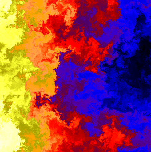
FIG. 1.: A snapshot of the scalar field obtained by numerical integration of (1) with advection by a two-dimensional turbulent flow generated by an inverse energy cascade. The scalar turbulence is maintained by a fixed temperature gradient $\langle\theta\rangle={\mbox{\boldmath$g$}}\cdot{\mbox{\boldmath$r$}}$, with $g$ oriented from right to left.

advection-diffusion equation (1) and not mere footprints of the velocity field. Details on the integration procedure used for the numerical simulations of (1) with a mean gradient $g$ can be found in Ref. [10]. The single-time scalar statistics at the stationary state is defined by the $n$-point correlations $C_{n}(\underline{\mbox{\boldmath$r$}},t)=\langle\theta({\mbox{\boldmath$r$}}_{1},t)\cdots\theta({\mbox{\boldmath$r$}}_{n},t)\rangle$, where $\underline{\mbox{\boldmath$r$}}$ denotes the set ${\mbox{\boldmath$r$}}_{1},\ldots,{\mbox{\boldmath$r$}}_{n}$. For spatially homogeneous situations, $C_{n}$ is invariant under translations and it depends only on $2n-2$ degrees of freedom, associated to the separation vectors among the $n$ points. In the inertial range, the velocity scale invariance is expected to reflect in scalar correlations $C_{n}(\underline{\mbox{\boldmath$r$}})$ behaving as power laws with respect to global size variables, such as e.g. the gyration radius of the set $\underline{\mbox{\boldmath$r$}}$.

Let us consider for simplicity the third order case $n=3$. All the following arguments are easily generalized to higher order correlations. The correlation function $C_{3}$ depends on the size, the orientation and the shape of the triangle defined by the three points ${\mbox{\boldmath$r$}}_{1}$, ${\mbox{\boldmath$r$}}_{2}$ and ${\mbox{\boldmath$r$}}_{3}$. The global size variable can be defined as $R^{2}=(r_{12}^{2}+r_{23}^{2}+r_{31}^{2})/3$, where $r_{ij}$ is the distance between the $i$-th and the $j$-th particle. As shown in Fig. 2, in the inertial range of scales $C_{3}$ depends on $R$ as a power law with the exponent $\zeta_{3}=1.25$. The hallmark of intermittency is in the fact that $\zeta_{3}$ is smaller than the dimensional prediction $5/3$ (see Ref. [1]). As for the shape and the orientation of the triangle, we shall use the same Euler parametrization as in Refs. [11, 12]. Defining ${\mbox{\boldmath$\rho$}}_{1}=\left({\mbox{\boldmath$r$}}_{1}-{\mbox{\boldmath$r$}}_{2}\right)/\sqrt{2}$ and

FIG. 2.: The dependence of the third order correlation function $C_{3}$ with respect to the size of the triangle $R$. The straight line is the power law behavior $R^{1.25}$.

${\mbox{\boldmath$\rho$}}_{2}=\left({\mbox{\boldmath$r$}}_{1}+{\mbox{\boldmath$r$}}_{2}-2{\mbox{\boldmath$r$}}_{3}\right)/\sqrt{6}$, the shape of the triangle is controlled by the two variables

$$\chi=1/2\tan^{-1}\left[{2{\mbox{\boldmath$\rho$}}_{1}\cdot{\mbox{\boldmath$\rho$}}_{2}\over(\rho_{1}^{2}-\rho_{2}^{2})}\right]\,;\quad w=2{|{\mbox{\boldmath$\rho$}}_{1}\times{\mbox{\boldmath$\rho$}}_{2}|\over R}.$$ (3)

Some of the shapes associated to different values of $\chi$ and $w$ are shown in Fig. 2. The global orientation of the triangle with respect to the mean gradient direction $g$ is defined by the angle $\varphi$. It is convenient to decompose $C_{3}$ on the orthogonal basis made of $\cos\left(\ell\varphi\right)$ and $\sin\left(\ell\varphi\right)$. Reversing the coordinates with respect to an axis parallel or orthogonal to $g$ statistically leaves the $\theta$ field invariant or inverts its sign, respectively. In the projection of $C_{3}$, the angular momentum $\ell$ should therefore be odd and sine functions are absent. Furthermore, the dominant contribution at the small scales is the one having the lowest angular momentum (see Ref. [13] for the case of Navier-Stokes turbulence). The correlation function $C_{3}$ takes then the form

$$C_{3}(\underline{\mbox{\boldmath$r$}})=R^{\zeta_{3}}\,f(\chi,w)\,\cos\varphi+\ldots\;,$$ (4)

where the dots stand for subdominant higher-order harmonics of the form $\cos(2\ell+1)\varphi$. The invariance under arbitrary permutations of the three vertices of the triangle allows to reduce the phase space to $-\pi/6<\chi<\pi/6$, $0<w<1$ and the function $f$ in (4) is antiperiodic in $\chi$ with period $\pi/3$ [11, 12]. The measured dependence of $f$ on the shape coordinates $\chi$ and $w$ is shown in Fig. 3. The maximum of $f$ is realized at $\chi=0$, $w=0$, where two of the three particles are stuck together. For equilateral triangles ($w=1$) or for the “dumbbell” configuration $\chi=\pi/6$, $w=0$, the symmetries enforce $f=0$.

Let us establish the connection with the Lagrangian dynamics. That is done by replacing the Eulerian variables $\underline{\mbox{\boldmath$r$}}$ in the argument of $C_{3}$ by their Lagrangian evolutions $\underline{\mbox{\boldmath$\rho$}}(t)$, with $\underline{\mbox{\boldmath$\rho$}}(0)=\underline{\mbox{\boldmath$r$}}$. The resulting object is a

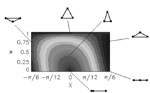
FIG. 3.: Contour lines in the $\chi\,-\,w$ plane of the third order shape function $f$ appearing in (5).

stochastic function whose average with respect to the Lagrangian trajectory statistics is denoted by $\langle\bullet\rangle_{\cal L}$. More generally, for a generic function $\phi(\underline{\mbox{\boldmath$r$}})$ of the $n$ points ${\mbox{\boldmath$r$}}_{i}$ we can define its Lagrangian average as

$$\langle\phi(t)\rangle_{\cal L}=\int\phi(\underline{\mbox{\boldmath$\rho$}})P_{n}\left(t\,,\underline{\mbox{\boldmath$\rho$}}\big{|}0\,,\underline{\mbox{\boldmath$r$}}\right)\,d\underline{\mbox{\boldmath$\rho$}}.$$ (5)

Here, the $n$-particle propagator $P_{n}\left(t\,,\underline{\mbox{\boldmath$\rho$}}\big{|}0\,,\underline{\mbox{\boldmath$r$}}\right)$ denotes the probability that, being in $\underline{\mbox{\boldmath$r$}}$ at time $0$, the $n$ particles are in $\underline{\mbox{\boldmath$\rho$}}$ at time $t$. In a turbulent Kolmogorov flow, distances typically grow with time as $|t|^{3/2}$, whose special instance is the celebrated Richardson law $\langle r_{12}^{2}\rangle_{\cal L}(t)\propto|t|^{3}$ for the distance $r_{12}$ between two particles. For generic functions $\phi$, homogeneous of positive degree $\sigma$ that is $\phi(\lambda\underline{\mbox{\boldmath$r$}})=\lambda^{\sigma}\phi(\underline{\mbox{\boldmath$r$}})$, the Lagrangian average is therefore expected to grow as $|t|^{3\sigma/2}$.

Intermittency is dynamically originated by blatant violations of expectations à la Richardson. The anomalous part of correlation functions has in fact a constant Lagrangian average, as clearly demonstrated in Fig. 4 for the third order case. Those statistically preserved functions are the statistical integrals of motion responsible for the breaking of scale invariance associated to intermittency. The other important point is that their constancy is tightly related to the geometry of the figures identified by the Lagrangian particles. Fig. 4 indicates indeed that the size factor $R^{\zeta_{3}}$ grows as $|t|^{3\zeta_{3}/2}$. The Lagrangian average of $C_{3}$ remaining constant, the shape part $f(\chi,w)\,\cos\varphi$ in (4) must compensate for the growth of the figure size. As shown in Fig. 3, the function $f$ decreases going from degenerate triangles with two of the vertices close to each other to triangles with aspect ratios of order unity. The geometrical meaning of anomalous scaling laws is then quite clear : the smaller is $\zeta_{3}$, the slower is the compensation needed from the shape factor and the longer degenerate triangle configurations persist. In other words, “stronger intermittency = particles staying longer close to each other”.

FIG. 4.: The Lagrangian average of the correlation function $\langle C_{3}\rangle_{\cal L}$. For comparison, it is also shown the evolution of the average $\langle R^{\zeta_{3}}\rangle_{L}\sim|t|^{{3\over 2}\zeta_{3}}$, that obeys the dimensional scaling law.

Systematic support to the previous physical ideas can be provided in the special case where the advecting velocity in (1) has a short correlation time, the so-called Kraichnan model [14]. The assumption is of course far from realistic, but it leads to the peculiar property that the $n$-particle propagators $P_{n}$ in (5) obey closed Fokker-Planck equations [15] (see also Ref. [1]). The statistically preserved functions are now identified as zero modes of the $n$-particle Fokker-Planck operator [16, 17, 18]. Their anomalous scaling behavior could be calculated in some perturbative limits [16, 17, 18] or measured numerically [19, 20]. Zero modes enter the $P_{n}$’s via the asymptotic expansion [21] (see also Ref. [22]) :

$$P_{n}\!\!\left(t,\underline{\mbox{\boldmath$\rho$}}\Big{|}0,\lambda\,\,\underline{\mbox{\boldmath$r$}}\right)\!\!\!=\!\!\sum_{i,q}\,\,\lambda^{\sigma_{i,q}}\phi_{i,q}(\underline{\mbox{\boldmath$r$}})\,\psi_{i,q}(t,\underline{\mbox{\boldmath$\rho$}}),$$ (6)

valid for small $\lambda$’s. Zero modes are the $q=0$ terms in (6) and they are ordered according to their scaling dimension by the index $i$. Higher $q$’s identify the so-called slow modes, whose Lagrangian average is growing as an integer power of time, although with an exponent smaller than the dimensional one $3\sigma_{i,q}/2$.

A simple example of slow mode for our inverse cascade velocity field is provided for $n=2$. The Lagrangian average of $\left({\mbox{\boldmath$g$}}\cdot{\mbox{\boldmath$r$}}_{12}\right)$ is preserved as its time derivative is proportional to $\langle\left({\mbox{\boldmath$v$}}_{1}-{\mbox{\boldmath$v$}}_{2}\right)\rangle=0$. The first slow mode associated to it is given by the function $\left({\mbox{\boldmath$g$}}\cdot{\mbox{\boldmath$r$}}_{12}\right)\,{r_{12}^{2/3}}$. Fig. 5 shows indeed that its Lagrangian average grows as $|t|$, much slower at large times than the dimensional law $|t|^{5/2}$.

What is the degree of generality of the Lagrangian preservation mechanism for intermittency and the expansion (6) ? The crucial property of the Kraichnan velocity field is its short correlation time (this ensures that the

FIG. 5.: The Lagrangian average of the anisotropic slow mode $\left({\mbox{\boldmath$g$}}\cdot{\mbox{\boldmath$r$}}_{12}\right)\,{r_{12}^{2/3}}$ vs time.

Lagrangian trajectories are Markovian). For the inverse energy cascade flow considered here this property is lost as the correlation time is finite. The numerical results presented here give therefore a strong indication that the basic mechanisms for scalar intermittency are quite robust and generic. Changing the statistics of the flow affects only quantitative details, such as the numerical value of the exponents or the precise shape of the Lagrangian preserved functions. The expansion (6) is analogous to those encountered in many-body statistical problems [23] and controls the small-scale behavior of scalar correlations. Indeed, it follows from (1) that the scalar is preserved along the Lagrangian trajectories. Scalar correlations can be then expressed as

$$C_{n}(\underline{\mbox{\boldmath$r$}},t)=\int P_{n}\left(-t,\underline{\mbox{\boldmath$\rho$}}\big{|}0,\underline{\mbox{\boldmath$r$}}\right)\left({\mbox{\boldmath$g$}}\cdot{\mbox{\boldmath$\rho$}}_{1}\right)\ldots\left({\mbox{\boldmath$g$}}\cdot{\mbox{\boldmath$\rho$}}_{n}\right)d\underline{\mbox{\boldmath$\rho$}}.$$ (7)

Inserting (6) into this expression it is evident that the behavior at small scales is a superposition of the functions $\phi_{i,q}$. Two general remarks on scalar turbulence follow. First, changing the initial condition ${\mbox{\boldmath$g$}}\cdot{\mbox{\boldmath$r$}}$ (or the injection mechanism in the forced case) modifies the constants but not the scaling exponents in the correlation functions. This naturally explains the universality properties of scalar turbulence observed in Ref. [10]. Second, all fewer-particle modes $\phi_{i,q}$, i.e. those depending on $m<n$ variables, appear in the expression for $C_{n}$. Their Lagrangian averages with respect to the evolution of the $m$ particles or the whole set of $n$ particles are indeed trivially coinciding. Note however that structure functions satisfy the trivial identity $S_{n}(r)=\int_{0}^{r}\ldots\int_{0}^{r}\partial_{r_{1}}\ldots\partial_{r_{n}}C_{n}(\underline{r})\,d\underline{r}$. All $m$-particle modes will therefore drop out from the $n$-th order structure function. This clearly illustrates a point previously mentioned : the apparent simplification of the single distance $r$ left in structure functions is purely illusory as their anomalous scaling laws are still dynamically associated to $n$-particle geometries.

In conclusion, we have identified the integrals of motion responsible for the failure of dimensional analysis and intermittency in scalar turbulence. The anomalous parts of correlation functions are preserved under the Lagrangian dynamics. That preservation is a geometrical effect associated to figures identified by scalar particles persisting in degenerate shapes. Particles tend indeed to remain close to each other for unexpectedly long times, pointing to applications for the reaction rate enhancement in the transport of chemically reactive species.

Acknowledgments We are grateful to U. Frisch and K. Gawȩdzki for illuminating discussions. A. Celani was supported by a “H. Poincaré” CNRS postdoctoral fellowship. The work was partially supported by the EU contract HPRN-CT-2000-00162 “Nonideal Turbulence” and the NSF under Grant No. PHY94-07194.

REFERENCES

- [1] B.I. Shraiman & E. Siggia, “Scalar Turbulence”, Nature, (2000) to appear.
- [2] H. Risken, The Fokker-Planck equation, Springer-Verlag, 2nd ed. (1996).
- [3] U. Frisch, Turbulence. The Legacy of A.N. Kolmogorov, Cambridge Univ. Press, Cambridge, (1995).
- [4] R.H. Kraichnan, Phys. Fluids, 10, 1417, (1967).
- [5] J. Paret & P. Tabeling, Phys. Fluids, 10, 3126, (1998).
- [6] M. A. Rutgers, Phys. Rev. Lett., 81 (1998) 2244.
- [7] K.S. Gage, J. Atmos. Sci., 36, 1950, (1979).
- [8] E. Lindborg, J. Fluid Mech., 388, 259, (1999).
- [9] G. Boffetta, A. Celani & M. Vergassola, Phys. Rev. E, 61, R29, (2000).
- [10] A. Celani, A. Lanotte, A. Mazzino & M. Vergassola, Phys. Rev. Lett. 84, 2385, (2000).
- [11] B.I. Shraiman & E.D. Siggia, Phys. Rev. E, 57, 2965, (1998).
- [12] A. Pumir, Phys. Rev. E, 57, 2914, (1998).
- [13] I. Arad, L. Biferale, I. Mazzitelli & I. Procaccia, Phys. Rev. Lett., 25, 5040, (1999).
- [14] R.H. Kraichnan, Phys. Rev. Lett., 52, 1016, (1994).
- [15] R.H. Kraichnan, Phys. Fluids, 11, 945, (1968).
- [16] M. Chertkov, G. Falkovich, I. Kolokolov & V. Lebedev, Phys. Rev. E, 52, 4924 (1995).
- [17] K. Gawȩdzki & A. Kupiainen, Phys. Rev. Lett., 75, 3834, (1995).
- [18] B.I. Shraiman & E.D. Siggia, C.R. Acad. Sci., 321, Série II, 279, (1995).
- [19] U. Frisch, A. Mazzino & M. Vergassola, Phys. Rev. Lett., 80, 5532, (1998).
- [20] O. Gat, I. Procaccia & R. Zeitak, Phys. Rev. Lett., 80, 5536, (1998).
- [21] D. Bernard, K. Gawȩdzki & A. Kupiainen, J. Stat. Phys., 90, 519, (1998).
- [22] O. Gat & R. Zeitak, Phys. Rev. E, 57, 5511, (1998).
- [23] In this analogy, the slow and the zero modes play the role of resonance-type channels.