Exploring phase space localization of chaotic eigenstates via parametric variation

Abstract

In a previous Letter [Phys. Rev. Lett. 77, 4158 (1996)], a new correlation measure was introduced that sensitively probes phase space localization properties of eigenstates. It is based on a system’s response to varying an external parameter. The measure correlates level velocities with overlap intensities between the eigenstates and some localized state of interest. Random matrix theory predicts the absence of such correlations in chaotic systems whereas in the stadium billiard, a paradigm of chaos, strong correlations were observed. Here, we develop further the theoretical basis of that work, extend the stadium results to the full phase space, study the $\hbar$-dependence, and demonstrate the agreement between this measure and a semiclassical theory based on homoclinic orbits.

I Introduction

The two general motivations for our investigation are understanding better the nature of eigenstates of bounded quantum systems possessing ‘simple’ classical analogs, and exploring new features of such systems’ behavior as a system parameter is smoothly varied. Simple in this context refers to few degrees of freedom and a compact Hamiltonian. Nevertheless, the classical dynamics may display a rich variety of features from regular to strongly chaotic motion. We focus on the strongly chaotic limit for which semiclassical quantization of individual chaotic eigenstates does not hold, and the correspondence principle is less well understood [1]. Even though there has been some recent progress [2], it turns out that with a detailed understanding of chaotic systems a statistical theory provides a well-developed, alternative approach to these difficulties. Twenty years ago, Berry [3] conjectured and Voros [4] discussed that in this case as $\hbar\rightarrow 0$ the eigenstates should respect the ergodic hypothesis in phase space, $\delta(E-H({\bf p},{\bf q}))$, as it applies to wavefunctions. In essence, the eigenmodes should appear as Gaussian random wavefunctions locally in configuration space with their wavevector constrained by the ergodic measure of the energy surface. Discussion of the properties of random waves and recent supporting numerical evidence can be found in refs. [5, 6].

The second general motivation relates to a long recognized class of problems, i.e. a system’s response to parametric variation. Our interest here is restricted to external, controllable parameters such as electro-magnetic fields, temperatures, applied stresses, changing boundary conditions, etc…, through whose variation one can extract new information about a system not available by other means. A multitude of examples can be found in the literature [7]. A recent concern has been universalities in the response of chaotic or disordered systems and statistical approaches to measuring the response [8]. Universal parametric correlations have been derived via field theoretic or random matrix methods for quantities involving level slopes (loosely termed velocities in this paper), level curvatures, and eigenfunction amplitudes [9, 10]. In contrast, our motivation is not the universal features per se for they cannot tell us anything specific about the system other than it is, in fact, chaotic and/or symmetry is present. Rather we are interested in what system specific information can be extracted in the case that the system’s response deviates from universal statistical laws. The specific application discussed in this paper shows how one can decipher phase space localization features of the eigenstates. The theory naturally divides into a two-step process. One must first understand any implied limiting universal response of chaotic systems. Next, one must develop a theory which gives a correct interpretation of any deviations seen from the universal response. The necessarily close interplay between theory and observation required to deduce new information forms part of the attractiveness of investigating parametric response.

Taking up the first step of understanding universal response, an expected but rarely discussed property is the independence of eigenvalue and eigenfunction fluctuation measures [11] which is found in the random matrix theories anticipated to describe the statistical properties of quantum systems with chaotic classical analogs [12, 13]. Coupled with Berry’s conjecture mentioned above, these properties imply a ‘democratic’ response to parametric variation for an ergodically behaving quantum system. The perturbation connects one state to all other states locally with equal probability. The variation of any one eigenstate or eigenvalue over a large enough parameter range will be statistically equivalent to their respective neighboring states or levels.

In a pioneering work on the ergodic hypothesis using the stadium billiard, now a paradigm of chaos studies, McDonald noticed larger than average intensities of the eigenstates in certain regions [14]. In his thesis he states that “a small class of modes (bouncing ball, whispering gallery, etc.) seem to correspond naively to a definite set of ‘special’ ray orbits.” Heller initiated a theory concerning these large intensities when he modified the random wavefunction picture with his prediction and numerical observations of eigenstate scarring [15]. He derived a criterion for eigenstate intensity in excess of the ergodic predictions along the shorter, less unstable periodic orbits. Scarring is thus one possible phase space ‘localization’ property of a chaotic eigenstate. Other possibilities result from time scales not related directly to the Lyapunov instability such as transport barriers in the form of broken separatrices [16], and cantori [17, 18], or diffusive motion [19]. In the context of this paper, we take localization to mean some deviation from the ergodic expectation beyond the inherent quantum fluctuations, and it creates the possibility of a non-democratic response to parametric variation. A perturbation could preferentially connect certain states or classes of states, thus leading to additional short-range avoided crossings or like level movements within a particular class, etc.

Debate ensued Heller’s work on eigenstate scarring, in part, because of the difficulty in quantitatively characterizing and predicting its extent in either a particular eigenstate or even collective groups of eigenstates. Judging from the earlier literature, it was easier to graph eigenstates in order to see the scarring by eye than define precisely what it means or what its physical significance is. Furthermore, he linearized the semiclassical theory which was insufficient for a full description of scarring. We remark that recent work suggests the opposite, i.e. the linearized theory is sufficient assuming $\hbar$ is smaller than some system specific value which is ‘small enough’ [20]. However, many of the experimental and numerical investigations are far from this regime and the nonlinear dynamical contributions are essential for understanding most of the work being done. The theory incorporating nonlinear dynamical contributions [2, 21] was developed much later than Heller’s introduction of scarring. It is based on heteroclinic orbit expansions for wave packet propagation and strength functions. Ahead, we make extensive use of these forms to derive a semiclassical theory applicable to problems involving parametric variation.

In a previous Letter [22], one of us (ST) introduced a measure that very sensitively probes phase space localization for systems having continuously tunable parameters in their Hamiltonians. It correlates level motions under perturbation with overlap intensities between eigenstates and optimally localized wave packet states. The basic idea is that the wave packet overlap intensities select eigenstates that potentially have excess support in the neighborhood of the phase point at the wave packet’s position and momentum centroids. The perturbation will push these levels somewhat in the same direction depending on how it is distorting the energy surface near that particular phase point. If the level velocities associated with those states have similar enough values, then significant non-zero correlations will result that reveal the localization. The measure can be used in a forward or reverse direction. If phase space localization is present in a system of interest, then it predicts experimentally verifiable manifestations of that localization. Conversely, one can first experimentally determine the level velocity - overlap intensity measure in that system for the purpose of inferring the existence and extent of localization.

Our purpose in this paper is to give a complete account of that Letter, develop further the semiclassical theory, and explore the full phase space and $\hbar$ behavior of the stadium billiard, a continuous time system. In a companion paper immediately following this one, we give the theory for quantized maps (discretized time) [23]. The next section introduces strength functions and a new class of correlation coefficients. Section III utilizes ergodicity and random wave properties to motivate the introduction of random matrix ensembles. The ensembles describe the statistical properties of chaotic systems in the $\hbar\rightarrow 0$ limit. The correlation measures vanish for these ensembles indicating the absence of localization and universal response to perturbation (i.e. parameter variation). Section IV gives the semiclassical theories of level velocities, strength functions, and overlap intensity-level velocity correlation coefficients. We finish with a full treatment of the stadium billiard and concluding remarks.

II Preliminaries

Consider a quantum system governed by a smoothly parameter-dependent Hamiltonian, $\hat{H}(\lambda)$ with classical analog $H({\bf p},{\bf q};\lambda)$. We suppose that the dynamics are chaotic for all values of the $\lambda$ range of interest, and suppose the absence of symmetry breaking. Then the expectation is that all statistical properties are stationary with respect to $\lambda$. Without loss of generality, we also assume the phase space volume of the energy surface is constant as a function of $\lambda$. This ensures that the eigenvalues do not collectively drift in some direction in energy, but rather wander locally. We use the same strength function Heller employed in his prediction of scarring [15] except slightly generalized to include parametric behavior;

$$S_{\alpha}(E,\lambda) = {1\over 2\pi\hbar}\int^{\infty}_{-\infty}\ {\rm d}t\ e^{iEt/\hbar}\langle\alpha|e^{-i\hat{H}(\lambda)t/\hbar}|\alpha\rangle$$ (1)

$$= Tr[\hat{p}_{\alpha}\delta(E-\hat{H}(\lambda))]$$ (2)

$$= \sum_{n}p_{\alpha n}(\lambda)\delta(E-E_{n}(\lambda));$$ (3)

$$p_{\alpha n}(\lambda) = |\langle\alpha|E_{n}(\lambda)\rangle|^{2}$$ (4)

where $\hat{p}_{\alpha}=|\alpha\rangle\langle\alpha|$. $S_{\alpha}(E,\lambda)$ is the Fourier transform of the autocorrelation function of a special initial state $|\alpha\rangle$ of interest. Ahead $\overline{S}_{\alpha}(E,\lambda)$ will denote the smooth part resulting from the Fourier transform of just the extremely rapid initial decay due to the shortest time scale of the dynamics (zero-length trajectories). We will take $|\alpha\rangle$ to be a Gaussian wave packet because of its ability to probe “quantum phase space,” but other choices are possible. Say momentum space localization were the main interest, the natural choice would be a momentum eigenstate. $|\alpha\rangle$ can be associated with a phase space image $\rho_{\alpha}({\bf p},{\bf q})$ of Gaussian functional form using Wigner transforms or related techniques. $\rho_{\alpha}({\bf p},{\bf q})$ turns out to be positive definite and maximally localized in phase space, i.e. it occupies a volume of $h^{d}$.

For a fixed value of the parameter, an example strength function is shown in Fig. (1). If the wave packet is centered somewhere on a short periodic orbit, large amplitudes necessarily indicate significant wave intensity all along the orbit as seen in the inset eigenstates. This behavior cannot, a priori, be stated to be obviously in violation of the quantum statistical fluctuation laws even if it appears so. That remains to be determined. With the inclusion of parametric variation, the eigenvalues of a chaotic system are supposed to move along smoothly varying curves of the type shown in the upper square of Fig. (2). Many of the previous studies of parametric variation focussed on the properties of such level curves. A great deal is known about the distribution of level velocities [24, 25], the decay of correlations in parametric statistics [10, 26], the distribution of level curvatures [27, 28, 29], and the statistics of the occurrences of avoided crossings [30, 31].

FIG. 1.: Strength function for the stadium billiard. The Gaussian wave packet is centered in the stadium with momentum directed towards the end cap. The large intensities are where the scarring occurs.

We now superpose the strength function overlap intensity information on Fig. (2) in the lower square as vertical lines centered on the levels; the lengths are scaled by the intensities (3-D versions of this figure turned out not to be very helpful). By considering the full strength function and not just the level curves (i.e. density of states), the eigenstate properties can be more directly probed. A new class of statistical measures can be defined that cross correlate intensities with levels. The most evident examples are the four correlation coefficients involving both level curves and eigenstate amplitudes that can be defined from the following quantities: (i) the level velocities, $\partial E_{n}(\lambda)/\partial\lambda$, (ii) level curvatures, $\partial^{2}E_{n}(\lambda)/\partial\lambda^{2}$, (iii) overlaps, $p_{\alpha n}$, and (iv) overlap changes, $\partial p_{\alpha n}/\partial\lambda$. The most important is the overlap intensity-level velocity correlation coefficient, ${\cal C}_{\alpha}(\lambda)$, which is defined as

$${\cal C}_{\alpha}(\lambda)={\left\langle p_{\alpha n}{\partial E_{n}(\lambda)\over\partial\lambda}\right\rangle_{E}\over\sigma_{\alpha}\sigma_{E}}$$ (5)

where $\sigma_{\alpha}^{2}$ and $\sigma_{E}^{2}$ are the local variances of the overlaps and level velocities, respectively. The brackets denote a local energy average in the neighborhood of $E$. It weights most the level velocities whose associated eigenstates possibly share common localization characteristics and measures the tendency of these levels to move in a common direction. In this expression, the phase space volume remains constant so that the level velocities are zero-centered (otherwise the mean must be subtracted), and ${\cal C}_{\alpha}(\lambda)$ is rescaled to a unitless quantity with unit variance making it a true correlation coefficient. The set of states included in the local energy averaging can be left flexible except for a few constraints. Only energies where $\overline{S}_{\alpha}(E,\lambda)$ is roughly constant can be used or some intensity unfolding must be applied. Also, the energy range must be small so that the classical dynamics are essentially the same throughout the range, but it must also be broad enough to include several eigenstates.

FIG. 2.: Illustration of ergodic behavior. The upper square shows how the energy eigenvalues move as a function of $\lambda$. The lower square is a graphical representation of $S_{\alpha}(E,\lambda)$. Each small line segment is centered on an eigenvalue and its lambda value. The heights are proportional to the overlap intensity with a wavepacket. The level velocities and overlap intensities were produced using a Gaussian orthogonal ensemble.

${\cal C}_{\alpha}(\lambda)$ thus has a simple form and the additional advantage of involving quantities of direct physical interest. Level velocities (curvatures also) arise in thermodynamic properties of mesoscopic systems [32], and overlap intensities often arise in the manner used to couple into the system [33]. It is the most sensitive measure of the four possible combinations, the others being the intensity-curvature, intensity change - curvature and intensity change - level velocity correlation coefficients. The first two are far less sensitive measures of eigenstate localization effects, even though curvature distributions are affected by localization because of the relative rareness of being near avoided crossings where curvatures are large. The last shows no effect since intensities will change whether the level is moving up or down. These three measures will not be considered further in this paper, but we did calculate them to verify their lack of sensitivity.

III Ergodicity, Random Waves, and Random Matrix Theory

Semiclassical expressions for wavefunctions have the form

$$\Psi({\bf x})=\sum_{n}\ A_{n}({\bf x})\exp\left(iS_{n}({\bf x})/\hbar-i\nu_{n}\pi/2\right)$$ (6)

where $S_{n}({\bf x})$ is a classical action, $\nu_{n}$ is a phase index, and $A_{n}({\bf x})$ is a slowly varying function given by the square root of a classical probability. The classical trajectory underlying each term arrives at the point ${\bf x}$ with momentum, ${\bf p}_{n}=\nabla S_{n}({\bf x})$. For a chaotic system, a complete theory leading to an equation of the form of Eq. (6) does not exist [1]. Nevertheless, Berry [3] conjectured that for the purposes of understanding the statistical properties of chaotic eigenfunctions, the ergodic hypothesis implies that the true eigenfunction will appear statistically equivalent to a large sum of these terms each arriving with a random phase (since each wave contribution extends over a complicated, chaotic path). For systems whose Hamiltonian is a sum of kinetic and potential energies, the energy surface constraint $\delta(E-H({\bf p},{\bf q}))$ fixes only the magnitude of the wavevector. The eigenfunctions therefore appear locally as a sum of randomly phased plane waves pointing in arbitrary directions with fixed wavevector $k$. The central limit theorem asserts such waves are Gaussian random. An example is shown in Fig. (3) for a two-degree-of-freedom system where the spatial correlations fall off as a Bessel function, $J_{0}(kr)$.

If the eigenstates truly possessed these characteristics, then a perturbation of the Hamiltonian would have matrix elements that behaved as Gaussian random variables whose variance depended only on the energy separation of the two eigenstates, i.e. an energy-ordered, banded random matrix. The energy ordering separates the weakly interacting states, and therefore only the local structure is of importance here. The range of the averaging carried out in the correlation function is taken to be much less than the bandwidth of such a random matrix. The ultimate statistical expression of this structure is embodied in one of the standard Gaussian ensembles (GE). We construct a parametrically varying ensemble $\{\hat{H}(\lambda)\}$ as

$$\hat{H}(\lambda)=\hat{H}_{0}+\lambda\hat{H}_{1}$$ (7)

where $\hat{H}_{0}$ and $\hat{H}_{1}$ are independently chosen GE matrices. Note that the sum of two GE matrices is also a GE matrix which thus satisfies our desire to consider stationary statistical properties as $\lambda$ varies.

FIG. 3.: Realization of random wavefunctions in two degrees of freedom. A superposition of 30 plane waves with random direction and phase shift, but fixed magnitude of the wavevector is shown.

It is unnecessary to specify the abstract vector space of $\{\hat{H}(\lambda)\}$ (only the dimensionality of the space) in the definition of the ensemble. However, $|\alpha\rangle$ has to be overlapped with the eigenstates, and thus a localized wave packet seemingly must be specified. In fact, the specific choice is completely irrelevant because the GEs are invariant under the set of transformations that diagonalize them. $|\alpha\rangle$ can be taken as any fixed vector in the space by invariance. The overlaps and level velocities turn out to be independent over the ensemble since diagonalizing $\{\hat{H}_{0}\}$ leaves $\{\hat{H}_{1}\}$ invariant and the level velocities are equal to the diagonal matrix elements of $\hat{H}_{1}$. With the overbar denoting ensemble averaging,

$$\overline{{\cal C}_{\alpha}(\lambda)}={\overline{\left\langle p_{\alpha n}{\partial E_{n}\over\partial\lambda}\right\rangle}_{E}\over\sigma_{\alpha}\sigma_{E}}={\overline{\left\langle p_{\alpha n}\right\rangle}_{E}\overline{\left\langle{\partial E_{n}\over\partial\lambda}\right\rangle}_{E}\over\sigma_{\alpha}\sigma_{E}}=0$$ (8)

In fact, it is essential to keep in mind that every choice of $|\alpha\rangle$ gives zero correlations within the random matrix framework. The existence of even a single $|\alpha\rangle$ in a particular system that leads to nonzero correlations violates ergodicity.

It is straightforward to go further and consider the mean square fluctuations of ${\cal C}_{\alpha}(\lambda)$,

$$\overline{{\cal C}_{\alpha}(\lambda)^{2}} = {\overline{\left(\left\langle p_{\alpha i}{\partial E_{i}\over\partial\lambda}\right\rangle_{E}\right)^{2}}\over\left(\sigma_{\alpha}\sigma_{E}\right)^{2}}$$ (9)

$$= {1\over\left(N\sigma_{\alpha}\sigma_{E}\right)^{2}}\sum_{i}^{N}\sum_{j}^{N}\ \overline{p_{\alpha i}{\partial E_{i}\over\partial\lambda}p_{\alpha j}{\partial E_{j}\over\partial\lambda}}$$ (10)

$$= {1\over\left(N\sigma_{\alpha}\sigma_{E}\right)^{2}}\sum_{i}^{N}\sum_{j}^{N}\ \overline{p_{\alpha i}p_{\alpha j}}\overline{{\partial E_{i}(\lambda)\over\partial\lambda}{\partial E_{j}(\lambda)\over\partial\lambda}}$$ (11)

$$= {1\over\left(N\sigma_{\alpha}\sigma_{E}\right)^{2}}\sum_{i}^{N}\ \overline{p_{\alpha i}^{2}}\ \ \overline{\left({\partial E_{i}(\lambda)\over\partial\lambda}\right)^{2}}={1\over N}$$ (12)

where $N$ is the effective number of states used in the energy averaging. Again the level velocities are independent of the eigenvector components. The $\partial E_{j}(\lambda)/\partial\lambda=\langle j|\hat{H}_{1}|j\rangle$ and thus the $i\neq j$ terms vanish due to the independence of the diagonal elements of the perturbation leaving only the diagonal terms that involve the quantities that respectively enter the variance of the eigenvector components and the mean square level velocity. The final result reflects the equivalence of ensemble and spectral averaging in the large-$N$ limit. Therefore, in ergodically behaving systems, ${\cal C}_{\alpha}(\lambda)=0\pm N^{-1/2}$ for every choice of $|\alpha\rangle$. Fig. (2) was made using the orthogonal GE. It illustrates a manifestation of ergodicity, i.e. universal response of the quantum levels with respect to $\lambda$ and democratic behavior of the overlap intensities.

IV Semiclassical Dynamics

We develop a theory based upon semiclassical dynamics which explains how nonzero overlap correlation coefficients arise out of the localization properties of the system. The theory simply reflects the quantum manifestations of finite time correlations in the classical dynamics. In a chaotic system, the classical propagation of $\rho_{\alpha}({\bf p},{\bf q})$ will relax to an ergodic long time average. However, wave packet revivals in the corresponding quantum system earlier than this relaxation time can occur [34]. In Heller’s original treatment of scars [15], he uses arguments based upon these recurrences which occur at finite times to infer localization in the eigenstates.

In the correlation function, the intensities, $p_{\alpha n}$, weight most heavily the level motions of the group of eigenstates localized near $\rho_{\alpha}({\bf p},{\bf q})$, if indeed such eigenstates exist. If we construct the Hamiltonian as in Eq. (7) where $\hat{H}_{0}$ is the unperturbed part, then by first-order perturbation theory, the level velocities are the diagonal matrix elements of $\hat{H}_{1}$ just as in random matrix theory. We showed in the previous section that in random matrix theory these elements weighted with the intensities are zero centered. For a general quantum system the equivalent expectation would be fluctuations about the corresponding classical average of the perturbation over the microcanonical energy surface, $\delta(E-H({\bf p},{\bf q}))$. In this case, ${\cal C}_{\alpha}(\lambda)\approx 0$ for all $|\alpha\rangle$. On the other hand, the quantum system will fluctuate differently if there is localization in the eigenstates. Note that this means some choices of $|\alpha\rangle$ will still lead to zero correlations. It only takes one statistically significant nonzero result to demonstrate localization conclusively, but to obtain a complete picture, it is necessary to consider many $|\alpha\rangle$ covering the full energy surface.

We begin by examining the individual components of the overlap correlation coefficient, the level velocities and intensities. Their $\hbar$-dependences are derived and also they are shown to be consistent with random matrix theory as $\hbar\rightarrow 0$. Finally, the weighted level velocities are discussed. We give an estimate based upon a semiclassical theory involving homoclinic orbits for the slope of the large intensities.

A Level velocities

In random matrix theory (RMT) level velocities are Gaussian distributed as would also be expected of a highly chaotic system in the small $\hbar$ limit. Thus, the mean and variance, $\sigma_{E}^{2}$, give a complete statistical description in the limiting case and are the most important quantities more generally. Since the purpose of this section is to derive their scaling properties, it is better to work with dimensionless quantities. Thus, the dimensionless variance is defined as $\tilde{\sigma}_{E}^{2}\equiv\overline{d}^{2}(E,\lambda)\sigma_{E}^{2}$ where $\overline{d}(E,\lambda)$ is the mean level density which is the reciprocal of the mean level spacing.

We begin by following arguments originally employed by Berry and Keating [35] in which they investigated the level velocities normalized by the mean level spacing for classically chaotic systems with the topology of a ring threaded by quantum flux. In order to make the discussion self contained we will summarize their basic ideas using their notation and then extend their results to include level velocities for any classically chaotic system. More recently, Leboeuf and Sieber [36] studied the non-universal scaling of the level velocities using a similar semiclassical theory. The $\hbar$-dependence of the average and root mean square level velocities for an arbitrary parameter change is derived and is consistent with the previous works.

The smoothed spectral staircase is

$$N_{\epsilon}(E,\lambda)=\sum_{n}\theta_{\epsilon}(E-E_{n}(\lambda))$$ (13)

and taking the derivative with respect to the parameter, we obtain

$${\partial N_{\epsilon}(E,\lambda)\over\partial\lambda}=\sum_{n}\delta_{\epsilon}(E-E_{n}(\lambda)){\partial E_{n}(\lambda)\over\partial\lambda}$$ (14)

The quantity $\epsilon$ is an energy smoothing term which will be taken smaller than the mean level spacing. Our calculations will use Lorentzian smoothing where

$$\delta_{\epsilon}(x)={\epsilon\over\pi\left(x^{2}+\epsilon^{2}\right)}$$ (15)

The energy averaging of Eq. (14) yields

$$\left\langle{\partial N_{\epsilon}(E,\lambda)\over\partial\lambda}\right\rangle_{E}=\overline{d}(E,\lambda)\left\langle{\partial E_{n}(\lambda)\over\partial\lambda}\right\rangle_{n}$$ (16)

Thus, in order to obtain information about the level velocities, we will evaluate the spectral staircase.

The semiclassical construction of the spectral staircase is broken into an average part and an oscillating part

$$N_{\epsilon}(E,\lambda) = \overline{N}(E,\lambda)+\sum_{p}B_{p}(E,\lambda)\exp\left\{i\left[{S_{p}(E,\lambda)\over\hbar}\right]\right\}$$ (18)

$$\times\exp\left\{{-\epsilon T_{p}(E,\lambda)\over\hbar}\right\}$$

The average staircase $\overline{N}(E,\lambda)$ is the Weyl term and to leading order in $\hbar$ is given by

$$\overline{N}(E,\lambda)={1\over h^{d}}\int\int\theta(E-H({\bf p},{\bf q};\lambda))d{\bf p}d{\bf q}$$ (19)

This simply states that each energy level occupies a volume $h^{d}$ in phase space. A change in the phase space volume will produce level velocities due to the rescaling. We wish to study level velocities created by a change in the dynamics, not the rescaling. Hence, without loss of generality we will require the phase space volume to remain unchanged, so $\partial\overline{N}(E,\lambda)/\partial\lambda=0$. The oscillating part of the spectral staircase is a sum over periodic orbits. In general, a perturbation will alter the value of the classical actions, $S_{p}$, the periods, $T_{p}$, and the amplitudes,

$$B_{p}={\exp(i\nu_{p})\over 2\pi\sqrt{\det(M_{p}-1)}}$$ (20)

where $M_{p}$ is the stability matrix and $\nu_{p}$ is the Maslov phase index. The summation is most sensitive to the changing actions and periods because of the associated rapidly oscillating phases, i.e. the division by $\hbar$ in the exponential. Since the energy smoothing term, $\epsilon$, is taken smaller than a mean level spacing, it scales at least by $\hbar^{d}$ and the derivatives of the period vanish as $\hbar\rightarrow 0$. Thus, only the derivatives of the actions are considered, and the oscillating part of the staircase yields

$$\left\langle{\partial N_{osc}(E,\lambda)\over\partial\lambda}\right\rangle_{E} = \left\langle\sum_{p}B_{p}\left[{i\over\hbar}{\partial S_{p}(E,\lambda)\over\partial\lambda}\right]\right.$$ (23)

$$\times\exp\left\{i\left[{S_{p}(E,\lambda)\over\hbar}\right]\right\}$$

$$\times\left.\exp\left\{{-\epsilon T_{p}(E,\lambda)\over\hbar}\right\}\right\rangle_{E}$$

It has been shown [37] that the change in the action for a periodic orbit is

$${\partial S_{p}\over\partial\lambda}=-\int_{0}^{T_{p}}{\partial H({\bf p},{\bf q};\lambda)\over\partial\lambda}dt$$ (24)

The above integral is over the path of the unperturbed orbit and the Hamiltonian can have the form of Eq. (7) where $H_{0}$ is the unperturbed part. Eq. (23) can be solved without the explicit knowledge of the periodic orbits in the $\hbar\rightarrow 0$ limit. The quantity $\partial S_{p}/\partial\lambda$ is replaced by its average. By the principle of uniformity [38], the collection of every periodic orbit covers all of phase space with a uniform distribution. Thus, the time integral can be replaced by an integral over phase space upon taking the average,

$$\lim_{T\rightarrow\infty}{1\over T}\left\langle{\partial S_{p}\over\partial\lambda}\right\rangle_{p} = {-1\over V}\int{\partial H({\bf p},{\bf q};\lambda)\over\partial\lambda}$$ (26)

$$\times\delta(E-H({\bf p},{\bf q};\lambda))d{\bf p}d{\bf q}$$

where $V$ is the phase space volume of the energy surface. The above treatment of the average is only valid for the long orbits, but we may ignore the finite set of short orbits in the sum for small enough $\hbar$. $\partial H({\bf p},{\bf q};\lambda)/\partial\lambda$ is the perturbation of the system that distorts the energy surface. Since the phase space is assumed to remain constant, then the average change in the actions of the periodic orbits is zero in the limit of summing over all the orbits. If only a finite number of orbits are considered, corresponding to a finite $\hbar$, then there might be some residual effect of the oscillating part which will cause a deviation from RMT.

Continuing to follow Berry and Keating, the mean square of the counting function derivatives can be expressed in terms of the level velocities

$$\left\langle\left({\partial N_{\epsilon}\over\partial\lambda}(E,\lambda)\right)^{2}\right\rangle_{E} = \left\langle\sum_{n}\sum_{m}{\partial E_{n}\over\partial\lambda}(\lambda){\partial E_{m}\over\partial\lambda}(\lambda)\right.$$ (29)

$$\times\delta_{\epsilon}(E-E_{n}(\lambda))$$

$$\left.\times\delta_{\epsilon}(E-E_{m}(\lambda))\right\rangle_{E}$$

For a non-degenerate spectrum, the summation is non-zero only if $n=m$ because of the product of the two delta functions. Since Lorentzian smoothing is applied, then

$$\delta_{\epsilon}^{2}(x)\approx{1\over 2\pi\epsilon}\delta_{\epsilon/2}(x)$$ (30)

for $\epsilon\ll\overline{d}^{-1}$. Thus we have

$$\left\langle\left({\partial N_{\epsilon}\over\partial\lambda}(E,\lambda)\right)^{2}\right\rangle_{E}={\overline{d}\over 2\pi\epsilon}\left\langle\left({\partial E_{n}\over\partial\lambda}(\lambda)\right)^{2}\right\rangle_{n}$$ (31)

The final result will be independent of $\epsilon$ and the type of smoothing, i.e. Lorentzian or Gaussian. Using the $\lambda$ derivative of Eq. (18), the dimensionless level velocities are

$$\tilde{\sigma}_{E}^{2} = {2\pi\epsilon\overline{d}\over\hbar^{2}}\left\langle\sum_{p}\sum_{p^{\prime}}|B_{p}B_{p^{\prime}}|{\partial S_{p}\over\partial\lambda}{\partial S_{p^{\prime}}\over\partial\lambda}\right.$$ (32)

$$\times \left.\exp\left\{i\left[{S_{p}-S_{p^{\prime}}\over\hbar}\right]\right\}\exp\left\{{-\epsilon\over\hbar}\left[T_{p}+T_{p^{\prime}}\right]\right\}\right\rangle_{E}$$ (33)

The diagonal and off-diagonal contributions are separated, so

$$\tilde{\sigma}_{E}^{2}=\tilde{\sigma}_{E,diag}^{2}+\tilde{\sigma}_{E,off}^{2}$$ (34)

As $\hbar\rightarrow 0$, the phase of the exponential oscillates rapidly and averages out to be zero unless $S_{p}=S_{p^{\prime}}$. We will assume that this occurs rarely except when $p=p^{\prime}$. The product $(\partial S_{p}/\partial\lambda)(\partial S_{p^{\prime}}/\partial\lambda)$ can take on both positive and negative values. This also helps to reduce the contributions of the off-diagonal terms. For a more complete discussion of the diagonal vs. off-diagonal terms see [39]. We will only present the results for the diagonal terms, since the correlations between the actions of different orbits is not known but should not alter the leading $\hbar$-dependence.

The diagonal contribution is

$$\tilde{\sigma}_{E,diag}^{2}={2\pi\epsilon\overline{d}g\over\hbar^{2}}\left\langle\sum_{p}|B_{p}|^{2}\left({\partial S_{p}\over\partial\lambda}\right)^{2}\exp\left\{{-2\epsilon T_{p}\over\hbar}\right\}\right\rangle_{E}$$ (35)

The factor $g$ depends on the symmetries of the system. For systems with time-reversal invariance $g=2$ and without time-reversal symmetry $g=1$. The precise values of $\partial S_{p}/\partial\lambda$ are specific to each periodic orbit rendering the sum difficult to evaluate precisely. A statistical approach is possible though which generates a relationship between the sum and certain correlation decays. Hence, the quantity $(\partial S_{p}/\partial\lambda)^{2}$ in Eq. (35) is replaced by its average,

$$\left\langle\left({\partial S_{p}\over\partial\lambda}\right)^{2}\right\rangle_{p} = \int_{0}^{T}\int_{0}^{T}\left\langle{\partial H({\bf p}(t),{\bf q}(t);\lambda)\over\partial\lambda}\right.$$ (36)

$$\times \left.{\partial H({\bf p}(t^{\prime}),{\bf q}(t^{\prime});\lambda)\over\partial\lambda}\right\rangle_{p}dt^{\prime}dt$$ (37)

$$= 2\int_{0}^{T}\int_{t}^{T}\left\langle{\partial H({\bf p}(t),{\bf q}(t);\lambda)\over\partial\lambda}\right.$$ (38)

$$\times \left.{\partial H({\bf p}(t^{\prime}+t),{\bf q}(t^{\prime}+t);\lambda)\over\partial\lambda}\right\rangle_{p}dt^{\prime}dt$$ (39)

Long orbits increasingly explore the available phase space on an ever finer scale. As the time between two points in a chaotic system goes to infinity, then they become uncorrelated from each other. This is a consequence of the mixing property,

$$\left\langle f(0)f(t)\right\rangle_{p}\rightarrow 0$$ (40)

This property is independent of the placement of the two points, i.e. the two points can lie on the same orbit as long as the time between the points increases to infinity. Thus, by the central limit theorem, $\partial S_{p}/\partial\lambda$ will be Gaussian distributed for the sufficiently long periodic orbits. The time dependence of Eq. (36) is approximated by a method discussed by Bohigas et al. [40]. They define

$$K(E)=\int_{0}^{\infty}\left\langle{\partial H({\bf p}(0),{\bf q}(0);\lambda)\over\partial\lambda}{\partial H({\bf p}(t),{\bf q}(t);\lambda)\over\partial\lambda}\right\rangle_{p}dt$$ (41)

which can be evaluated in terms of properties of the perturbation. The variance of the actions in the limit of long periods becomes

$$\left\langle\left({\partial S_{p}\over\partial\lambda}\right)^{2}\right\rangle_{p}\approx 2K(E)T$$ (42)

Applying the Hannay and Ozorio de Almeida sum rule [38], the following substitution is made

$$\sum_{p}|B_{p}|^{2}\cdots\rightarrow{1\over 2\pi^{2}}\int_{0}^{\infty}{dT\over T}\cdots$$ (43)

Hence, the diagonal contribution is

$$\tilde{\sigma}_{E,diag}^{2} \approx {\epsilon\overline{d}g\over\pi\hbar^{2}}\int_{0}^{\infty}{1\over T}\left(2K(E)T\right)\exp\left\{{-2\epsilon T\over\hbar}\right\}dT$$ (44)

$$\approx {gK(E)\overline{d}\over\pi\hbar}$$ (45)

$$\propto \hbar^{-(d+1)}$$ (46)

The variance of the level velocities on the scale of a mean spacing grows $\hbar^{-1}$ faster than the density of states as the semiclassical limit $(\hbar\rightarrow 0)$ is approached; see numerical tests performed on the stadium in the next section.

The exact level velocities are perturbation dependent and cannot be determined without specific knowledge of the system (i.e. the evaluation of $K(E)$). $K(E)$ is a classical quantity that contains dynamical information about the periodic orbits. It should scale as the reciprocal of the Lyapunov exponent [41]. Leboeuf and Sieber derived $K(E)$ for billiards where the perturbation is a moving boundary. In this case $K(E)$ depends upon the autocorrelation function and the fluctuations of the number of bounces. For maps $K(E)$ is an action velocity diffusion coefficient [42]. $\{\partial S_{p}/\partial\lambda\}$ being Gaussian distributed is linked to the level velocities being Gaussian distributed as in RMT. If the $\{\partial S_{p}/\partial\lambda\}$ are not Gaussian distributed by the Heisenberg time, then one should not expect the level velocities to be consistent with RMT; again see the stadium results ahead.

B Overlap intensities

Now we investigate the overlap intensities and derive a semiclassical expression for the $\hbar$-scaling of the root mean square. Eckhardt et al. [43] developed a semiclassical theory based on periodic orbits to obtain the matrix elements of a sufficiently smooth operator. However, the projection operator of interest here, $|\alpha\rangle\langle\alpha|$, is not smooth on the scale of $\hbar$ for Gaussian wave packets. Thus, their stationary phase approximations do not apply, in principle, to the oscillating part of the strength function. In Berry’s work on scars [44], he used Gaussian smoothing of the Wigner transform of the eigenstates to obtain a semiclassical expression for the strength of the scars. His approach led to a sum over periodic orbits. We will use the energy Green’s function similar to Tomsovic and Heller in [21] where they derived the autocorrelation function using the time Green’s function and gave results for the strength functions as well. This technique results in a connection between the overlap intensities and the return dynamics, namely the homoclinic orbits.

For completeness, we present the smooth part of the strength function which is easily obtained from the zero-length trajectories,

$$\overline{S}_{\alpha}(E,\lambda)={1\over h^{d}}\int A({\bf q},{\bf p})\delta(E-H({\bf q},{\bf p}))d{\bf q}d{\bf p}$$ (47)

$A({\bf q},{\bf p})$ is the Wigner transform of the Gaussian wave packet and is given by

$$A({\bf q},{\bf p})=2^{d}\exp\{-({\bf p}-{\bf p}_{\alpha})^{2}\sigma^{2}/\hbar^{2}-({\bf q}-{\bf q}_{\alpha})^{2}/\sigma^{2}\}$$ (48)

The above results were previously used by Heller [45] in the derivation the envelope of the strength function and does not contain any information about the dynamics of the system.

The oscillating part of the strength function, on the other hand, includes dynamical information,

$$S_{\alpha,osc}(E,\lambda)={-1\over\pi}{\mathrm{I}m}\int\langle\alpha|{\bf q}\rangle G({\bf q},{\bf q}^{\prime};E)\langle{\bf q}^{\prime}|\alpha\rangle d{\bf q}d{\bf q}^{\prime}$$ (49)

where

$$G({\bf q},{\bf q}^{\prime};E) = {1\over i\hbar(2\pi i\hbar)^{(d-1)/2}}\sum_{j}|D_{s}|^{1/2}$$ (51)

$$\times e^{i[S_{j}({\bf q},{\bf q}^{\prime};E)/\hbar-\nu_{j}^{\prime}\pi/2]}$$

is the semiclassical energy Green’s function. The above sum is over all paths that connect ${\bf q}$ to ${\bf q}^{\prime}$ on a given energy surface $E$. The action is quadratically expanded about each reference trajectory; see Appendix A for details. The initial and final points (${\bf q}_{i}$ and ${\bf q}_{f}$) of the reference trajectories are obtained by considering the evolution of the wave packet. Nearby points will behave similarly for short times. Thus, the phase space can be partitioned into connecting areas. As the time is increased the number of partitions grow and the size of their area shrinks. The reference trajectories are the paths that connect the partitions. The autocorrelation function in [21] has the same form as Appendix A where the paths that contribute to the saddle points are the orbits homoclinic to the centroid of the Gaussian wave packet so that ${\bf q}_{i}$ and ${\bf q}_{f}$ lie on the intersections of the stable and unstable manifolds. The result from Appendix A is

$$S_{\alpha,osc}(E) = {\sigma\over\pi^{1/2}\hbar}{\mathrm{R}e}\sum_{j}\left({\det\tilde{{\bf A}}^{21}\over\det{\bf A}}\right)^{1/2}$$ (52)

$$\times \left({1\over|\dot{q}^{(N)}||\dot{q}^{\prime(N)}|}\right)^{1/2}f_{j}({\bf q}_{f},{\bf q}_{i})e^{iS_{j}({\bf q}_{f},{\bf q}_{i};E)/\hbar}$$ (53)

where

$$f_{j}({\bf q}_{f},{\bf q}_{i}) = \exp\left\{{1\over 4}{\bf b}\cdot{\bf A}^{-1}\cdot{\bf b}-{i\over\hbar}{\bf p}_{\alpha}\cdot({\bf q}_{f}-{\bf q}_{i})\right.$$ (55)

$$\left.\times-{({\bf q}_{f}-{\bf q}_{\alpha})^{2}\over 2\sigma^{2}}-{({\bf q}_{i}-{\bf q}_{\alpha})^{2}\over 2\sigma^{2}}-{i\nu^{\prime}_{j}\pi\over 2}\right\}$$

The function $f_{j}({\bf q}_{f},{\bf q}_{i})$ in the above equation is a damping term which depends on the end points of the homoclinic orbits. Only orbits which approach the center of the Gaussian wave packet in phase space will contribute to the sum. The time derivatives of the parallel coordinates are evaluated at the saddle points which are near the centroid of the Gaussian, so we may set $|\dot{q}^{(N)}|\approx|\dot{q}^{\prime(N)}|\approx|p_{\alpha}|/m$. The sum over homoclinic orbits used for the autocorrelation function in [21] converged well to the discrete quantum strength function when only those orbits whose period did not exceed the Heisenberg time, $(\tau_{H}=2\pi\hbar\overline{d}(E,\lambda))$, were included. As happened with the periodic orbits and the level velocities, in order to evaluate Eq. (52) the homoclinic orbits and their stabilities must be computed rendering the sum tedious to evaluate precisely as done in [21].

By taking a statistical approach we can gain some insight into the workings of this summation. The variance of the intensities are obtained by a similar fashion as the level velocities. Using Eq. (1) and Eq. (30), we have

$$\left\langle S_{\alpha,osc}^{2}(E,\lambda)\right\rangle_{E}={\overline{d}\over 2\pi\epsilon}\sigma_{\alpha}^{2}$$ (56)

Since the square of the strength function is a product of two delta functions, an energy smoothing term is required. After making the diagonal approximation, we obtain

$$\sigma_{\alpha,diag}^{2} = {2\pi\epsilon g\over\overline{d}}\left\langle\sum_{j}{m^{2}\sigma^{2}\over\pi\hbar^{2}}\left|{\det\tilde{{\bf A}}^{21}\over\det{\bf A}}\right|\right.$$ (58)

$$\left.\times{|f_{j}({\bf q}_{f},{\bf q}_{i})|^{2}\over|p_{\alpha}|^{2}}e^{-2\epsilon T_{j}/\hbar}\right\rangle_{E}$$

A classical sum rule is applied to the above sum for special cases including two-dimensional systems; see Appendix B for the details. Thus,

$$\sigma_{\alpha,diag}^{2} \approx {2\epsilon gm^{2}\sigma^{2}\over\hbar^{2}\overline{d}|p_{\alpha}|^{2}}\int\exp\{-2\epsilon T/\hbar\}dT$$ (59)

$$\approx {gm^{2}\sigma^{2}\over\hbar\overline{d}|p_{\alpha}|^{2}}$$ (60)

Setting $\sigma\propto\hbar^{1/2}$ which shrinks the momentum and position uncertainties similarly, the $\hbar$-scaling of $\sigma_{\alpha,diag}^{2}$ is $\hbar^{d}$; see numerical tests of the stadium in the next section.

Assuming that the amplitudes of the wavefunctions are Gaussian random, then the RMT result for strength functions is a Porter-Thomas distribution which has a variance that is proportional to the square of its average. The average strength function, Eq. (47), scales as $(\sigma/\hbar)^{d}$ for Hamiltonians which can be locally expanded as a quadratic. Therefore, with $\sigma\propto\hbar^{1/2}$ the variance of the strength function, Eq. (59), scales as the square of the average and is consistent with RMT.

C Weighted level velocities

A semiclassical treatment of the overlap correlation coefficient defined in Eq. (5) is now developed. As stated in the introduction, the companion paper [23] presents the semiclassical theory for maps. We stress that in the preceding subsections and in what follows is for conservative Hamiltonian systems. Here, the $\hbar$-dependence of the average overlap correlation coefficient is established and a semiclassical argument for the existence of nonzero correlations is presented.

1 Actions of homoclinic orbits

To calculate the overlap correlation coefficient, the rate of change of the actions for homoclinic orbits will be necessary. As discussed earlier, this was accomplished for periodic orbits [37]. We extend these results to include the actions of homoclinic orbits. Homoclinic orbits have infinite periods causing their actions to become infinite. We are interested in the limiting difference of the action, ${\mathcal{S}}^{(p)}_{j}$, between the $j^{th}$ homoclinic orbit and repetitions of its corresponding periodic orbit $p$. The difference is finite and is equal to the area bounded by the stable and unstable manifolds with intersection at the $j^{th}$ homoclinic point in a Poincaré map. ${\mathcal{S}}^{(p)}_{j}$ provides information about the additional phase gathered by the homoclinic orbit. The action of the $j^{th}$ homoclinic orbit as $n\rightarrow\infty$ in the time interval $(-nT_{p},nT_{p})$ is

$$S^{(p)}_{n,j}\rightarrow 2nS_{p}+{\mathcal{S}}^{(p)}_{j}$$ (61)

where $T_{p}$ and $S_{p}$ are the period and action of the periodic orbit, respectively. As a consequence of the Birkhoff-Moser theorem [46], if the Poincaré map is invertible and analytic, then there exist infinite families of periodic orbits that accumulate on a homoclinic orbit. It is thus possible to estimate the action of the homoclinic orbit by these periodic orbits whose action is given by [47]

$$\alpha^{(p)}_{n,j}=nS_{p}+{\mathcal{S}}^{(p)}_{j}-s^{(p)}_{n,j}$$ (62)

where $s^{(p)}_{n,j}$ is the difference in action between a path defined by ${\mathcal{S}}^{(p)}_{j}$ along the stable and unstable manifolds and the path of the new periodic orbit in a Poincaré map. $s^{(p)}_{n,j}$ depends exponentially on $n$, so as $n\rightarrow\infty$, $\alpha^{(p)}_{2n,j}$ approaches the action of the homoclinic orbit. Thus, in the limit of large $n$, ${\mathcal{S}}^{(p)}_{j}$ is approximated by the difference between two periodic orbits (i.e. ${\mathcal{S}}^{(p)}_{j}\approx\alpha^{(p)}_{n,j}-nS_{p}$). Hence, the change in ${\mathcal{S}}^{(p)}_{j}$ due to a small perturbation is calculated as in [37],

$$\Delta{\mathcal{S}}^{(p)}_{j} = -\Delta\lambda\int_{\alpha^{(p)}_{n,j}}{\partial H({\bf p},{\bf q};\lambda)\over\partial\lambda}dt$$ (64)

$$+n\Delta\lambda\int_{S_{p}}{\partial H({\bf p},{\bf q};\lambda)\over\partial\lambda}dt+O(\lambda^{2})$$

where the integrals are over the unperturbed periodic orbits. The differences, $s^{(p)}_{n,j}$, can be made smaller than the second order term in Eq. (64) by taking $n$ large enough. Interchanging the order of integration and differentiation, the integrals reduce to the unperturbed energy times the derivative of the orbit period with respect to the parameter,

$$\Delta{\mathcal{S}}^{(p)}_{j}\approx-\Delta\lambda E_{p}{\partial\over\partial\lambda}\left(T_{\alpha^{(p)}_{n,j}}-nT_{p}\right)$$ (65)

The orbit period $T$ can be expressed as $\partial S/\partial E$. Thus, the difference of the two periods as $n\rightarrow\infty$ is

$$T_{\alpha^{(p)}_{n,j}}-nT_{p}={\partial\alpha^{(p)}_{n,j}\over\partial E}-n{\partial S_{p}\over\partial E}\approx{\partial{\mathcal{S}}^{(p)}_{j}\over\partial E}$$ (66)

Hence,

$$\Delta{\mathcal{S}}^{(p)}_{j} \approx -\Delta\lambda{\partial\over\partial\lambda}\left(E_{p}{\partial{\mathcal{S}}^{(p)}_{j}\over\partial E}\right)$$ (67)

$$\approx -\Delta\lambda\int_{{\mathcal{S}}^{(p)}_{j}}{\partial H({\bf p},{\bf q};\lambda)\over\partial\lambda}dt$$ (68)

Note that the integral is over the unperturbed path along the stable and unstable manifolds. For zero correlations, $\Delta{\mathcal{S}}^{(p)}_{j}$ must be “randomly” distributed about zero.

If enough time is allowed, then for ergodic systems the set of all homoclinic orbits for a given energy will come arbitrarily close to any point in phase space on that energy surface. Thus, an integral over phase space on the original energy surface can be substituted for the time integral,

$$\lim_{T\rightarrow\infty}{1\over T}\left\langle\Delta{\mathcal{S}}^{(p)}_{j}\right\rangle_{j} = {-\Delta\lambda\over V}\int\delta\left(E-H\left({\bf p},{\bf q};0\right)\right)$$ (70)

$$\times{\partial H\left({\bf p},{\bf q};\lambda\right)\over\partial\lambda}d{\bf p}d{\bf q}$$

Since the density of states are kept constant, the perturbations fluctuate about zero and the integral vanishes. Hence, the average change in the actions will be zero. The mean square fluctuations of the actions,

$$\left\langle\left(\Delta{\mathcal{S}}^{(p)}_{j}\right)^{2}\right\rangle_{j} = \left(\Delta\lambda\right)^{2}\int_{0}^{\tau_{H}}\int_{0}^{\tau_{H}}\left\langle{\partial H\left({\bf p},{\bf q};\lambda\right)\over\partial\lambda}\right.$$ (72)

$$\left.\times{\partial H\left({\bf p}^{\prime},{\bf q}^{\prime};\lambda\right)\over\partial\lambda}\right\rangle_{j}dtdt^{\prime}$$

approaches a Gaussian distribution by the central limit theorem via the same reasoning as that for periodic orbits. Again we can define $K_{hom}(E)$ as in Eq. (41), except now the average is over homoclinic orbits and instead of integrating to infinity we only integrate to the Heisenberg time to be consistent with the range of the sum in Eq. (52). It is the short time dynamics that dominate. Long time correlations will average to zero by the mixing property (Eq. (40)). Thus, the variance of the actions becomes

$$\left\langle\ \left({\partial{\mathcal{S}}^{(p)}_{j}\over\partial\lambda}\right)^{2}\right\rangle_{j}\approx 2K_{hom}(E)T$$ (73)

$K_{hom}(E)$ will approach $K(E)$ in the semiclassical limit ($\tau_{H}\rightarrow\infty$).

2 Overlap intensity-level velocity correlation coefficient

In the previous two subsections, we have examined the pieces that constitute the overlap correlation coefficient. The semiclassical theories of the level velocities and the intensities are now combined to construct a semiclassical theory for the weighted level velocities. The numerator of the overlap correlation coefficient is proportional to the energy averaged product of the intensities and level velocities,

$$\left\langle S_{\alpha}(E,\lambda){\partial N(E,\lambda)\over\partial\lambda}\right\rangle_{E} = \left\langle\sum_{n}\sum_{m}p_{\alpha n}(\lambda){\partial E_{m}\over\partial\lambda}\right.$$ (75)

$$\left.\times\delta_{\epsilon}(E-E_{n})\delta_{\epsilon}(E-E_{m})\right\rangle_{E}$$

$$= {\overline{d}\over 2\pi\epsilon}\left\langle p_{\alpha n}(\lambda){\partial E_{n}\over\partial\lambda}\right\rangle_{n}$$ (76)

$$= {\overline{d}\over 2\pi\epsilon}\tilde{\cal C}_{\alpha}(\lambda)$$ (77)

Lorentzian smoothing was again employed, Eq. (30), and we’ve defined $\tilde{\cal C}_{\alpha}(\lambda)$ to be the numerator of the overlap correlation coefficient (without the division of the rms level velocities and intensities). By the definition of the overlap correlation coefficient only the oscillating part of the level velocities and the intensities are considered. Using the derivative with respect to lambda of Eq. (18) and Eq. (52) the numerator becomes

$$\tilde{\cal C}_{\alpha}(\lambda) = {2\pi\epsilon\over\overline{d}}\left\langle{\mathrm{R}e}\sum_{j}\sum_{p}{m\sigma B_{p}\over\pi\hbar^{2}}\left({\det\tilde{{\bf A}}^{21}\over\det{\bf A}}\right)^{1/2}\right.$$ (79)

$$\left.\times{f_{j}({\bf q}_{f},{\bf q}_{i})\over|p_{\alpha}|}\left({\partial S_{p}\over\partial\lambda}\right)e^{i(S_{j}-S_{p})/\hbar-\epsilon(T_{j}+T_{p})/\hbar}\right\rangle_{E}$$

Because of the rapidly oscillating phases, the energy averaging will result in zero unless $S_{j}\approx S_{p}$. As stated earlier, for every homoclinic orbit there is a periodic orbit that comes infinitesimally close to it. The same periodic orbit’s action can be nearly equal to the actions of different segments of the same homoclinic orbit. Thus, a diagonal approximation is used for the homoclinic segments

$$\tilde{\cal C}_{\alpha}(\lambda) \approx {2\pi\epsilon g\over\overline{d}}\left\langle{\mathrm{R}e}\sum_{j}{m\sigma B_{j}\over\pi\hbar^{2}}\left({\det\tilde{{\bf A}}^{21}\over\det{\bf A}}\right)^{1/2}e^{-2\epsilon T_{j}/\hbar}\right.$$ (81)

$$\left.\times\left({\partial S_{j}\over\partial\lambda}\right){f_{j}({\bf q}_{f},{\bf q}_{i})\over|p_{\alpha}|}\right\rangle_{E}$$

Upon applying the sum rule for two-dimensional systems and other special cases, Eq. (B9), we have

$$\tilde{\cal C}_{\alpha}(\lambda) \approx {\epsilon gm\sigma\over\pi\overline{d}|p_{\alpha}|}{1\over\hbar^{2}}\int_{0}^{\infty}e^{-2\epsilon T/\hbar}$$ (83)

$$\times\left\langle\left({\partial S_{j}\over\partial\lambda}\right)f_{j}({\bf q}_{f},{\bf q}_{i})\right\rangle_{j}dT$$

The changes in action of the homoclinic excursions are now weighted by the $f_{j}({\bf q}_{f},{\bf q}_{i})$’s. Without the additional weighting the average in the changes in the action would be zero for all positions of the Gaussian wave packet.

In [22], a heuristic argument for the direction of the weighted level velocities was given. The argument basically states that the energy surface changes with the parameter such that the action changes are minimized. Eq. (83) differs from [22] in that the proper weightings, $f_{j}({\bf q}_{f},{\bf q}_{i})$, of the homoclinic orbits are derived here, and the action changes are not correlated with the inverse periods. Also, in [22] the homoclinic orbits were strictly cut-off at the Heisenberg time whereas here there is an exponential decay on the order of the Heisenberg time with the energy smoothing term, $\epsilon$, equal to $\hbar/\tau_{H}$ [35]. One reason that [22] reported such good results is that since the number of homoclinic segments proliferate exponentially, most of the included segments occurred near the Heisenberg time and the expression in Eq. (83) is divided by the Heisenberg time (i. e. multiplied by $\epsilon$).

As $\hbar\rightarrow 0$ $(\tau_{H}\rightarrow\infty)$, the integral in Eq. (83) would be dominated by the subset of $\{\partial S_{j}/\partial\lambda\}$ associated with very long orbits and would decouple from the weightings. For small enough $\hbar$, as previously stated, the $\partial S_{j}/\partial\lambda$ for these orbits would approach a zero-centered Gaussian density, and the integral would vanish. In other words, we could use arguments analogous to those underlying Eq. (26) to write

$$\tilde{\cal C}_{\alpha}(\lambda) \approx {-gm\sigma\over\pi\overline{d}|p_{\alpha}|}\int^{\infty}_{0}dT\,e^{-2T/\tau_{H}}{T\over\tau_{H}}{F\over V}$$ (85)

$$\times\int d{\bf p}d{\bf q}{\partial H({\bf p},{\bf q};\lambda)\over\partial\lambda}\delta(E-H({\bf p},{\bf q};\lambda))$$

where $F$ is the phase space average of the weightings. Note that the phase space average of $\partial H({\bf p},{\bf q};\lambda)/\partial\lambda$ vanishes excluding an irrelevant drift of levels, so the RMT prediction of $\tilde{\cal C}_{\alpha}(\lambda)$ is recovered for $\hbar$ small enough.

The leading order in $\hbar$ correction to this is more difficult to ascertain. $\hbar$ enters into the exponential in the integral for the energy smoothing, but not for the classical decay of the action changes. Upon taking the integral, this yields two competing terms for the $\hbar$-scaling which may depend upon the region of phase space the correlation is taken in. The numerics also show a large fluctuation of the scaling in the stadium (see the next section).

V Stadium Billiard

FIG. 4.: Birkhoff coordinates for the stadium billiard. The position coordinate can be taken to start anywhere along the perimeter. Here we have chosen the origin to be the middle of the right semicircle.

In this section the semiclassical theories just presented and the numerical results from the stadium billiard are compared. The stadium billiard, which was proven by Bunimovich [48] to be classically chaotic, has become a paradigm for studies of quantum chaos. It is defined as a two-dimensional infinite well with the shape pictured in Fig. (4). We continuously vary the side length, $2\lambda$, while altering the radii of the endcaps, $R$, to keep the area of the stadium a constant. Throughout this section, the level velocities and intensities are evaluated for a stadium with $\lambda=R=1$. For billiards the average number of states below a given energy, $E$, is approximately $\overline{N}(E)\approx mAE/2\pi\hbar^{2}$ where $A$ is the area of the billiard. This is the first term in an asymptotic series in powers of $\hbar$. The density of the states, $d\overline{N}/dE$, is then a constant not depending on $\lambda$ to the lowest power of $\hbar$ if the area remains the same.

FIG. 5.: Distribution of the level velocities for a stadium billiard. The solid line is the lowest energy range, the dotted line is the middle energy range and the dash-dot line is the highest energy range. The RMT result is given by the dashed line. The level velocities have been rescaled to zero mean and unit variance.

We will examine three different energy regimes for the stadium. Since billiards are scaling systems, this will correspond to three different values of $\hbar$. The energy regimes are separated by a factor of four in energy or conversely a factor of one half in $\hbar$. Twice as many states are taken in each successive energy regime so that the averages will incorporate the same relative size interval in energy as $\hbar$ is decreased. This corresponds to the increase in the density of states for varying $\hbar$.

The distributions of the level velocities for all three energy regimes are shown in Fig. (5) along with the random matrix theory prediction. The skewness occurs because of a class of marginally stable orbits in the stadium. These orbits are the bouncing ball orbits which only strike the straight edges. Their contribution do not seem to decrease as the semiclassical limit is approached though they should once $\hbar$ is sufficiently small. There is no clear trend for the level velocity distribution to approach Gaussian behavior. The root mean square of the level velocities also deviates from our calculations of the $\hbar$-scaling in Section IV (Fig. (6)). This is again explained by the bouncing ball orbits whose effects are missing from the trace formula. Quantizing only these orbits using WKB yields a dimensionless level velocity scaling of $\hbar^{-2}$, while the trace formula gives a scaling of $\hbar^{-3/2}$. The numerical results give a scaling of approximately $\hbar^{-1.8}$ which lies in between the two suggesting that the marginally stable orbits significantly effect the level velocities.

FIG. 6.: Root mean square of the level velocities as a function of $1/\hbar$. The solid line is the theoretical value from Section IV and the dashed line is the WKB results for the bouncing ball motion. The best fit line through the stadium results is the dotted line.

To study the intensities, the eigenstates must first be constructed. Bogomolny’s transfer operator method [49] was used to find the eigenstates. This method uses a $(d-1)$ dimensional surface of section. A convenient choice is the boundary of the stadium (Fig. (4)). The generation of a full phase space picture of the stadium would otherwise require four dimensions, two positions and two momenta. The position coordinate is measured along the perimeter and the momentum coordinate is defined by $\cos\theta$. The classical dynamics have a quantum analog that uses source points on the boundary. Thus, all of the eigenfunction’s localization behavior can be explored using wave packets defined in these coordinates. A coherent state on the boundary is a one-dimensional Gaussian wave packet; see the lower figure in Fig. (7). The corresponding wave packet in the interior of the stadium can be generated by a Green’s function and is shown in the upper figure of Fig. (7). For billiards the Green’s function is proportional to a zero^th order Hankel function of the first kind, $H_{0}^{(1)}(kr)/2i\hbar^{2}$. The centroid of the Gaussian wave packet is moved along the boundary and its momentum is changed according to the Birkhoff coordinate system. Thus, the entire phase space of the stadium is explored.

The results for the average and the standard deviation of the intensities using Birkhoff coordinates are shown in Figs. (8) and (9), respectively. The average is flat except for peaks associated with the two symmetry lines of the stadium. The eigenstates used here were even-even states, so there is twice the intensity along the two symmetry lines that bisect the end caps and the straight edges. The standard deviation has two large peaks centered around the bouncing ball orbits. The rest of the figure is relatively flat with a few small bumps. Random matrix theory would predict this to be a flat figure with small oscillations. The marginal stability of the bouncing ball orbits can be seen but no other feature of the stadium, except for the horizontal bounce, is picked out by looking at the intensities. Fig. (10) shows the $\hbar$-scaling of the root mean square for the intensities where the wave packet is placed on various periodic orbits. The theory from Section IV predicts a smaller scaling than the numerical results of the stadium.

FIG. 7.: The lower figure is Gaussian wave packet on the boundary. The upper figure corresponds to the wave packet in the interior of the stadium.

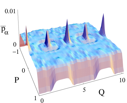
FIG. 8.: Average overlap intensity for a Gaussian wave packet defined in the Birkhoff coordinates of the stadium.

The heights of the bouncing ball peaks can be approximated by quantizing the rectangular region of the stadium. The intensities obtained from this calculation are weighted by the ratio of the density of the bouncing ball states [50] to the total density of states. The Gaussian wave packet is placed in the center of the straight edge and the middle energy regime is used. The results of this approximation are 80.6 and 320.5 for the average intensity and rms intensity, respectively, compared to 80.7 and 386.3 for the numerical calculations of the stadium.

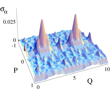
FIG. 9.: Root mean square of the overlap intensity for a Gaussian wave packet defined in the Birkhoff coordinates of the stadium.

Random matrix theory suggests that the correlation coefficient for a generic chaotic system should result in zero. On the other hand, using the correlation coefficient for the stadium in Birkhoff coordinates, we found that some of the states gave nonzero correlations, Fig. (11). In fact, large correlations are found for nearly all the states in the stadium billiard which means that there exists phase space localization for most of the states. The large positive values of the correlation coefficient in the center of the figure again correspond to the bouncing ball states. Classically, this area of phase space is difficult to enter and leave. Hence, the localization is expected to be stronger for this area of phase space. The area beneath the peaks is several standard deviations $(N^{-1/2}=(114)^{-1/2}\approx 0.09)$ away from zero as predicted by random matrix theory. Thus, phase space localization is also occurring in this region. The point exactly in between the peaks is the point in phase space associated with the horizontal bounce. The series of smaller peaks leading up to the large peaks are the gateways into the vertical bouncing ball area. Fig. (12) is a plot of the orbits corresponding to these peaks. They are periodic orbits which only strike the endcaps twice and become almost vertical. Orbits must pass through these regions in order to enter or exit the vertical bounce states.

FIG. 10.: Root mean square of the overlap intensities as a function of $1/\hbar$. The wave packet was placed on the horizontal (solid circles), V (solid squares), diamond (solid triangles), rectangle (open circles) and bow tie (open squares) orbits. The solid line is the theorectial value of $\hbar^{1}$ from Section IV and the dotted line is the best fit of the stadium results which is $\hbar^{1.3}$. The intensities have been rescaled at $\hbar=1$ so that they occupy the same area of the plot.

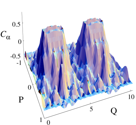
FIG. 11.: Overlap correlation coefficient for the stadium using Birkhoff coordinates. The energy range of the averaging is 2200-2600 where $\hbar=m=1$.

As the energy of the system is increased (i. e. $\hbar$ is decreased), the results of the correlation function remain qualitatively the same, Fig. (13). All the peaks and valleys stay in the same place. The numerical results of the overlap correlation coefficient fluctuate depending upon the area of phase space being considered. This is consistent with the the semiclassical theory in Section IV. More details of the system are explored as $\hbar$ is decreased, since the phase space is divided into finer areas. Thus, more detailed information about the phase space localization of the system is observed in the overlap correlation coefficient at smaller values of $\hbar$.

FIG. 12.: Trajectories corresponding to the peaks leading up to the bouncing ball orbits. The lower figure is a contour plot of Fig. (13). The solid circles correspond to the bounce points of the trajectories. Geometric and time-reversal symmetries were also included.

VI Conclusions

We have shown that intensity weighted level velocities are a good measure of the localization properties for chaotic systems. They are far more sensitive to localization than similarly weighted level curvatures (which are closely related to level statistics). Thus, a system can be RMT-like, yet the eigenstates are not behaving ergodically (as RMT predicts).

The stadium eigenstates show a great deal of localization. Not only are the vertical bouncing ball orbits predicted by the measure, but also other orbits. The overlap correlation coefficient is very parameter dependent. Choosing a different parameter to vary would highlight other sets of orbits depending on how strong the perturbation effects those orbits. The degree of localization can be predicted by the return dynamics. In a chaotic system, all the return dynamics can be organized by the homoclinic orbits. The manner in which a chaotic system’s eigenstates approach ergodicity as $\hbar\rightarrow 0$ will depend on a new time scale, i.e. that required for the homoclinic excursions to explore the available phase space fully.

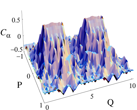
FIG. 13.: The same as Fig. (11) except for a higher energy range of 9200-10000 where $\hbar=m=1$. Note the finer structure of the various peaks.

Parametrically varied data exist that can be analyzed in this way. In the Coulomb-blockade conductance data to the extent that the resonance energy variations are related to a single particle level velocity (minus a constant charging energy and absent residual interaction effects) should show correlations. We mention also that the microwave cavity data can be studied with even more flexibility since they have measured the eigenstates and can therefore meticulously study a wide range of $|\alpha\rangle$ to get a complete picture of the eigenstate localization properties.

Finally, this analysis could be applied in a very fruitful way to near-integrable and mixed phase space systems. In these cases, standard random matrix theory would not give the zero^th order statistical expectation, but the localization would still be determined by the return dynamics in the semiclassical approximation.

A Gaussian Integration

Inserting Eq. (51) into Eq. (49), the strength function involves two $N$-dimensional integrals where $N$ is the system’s number of degrees of freedom,

$$S_{\alpha,osc}(E) = {-1\over\pi}{\mathrm{I}m}{1\over i\hbar(2\pi i\hbar)^{(d-1)/2}}\left({1\over\pi\sigma^{2}}\right)^{d/2}$$ (A4)

$$\times\int\sum_{j}|D_{s}|^{1/2}\exp\{-i{\bf p}_{\alpha}\cdot({\bf q}-{\bf q}^{\prime})/\hbar$$

$$-({\bf q}-{\bf q}_{\alpha})^{2}/2\sigma^{2}-({\bf q}^{\prime}-{\bf q}_{\alpha})^{2}/2\sigma^{2}$$

$$+iS_{j}({\bf q},{\bf q}^{\prime};E)/\hbar-i\nu_{j}^{\prime}\pi/2\}d{\bf q}d{\bf q}^{\prime}$$

To evaluate the integrals over ${\bf q}$ and ${\bf q}^{\prime}$, the action is quadratically expanded about the points ${\bf q}_{f}$ and ${\bf q}_{i}$,

$$S_{j}({\bf q},{\bf q}^{\prime};E) = S_{j}({\bf q}_{f},{\bf q}_{i};E)+{\bf p}_{f}\cdot({\bf q}-{\bf q}_{f})-{\bf p}_{i}\cdot({\bf q}^{\prime}-{\bf q}_{i})$$ (A5)

$$+ {1\over 2}\sum^{N}_{i,k}\left[\left({\partial p^{(i)}_{f}\over\partial q^{(k)}}\right)_{{\bf q}_{f}}(q^{(i)}-q^{(i)}_{f})(q^{(k)}-q^{(k)}_{f})\right.$$ (A6)

$$- \left.\left({\partial p^{(i)}_{i}\over\partial q^{\prime(k)}}\right)_{{\bf q}_{i}}(q^{\prime(i)}-q^{(i)}_{i})(q^{\prime(k)}-q^{(k)}_{i})\right.$$ (A7)

$$+ \left.2\left({\partial p^{(i)}_{f}\over\partial q^{\prime(k)}}\right)_{{\bf q}_{i}}(q^{(i)}-q^{(i)}_{f})(q^{\prime(k)}-q^{(k)}_{i})\right]$$ (A8)

It is useful to define the vector

$${\bf z}=(z_{1},\dots,z_{N},z^{\prime}_{1},\dots,z^{\prime}_{N})$$ (A9)

where

$$z_{i} = (q^{(i)}-q^{(i)}_{f})/\sigma$$ (A10)

$$z^{\prime}_{i} = (q^{\prime(i)}-q^{(i)}_{i})/\sigma$$ (A11)

Thus, the integrals become

$$S_{\alpha,osc}(E) = {-1\over\pi}{\mathrm{I}m}{1\over i\hbar(2\pi i\hbar)^{(d-1)/2}}\left({1\over\pi\sigma^{2}}\right)^{d/2}$$ (A14)

$$\times\int\sum_{j}|D_{s}|^{1/2}\sigma^{2d}$$

$$\times\exp\{-{\bf z}\cdot{\bf A}\cdot{\bf z}-{\bf b}\cdot{\bf z}+c\}d{\bf z}$$

where ${\bf A}$ is composed of four $N$-dimensional matrices

$${\bf A}=\left(\begin{array}[]{cc}{\bf A}^{11}&{\bf A}^{12}\\ {\bf A}^{21}&{\bf A}^{22}\\ \end{array}\right)$$ (A15)

and

$${\bf b} = \left(i\delta p^{(1)}_{f}-\delta q^{(1)}_{f},\dots,i\delta p^{(N)}_{f}-\delta q^{(N)}_{f},\right.$$ (A17)

$$\left.i\delta p^{(1)}_{i}-\delta q^{(1)}_{i},\dots,i\delta p^{(N)}_{i}-\delta q^{(N)}_{i}\right)$$

with

$$\delta p^{(i)}_{f} = (p^{(i)}_{\alpha}-p^{(i)}_{f})\sigma/\hbar$$ (A18)

$$\delta p^{(i)}_{i} = (p^{(i)}_{\alpha}-p^{(i)}_{i})\sigma/\hbar$$ (A19)

$$\delta q^{(i)}_{f} = (q^{(i)}_{\alpha}-q^{(i)}_{f})/\sigma$$ (A20)

$$\delta q^{(i)}_{i} = (q^{(i)}_{\alpha}-q^{(i)}_{i})/\sigma$$ (A21)

and

$$c = {i\over\hbar}S_{j}({\bf q}_{f},{\bf q}_{i};E)-{i\over\hbar}{\bf p}_{\alpha}\cdot({\bf q}_{f}-{\bf q}_{i})$$ (A23)

$$-{({\bf q}_{f}-{\bf q}_{\alpha})^{2}\over 2\sigma^{2}}-{({\bf q}_{i}-{\bf q}_{\alpha})^{2}\over 2\sigma^{2}}-{i\nu_{j}^{\prime}\pi\over 2}$$

The matrix ${\bf A}$ can be expressed in terms of the stability matrix, ${\bf M}$, where ${\bf M}$ has the same form as Eq. (A15)

$$\left(\begin{array}[]{c}{\bf p}\\ {\bf q}\end{array}\right)={\bf M}\left(\begin{array}[]{c}{\bf p}^{\prime}\\ {\bf q}^{\prime}\end{array}\right)$$ (A24)

Thus,

$${\bf A}^{11}_{ab} = {\delta_{a,b}\over 2}-{i\sigma^{2}\over 2\hbar}\left({\partial p^{(a)}_{f}\over\partial q^{(b)}}\right)_{{\bf q}_{f}}$$ (A25)

$$= {\delta_{a,b}\over 2}-{i\sigma^{2}\over 2\hbar}{\sum^{N}_{i}m_{a,i}{\mathrm{c}of}\left({\bf M}^{21}_{b,i}\right)\over\det{\bf M}^{21}}$$ (A26)

$$= {{\bf I}\over 2}-{i\sigma^{2}\over 2\hbar}{\bf M}^{11}({\bf M}^{21})^{-1}$$ (A27)

$${\bf A}^{12}_{ab} = -{i\sigma^{2}\over 2\hbar}\left({\partial p^{(a)}_{f}\over\partial q^{\prime(b)}}\right)_{{\bf q}_{i}}$$ (A28)

$$= {i\sigma^{2}\over 2\hbar}{{\mathrm{c}of}\left({\bf M}^{21}_{b,a}\right)\over\det{\bf M}^{21}}$$ (A29)

$$= {i\sigma^{2}\over 2\hbar}(({\bf M}^{21})^{-1})^{T}$$ (A30)

$${\bf A}^{21}_{ab} = {i\sigma^{2}\over 2\hbar}\left({\partial p^{(a)}_{i}\over\partial q^{(b)}}\right)_{{\bf q}_{f}}$$ (A31)

$$= {i\sigma^{2}\over 2\hbar}{{\mathrm{c}of}\left({\bf M}^{21}_{a,b}\right)\over\det{\bf M}^{21}}$$ (A32)

$$= {i\sigma^{2}\over 2\hbar}({\bf M}^{21})^{-1}$$ (A33)

$${\bf A}^{22}_{ab} = {\delta_{a,b}\over 2}+{i\sigma^{2}\over 2\hbar}\left({\partial p^{(a)}_{i}\over\partial q^{\prime(b)}}\right)_{{\bf q}_{i}}$$ (A34)

$$= {\delta_{a,b}\over 2}-{i\sigma^{2}\over 2\hbar}{\sum^{N}_{i}m_{i+N,b+N}{\mathrm{c}of}\left({\bf M}^{21}_{i,a}\right)\over\det{\bf M}^{21}}$$ (A35)

$$= {{\bf I}\over 2}-{i\sigma^{2}\over 2\hbar}({\bf M}^{21})^{-1}{\bf M}^{22}$$ (A36)

where $m_{i,k}$ are elements of the stability matrix and ${\mathrm{c}of}\left({\bf M}^{21}_{ik}\right)$ is the signed minor of ${\bf M}^{21}_{ik}$. $D_{s}$ is a determinate involving second derivatives of the actions,

$$D_{s}=\left|\begin{array}[]{cc}{\partial^{2}S\over\partial{\bf q}\partial{\bf q}^{\prime}}&{\partial^{2}S\over\partial{\bf q}\partial E}\\ {\partial^{2}S\over\partial E\partial{\bf q}^{\prime}}&{\partial^{2}S\over\partial E^{2}}\\ \end{array}\right| = {1\over|\dot{q}^{(N)}||\dot{q}^{\prime(N)}|}\left|{-\partial^{2}S\over\partial\tilde{\bf q}\partial\tilde{\bf q}^{\prime}}\right|$$ (A39)

$$= {1\over|\dot{q}^{(N)}||\dot{q}^{\prime(N)}|}\left({2\hbar\over i\sigma^{2}}\right)^{(d-1)}$$ (A41)

$$\times\left|\tilde{{\bf A}}^{21}\right|$$

The tildes in the determinants in the above equation are used to exclude the $N$th coordinate. To obtain the above result $q^{(N)}$ and $q^{\prime(N)}$ are chosen to be locally oriented along the trajectory where the dots indicate time derivatives. Since ${\bf A}$ is a symmetric matrix, the result for a general Gaussian integral is used and, hence, the strength function becomes

$$S_{\alpha,osc}(E) = {-1\over\pi}{\mathrm{I}m}{1\over i\hbar(2\pi i\hbar)^{(d-1)/2}}\left({\sigma^{2}\over\pi}\right)^{d/2}\left({2\hbar\over i\sigma^{2}}\right)^{(d-1)/2}$$ (A44)

$$\sum_{j}\left({\pi^{2d}\over\det{\bf A}}\right)^{1/2}\left({1\over|\dot{q}^{(N)}||\dot{q}^{\prime(N)}|}\right)^{1/2}\left|\tilde{{\bf A}}^{21}\right|^{1/2}$$

$$\times\exp\left\{{1\over 4}{\bf b}\cdot{\bf A}^{-1}\cdot{\bf b}+c\right\}$$

$$= {\sigma\over\pi^{1/2}\hbar}{\mathrm{R}e}\sum_{j}\left({\det\tilde{{\bf A}}^{21}\over\det{\bf A}}\right)^{1/2}\left({1\over|\dot{q}^{(N)}||\dot{q}^{\prime(N)}|}\right)^{1/2}$$ (A46)

$$\times\exp\left\{{1\over 4}{\bf b}\cdot{\bf A}^{-1}\cdot{\bf b}+c\right\}$$

where the time derivatives are evaluated at the saddle points.

B Sum Rule for the Strength Function

The determinant of the $(2N\times 2N)$ matrix ${\bf A}$,

$$\det{\bf A}=\det\left(\begin{array}[]{cc}{{\bf I}\over 2}-{i\sigma^{2}\over 2\hbar}{\bf M}^{11}({\bf M}^{21})^{-1}&{i\sigma^{2}\over 2\hbar}(({\bf M}^{21})^{-1})^{T}\\ {i\sigma^{2}\over 2\hbar}({\bf M}^{21})^{-1}&{{\bf I}\over 2}-{i\sigma^{2}\over 2\hbar}({\bf M}^{21})^{-1}{\bf M}^{22}\\ \end{array}\right)$$ (B1)

can be reduced to determinants of $(N\times N)$ matrices by using the relation $(({\bf M}^{21})^{-1})^{T}=-{\bf M}^{12}+{\bf M}^{11}({\bf M}^{21})^{-1}{\bf M}^{22}$ and some row and column manipulations [51], so that

$$\det{\bf A} = \det\left({-i\sigma^{2}\over 4\hbar}\left[{\bf M}^{11}+{\bf M}^{22}\right.\right.$$ (B3)

$$\left.\left.+i\left({\hbar\over\sigma^{2}}{\bf M}^{21}-{\sigma^{2}\over\hbar}{\bf M}^{12}\right)\right]\right)/\det({\bf M}^{21})$$

The coordinates parallel to the trajectory do not mix with the transverse coordinates, since a point on an orbit will remain on that particular orbit. Thus, the $N$th rows and columns of the individual matrices in the above expression are zero except for the $(N,N)$ elements.

It is convenient to re-express the submatrices of the stability matrix in terms of the Lyapunov exponents. Let $\{\lambda_{i}\}$ be the set of Lyapunov exponents whose real part is positive ordered such that $\lambda_{1}>\lambda_{2}>\cdots>\lambda_{N-1}$. The Lyapunov exponents along the parallel coordinate are zero and we will only work with the reduced $(2(N-1)\times 2(N-1))$ stability matrix in what follows. Let ${\bf\Lambda}$ be the diagonal matrix of the eigenvalues of the reduced stability matrix,

$${\bf\Lambda}=\left(\begin{array}[]{cccccc}e^{\lambda_{1}t}&\cdots&0&0&\cdots&0\\ \vdots&&\vdots&\vdots&&\vdots\\ 0&\cdots&e^{\lambda_{N-1}t}&0&\cdots&0\\ 0&\cdots&0&e^{-\lambda_{1}t}&\cdots&0\\ \vdots&&\vdots&\vdots&&\vdots\\ 0&\cdots&0&0&\cdots&e^{-\lambda_{N-1}t}\\ \end{array}\right)$$ (B4)

Thus, by a similarity transform the reduced stability matrix be can written in terms of the Lyapunov exponents, i.e.

$${\bf M}={\bf L}{\bf\Lambda}{\bf L}^{-1}$$ (B5)

Hence, each of the elements of the stability matrix can be written as

$$m_{ij}=\sum_{k}^{N}a_{ij}^{(k)}e^{\lambda_{k}t}+b_{ij}^{(k)}e^{-\lambda_{k}t}$$ (B6)

where $a_{ij}^{(k)}$ and $b_{ij}^{(k)}$ are linear combinations of the elements of the ${\bf L}$ and ${\bf L}^{-1}$ matrices. Because in general chaotic systems $\lambda\gg 0$, the $b_{ij}^{(k)}$’s may be omitted without seriously effecting the above sum. All the determinants including the numerator and denominator of $\det{\bf A}$ as well as $\det\tilde{{\bf A}}^{21}$, thus, will involve products of Eq. (B6). The homoclinic orbits in the sum begin and end at the intersections of the stable and unstable manifolds near the Gaussian centroid. Since neither manifolds may cross themselves, then in the vicinity of the Gaussian centroid the branches of each manifold are nearly parallel to themselves. Thus, to an excellent approximation, the same similarity transformation will diagonalize the stability matrix for each individual orbit, regardless of the period. Consequently, the elements of ${\bf L}$ and ${\bf L}^{-1}$ are period independent.

Connections can be made between the determinants and the Kolmogorov-Sinai entropy. The Kolmogorov-Sinai entropy, $h_{KS}$, of a system can be expressed using Pesin’s Theorem as the sum of the Lyapunov exponents with positive real part,

$$h_{KS}=\sum_{i}^{N-1}\lambda_{i}$$ (B7)

If there is no mixing between the different coordinates, then the individual matrices ${\bf M}^{11}$, ${\bf M}^{12}$, ${\bf M}^{21}$ and ${\bf M}^{22}$ are diagonal. Thus, each matrix element depends only upon one Lyapunov exponent and the determinants are proportional to $\exp(-h_{KS}t)$. This is the case for two dimensional systems where the parallel and perpendicular coordinates in the stability matrix separate as mentioned above. Hence, we have

$$\left|{\det\tilde{{\bf A}}^{21}\over\det{\bf A}}\right|\propto\exp(-h_{KS}t)$$ (B8)

Unlike the periodic orbits, the homoclinic sum is over segments of the orbits. The number of homoclinic points will proliferate exponentially at the same rate as the fixed points in the neighborhood which is proportional to $\exp(h_{T}T)$ where $h_{T}$ is the topological entropy. This is demonstrated by examining the partitioning of the phase space mentioned in Sect. IV B which has exponential growth. The partitioning reflects the symbolic dynamics of the system. The symbolic code uniquely describes each orbit so that amount of code (partitions) cannot grow faster than the number of periodic points, since each code (partition) cannot represent more than one periodic point.

Finally, the sum rule is obtained by setting the topological entropy and Kolmogorov-Sinai entropy equal to each other. Then, for the special case of no mixing in the stability matrix as mentioned above the combination of the amplitudes and the number of orbits yields

$$\sum_{j}\left|{\det\tilde{{\bf A}}^{21}\over\det{\bf A}}\right|\cdots\rightarrow\int dT\cdots$$ (B9)

REFERENCES

- [1] A. Einstein, Verh. Deutsch. Phys. Ges. Berlin 19, 82 (1917); English translation by C. Jaffe, JILA rep. No. 116.
- [2] S. Tomsovic and E. J. Heller, Phys. Rev. Lett. 70, 1405 (1993).
- [3] M. V. Berry, J. Phys. A: Math. Gen. 10, 2083 (1977).
- [4] A. Voros, in Stochastic Behavior in Classical and Quantum Hamiltonian Systems, eds. G. Casati and G. Ford, Lecture Notes in Physics 93, (Springer, Berlin, 1979) p. 326.
- [5] P. O’Connor, J. Gehlen, and E. J. Heller, Phys. Rev. Lett. 58, 1296 (1987).
- [6] S. Hortikar and M. Srednicki, Phys. Rev. Lett. 80, 1646 (1998).
- [7] A. M. Chang, H. U. Baranger, L. N. Pfeiffer, and K. W. West, Phys. Rev. Lett. 73, 2111 (1994); M. R. Haggerty, N. Spellmeyer, D. Kleppner, and J. B. Delos, Phys. Rev. Lett. 81, 1592 (1998); C. M. Marcus, A. J. Rimberg, R. M. Westervelt, P. F. Hopkins, and A. C. Gossard, Phys. Rev. Lett. 69, 506 (1992).
- [8] H. U. Baranger and P. A. Mello, Phys. Rev. Lett. 73, 142 (1994); C. W. J. Beenakker, Rev. Mod. Phys. 69, 731 (1997); A. M. Chang, H. U. Baranger, L. N. Pfeiffer, K. W. West, and T. Y. Chang, Phys. Rev. Lett. 76, 1695 (1996); J. A. Folk, S. R. Patel, S. F. Godijn, A. G. Huibers, S. M. Cronenwett, C. M. Marcus, K. Campman, and A. C. Gossard, Phys. Rev. Lett. 76, 1699 (1996).
- [9] B. D. Simons, P. A. Lee, and B. L. Altshuler, Phys. Rev. Lett. 70, 4122 (1993).
- [10] Y. Alhassid and H. Attias, Phys. Rev. Lett. 74, 4635 (1995).
- [11] M. L. Mehta, Random Matrices, ed., Academic Press, (1991).
- [12] O. Bohigas, M.-J. Giannoni, and C. Schmit, Phys. Rev. Lett. 52, 1 (1984); J. Physique Lett. 45, 1015 (1984).
- [13] A. V. Andreev, O. Agam, B. D. Simons, and B. L. Altshuler, Phys. Rev. Lett. 76, 3947 (1996).
- [14] S. W. McDonald, Ph. D. dissertation, University of California, Berkeley, Lawrence Berkeley Laboratory Report No. LBL-14837 (1983).
- [15] E. J. Heller, Phys. Rev. Lett. 53, 1515 (1984).
- [16] O. Bohigas, S. Tomsovic, and D. Ullmo, Phys. Rep. 223, 43 (1993).
- [17] R. S. McKay and J. D. Meiss, Phys. Rev. A 37, 4702 (1988).
- [18] R. Ketzmerick, G. Petschel, and T. Geisel, Phys. Rev. Lett. 69, 695 (1992).
- [19] S. Fishman, D. R. Grempel, and R. E. Prange, Phys. Rev. A 36, 289 (1987).
- [20] L. Kaplan and E. J. Heller, Ann. Phys. 264, 171 (1998).
- [21] S. Tomsovic and E. J. Heller, Phys. Rev. Lett. 67, 664 (1991); Phys. Rev. E 47, 282 (1993); Physics Today 46 (7), 38 (1993); P. W. O’Connor, S. Tomsovic and E. J. Heller, Physica D 55, 340 (1992).
- [22] S. Tomsovic, Phys. Rev. Lett. 77, 4158 (1996).
- [23] A. Lakshminarayan, N. R. Cerruti and S. Tomsovic, submitted to Phys. Rev. E.
- [24] B. D. Simons, A. Szafer, and B. L. Altshuler, JETP Lett. 57, 277 (1993).
- [25] B. Mehlig and K. Muller, preprint.
- [26] B. D. Simons and B. L. Altshuler, Phys. Rev. B 48, 5422 (1993).
- [27] P. Gaspard, S. A. Rice, H. J. Mikeska and K. Nakamura, Phys. Rev. A 42, 4015 (1990).
- [28] J. Zakrzewski and D. Delande, Phys. Rev. E 47, 1650 (1993).
- [29] F. von Oppen, Phys. Rev. E 51, 2647 (1995); Phys. Rev. Lett. 73, 798 (1994).
- [30] J. Zakrzewski, D. Delande, and M. Kus, Phys. Rev. E 47, 1665 (1993).
- [31] M. Wilkinson, J. Phys. A 22, 2795 (1989).
- [32] E. K. Riedel and F. von Oppen, Phys. Rev. B 47, 15449 (1993).
- [33] A. M. Lane and R. G. Thomas, Rev. Mod. Phys. 30, 257 (1958).
- [34] S. Tomsovic and J. H. Lefebvre, Phys. Rev. Lett. 79, 3629 (1997).
- [35] M. V. Berry and J. P. Keating, J. Phys. A: Math. Gen. 27, 6167 (1994).
- [36] P. Leboeuf and M. Sieber, Phys. Rev. E 60, 3969 (1999).
- [37] A. M. Ozorio de Almeida, Hamiltonian Systems: Chaos and Quantization, Cambridge University Press, (1988).
- [38] J. H. Hannay and A. M. Ozorio de Almeida, J. Phys. A: Math. Gen. 17, 3429 (1984).
- [39] A. M. Ozorio de Almeida, C. H. Lewenkopf and E. R. Mucciolo, Phys. Rev. E 58, 5693 (1998).
- [40] O. Bohigas, M. J. Giannoni, A. M. Ozorio de Almeida and C. Schmit, Nonlinearity 8, 203 (1995).
- [41] J. Goldberg, U. Smilansky, M. V. Berry, W. Scheizer, G. Wunner and G. Zeller, Nonlinearity 4, 1 (1991).
- [42] A. Lakshminarayan, N. R. Cerruti and S. Tomsovic, Phys. Rev. E 60, 3992 (1999).
- [43] B. Eckhardt, S. Fishman, K. Müller and D. Wintgen, Phys. Rev. A 45, 3531 (1992).
- [44] M. V. Berry, Proc. R. Soc. Lond. A 423, 219 (1989).
- [45] E. J. Heller, in Chaos and Quantum Physics, eds. M. J. Giannoni, A. Voros and J. Zinn-Justin (Elsevier, Amsterdam, 1991).
- [46] J. Moser, Commun. Pure and Appl. Math IX, 673 (1956); G. L. da Silva Ritter, A. M. Ozorio de Almeida and R. Douady, Physica D 29, 181 (1987).
- [47] A. M. Ozorio de Almeida, Nonlinearity 2, 519 (1989).
- [48] L. A. Bunimovich, Funct. Anal. Appl. 8, 254 (1974); Commum. Math. Phys. 65, 295 (1979).
- [49] E. B. Bogomolny, Nonlinearity 5, 805 (1992).
- [50] M. Sieber, U. Smilansky, S. C. Creagh and R. G. Littlejohn, J. Phys. A: Math. Gen. 26, 6217 (1993).
- [51] M. C. Gutzwiller, J. Math. Phys. 12, 343 (1971).