Page 0 1.0

Departments of Ecology and Evolutionary Biology and Mathematics, University of Tennessee, Knoxville, TN 37996 USA

phone (865) 974-8136; fax (865) 974-3067; e-mail: sergey@tiem.utk.edu

Using a weak migration and weak mutation approximation, I study the average waiting time to and the average duration of parapatric speciation. The description of reproductive isolation used is based on the classical Dobzhansky model and its recently proposed multilocus generalizations. The dynamics of parapatric speciation is modeled as a biased random walk with absorption performed by the average genetic distance between the residents and immigrants. If a small number of genetic changes is sufficient for complete reproductive isolation, mutation and random genetic drift alone can cause speciation on the time scale of 10-1000 times the inverse of the mutation rate. Even relatively weak selection for local adaptation can dramatically decrease the waiting time to speciation. The duration of parapatric speciation is shorter by orders of magnitude than the waiting time to speciation. For a wide range of parameter values, the duration of speciation is order one over the mutation rate. In general, parapatric speciation is expected to be triggered by changes in the environment.

Keywords: evolution, allopatric speciation, parapatric speciation, mathematical models

1. INTRODUCTION

Parapatric speciation is usually defined as the process of species formation in the presence of some gene flow between diverging populations. From a theoretical point of view, parapatric speciation represents the most general scenario of speciation which includes both allopatric and sympatric speciation as extreme cases (of zero gene flow and a very large gene flow, respectively). The geographic structure of most species, which are usually composed of many local populations experiencing little genetic contact for long periods of time (Avise 2000), fits the one implied in the parapatric speciation scenario. In spite of this, parapatric speciation has received relatively little attention compared to a large number of empirical and theoretical studies devoted to allopatric and sympatric modes (but see Ripley & Beehler 1990; Burger 1995; Friesen & Anderson 1997; Rolán-Alvarez et al. 1997; Frias & Atria 1998; Macnair & Gardner 1998). Traditionally, studies of parapatric speciation emphasized the importance of strong selection for local adaptation in overcoming the homogenizing effects of migration (e.g. Endler 1977; Slatkin 1982). Recently, it has been shown theoretically that rapid parapatric speciation is possible even without selection for local adaptation if there are many loci affecting reproductive isolation and mutation is not too small relative to migration (Gavrilets et al. 1998, 2000a; Gavrilets 1999).

Earlier theoretical studies of speciation mostly concentrated on the accumulation of genetic differences that could eventually lead to complete reproductive isolation. However, within the modeling frameworks previously used complete reproductive isolation was not possible (but see Nei et al. 1983; Wu 1985). Recently new approaches describing the whole process of speciation from origination to completion have been developed and applied to allopatric (Orr 1995; Orr & Orr 1996; Gavrilets & Hastings 1996; Gavrilets & Boake 1998; Gavrilets 1999), parapatric (Gavrilets 1999; Gavrilets et al. 1998, 2000a) and sympatric (e.g. Turner & Burrows 1995; Gavrilets & Boake 1998; van Doorn et al. 1998; Dieckmann & Doebeli 1999) scenarios. Here, I develop a new stochastic approach to modeling speciation as a biased random walk with absorption. I use this framework to find the average waiting time to and the average duration of parapatric speciation. My results provides insights into a number of important evolutionary questions about the role of different factors (such as mutation, migration, random genetic drift, selection for local adaptation, genetic architecture of reproductive isolation) in controlling the time scale of parapatric speciation.

The method for modeling reproductive isolation adapted below is based on the classical Dobzhansky model (Dobzhansky 1937) discussed in detail in a number of recent publications (e.g. Orr 1995; Orr & Orr 1996; Gavrilets & Hastings 1996; Gavrilets 1997). The Dobzhansky model as originally described has two important and somewhat independent features (Orr 1995). First, the Dobzhansky model suggests that in some cases reproductive isolation can be reduced to interactions of “complementary” genes (that is genes that decrease fitness when present simultaneously in an organism). Second, it postulates the existence of a “ridge” of well-fit genotypes that connects two reproductively isolated genotypes in genotype space. This “ridge” makes it possible for a population to evolve from one state to a reproductively isolated state without passing through any maladaptive states (“adaptive valleys”). The original Dobzhansky model was formulated for the two-locus case. The development of multilocus generalizations has proceeded in two directions. A mathematical theory of the build up of incompatible genes leading to hybrid sterility or inviability was developed by Orr (1995; Orr & Orr 1996) who applied it to allopatric speciation. A complementary approach placing the most emphasis on “ridges” rather than on “incompatibilities” was advanced by Gavrilets (1997, 1999; Gavrilets & Gravner 1997; Gavrilets et al. 1998, 2000ab). This approach makes use of a recent discovery that the existence of “ridges” is a general feature of multidimensional adaptive landscapes rather than a property of a specific genetic architecture (Gavrilets & Gravner 1997; Gavrilets 1997, 2000). Here, I will use the “ridges-based” approach assuming that mating and the development of viable and fertile offspring is possible only between the organisms that are not too different over a specific set of loci responsible for reproductive isolation. The adaptive landscape arising in this model is an example of “holey adaptive landscapes” (Gavrilets & Gravner 1997; Gavrilets 1997, 2000) of which the original two-locus two-allele Dobzhansky model is the simplest partial case. My general results are directly applicable to the original Dobzhansky model.

2. MODEL

I consider a finite population of sexual diploid organisms with discrete non-overlapping generations. The population is subject to immigration from another population. For example, one can think of a peripheral population (or an island) receiving immigrants from a central population (or the mainland). All immigrants are homozygous and have a fixed “ancestral” genotype. Mutation supplies new genes in the population some of which may be fixed by random genetic drift and/or selection for local adaptation. Migration brings ancestral genes which, if fixed, will decrease genetic differentiation of the population from its ancestral state.

In this paper, I consider only the loci potentially affecting reproductive isolation. The degree of reproductive isolation depends on the extent of genetic divergence at these loci. Let $d$ be the number of loci at which two individuals differ. I posit that the probability, $w$, that two individuals are able to mate and produce viable and fertile offspring is a non-increasing function of $d$ such that $w(0)=1$ and $w(d)=0$ for all $d>K$ where $K$ is a parameter of the model specifying the genetic architecture of reproductive isolation. This implies that individuals with identical genotypes at the loci under consideration are completely compatible whereas individuals that differ in more than $K$ loci are completely reproductively isolated. A small $K$ means that a small number of genetic changes is sufficient for completely reproductive isolation. A large $K$ means that a significant genetic divergence is necessary for completely reproductive isolation. If $K$ is equal to the overall number of loci, complete reproductive isolation is impossible (neutral case). This simple model is appropriate for a variety of isolating barriers including premating, postmating prezygotic, and postzygotic (Gavrilets et al. 1998, 2000ab, Gavrilets 1999). I will allow the loci responsible for reproductive isolation to have pleiotropic effects on the degree of adaptation to the local environment (Gavrilets 1999; cf. Slatkin 1981; Rice 1984; Rice & Salt 1988). Specifically, I will assume that each new allele potentially has a selective advantage $s$ ($\geq 0$) over the corresponding ancestral allele in the local environment.

I will use a weak mutation and weak migration approximation (e.g. Slatkin 1976, 1981; Lande 1979, 1985; Tachida & Iizuka, 1991; Barton 1993) neglecting within-population variation. Under this approximation the only role of mutation and migration is to introduce new alleles which quickly get fixed or lost. I will assume that the processes of fixation and loss of alleles at different loci are independent. Within this approximation, the relevant dynamic variable is the number of loci, $D_{b}$, at which a typical individual in the population is different from the immigrants. Variable $D_{b}$ is the average genetic distance between residents and immigrants computed over the loci underlying reproductive isolation. The dynamics of speciation will be modeled as a random walk performed by $D_{b}$ on a set of integers $0,1,\dots,K,K+1$. In what follows I will use $\lambda_{i}$ and $\mu_{i}$ for the probabilities that $D_{b}$ changes from $i$ to $i+1$ or $i-1$ in one time step (generation). The former outcome occurs if a new allele supplied by mutation gets fixed in the population. The latter outcome occurs if an ancestral allele brought by immigrants replaces a new allele previously fixed. I disregard the possibility of more than one substitution in one time step. Probabilities $\lambda_{i}$ and $\mu_{i}$ are small and depend on the rate of migration, $m$, the rate of mutation per gamete per generation, $v$, the strength of selection for local adaptation, $s$, and the population size, $N$. Speciation occurs when $d$ hits the (absorbing) boundary $K+1$. If this happens, the population is completely reproductively isolated from the ancestral genotypes. I do not consider the possibility of backward mutation towards an ancestral state. Fixing new alleles at $K+1$ loci completes the process of speciation.

3. RESULTS

I will compute two important characteristics of the speciation process. The first is the average waiting time to speciation, $t_{0}$, defined as the average time to reach the state of complete reproductive isolation ($D_{b}=K+1$) starting at the ancestral state ($D_{b}=0$). In general, during the interval from $t=0$ to the time of speciation the population will repeatedly accumulate a few substitutions only to lose them and return to the ancestral state at $D_{b}=0$. The second characteristic is the average duration of speciation, $T_{0}$, defined as the time that it takes to get from the ancestral state ($D_{b}=0$) to the state of complete reproductive isolation ($D_{b}=K+1$) without returning to the ancestral state. [The duration of speciation is similar to the conditional time that a new allele destined to be fixed segregates before fixation.]

(a) ALLOPATRIC SPECIATION

It is illuminating to start with the case of no immigration (cf. Orr 1985; Orr & Orr 1996; Gavrilets 1999, pp. 6-8). In this case, the process of accumulation of new mutations is irreversible and the average duration of speciation, $T_{0}$, is equal to the average waiting time to speciation, $t_{0}$.

No selection for local adaptation. With no or very little within-population genetic variation the process of accumulation of substitutions leading to reproductive isolation is effectively neutral (cf., Orr 1995; Orr & Orr 1996). The average number of neutral mutations fixed per generation equals the mutation rate $v$ (Kimura 1983). Thus, the average time to fix $K+1$ mutations is

$$t_{0}=\frac{K+1}{v}.$$ (1)

Selection for local adaptation. In a diploid population of size $N$, the number of mutations per generation is $2Nv$. The probability of a mutant allele with a small selective advantage $s$ being fixed is approximately $2s/(1-exp(-4Ns))$ (Kimura 1983). Thus, the average time to fix $K+1$ mutations is

$$t_{0}=\frac{K+1}{v}\ \frac{1-exp(-S)}{S},$$ (2)

where $S=4Ns$. With $S$ increasing from 0 to, say, 10, the time to speciation $t_{0}$ decreases to approximately 1/10 of that in the case of no selection for local adaptation.

(b) PARAPATRIC SPECIATION

With immigration, the dynamics of $D_{b}$ are controlled by two opposing types of forces. Mutation and selection act to increase $D_{b}$ whereas migration acts to decrease $D_{b}$. The appendix presents exact formulae for $t_{0}$ and $T_{0}$ in the case of parapatric speciation. Below I give some simple approximations valid if $\frac{m}{v}\ exp(-S)$ is not too small.

Threshold function of reproductive compatibility. Here, I assume that the function $w(d)$ specifying the probability that two individuals are not reproductively isolated has a threshold form:

$$w(d)=\left\{\begin{array}[]{cc}1&\mbox{for $d\leq K$},\\ 0&\mbox{for $d>K$}.\end{array}\right.$$ (3)

(Gavrilets et al. 1998, 2000ab; Gavrilets 1999, cf. Higgs and Derrida 1992). This function implies that immigrants have absolutely no problems mating with the residents unless the genetic distance $D_{b}$ exceeds $K$. I start with the worst-case scenario for speciation when not only immigrants can easily mate with residents but also selection for local adaptation is absent (cf., Gavrilets et al. 1998, 2000a; Gavrilets 1999).

	Allopatric case	Parapatric case
$K$	($t_{0}=T_{0}$)	$t^{*}_{0}$	$T^{*}_{0}$
$1$	$\frac{2}{v}$	$(2+R)\frac{1}{v}$	$\frac{2+R}{1+R}\ \frac{1}{v}$
$2$	$\frac{3}{v}$	$(3+3R+2R^{2})\frac{1}{v}$	$\frac{3+4R+2R^{2}}{1+R+2R^{2}}\ \frac{1}{v}$
$3$	$\frac{4}{v}$	$(4+6R+8R^{2}+6R^{3})\frac{1}{v}$	$\frac{4+8R+13R^{2}+6R^{3}}{1+R+2R^{2}+6R^{3}}\ \frac{1}{v}$

Table 1: Exact expressions for the average waiting time to speciation, $t^{*}_{0}$, and the average duration of speciation, $T^{*}_{0}$, for small $K$ with no selection for local adaptation and a threshold function of reproductive compatibility. $R=m/v$.

Figure 1: The average waiting time to speciation, $t_{0}^{*}$, and the average duration of speciation, $T_{0}^{*}$. The $x$-axes give the ratio of migration and mutation rates. In Figure (A), the $y$-axis gives the product of $t_{0}^{*}$ and the mutation rate $v$ on the logarithmic scale. In Figure (B), the $y$-axis gives the product of $T_{0}^{*}$ and the mutation rate $v$ on the linear scale. Solid lines correspond to the exact values (found in the Appendix); dashed lines correspond to the approximate equations (5) and (6). In Figure (B), the lines correspond to $K=1,2,4,6,8$, and $10$ (from bottom to top).

No selection for local adaptation. With no selection for local adaptation and neglecting within-population genetic variation, the process of fixation is approximately neutral. The probability of fixation of an allele is equal to its initial frequency. The average frequency of new alleles per generation is approximately the mutation rate $v$. If the immigrants differ from the residents at $D_{b}=i$ loci, there are $i$ loci that can fix ancestral alleles brought by migration. The average frequency of such alleles per generation is $im$. Thus, the probabilities of stochastic transitions increasing and decreasing $D_{b}$ by one are approximately

$$\lambda_{i}=v,\ \mu_{i}=i\ m.$$ (4)

With small $K$, the exact expressions for $t_{0}$ and $T_{0}$ found in the Appendix are relatively compact (see Table 1). With larger $K$, the approximate equations are more illuminating. The average waiting time to speciation is approximately

$$t^{*}_{0}\approx\frac{1}{v}\left(\frac{m}{v}\right)^{K}K!$$ (5)

The average duration of speciation is approximately

$$T^{*}_{0}\approx\frac{1}{v}\left(1+\frac{\Psi(K+1)+\gamma}{m/v}\right),$$ (6)

where $\gamma\approx 0.577$ is Euler’s constant and $\Psi(.)$ is the psi (digamma) function (Gradshteyn & Ryzhik, 1994). [Function $\Psi(K+1)+\gamma$ slowly increases with $K$ and is equal to 1 at $K=1$, to 2.93 at $K=10$ and to 5.19 at $K=100$.] For example, if $m=0.01,v=0.001$ and $K=5$, then the waiting time to speciation is very long: $t^{*}_{0}\approx 1.35\times 10^{10}$ generations, but if speciation does happen, its duration is relatively short: $T^{*}_{0}\approx 1236$ generations. Figure 1 illustrates the dependence of $t^{*}_{0}$ and $T^{*}_{0}$ on model parameters. Notice that $T^{*}_{0}$ is order $1/v$ across a wide range of parameter values.

Figure 2: Effects of selection for local adaptation and of linear function of reproductive compatibility on the waiting time to speciation. (A) The proportion (on the logarithm scale) by which selection for local adaptation decreases $t_{0}$ ($F_{1}=exp(-KS)\ \frac{1-exp(-S)}{S}$; see equation 8). (B) The proportion (on the logarithm scale) by which $t_{0}$ is reduced relative to $t_{0}^{*}$ if the function of reproductive compatibility is linear ($F_{2}=\sqrt{2\pi}\ exp(-K)$; see equation 12).

Selection for local adaptation. Assume that “new” alleles improve adaptation to the local conditions. Let $s$ be the average selective advantage of a new allele over the corresponding ancestral allele. Each generation there are $2Nv$ such alleles supplied by mutation. The probability of fixation of an advantageous allele is approximately $2s/[1-exp(-4Ns)]$. Migration brings approximately $2Nmi$ ancestral alleles at the loci that have previously fixed new alleles. These alleles are deleterious in the new environment. The probability of fixation of a deleterious allele is approximately $2s/[exp(4Ns)-1]$ (Kimura 1983). Thus, the probabilities of stochastic transitions increasing and decreasing $D_{b}$ by one are approximately

$$\lambda_{i}=v\ \frac{4Ns}{1-exp(-4Ns)},\ \mu_{i}=i\ m\ \frac{4Ns}{exp(4Ns)-1}.$$ (7)

The waiting time to speciation is approximately

$$t_{0}\approx t_{0}^{*}\ exp(-KS)\ \frac{1-exp(-S)}{S},$$ (8)

where $t_{0}^{*}$ is given by equation (5). The average duration of speciation is approximately

$$T_{0}\approx\frac{1}{v}\left(1+\frac{\Psi(K+1)+\gamma}{(m/v)e^{-S}}\right)\ \frac{1-exp(-S)}{S}.$$ (9)

For example, if $m=0.01,v=0.001,K=5$ and $S=2$, then $t_{0}\approx 2.74\times 10^{4}$ generations and $T_{0}=2170$ generations. Thus, selection for local adaptation dramatically decreases $t_{0}$ (in the numerical example, by the factor $\approx$ 50,000) and somewhat increases $T_{0}$ relative to the case of speciation driven by mutation and genetic drift. Figure 2A illustrates the effect of selection for local adaptation on $t_{0}$ in more detail.

Linear function of reproductive compatibility. Here, I assume that the probability of no reproductive isolation decreases linearly with genetic distance $d$ from one at $d=0$ to zero at $d=K+1$:

$$w=\left\{\begin{array}[]{cc}1-i/(K+1)&\mbox{for $d\leq K$},\\ 0&\mbox{for $d>K$}.\end{array}\right.$$ (10)

Now, immigrants experience problems in finding compatible mates even when the genetic distance is below $K+1$.

No selection for local adaptation. With no selection for local adaptation, the probabilities of stochastic transitions $\lambda_{i}$ and $\mu_{i}$ are given by equations (4) with $m$ substituted for an “effective” migration rate

$$m_{i}=m\left(1-\frac{i}{K+1}\right).$$ (11)

The waiting time to speciation is approximately

$$t_{0}\approx t_{0}^{*}\ \sqrt{2\pi}\ exp(-K),$$ (12)

where $t_{0}^{*}$ is given by equation (5). The average duration of speciation is approximately

$$T_{0}\approx\frac{1}{v}\left(1+2\ \frac{\Psi(K+1)+\gamma}{m/v}\right).$$ (13)

where $\gamma$ is Euler’s constant and $\Psi(.)$ is the psi (digamma) function. The last equation differs from equation (6) only by the factor 2 inside the parentheses. For example, with the same values of parameters as above $t_{0}\approx 2.36\times 10^{8}$ generations and $T_{0}=1470$ generations. Thus, $t_{0}$ is significantly reduced (by the factor 57) whereas $T_{0}$ is somewhat larger than in the case of threshold function of reproductive compatibility. Figure 2B illustrates the effect of linear function of reproductive compatibility on $t_{0}$ in more detail.

Selection for local adaptation. With selection for local adaptation, the probabilities of stochastic transitions $\lambda_{i}$ and $\mu_{i}$ are given by equations (7) with $m$ substituted for an “effective” migration rate (11). The average time to speciation is approximately

$$t_{0}\approx t_{0}^{*}\ \sqrt{2\pi}\ exp(-K)\ exp(-KS)\ \frac{1-exp(-S)}{S}.$$ (14)

The average duration of speciation $T_{0}$ is given by equation (9) with an additional factor 2 placed in front of the ratio in the parentheses. As before, selection for local adaptation substantially decreases $t_{0}$ and slightly increases $T_{0}$.

4. DISCUSSION

The results presented above allow one to get insights about the time scale of parapatric speciation driven by mutation, random genetic drift and/or selection for local adaptation. I start the discussion of these results by considering the original Dobzhansky model.

(a) Two-locus two-allele Dobzhansky model

Dobzhansky’s original model (Dobzhansky 1937) describes a two-locus two-allele system where a specific pair of alleles is incompatible in the sense that the interaction of these alleles “produces one of the physiological isolating mechanisms” (p. 282). Let us assume that the immigrants have ancestral haplotype ab and that the derived allele B is incompatible with the ancestral allele a (see Figure 4). In this case, the population can evolve to a state reproductively isolated from the ancestral state via a state with haplotype Ab fixed: ${\bf ab\rightarrow Ab\rightarrow AB}$. [Recently Johnson et al. (2000) considered the probability of parapatric speciation driven by mutation in a somewhat similar model. However, their major equation (eq. 13) is heuristic and does not appear to be justified.] Let $\nu$ be the probability of mutation from an ancestral allele (a and b) to the corresponding derived allele (A or B). The average waiting time to and the average duration of parapatric speciation in this system are given by our general equations with $K=1$ and $v=\nu$. Allowing for equal selective advantage $s$ of derived alleles over the ancestral alleles,

$$t_{0}&={\frac{\left(2\,\nu+m{e^{-S}}\right)\left(1-{e^{-S}}\right)}{{\nu}^{2}S}}\approx\frac{m}{\nu^{2}}\ \frac{1-e^{-S}}{S}\ e^{-S},\\ T_{0}=\frac{(2\nu+me^{-S})(1-e^{-S})}{\nu S(\nu+me^{-S})}\approx\frac{1}{\nu}\ \frac{1-e^{-S}}{S},$$ (15a)

where $S=4Ns$ and the approximations are good if $(m/\nu)exp(-S)>>1$. With no selection for local adaptation (that is if $S=0$), $t_{0}\approx m/\nu^{2},T_{0}\approx 1/\nu$.

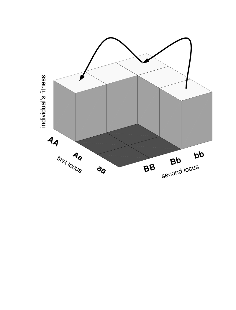
Figure 3: Adaptive landscape in the two-locus two-allele Dobzhansky model. Alleles a and B are incompatible. The arrows specify the chain of gene substitutions leading to complete reproductive isolation.

Let $m=0.01$ and $\nu=10^{-5}$. Then with no selection for local adaptation, the average waiting time to speciation is very long: $t_{0}\approx 10^{8}$ generations, and $T_{0}\approx 10^{5}$ generations. However, even with relatively weak selection for local adaptation, $t_{0}$ can decrease by 1-2 orders of magnitude. For example, with $S=1$, $t_{0}\approx 2.34\times 10^{7},\ T_{0}\approx 6.34\times 10^{4}$; with $S=2$, $t_{0}\approx 5.94\times 10^{6},\ T_{0}\approx 4.36\times 10^{4}$; and with $S=3$, $t_{0}\approx 1.64\times 10^{6},\ T_{0}\approx 3.23\times 10^{4}$. Because the waiting time to speciation in the two-locus Dobzhansky model scales as one over the mutation rate per locus squared, this time is rather long. However, the overall number of loci involved in the initial stages of reproductive isolation is at least on the order of tens to hundreds (e.g. Singh 1990; Wu & Palopoli 1994; Coyne & Orr 1998; Naveira and Masida 1998). This increases the overall mutation rate and can make speciation much more rapid.

(b) Average waiting time to parapatric speciation

In the models studied here, reproductive isolation is a consequence of cumulative genetic divergence over a set of loci potentially affecting mating behavior, fertilization processes, and/or offspring viability and fertility. The underlying biological intuition is that organisms that are reproductively compatible should not be too different genetically. Most species consist of geographically structured populations, some of which experience little genetic contact for long periods of time (Avise 2000). Different mutations are expected to appear first and increase in frequency in different populations necessarily resulting in some geographic differentiation even without any variation in local selection regimes. An interesting question is whether mutation and drift alone are sufficient to result in parapatric speciation. This question is particularly important given a growing amount of data suggesting that rapid evolution of reproductive isolation is possible without selection for local adaptation involved (e.g. Vacquier 1998; Palumbi 1998; Howard 1999). Our results provide an affirmative answer to this question (see also Gavrilets et al. 1998, 2000a; Gavrilets 1999). However, here the waiting time to speciation is relatively short only if a very small number of genetic changes is sufficient for complete reproductive isolation. For example, $t_{0}$ is on the order of 10-1000 times the inverse of the mutation rate if $K=1$ or $2$ with a threshold function of reproductive compatibility, and if $K=1,2$ or $3$ with a linear function of reproductive compatibility. It is well recognized that selection for local adaptation can result in speciation in the presence of some gene flow (e.g. Slatkin 1981; Rice 1984; Rice & Salt 1988; Schluter 1998). Our results show that even relatively weak selection can dramatically reduce the waiting time to speciation by orders of magnitude (see Figure 2a).

(c) How much migration prevents speciation?

In general, evolutionary biologists accept that very small levels of migration are sufficient to prevent any significant genetic differentiation of the populations not to mention speciation (e.g. Slatkin 1987, but see Wade & McCauley 1984). To a large degree, this belief appears to be based on two observations. One is that the expected value of the fixation index $F_{ST}$ is small even with a single migrant per generation (e.g. Hartl & Clark 1997). Another is that the expected distribution of allele frequency in the island model changes from a U-shaped (which implies at least some genetic differentiation) to a bell-shaped (which implies no genetic differentiation on average) as the average number of migrants become larger than one per generation (e.g. Crow & Kimura 1970). However, the equilibrium expectations derived under neutrality theory can be rather misleading if there is a possibility for evolving complete reproductive isolation. For example, in the model with no selection for local adaptation considered above the expected change per generation in the genetic distance $D_{b}$ between the immigrants and residents is

$$\Delta D_{b}=v-mD_{b},$$

where the first term describes an expected increase in $D_{b}$ because of new mutations and the second term describes an expected decrease in $D_{b}$ because of the influx of ancestral genotypes. This equation predicts that $D_{b}$ will reach an equilibrium value of $v/m$. From this one can be tempted to conclude that unless the migration rate is smaller than that of mutation ($v>m$), $D_{b}$ cannot be larger than one and, thus, no speciation is possible. However, this argument is flawed. Because of the inherent stochasticity of the system there is always a non-zero probability of $D_{b}$ moving any pre-specified distance from 0 which will lead to reproductive isolation.

Strictly speaking, in the models studied here migration does not prevent but rather delays speciation. [The resulting delay can be substantial and for all practical reasons infinite.] For definiteness, I will say that speciation is effectively prevented if the average waiting time to speciation is larger than 1000 times the inverse of the mutation rate (that is if $\log_{10}(vt_{0})>3$). If the number of genetic substitutions necessary for speciation is small (for example, $K=1$, as in the original Dobzhansky model, or $K=2$), then migration rates higher than $10v$ will effectively prevent speciation in the absence of selection for local adaptation. For example, if $v=10^{-3}$, then speciation is possible with $m$ as high as 0.01. However, if $v=10^{-5}$, then any migration rate higher than 0.0001 will effectively prevent speciation. If the number of genetic changes required for speciation is relatively large, say, if $K=10$, then without selection for local adaptation speciation is effectively prevented (see Fig. 4a). However, relatively weak selection, say with $S=2.5$ would overcome migration rates as high as $10v$ if the strength of reproductive isolation increases linearly with genetic distance (see Fig.4b).

Within the modeling framework used, all immigrants had a fixed genetic composition which did not change in time. Alternatively, one can imagine two populations exchanging migrants assuming that both populations can evolve. If there is no selection for local adaptation, this case is mathematically equivalent to that studied above but with the mutation rate being twice as large as in the case of a single evolving population. Therefore, the waiting time to speciation in the two population case will dramatically decrease relative to that in the single population case. The maximum migration rates compatible with speciation will be twice as large as before.

Figure 4: Waiting time to speciation with selection for local adaptation for $K=10$. Different lines correspond to $S=0.0,0.5,1.0,1.5,2.0,2.5$, and $3.0$ (from top to bottom). (A) Threshold function of reproductive compatibility (equation 3). (B) Linear function of reproductive compatibility (equation 10).

(c) The role of environment

The waiting time to speciation, $t_{0}$, is extremely sensitive to parameters: changing a parameter by a small factor, say two or three, can increase or decrease $t_{0}$ by several orders of magnitude. Looking across a range of parameter values, $t_{0}$ is either relatively short (if the parameters are right) or effectively infinite. Most of the parameters of the model (such as the migration rate, intensity of selection for local adaptation, the population size, and, probably, the mutation rate) directly depend on the state of the environment (biotic and abiotic) the population experiences. This suggests that speciation can be triggered by changes in the environment (cf. Eldredge 2000). Note that the time lag between an environmental change initiating speciation and an actual attainment of reproductive isolation can be quite substantial as our model shows. If it is an environmental change that initiates speciation, the populations of different species inhabiting the same geographic area should all be affected. In this case, one expects more or less synchronized bursts of speciation in a geographic area - that is a “turnover pulse” (Vrba 1985).

(d) Average duration of parapatric speciation

In our model, the average waiting time to and the average duration of allopatric speciation are identical. Previously, Lande (1985) and Newman et al. (1985) studied how an isolated population can move from one adaptive peak to another by random genetic drift. They showed that the average duration of stochastic transitions between the peaks is much shorter than the time that the population spends in a neighborhood of the initial peak before the transition. Within the framework used by these authors stochastic transitions are possible in a reasonable time only if the adaptive valley separating the peaks is shallow. This implies that reproductive isolation resulting from a single transition is very small. Potentially, strong or even complete reproductive isolation (that is speciation) can result from a series of peak shifts along a chain of “intermediate” adaptive peaks such that each individual transition is across a shallow valley but the cumulative effect of many peak shifts is large (Walsh 1982). In this case, the results of Lande (1985) and Newman et al. (1985) actually imply that the population will spent a very long time at each of the intermediate adaptive peaks. This would lead to a very long duration of allopatric speciation that is in fact comparable to the overall waiting time to speciation.

For parapatric speciation, the predictions are very different. Our results about the duration of speciation lead to three important generalizations. The first is that the average duration of parapatric speciation, $T_{0}$, is much smaller than the average waiting time to speciation, $t_{0}$. This feature of the models studied here is compatible with the patterns observed in the fossil record which form the empirical basis of the theory of punctuated equilibrium (Eldredge 1971; Eldredge & Gould 1972). The second generalization concerns the absolute value of $T_{0}$. The waiting time to speciation changes dramatically with slight changes in parameter values. In contrast, the duration of speciation is on the order of one over the mutation rate over a subset of the loci affecting reproductive isolation for a wide range of migration rates, population sizes, intensities of selection for local adaptation, and the number of genetic changes required for reproductive isolation. Given a “typical” mutation rate on the order of $10^{-5}-10^{-6}$ per locus per generation (e.g. Griffiths et al. 1996; Futuyma 1997) and assuming that there are at least on the order of 10-100 genes involved in the initial stages of the evolution of reproductive isolation (e.g. Singh 1990; Wu & Palopoli 1994; Coyne & Orr 1998; Naveira & Masida 1998), the duration of speciation is predicted to range between $10^{3}$ and $10^{5}$ generations with the average on the order of $10^{4}$ generations. The third generalization is about the likelihood of situations where strong but not complete reproductive isolation between populations is maintained for an extended period of time (much longer than the inverse of the mutation rate) in the presence of small migration without the populations becoming completely isolated or completely compatible. Judging from our theoretical results, such situations appear to be extremely improbable.

(e) Validity of the approximations used

The results presented here are based on a number of approximations the most important of which is the assumption that within-population genetic variation in the loci underlying reproductive isolation can be neglected. A biological scenario to which this assumption is most applicable is that of a small (peripheral) populations with not much genetic variation maintained and with occasional influx of immigrants from the main population. [ Note that within-population genetic variation in the loci underlying reproductive isolation has to be manifested in reproductive incompatibilities between some members of the population. However, the overall proportion of incompatible mating pairs within the population is not expected to be large (e.g. Wills 1977; Nei et al.1983; Gavrilets 1999).] Intuitively, one might expect that increasing within-population variation would substantially increase the rate of substitutions by random genetic drift and make speciation easier. However, in polymorphic populations the alleles affecting the degree of reproductive isolation cannot be treated as neutral because they are weakly selected against than rare (Gavrilets et al. 1998, 2000a; Gavrilets 1999). In the absence of selection for local adaptation this might make speciation somewhat more difficult. Allowing for genetic variation among immigrants can increase the plausibility of speciation. For example, if new alleles are deleterious in the ancestral environment and are maintained there by mutation, their equilibrium frequency will be order $v/s^{*}$, where $s^{*}$ is the selection coefficient against new alleles in the ancestral environment. Thus, the overall frequency of new alleles in the population per generation will increase from $v$ to approximately $v+m\frac{v}{s^{*}}$. Intuitively, this can result in a substantial reduction in the waiting time to speciation. The overall effect of genetic variation (both within-population and among immigrants) on the waiting time to parapatric speciation has to be explored in a systematic way. This is especially important given that the individual-based simulations reported in Gavrilets et al. (1998, 2000a) show that rapid speciation is possible well beyond the domain of parameter values identified here as conducive to speciation. As for the duration of speciation, I expect it to have an order of one over the level of genetic variation maintained in the loci underlying reproductive isolation. As such, with genetic variation the duration of speciation is expected to be (much) shorter than $1/v$.

I am grateful to Janko Gravner for helpful suggestions and to Chris Boake for comments on the manuscript. This work is supported by National Institutes of Health grant GM56693 and by EPPE fund (University of Tennesee, Knoxville).

APPENDIX

Average waiting time till speciation. I consider a Markov chain with $K+1$ states $0,1,\dots,K,K+1$. Let $p_{ij}$ be the corresponding transition probabilities. I assume that the state $K+1$ is absorbing but the state 0 is not. Let $t_{i}$ be the average time till absorption starting from $i$. The mean absorption times satisfy to a general system of linear equations

$$t_{i}=1+\sum_{j}p_{ij}t_{j}$$ (16)

for $i=0,1,\dots,K$ with $t_{K+1}=0$ (e.g. Norris 1997). I assume that the transition probabilities are $p_{i,i+1}=\lambda_{i},p_{i,i-1}=\mu_{i}$ and $p_{ij}=0$ if $|i-j|>1$ with $\mu_{K+1}=0$. In this case, the system of linear equations (16) can be solved by standard methods (e.g. Karlin & Taylor 1975).

Let $z_{i}=t_{i}-t_{i+1}$. From equation (16) with $i=0$ one finds an equality $t_{0}=1+\lambda_{0}t_{1}+(1-\lambda_{0})t_{0}$ which can be rewritten as

$$z_{0}=1/\lambda_{0}.$$ (17a)

In a similar way, for $$i>0 t_{i}=1+\lambda_{i}t_{i+1}+\mu_{i}t_{i-1}+(1-\lambda_{i}-\mu_{i})t_{i}$$ one finds an equality which can be rewritten as

$$z_{i}=\frac{\mu_{i}}{\lambda_{i}}z_{i-1}+\frac{1}{\lambda_{i}}.$$ (17b)

The solution of the system of linear recurrence equations (17) is

$$z_{i}=\frac{\rho_{i}}{\lambda_{0}}+\sum_{j=1}^{i}\frac{\rho_{i}}{\lambda_{j}\rho_{j}},$$ (18a)

where

$$\rho_{j}=\frac{\mu_{1}\mu_{2}\dots\mu_{j}}{\lambda_{1}\lambda_{2}\dots\lambda_{j}}$$ (18b)

with $\rho_{0}=1$. One can also see that $\sum_{i=0}^{K}z_{i}=(t_{0}-t_{1})+(t_{1}-t_{2})+\dots(t_{K}-t_{K+1})=t_{0}$. Thus, $t_{0}$ can be found by summing up equations (18a):

$$t_{0}=\frac{\sum_{i=0}^{K}\rho_{i}}{\lambda_{0}}+\sum_{i=1}^{K}\sum_{j=1}^{i}\frac{\rho_{i}}{\lambda_{j}\rho_{j}}.$$ (19)

The absorption times $t_{i}$ corresponding to $i>0$ can be found recursively using equation (17b).

With a threshold function of reproductive compatibility (3),

$$\rho_{j}=R^{j}j!,$$ (20)

where $R=(m/v)exp(-S)$. With a linear function of reproductive compatibility (10),

$$\rho_{j}=R^{j}j!\ \frac{K!}{(K+1)^{j}(K-j)!}.$$ (21)

Average duration of speciation. The average duration of speciation, $T_{0}$, can be defined as the average time that it takes to walk from state $0$ to state $K+1$ without returning to state $0$. Ewens (1979, Section 2.11) provides formulae that can be used to find $T_{0}$. These formulae are summarized below.

The probability of entering state $K+1$ before state $0$ starting from $i$ is

$$\pi_{i}=\sum_{j=0}^{i-1}\rho_{j}/\ \sum_{j=0}^{K}\rho_{j}.$$ (22)

Starting from state $i$, the mean time spent in state $j$ before entering state $0$ or state $K+1$ is

$$t_{ij}&=(1-\pi_{i})\sum_{k=0}^{j-1}\rho_{k}/(\rho_{j}\lambda_{j})\ {\rm for}\ j=1,\dots,i,\\ t_{ij}=\pi_{i}\sum_{k=j}^{K}\rho_{k}/(\rho_{j}\lambda_{j})\hskip 36.135pt{\rm for}\ j=i+1,\dots,K.$$ (23a)

Starting from state $i$, the conditional mean time spent in state $j$ for those cases for which the state $K+1$ is entered before state $0$ is

$$t^{*}_{ij}=t_{ij}\pi_{j}/\pi_{i}.$$ (24)

The condition mean time till absorption in $K+1$ is

$$t^{*}_{i}=\sum_{j=1}^{K}t^{*}_{ij}.$$ (25)

The average duration of speciation is the sum of the average time spent in state $0$ before moving to state $1$, which is $1/\lambda_{0}$, plus the conditional mean time till absorption in $K+1$ starting from state $1$, which is $t^{*}_{1}$,

$$T_{0}=1/\lambda_{0}+t^{*}_{1}.$$ (26)

REFERENCES

1. Avise, J. C. 2000 Phylogeography. Harvard University Press, Cambridge, Massachusetts.

2. Barton, 1993 The probability of fixation of a favoured allele in a subdivided population. Genet. Res. 62, 149-157.

3. Burger, W. 1995 Montane species-limits in Costa Rica and evidence for local speciation on attitudinal gradients. In Biodiversity and conservation of neotropical montane forests (S. P. Churchill, ed.), pp. 127-133. New York:The New York Botanical Garden.

4. Coyne, J. A. & H. A. Orr. 1998 The evolutionary genetics of speciation. Phil. Trans. R. Soc. Lond. B 353, 287-305.

5. Crow, J. F. & Kimura, M. 1970 An introduction to population genetics theory. Minneapolis, Minnesota: Burgess Publishing Company.

6. Dieckmann, U. & Doebeli, M. 1999 On the origin of species by sympatric speciation. Nature, 400, 354-357.

7. Dobzhansky, Th. G. 1937 Genetics and the origin of species. New York: Columbia University Press.

8. Eldredge, N. 1971 The allopatric model and phylogeny in Paleozoic invertebrates. Evolution 25, 156-167.

9. Eldredge, N. 2000 The sloshing bucket: how the physical realm controls evolution. Pp. 000-000 in Crutchfield, J. and P. Schuster (eds.) Towards a Comprehensive Dynamics of Evolution - Exploring the Interplay of Selection, Neutrality, Accident, and Function. Oxford University Press. (In the press.)

10. Eldredge, N. & Gould, S. J. 1972 Punctuated equilibria: an alternative to phyletic gradualism. In Models in paleobiology (ed. Schopf, T. J.), pp. 82-115. San Francisco: Freeman, Cooper.

11. Endler, J. A. 1977 Geographic variation, speciation and clines. Princeton, NJ: Princeton University Press.

12. Ewens, W. J. 1979 Mathematical population genetics. Berlin: Springer-Verlag.

13. Frias, D. & Atria, J. 1998 Chromosomal variation, macroevolution and possible parapatric speciation in Mepraia spinolai (Porter) (Hemiptera: Reduviidae). Genetics and Molecular Evolution 21, 179-184.

14. Friesen, V. L. & Anderson, D. J. 1997. Phylogeny and evolution of the Sulidae (Aves: Pelecaniformes): a test of alternative modes of speciation. Molecular Phylogenetics and Evolution, 7, 252-260.

15. Futuyma, D. J. 1997 Evolutionary biology. Sunderland, MA: Sinauer.

16. Gavrilets, S. 1997 Evolution and speciation on holey adaptive landscapes. Trends Ecol. Evol. 12, 307-312.

17. Gavrilets, S. 1999 A dynamical theory of speciation on holey adaptive landscapes. Amer. Natur. 154, 1-22.

18. Gavrilets, S. 2000. ”Evolution and speciation in a hyperspace: the roles of neutrality, selection, mutation and random drift.” In Crutchfield, J. and P. Schuster (eds.) Towards a Comprehensive Dynamics of Evolution - Exploring the Interplay of Selection, Neutrality, Accident, and Function. Oxford University Press. (In the press.)

19. Gavrilets, S. & Boake, C. R. B. 1998 On the evolution of premating isolation after a founder event. Amer. Natur. 152, 706-716.

20. Gavrilets, S. & Gravner, J. 1997 Percolation on the fitness hypercube and the evolution of reproductive isolation. J. Theor. Biol. 184, 51-64.

21. Gavrilets, S. & Hastings, A. 1996 Founder effect speciation: a theoretical reassessment. Amer. Nat. 147, 466-491.

22. Gavrilets, S., Li, H. & Vose, M. D. 1998 Rapid parapatric speciation on holey adaptive landscapes. Proc. Roy. Soc. Lond. B 265, 1483-1489.

23. Gavrilets, S., Li, H. & Vose, M. D. 2000a Patterns of parapatric speciation. Evolution 54, 000-000.

24. Gavrilets, S., Acton, R. & Gravner, J. 2000b Dynamics of speciation and diversification in a metapopulation. Evolution 54, 000-000.

25. Gradshteyn, I. S. & Ryzhik, I. M. 1994 Tables of Integrals, Series, and Products. San Diego: Academic Press.

26. Griffiths, A. J. F., Miller, J. H., Suzuki, D. T., Lewontin, R. C. & Gelbart,W. M. 1996 An introduction to genetic analysis. 6th ed. New York: W. H. Freeman.

27. Hartl, D. L. & Clark, A. G. 1997 Principles of population genetics. Sunderland, Massachusetts: Sinauer Associates, .

28. Higgs, P. G. & Derrida, B. 1992 Genetic distance and species formation in evolving populations. J. Mol. Evol. 35, 454-465.

29. Howard, D. J. 1999 Conspecific sperm and pollen precedence and speciation. Annu. Rev. Ecol. Syst. 30, 109-132.

30. Johnson, K. P., Adler, F. R. & Cherry, J. L. 2000. Genetic and phylogenetic consequences of island biogeography. Evolution 54, 387-396.

31. Karlin, S. & Taylor, H. M. 1975 A first course in stochastic processes, second ed. San Diego: Academic Press.

32. Kimura, M. 1983 The neutral theory of molecular evolution . New York : Cambridge University Press.

33. Lande, R. 1979 Effective deme size during long-term evolution estimated from rates of chromosomal rearrangement. Evolution 33, 234-251.

34. Lande, R. 1985 The fixation of chromosomal rearrangements in a subdivided population with local extinction and colonization. Heredity 54, 323-332.

35. Lande, R. 1985 Expected time for random genetic drift of a population between stable phenotypic states. Proc. Natl. Acad. Sci. USA 82, 7641-7645.

36. Macnair, M. R. & Gardner, M. 1998 The evolution of edaphic endemics. Pp. 157-171 in Endless Forms: Species and Speciation (eds Howard, D. J. & Berlocher, S. H.). New York: Oxford University Press.

37. Naveira, H. F. & Masida, X. R. 1998 The genetic of hybrid male sterility in Drosophila. In Endless Forms: Species and Speciation (eds Howard, D. J. & Berlocher, S. H.), pp. 330-338. New York: Oxford University Press.

38. Nei, M., Maruyama, T. & Wu, C.-I. 1983 Models of evolution of reproductive isolation. Genetics 103, 557-579.

39. Newman, C. M., Cohen, J. E. & Kipnis, C. 1985 Neo-Darwinian evolution implies punctuated equilibria. Nature 315, 400-401.

40. Norris, J. R. 1997 Markov Chains. Cambridge: Cambridge University Press.

41. Orr, H. A. 1995 The population genetics of speciation: the evolution of hybrid incompatibilities. Genetics 139, 1803-1813.

42. Orr, H. A. & Orr, L. H. 1996 Waiting for speciation: the effect of population subdivision on the waiting time to speciation. Evolution 50, 1742-1749.

43. Palumbi, S. R. 1998 Species formation and the evolution of gamete recognition loci. In Endless forms: species and speciation. (eds Howard, D.J. & Berlocher, S. H.), pp. 271-278. New York: Oxford University Press.

44. Rice, W. R. 1984 Disruptive selection on habitat preferences and the evolution of reproductive isolation: a simulation study. Evolution 38, 1251-1260.

45. Rice, W. R. & Hostert, E. E. 1993 Laboratory experiments on speciation: what have we learned in 40 years? Evolution 47, 1637-1653.

46. Rice, W. R. & Salt, G. B. 1988 Speciation via disruptive selection on habitat preference: experimental evidence. Amer. Natur. 131, 911-917.

47. Ripley, S. D. & Beehler, B. M. 1990. Patterns of speciation in Indian birds. J. of Biogeography 17, 639-648.

48. Rolán-Alvarez, E., Johannesson, K. & Erlandson, J. 1997. The maintenance of a cline in the marine snail Littorina Saxatilis: the role of home site advantage and hybrid fitness. Evolution 51, 1838-1847.

49. Schluter, D. 1998 Ecological causes of speciation. In Endless forms: species and speciation (eds Howard, D. J. & Berlocher, S. H.), pp. 114-129. New York: Oxford University Press.

50. Singh, R. S. 1990 Patterns of species divergence and genetic theories of speciation. In Population Biology. Ecological and Evolutionary Viewpoints (eds Wöhrmann, K. & Jain, C. K.), pp. 231-265. Berlin: Springer-Verlag.

51. Slatkin, M. 1976 The rate of spread of an advantageous allele in a subdivided population. In Population genetics and ecology. (eds Karlin, S. & Nevo, E.), pp. 767-780. New York: Academic Press.

52. Slatkin, M. 1981 Fixation probabilities and fixation times in a subdivided population. Evolution 35, 477-488.

53. Slatkin, M. 1982 Pleiotropy and parapatric speciation. Evolution 36, 263-270.

54. Slatkin, M. 1987 Gene flow and the geographic structure of natural populations. Science 236, 787-792.

55. Tachida, H. & Iizuka, M. 1991 Fixation probability in spatially varying environments. Genet. Res. 58, 243-251.

56. Turner, G. F. & Burrows, M. T. 1995. A model of sympatric speciation by sexual selection. Proc. R. Soc. Lond. B 260, 287-292.

57. Vacquier, V. D. 1998 Evolution of gamete recognition proteins. Science 281, 1995-1998.

58. van Doorn, G. S. , Noest, A. J. & Hogeweg, P. 1998 Sympatric speciation and extinction driven by environment dependent sexual selection. Proc. R. Soc. Lond. B, 265, 1915-1919.

59. Vrba, E. S. 1985. Environment and evolution: alternative causes of the temporal distribution of evolutionary events. South African Journal of Science 81 229-236.

60. Wade, M. J. & McCauley, D. E. 1984 Group selection: the interaction of local deme size and migration in the differentiation of small populations. Evolution 38, 1047-1058.

61. Walsh, J. B. 1982 Rate of accumulation of reproductive isolation by chromosome rearrangements. Amer. Natur. 120, 510-532.

62. Wills, C. J. 1977 A mechanism for rapid allopatric speciation. Amer. Natur. 111, 603-605.

63. Wu, C-I. 1985 A stochastic simulation study of speciation by sexual selection. Evolution 39, 66-82.

64. Wu, C. -I. & Palopoli, M. F. 1994 Genetics of postmating reproductive isolation in animals. Ann. Rev. Genet. 27, 283-308.