The Poincaré–Lyapounov–Nekhoroshev theorem for involutory systems of vector fields

Abstract We extend the Poincaré-Lyapounov-Nekhoroshev theorem from torus actions and invariant tori to general (non-abelian) involutory systems of vector fields and general invariant manifolds.

Introduction.

The celebrated Poincaré-Lyapounov theorem gives conditions ensuring that a periodic solution of a smooth dynamical system is persistent under small perturbations.

The theorem was extended by Nekhoroshev [1] to the case of quasi-periodic solutions of partially integrable hamiltonian systems. His result is referred to as the Poincaré-Lyapounov-Nekhoroshev (PLN) theorem.

Detailed proofs of Nekhoroshev’s result were provided in [6] from an analytical point of view, and in [17] from a geometrical one (the latter work also contains an extension to non-hamiltonian vector fields). The non-hamiltonian frame was fully considered in [18], where generalization of results concerning bifurcation from periodic solutions to bifurcation from quasiperiodic solutions are also considered.

Further developments include extension to infinite dimensional systems (and existence of breathers) [7], to perturbation of systems with non-compact invariant manifolds [14, 15], and to partially integrable bi-hamiltonian systems [20].

All these results are based on the assumption that the algebra ${\mathcal{G}}$ of vector fields under considerations, hamiltonian or otherwise, is abelian; and correspondingly the invariant manifold $\Lambda$ is a torus ${\bf T}^{k}$ or (in the non-compact case [20]) the product of a torus by a contractible manifold.

After the publication of [17] prof. Duistermaat remarked in a kind letter that, by some arguments based on the geometry of foliations, one should expect an equivalent result to hold also in the non-abelian case. The purpose of this note is precisely to extend the PLN theorem to the case of non-abelian algebras of vector fields, and more generally to involutory systems of vector fields, albeit in a slightly different way.

Some words are maybe in order, before going into mathematical detail, about the physical motivation for such a study and possible physical applications of its results.

The main field of applications for the results obtained here would be that of (differentiable) dynamical systems – i.e. systems of first order ODEs on a smooth manifold. In this framework, one of the considered vector fields would be the dynamical one, while the other ones would be symmetries of the former. It should be recalled, indeed, that for first order (systems of) ODEs, contrary to all other cases, the natural algebraic structure for the set ${\mathcal{G}}$ of vector fields being Lie symmetries of this is not that of a Lie algebra (${\mathcal{G}}$ being infinite dimensional as such [25, 28]) but rather that of a Lie module, ${\mathcal{G}}$ being finite dimensional as such [11, 16]. In geometrical terms, this corresponds to having a finitely generated set of vector fields in involution à la Frobenius.

As detailed below, our results is of interest mainly when the invariant manifold whose persistence is considered has a nontrivial topology. It is well known – and rather obvious – that a symmetry of a vector fields maps solutions with a given topology into solutions with the same topology (we are here referring to the topology of trajectories for the solutions) [11, 16]. The result we give here can also be seen as a generalization of this to the case where the vector fields as well as the symmetries depend on control parameters, and moreover to encompass also the case where the symmetry vector fields also have (at least a set of) trajectories with compact closure: this sets further restrictions on the persistence of the resulting compact invariant manifolds.

Acknowledgements. This work was triggered by the remarks (a rather long time ago) of prof. J.J. Duistermaat on my previous work [17]. I also gratefully acknowledge useful discussions with N.N. Nekhoroshev as well as with D. Bambusi, P. Morando and J. Pejsachowicz.

1 Statement of the problem

In this section we describe the general setting of our problem, i.e. persistence of a ${\mathcal{G}}$-invariant submanifold $\Lambda_{0}$ where ${\mathcal{G}}$ is an involutory system of vector fields.

We will not use the most general setting, but the most physically relevant: we deal with a system of parameter-dependent vector fields on a given manifold ${\mathcal{P}}$ (the phase space), so that ${\mathcal{N}}$ is the direct product of the phase space and a parameter space ${\mathcal{Q}}$ (a discussion of the general case will be given elsewhere).

Let ${\mathcal{P}}$ be a smooth manifold of dimension $p$, and ${\mathcal{G}}=\{X_{1},...,X_{d}\}$ a set of smooth vector fields in ${\mathcal{P}}$, which can depend on external parameters $\varepsilon$, say $\varepsilon\in{\bf R}^{q}$.

We assume $(i)$ that for $\varepsilon=0$ there is a smooth submanifold $\Lambda_{0}\subset{\mathcal{P}}$ which is invariant under ${\mathcal{G}}$, i.e. such that $X_{i}:\Lambda_{0}\to{\rm T}\Lambda_{0}$ for all $i=1,...,d$.

We assume moreover that there is a tubular neighborhood $V$ of $\Lambda_{0}$ such that, for $|\varepsilon|$ small enough, $(ii)$ the vector fields ${\mathcal{G}}$ are in involution – in the Frobenius sense – in $V$, and $(iii)$ span a regular distribution in $V$.

Let us briefly recall what these assumptions mean. The $X_{i}$ are in Frobenius involution if $[X_{i},X_{j}]=\sigma_{ij}^{k}(x)X_{k}$, with $\sigma_{ij}^{k}\in{\mathcal{C}}^{\infty}(V)$ smooth real functions (depending also on the external parameters $\varepsilon$) on $V$.

Also, denote by ${\mathcal{D}}_{x}\subseteq{\rm T}_{x}{\mathcal{P}}$ the distribution associated to ${\mathcal{G}}$ at the point $x\in{\mathcal{P}}$; that is,

$${\mathcal{D}}_{x}\ :=\ \{v\in{\rm T}_{x}{\mathcal{P}}\ :\ v=X|_{x}\,,\,X\in{\mathcal{G}}\}\ .$$

(Note that $S\subseteq V\subset{\mathcal{P}}$ is ${\mathcal{G}}$-invariant if, for all $x\in S$, ${\mathcal{D}}_{x}\subseteq T_{x}S$.) Then ${\mathcal{D}}=\bigcup_{\mathcal{P}}D_{x}$ is the distribution on ${\rm T}P$ associated to ${\mathcal{G}}$; this is regular in $U$ if the subspaces ${\mathcal{D}}_{x}\subseteq{\rm T}_{x}{\mathcal{P}}$ have constant dimension for $x\in V$.

We would like to identify conditions ensuring that $\Lambda_{0}$ is part of a smooth family of ${\mathcal{G}}$-invariant manifolds $\Lambda_{\varepsilon}$, isomorphic to $\Lambda_{0}$.

It will be convenient to consider the product space ${\mathcal{N}}={\mathcal{P}}\times{\bf R}^{q}$, and correspondingly $U=V\times{\mathcal{Q}}$ with ${\mathcal{Q}}$ a suitably small neighborhood of the origin in ${\bf R}^{q}$. Our problem can be studied in $U$. We will also write ${\mathcal{N}}_{c}$ for the intersection of ${\mathcal{N}}$ with the level manifold $\varepsilon=c$; by construction, ${\mathcal{N}}_{c}\simeq{\mathcal{N}}_{0}={\mathcal{P}}$.

2 The fiber bundle construction

We will see $U$ as a fiber bundle $(U,\pi,\Lambda_{0})$ over $\Lambda_{0}$, with contractible fiber. Our problem amounts then to the problem of identifying conditions which ensure the existence of a family of ${\mathcal{G}}$-invariant near-zero sections of this bundle.

We are led to consider a certain (in general, nonlinear) connection $\nabla$ on this bundle, and covariantly constant sections of the bundle under $\nabla$.

We define for any point $x\in\Lambda_{0}$ a local smooth manifold $\Sigma_{x}\subset U$ of dimension $s=n-k$ which is transversal to $\Lambda_{0}$, with $\Sigma_{x}\cap\Lambda_{0}=\{x\}$, so that no two such manifolds intersect, and they define a smooth distribution in $U$ . We also consider linear local manifolds $S_{x}$ tangent to $\Sigma_{x}$ in $x$ (the manifolds $\Sigma_{x}$ and $S_{x}$ are canonically identified by $\nabla$); or to choose $\Sigma_{x}$ to be linear, which is fully legitimate [26].

In this way $U$ is a bundle over $\Lambda_{0}$, and $\Sigma_{x}$ represents the fiber through $x\in\Lambda_{0}$; we denote the corresponding projection as $\pi$, and write the bundle as $(U,\pi,\Lambda_{0})$ with $\pi^{-1}(x)=\Sigma_{x}$.

We can also consider $U_{0}=U\cap{\mathcal{N}}_{0}=V$, and $\sigma_{x}:=\Sigma_{x}\cap U_{0}$; these are smooth manifolds of constant dimension $s=n_{p}-k$ (and codimension $n_{q}$ in $\Sigma_{x}$), and we denote by $s_{x}=S_{x}\cap U_{0}$ the corresponding local linear manifolds. Then $U_{0}$ is also a bundle over $\Lambda_{0}$, and $\sigma_{x}$ represents the fiber through $x\in\Lambda_{0}$; we denote the corresponding projection as $\pi_{0}$, and write the bundle as $(U_{0},\pi_{0},\Lambda_{0})$ with $\pi_{0}^{-1}(x)=\sigma_{x}$.

The distribution ${\mathcal{D}}$ associated to ${\mathcal{G}}$ has constant dimension $r$ in $U$, by hypothesis. Moreover, ${\mathcal{D}}$ is tangent to $\Lambda_{0}$, and thus transversal to $\Sigma_{x}$ in $x$ for all $x\in\Lambda$; this implies that ${\mathcal{D}}$ is also transversal to $\Sigma_{x}$ for all points $u\in\Sigma_{x}$ sufficiently near to $x$. If $U$ has been chosen to be sufficiently small – which we assume from now on – the transversality condition is met for all points in $U$. Note that ${\mathcal{D}}$ defines a canonical identification between the local manifolds $\Sigma_{x}$ and $S_{x}$ defined above.

We assumed moreover that $k=r$, hence ${\mathcal{D}}$ defines a (Frobenius integrable) distribution of horizontal spaces in $U$ and thus a (in general, nonlinear) connection $\nabla$ in $U$ [10, 27]. As this is defined by ${\mathcal{G}}$, it will be referred to as the ${\mathcal{G}}$-connection in $U$.

The problem of existence of smooth ${\mathcal{G}}$-invariant manifolds isomorphic to $\Lambda_{0}$ and near to it is, with this construction, translated into the problem of existence of near-zero ${\mathcal{G}}$-invariant sections for $U$, i.e. of sections of $U$ which are invariant under the ${\mathcal{G}}$-connection $\nabla$.

Note that $\nabla$-invariant sections always exist locally over any chart $A$ in $\Lambda_{0}$, due to Frobenius theorem, since ${\mathcal{G}}$ is an involutory system; thus the nontrivial part of the problem is purely global.

As we deal with a small neighborhood of $\Lambda$ we could – and we will indeed – consider the (transverse) linearization of the $X_{i}$ around $\Lambda_{0}$. Correspondingly, we can consider the (transverse) linearization $\nabla_{0}$ of the connection $\nabla$.

We stress that $\nabla$ is in general a nonlinear connection, acting nonlinearly on sections (this is not a problem, as we are only interested in fixed points under this action), while $\nabla_{0}$ is – by definition – linear and has an associated covariant derivative acting linearly on sections. Finally, we note that, as it follows at once from ${\mathcal{G}}$ being Frobenius integrable, the connections $\nabla$ and $\nabla_{0}$ in $U$ are (locally) flat.

3 Loops, Poincaré-Nekhoroshev map, and monodromy matrices

Let us fix a reference point $x\in\Lambda_{0}$, and a loop $\gamma$ through $x$ in $\Lambda_{0}$. Consider then a point $w\in\pi^{-1}(x)=\Sigma_{x}$; the loop $\gamma$ is lifted by the ${\mathcal{G}}$-connection to a curve ${\widehat{\gamma}}$ in $U$, which defines a map in $\Sigma_{x}$.

We associate in this way a (monodromy) map ${\mathcal{M}}_{\gamma}:\Sigma_{x}\to\Sigma_{x}$ to each loop $\gamma$ in $\Lambda_{0}$. These maps obviously form a group, the holonomy group ${\mathcal{H}}_{x}$ at $x$. When we fix a basis for the homology of $\Lambda$, we will refer to the maps $\{{\mathcal{M}}_{\gamma_{1}},...,{\mathcal{M}}_{\gamma_{r}}\}$ as a set of generators for ${\mathcal{H}}_{x}$.

When we consider only contractible loops, the corresponding subgroup ${\mathcal{H}}^{0}_{x}\subseteq{\mathcal{H}}_{x}$ is the restricted holonomy group at $x$. This is a normal subgroup in ${\mathcal{H}}_{x}$, and ${\mathcal{H}}_{x}/{\mathcal{H}}^{0}_{x}$ is discrete [24]. It follows from our assumption that ${\mathcal{G}}$ is Frobenius integrable (via the Ambrose-Singer theorem [2, 24]) that the restricted holonomy group ${\mathcal{H}}^{0}_{x}$ is trivial, ${\mathcal{H}}^{0}_{x}=\{e\}$.

Now, for $x$ an arbitrary reference point on $\Lambda_{0}$ and $\Sigma_{x}=\pi^{-1}x$, $\nabla$-invariant sections of $U$ correspond to points $w\in\Sigma_{x}$ which are fixed points for all elements of ${\mathcal{H}}_{x}$.

Later on, we will find convenient to focus on the linearization of ${\mathcal{M}}_{\gamma}:\Sigma_{x}\to\Sigma_{x}$ at $x$; this is a linear operator acting in the linear space $V={\rm T}_{x}\Sigma_{x}\simeq{\bf R}^{n-k}$, i.e. a $(n-k)$-dimensional matrix, called the monodromy matrix (at $x$) for the loop $\gamma$. We denote this as $M_{\gamma}$.

In this respect, recall that ${\mathcal{M}}_{\gamma}$ also defines a map ${\mathcal{P}}_{\gamma}:S_{x}\to S_{x}$. This will also be called the Poincaré-Nekhoroshev map for $\gamma$ [17, 18]. If we identify $S_{x}$ with a neighbourhood of the identity in $V$, as can be done via $\nabla$, then $M_{\gamma}$ is exactly the linearization of this map.

Monodromy matrices for all loops through $x$ clearly form a group, called the monodromy group at $x$, and representing the linearization of the holonomy group at $x$. Thus we also refer to this as the linearized holonomy group, and denote it as $h_{x}$. Given a set of generators for ${\mathcal{H}}_{x}$, the corresponding linearized operators will be a set of generators for $h_{x}$.

Remark 1. As well known, monodromy groups based at different points are conjugated, and homotopic loops based at the same point provide the same monodromy maps and matrices.

4 The difference Poincaré-Nekhoroshev map and its linearization

We have introduced the Poincaré-Nekhoroshev map ${\mathcal{P}}_{\gamma}:S_{x}\to S_{x}$, and its linearization around $\Lambda$, i.e. the monodromy matrix $M_{\gamma}:V\to V$. By definition, ${\mathcal{P}}_{\gamma}x=x$; at the linear level, $x$ corresponds to the origin in $V$, and $M_{\gamma}0=0$ by linearity. Invariant near-zero sections are obtained for the near-zero $\xi\in V$ such that $M_{\gamma}\xi=\xi$ for all loops $\gamma$.

Instead of considering ${\mathcal{P}}_{\gamma}$ and $M_{\gamma}$, it is more convenient (as in the abelian case) to consider the map ${\mathcal{R}}_{\gamma}:=I-{\mathcal{P}}_{\gamma}:S_{x}\to S_{x}$ and its linearization (also called the linearized difference Poincaré-Nekhoroshev map) $R_{\gamma}=I-M_{\gamma}$; note $R_{\gamma}:V\to V$.

Let us now focus on a given $x\in\Lambda_{0}$ and a given loop $\gamma\subset\Lambda_{0}$ through $x$, and look for $\xi\in\Sigma_{x}$ such that ${\mathcal{R}}_{\gamma}\xi=0$. By definition, $\xi=x$ satisfies this, and we are interested in knowing if there is any nearby $\xi$ satisfying this equation.

This leads to investigate the question of existence of any zero eigenvalue for the linear map $R_{\gamma}$: if this is the case, the zero eigenspace corresponds to fixed points of ${\mathcal{R}}_{\gamma}$ via the implicit function theorem, see below; we stress the implicit function theorem requires a nondegeneracy condition on the map.

If the nondegeneracy conditions are satisfied and there is a common zero eigenvalue of $R_{\gamma}$ for all $\gamma$ through $x$ (zero eigenvalues of $R_{\gamma}$ correspond to unit eigenvalues of $M_{\gamma}$), this corresponds to the required near-zero invariant sections, and hence to invariant manifolds $\Lambda_{\varepsilon}$ isomorphic and $\varepsilon$-close to $\Lambda_{0}$.

Let us make more precise the relation between zeroes of ${\mathcal{R}}_{\gamma}$ near the trivial zero $x$ and the zero eigenspace of $R_{\gamma}$, for a fixed $\gamma$. The following lemma follows at once from the implicit function theorem.

Lemma. Let ${\mathcal{R}}_{\gamma}$ and $R_{\gamma}$ be as above; write $V={\rm T}_{x}\Sigma_{x}\simeq S_{x}\simeq{\bf R}^{n-k}$. Denote the kernel of $R_{\gamma}$ as $K\subseteq V$. Assume there is an invariant complementary space ${\mathcal{T}}$. Then if $K\simeq{\bf R}^{m}$, there is a $m$-dimensional manifold ${\mathcal{K}}\subset\Sigma_{x}$ of zeroes for ${\mathcal{R}}_{\gamma}$, and ${\rm T}_{x}{\mathcal{K}}=K$; for $\varepsilon$ sufficiently small, all zeroes of ${\mathcal{R}}_{\gamma}$ within $\varepsilon$ from the trivial zero $x$ lie on ${\mathcal{K}}$.

Remark 2. Given any loop $\gamma$ through $x$, there is a loop $\gamma^{\prime}$ which is (homotopic to the one) obtained by going $k$ times round $\gamma$; this means that $h_{x}$ will include both $M_{\gamma}$ and all of its powers. If $\mu$ is an eigenvalue of $M_{\gamma}$, there will be an eigenvalue $\mu^{k}$ of $M_{\gamma^{\prime}}$; in particular the presence of an eigenvalue $\mu=e^{i\theta}$ of unit modulus in the spectrum of $M_{\gamma}$ implies that there will be maps $M_{\gamma^{\prime}}=(M_{\gamma})^{k}\in h_{x}$ with an eigenvalue $\mu^{\prime}=e^{ik\theta}$. If $\theta/2\pi$ is rational, there is $k$ such that $\mu^{\prime}=1$: thus we will have actually to require that $\mu\not=\exp(i2\pi m/n)$ for all $m,n\in{\bf Z}$. It should be stressed that if $\theta/2\pi$ is irrational there will however be $k,k^{\prime}$ such that $|k\theta-2k^{\prime}\pi|<\delta$, i.e. $|e^{ik\theta}-1|<\delta$, for any $\delta>0$. This means that in many contexts – in particular when discussing bifurcations [18] – we should also require that all eigenvalues satisfy $|\mu_{i}|\not=1$ (see e.g. [5] for further detail). $\odot$

The maps ${\mathcal{M}}_{\gamma}$ leave $U_{\varepsilon}$ invariant; hence there are matrices $M_{\gamma}^{(0)}$ and $M_{\gamma}^{(1)}$ such that

$$M_{\gamma}=\pmatrix{M_{\gamma}^{(0)}&M_{\gamma}^{(1)}\cr 0&I\cr}\ ;\ \ R_{\gamma}\ =\ \pmatrix{I-M_{\gamma}^{(0)}&-M_{\gamma}^{(1)}\cr 0&0\cr}\ .$$

We denote as $R_{\gamma}^{0}$ the restriction of the map $R_{\gamma}$ to $V_{0}$. By the above formula,

$$R_{\gamma}^{0}\ :=\ I-M_{\gamma}^{(0)}\ .$$

In this case it is immediate to see that the kernel of $R_{\gamma}$ is provided by

$$y\ =\ (R_{\gamma}^{0})^{-1}\,M_{\gamma}^{(1)}\,z\ ,$$

provided the inverse $(R_{\gamma}^{0})^{-1}$ exists (this, of course, is the same nondegeneracy condition which allowed to use the implicit function theorem). The condition for this is just that the spectrum of $M_{\gamma}^{(0)}$ does not include one, i.e. that all the restricted characteristic multipliers (exponents) satisfy $\mu_{i}\not=1$ ($\beta_{i}\not=0$). Note that this must hold for all $\gamma$ (see also Remark 2 below).

Note also that if $M^{(1)}_{\gamma}=0$, we are reduced to the invariant manifold $\Lambda_{0}$ itself, for all values of $z$.

It should be stressed that in general, formula (3) will give different $y$ for the same $z$ when we consider different nonhomotopic loops $\gamma$ (a relevant exception is provided by the case where $h_{x}$ is abelian).

Thus, at difference with the abelian case, we expect that the condition on spectra of monodromy matrices will not suffice to ensure the persistence of invariant manifolds; instead, they will have to be complemented by a ”compatibility condition” ensuring that solutions to (3) for different loops coincide.

On the other hand, if there exists an invariant manifold $\Lambda^{\prime}$, intersecting $S_{x}$ at $\Lambda_{x}^{\prime}=\xi$, the point $\xi$ is a fixed point for $M_{\gamma}$ for any loop $\gamma$ through $x$; thus, if $x\in\gamma\cap\gamma^{\prime}$, the commutator $[M_{\gamma},M_{\gamma^{\prime}}]$ must vanish when applied to $\xi\in S_{x}$: the $\xi(y,z)$ identifying invariant manifolds must belong to ${\rm Ker}([h_{x},h_{x}])\subset V$.

A possible approach, employed in example II below, to discussing if solutions to (3) for different loops $\gamma$ are compatible is as follows.

Subdivide $\Lambda_{0}$ as the union of regions $B_{i}$, $i=1,...h$, each of them with homotopy group $\pi_{1}(B_{i})={\bf Z}$; and denote by $\eta_{i}$ a homotopically nontrivial loop in $B_{i}$, so that the homology of $B_{i}$ is generated by $\eta_{i}$. We also write $M_{i}$ for $M_{\eta_{i}}$, $R_{i}$ for $R_{\eta_{i}}$, and so on.

Consider then (3) for $\gamma=\eta_{i}$: provided $R_{i}^{0}$ is invertible this identifies, for a given value of $z$, an invariant manifold $\Lambda_{i}$ over each of the $B_{i}$.

A necessary condition for the existence of an invariant manifold $\Lambda_{\varepsilon}$ is then that $\Lambda_{i}=\Lambda_{j}$ over $B_{i}\cap B_{j}$, i.e. that the invariant manifolds determined in this way by $\eta_{i}$ and $\eta_{j}$ do coincide over the intersection of the charts $B_{i}$ and $B_{j}$.

If this condition is satisfied over all the nonempty intersection regions $B_{i}\cap B_{j}$, thus determining a possibly invariant manifold ${\widehat{\Lambda}}(z)$, we should still check this is invariant under the other generators of the full homology of $\Lambda_{0}$, i.e. under the monodromy maps for loops $\gamma$ which are not homotopic to a combination of the $\eta_{i}$ for $i=1,...,h$.

5 The PLN theorem for involutory systems of vector fields

We have now completed the geometric construction needed for the Poincaré-Lyapounov-Nekhoroshev theorem in the general case, i.e. for involutory systems of vector fields ${\mathcal{G}}$ which are not necessarily a Lie algebra, nor necessarily abelian.

We took care to provide definitions and introduce notations such to have a statement which looks quite similar to the original one by Nekhoroshev [1, 17] and a proof (actually, constituted to a large extent of the discussion conducted so far) quite similar to the one for the abelian case [17].

Theorem 1. Let ${\mathcal{N}}$, ${\mathcal{G}}$ and ${\mathcal{D}}$ be as in section 2 above. Let $\Lambda_{0}$ and $U$ be as in sections 2 and 3, with $\Lambda_{0}$ compact, connected and $k$-dimensional, and ${\mathcal{D}}$ regular and of dimension $k$ in ${\rm T}U$. Assume moreover that $U$ is foliated into ${\mathcal{G}}$-invariant manifolds $U_{\varepsilon}\simeq{\mathcal{P}}$ of dimension $n_{p}$, with $k<n_{p}<n$, with $\Lambda_{0}\subset U_{0}$, and $U_{\varepsilon}$ transversal to $\pi^{-1}(x)$, so that $V$ admits the decomposition $V=V^{(0)}\oplus V^{(1)}$, and the monodromy matrices can be written in the form (1). Let $\eta_{1},...,\eta_{h}$ be cycles generating the homology of $\Lambda_{0}$, and ${\mathcal{M}}_{j}={\mathcal{M}}_{\eta_{j}}$ the associated monodromy maps; $M_{j}=M_{\eta_{j}}$ the associated monodromy matrices, with $M_{j}^{(0)}$ their restriction to the space $V^{(0)}$.

Then the following are equivalent:

(i) There is a ${\mathcal{G}}$-invariant manifold $\Lambda_{\varepsilon}\subset U_{\varepsilon}$, isomorphic to $\Lambda_{0}$ and $|\varepsilon|$-near to $\Lambda$, for any $\varepsilon$ with $|\varepsilon|<\varepsilon^{*}$;

(ii) (a) If the loops $\eta_{i}$ and $\eta_{j}$ intersect in some point, the commutator $[M_{i},M_{j}]$ has a nontrivial kernel in $V_{x}\simeq{\rm T}_{x}\Sigma_{x}$; (b) The spectrum of any product of the matrices $M^{(0)}_{j}$ associated to loops $\eta_{j}$ such that ${\mathcal{M}}_{j}$ is not the identity does not include points on the unit circle $S^{1}\in{\bf R}^{2}\simeq{\bf C}$, for all $j=1,..,h$.

Proof. It is quite clear that going around loops such that the associated full monodromy map reduces to the identity will have no effect on any consideration to follow (which justifies the specification given in point (ii)-b above), so we can assume all loops we consider have ${\mathcal{M}}\not=I$. By the Ambrose-Singer theorem, this excludes in particular trivial (i.e. contractible) loops.

Let us first consider loops $\gamma$ given by $\eta_{j}\circ...\circ\eta_{j}=\eta_{j}^{m}$ for some loop $\eta_{j}$. In this case the monodromy matrix is

$$M_{\gamma}\ =\ \pmatrix{[M_{j}^{(0)}]^{m}&Z(j,m)\cr 0&I\cr}$$

with $Z(j,m)$ a matrix whose explicit expression (which could be given in terms of $M_{j}^{(0)}$ and $M_{j}^{(1)}$) is not relevant here. Thus

$$R_{\gamma}\ =\ \pmatrix{I-[M_{j}^{(0)}]^{m}&-Z(j,m)\cr 0&0\cr}\ :=\ \pmatrix{R_{j}^{(0)}&-Z(j,m)\cr 0&0\cr}\ .$$

The fixed points under $\gamma$ will be the kernel of this, i.e. – with the notation used in section 4 – will be given by

$$y\ =\ [R_{j}^{(0)}]^{-1}\,Z(j,m)\ z\ .$$

In order for $[R_{j}^{(0)}]^{-1}$ to exist for all $m$, we must require that eigenvalues of $M_{j}^{(0)}$ are bounded away from the unit circle, so that the condition given in the statement is surely necessary for the existence of $\Lambda_{\varepsilon}$.

Let us now consider more general loops $\gamma$. Any loop $\gamma_{0}$ is homotopic (suitably choosing the base point, see also Remark 1) to a loop $\gamma$ which can be written as

$$\gamma\ =\ \eta_{j_{1}}\circ\ ...\ \circ\eta_{j_{\nu}}$$

for some sequence of $\nu\in(1,...,n)$. The associated monodromy matrix is

$$M_{\gamma}\ =\ \pmatrix{M_{j_{1}}^{(0)}...M_{j_{\nu}}^{(0)}&\beta\cr 0&I\cr}\ =\ \pmatrix{\alpha&\beta\cr 0&I\cr}$$

with $\beta$ a complicate expression we do not need to write explicitly.

As usual, we look at the matrix $R_{\gamma}=I-M_{\gamma}$, and we are concerned with the invertibility of $R_{\gamma}^{(0)}$, which is now given by $R_{\gamma}^{(0)}:=I-\alpha$. Thus, in order to have an invariant manifold we have to require that the spectrum of $\alpha$ does not contain the unity. This is precisely (ii)-b.

Finally, note that we need invariant manifolds associated to different loops going through the same point do coincide; this is precisely (ii)-a, and the proof is complete. $\diamondsuit$

Corollary 1. Under the assumptions and with the notation of theorem 1 above, assume moreover that the ${\mathcal{G}}$-invariant manifold $\Lambda_{0}$ has trivial homotopy group, $\pi_{1}(\Lambda_{0})=I$. Then there is $\varepsilon^{*}>0$ such that in the tubular neighborhood of $\Lambda_{0}$ of radius $\varepsilon^{*}$ there is a ${\mathcal{G}}$-invariant manifold $\Lambda$, foliated into ${\mathcal{G}}$-invariant manifolds $\Lambda_{\varepsilon}$ isomorphic to $\Lambda_{0}$.

Proof. If $\pi_{1}(\Lambda)=\{e\}$, all loops $\gamma$ in $\Lambda$ are contractible; hence ${\mathcal{H}}_{x}$ reduce to ${\mathcal{H}}^{0}_{x}$. From the Frobenius integrability of the distribution ${\mathcal{G}}$ it follows that $\nabla$ is flat, and the Ambrose-Singer theorem [2, 24] guarantees that ${\mathcal{H}}=I$. $\diamondsuit$

Let us present some short remarks on the results obtained above.

1. It might be appropriate to stress that in theorem 1 the condition (ii)-b on the spectrum of monodromy matrices is (once (ii)-a is granted) sufficient but not necessary to guarantee the existence of a continuous family of ${\mathcal{G}}$-invariant manifolds, i.e. (i). To see this, just think of the case where the monodromy operators of all loops $\gamma$ are just ${\mathcal{M}}_{\gamma}=I$.

2. We note that when $\Lambda_{0}$ is of codimension one in $U_{0}$ (e.g., if it is of codimension one in phase space), $M^{(0)}_{\gamma}$ are just numbers, and it is very easy to check the conditions given in theorem 1. Similarly, if it happens that the $M_{\eta_{j}}^{(0)}$ commute (albeit the full $M_{\eta_{j}}$ may not commute) it is easy to check that condition.

3. Note that if $\Lambda_{0}$ is the topological product $\Lambda_{0}={\widehat{\Lambda}}_{0}\times B$ of a topologically nontrivial manifold ${\widehat{\Lambda}}_{0}$ and a contractible manifold $B$, then by lemma 3 it suffices to consider ${\widehat{\Lambda}}_{0}$ (as it also follows from the role of homology groups in our discussion). If $\Lambda_{0}$ is contractible, then our result is trivial.

4. It should be stressed that our discussion encompasses cases where – by topological reasons – any vector field on $\Lambda_{0}$ necessarily has fixed points, so that the considered invariant manifold is necessarily not minimal. By a naive parallel with the torus case one could think that in this case the invariant manifold breaks down under perturbations, but actually the same topological constraints guarantees its persistence. In a way, only degenerations which are not enforced by topology are dangerous for persistence.

5. Finally, we note that the abstract results obtained here are qualitatively equivalent to those holding for tori and commuting vector fields [1, 6, 17, 18]; but now checking that the hypotheses hold in concrete situations will in general be quite more difficult than in the abelian case.

6 The coordinate picture

We have so far conducted our discussion in rather abstract terms, in order to make clear the geometric content of our result. However, in order to use it in concrete situations it is convenient to have a formulation in local coordinates as well; this is the aim of the present section.

We will now introduce local coordinates in $U$ and in $U_{0}$. Consider a local chart $B_{i}\subset\Lambda_{0}$ with local coordinates $\varphi$; we naturally associate to this a chart $A_{i}=\pi^{-1}(B_{i})$ in $U$. The natural local coordinates for this will be $(\varphi,w)$ where $\varphi$ are local coordinates in $B_{i}$, and $w=(w^{1},...,w^{S})$ are coordinates on the fiber $\pi^{-1}[x(\varphi)]$.

It is convenient to choose these as $w=(y,z)$ where $y=(y^{1},...,y^{p-k})$ are coordinates in $\sigma_{x}$ and $z=(z^{1},...,z^{a})$ are coordinates in the parameter space ${\mathcal{Q}}$. (For ease of later notation, we choose coordinates $(y,z)$ on $\Sigma_{x}$ such that $|y^{i}|,|z^{a}|\leq\delta$.)

The vector fields $X_{a}$ generating ${\mathcal{G}}$ will be written in these coordinates as

$$X_{a}\ =\ \beta_{a}^{i}{\partial\over\partial\varphi^{i}}\ +\ f_{a}^{k}{\partial\over\partial w^{k}}\ .$$

The linearized connection will be generated by the linearizations of the $X_{a}$ around $\Lambda$; this amounts to replacing $\beta^{i}_{a}$ and $f^{k}_{a}$ by their linearization at $\Lambda$:

$$\begin{array}[]{rl}X_{a}^{0}\ =&\ \left[\beta_{a}^{i}(\varphi,0)+\left({\partial\beta_{a}^{i}\over\partial w^{s}}(\varphi,0)\right)w^{s}\right]\,{\partial\over\partial\varphi^{i}}\ +\\ &\ +\ \left[f_{a}^{k}(\varphi,0)+\left({\partial f_{a}^{k}\over\partial w^{s}}(\varphi,0)\right)w^{s}\right]\,{\partial\over\partial w^{k}}\ .\end{array}$$

As stressed above, we can just consider the action of the linearized holonomy group at $x$, made of $M_{\gamma}$ for all loops $\gamma$ in $\Lambda_{0}$. Its explicit construction is quite standard, but we discuss it briefly below in order to fix notation.

The nonlinear connection $\nabla$ provides a lift of the ordinary derivative $\partial_{\varphi}$ along $\gamma$, which is in general a nonlinear operator (and thus not a proper covariant derivative). This is written in the $(\varphi,w)$ coordinates as

$$\nabla_{\varphi}\ =\ \partial_{\varphi}+A^{i}(\varphi,w){\partial\over\partial w^{i}}\ ,$$

where $A^{i}:\Gamma\to{\bf R}$ is in general a nonlinear function of $w$; as $\Lambda_{0}$ is ${\mathcal{G}}$-invariant, it must be $A^{i}(\varphi,0)=0$. Linearizing around $\gamma$ we have a covariant derivative

$$D_{\varphi}\ =\ {\partial\over\partial\varphi}\ +\ (L^{i}_{j}w^{j}){\partial\over\partial w^{i}}$$

where the matrix $L$, given by $L^{i}_{j}:=(\partial A^{i}/\partial w^{j})(\varphi,0)$, is a function of $\varphi$ alone. The evolution of ${\widehat{\gamma}}(t)=(\varphi(t),w(t))$ along the loop coordinate $t$, i.e. along $\varphi=\varphi_{0}+2\pi t$ is described by ${\dot{\varphi}}=2\pi$, ${\dot{w}}=Lw$; needless to say, the solution to these is

$$\varphi(t)=\varphi_{0}+2\pi t\ \ ;\ \ w(t)=\exp\left[\int_{0}^{t}L[\varphi(\tau)]{\rm d}\tau\right]\ w_{0}\ .$$

The function $\varphi(t)$ is (as obvious by construction) periodic of period one; as $L=L(\varphi)$, the matrix $L$ is also $t$-periodic of period one, and we are thus considering a time-periodic vector equation for the vector variable $w(t)\in{\bf R}^{n-k}$. We can then invoke Floquet theorem (see e.g. [21, 26, 30]).

Proposition. (Floquet theorem) The fundamental solution matrix $\Psi(t)$ for ${\dot{\xi}}=L(t)\xi$ with $L$ a matrix $T$-periodic in $t$ can be written as $\Psi(t)=P(t)\exp[Bt]$ with $P(t)$ a $T$-periodic matrix, and $B$ a constant matrix. In particular, $\Psi(t+T)=\Psi(t)M$, with $M=\exp[BT]$.

The matrix $M$ in the statement above is precisely the monodromy matrix for the given loop $\gamma\subset\Lambda$. The eigenvalues $\mu_{1},...,\mu_{n-k}$ of $M$ are the characteristic (or Floquet) multipliers; if $\nu_{i}$ are the eigenvalues of $B$ we have $\mu_{i}=e^{\nu_{i}T}$, and the $\nu_{i}=\log(\mu_{i}T)$ are the characteristic (or Floquet) exponents.

The information provided by the spectrum of $M$ is best used by passing to coordinates $\eta$ via $\xi=P(t)\eta$; in these the evolution equations read ${\dot{\eta}}=B\eta$, so that $\eta(t)=e^{Bt}\eta_{0}$ and of course $\eta(T)=M\eta_{0}$.

It is worth stressing that the unit vector field $Y$ tangent to ${\widehat{\gamma}}(t)$ in $t$ can always be written in the form $Y=\alpha_{i}(t)X_{i}$, but in general it is not possible to find a $\gamma^{\prime}\simeq\gamma$ such that one can choose the $\alpha_{i}(t)$ as constant, contrary to the abelian case. (However the loop $\gamma$ can be deformed into a piecewise smooth path $\gamma^{\prime}$ homotopic to $\gamma$ on which the $\alpha_{i}(t)$ are piecewise constant.) Thus in the case where ${\mathcal{G}}$ is a Lie algebra, $Y$ does not belong to the algebra ${\mathcal{G}}$, but to the module over ${\mathcal{C}}^{\infty}(\gamma^{\prime})$ generated by ${\mathcal{G}}$. In the terminology of field theory, we should consider the gauge algebra modelled on ${\mathcal{G}}$.

With the notation introduced earlier on in this section, we will write

$$\nabla_{\varphi}\ =\ \partial_{\varphi}+f^{i}(\varphi,y,z){\partial\over\partial y^{i}}+h^{a}(\varphi,y,z){\partial\over\partial z^{a}}\ .$$

The ${\mathcal{G}}$-invariance of $\Lambda_{0}$ entails that $f^{i}(\varphi,0,0)=h^{a}(\varphi,0,0)=0$. Linearizing around $\gamma$ we get

$$D_{\varphi}\ =\ {\partial\over\partial\varphi}\ +\ (F^{i}_{j}y^{j}+G^{i}_{a}z^{a}){\partial\over\partial y^{i}}\ +\ (H^{a}_{j}y^{j}+K^{a}_{b}z^{b}){\partial\over\partial z^{a}}$$

where the matrices $F,G,H,K$ are functions of $\varphi$ alone, and of course we have defined these by $F^{i}_{j}(\varphi):=(\partial f^{i}/\partial y^{j})_{\Lambda_{0}}$, $G^{i}_{a}(\varphi):=(\partial f^{i}/\partial z^{a})_{\Lambda_{0}}$, $H^{a}_{j}(\varphi):=(\partial h^{a}/\partial y^{j})_{\Lambda_{0}}$, $K^{a}_{b}(\varphi):=(\partial h^{a}/\partial z^{b})_{\Lambda_{0}}$.

In other words, the evolution of the coordinates $(\varphi,y,z)$ with the curvilinear coordinate $t$ along the loop $\gamma$ is given by

$$\cases{{\dot{\varphi}}=1&\cr{\dot{y}^{i}}=F^{i}_{j}(\varphi)y^{j}+G^{i}_{a}(\varphi)z^{a}&\cr{\dot{z}^{a}}=H^{a}_{j}(\varphi)y^{j}+K^{a}_{b}(\varphi)z^{b}\ .&\cr}$$

The ${\mathcal{G}}$-connection leaves all the level sets $z=c$ also invariant. This implies in turn that $h^{a}(\varphi;y,z)=0$, hence ${\mathcal{M}}_{\gamma}:\sigma_{x}\to\sigma_{x}$. At the linear level, we have $H^{a}_{j}(\varphi)\equiv 0\equiv K^{a}_{b}(\varphi)$ for all loops $\gamma$, and $M_{\gamma}:V_{0}\to V_{0}$.

In other words, for any $\gamma$ we can write the monodromy matrix in the form

$$M_{\gamma}\ =\ \pmatrix{M_{\gamma}^{(0)}&M_{\gamma}^{(1)}\cr 0&I\cr}\ .$$

Hence, $q$ of the Floquet multipliers will be trivially given by $\mu_{i}=1$, $i=1,...,q$. The corresponding Floquet exponents are $\nu_{i}=0$. We can thus, under the local foliation hypothesis, restrict the matrix $M_{\gamma}$ to the $(p-k)$-dimensional space $V_{0}$, obtaining the matrix $M_{\gamma}^{(0)}$ considered above; we refer to this as the restricted monodromy matrix for the loop $\gamma$. Its eigenvalues $\alpha_{i}$ will be called the restricted characteristic (Floquet) multipliers, and $\beta_{i}=\log(\alpha_{i})$ will be the restricted characteristic (Floquet) exponents. The restricted multipliers (exponents) do of course encode all the nontrivial information.

7 Example I

Let us consider ${\mathcal{P}}={\bf R}^{3}$ with spherical coordinates $(\varphi,\theta,r)$, ${\mathcal{Q}}={\bf R}$ with coordinate $\lambda$, and vector fields

$$\begin{array}[]{rl}X\ :=&\ f_{1}(r,\lambda)\,\partial_{\varphi}\,+\,f_{2}(r,\lambda)\,\partial_{\theta}\,+\,f_{3}(r,\lambda)\,\partial_{r}\ ,\\ Y\ :=&\ [\alpha_{1}(\lambda)+\alpha_{3}(\lambda)f_{1}(r,\lambda)]\,\partial_{\varphi}\,+\\ &\ +\,[a_{3}(\lambda)+a_{3}(\lambda)f_{2}(r,\lambda)]\,\partial_{\theta}\,+\,[a_{3}(\lambda)f_{3}(r,\lambda)]\,\partial_{r}\ ,\end{array}$$

where all functions are smooth in their arguments. These commute for all values of $r$ and $\lambda$, $[X,Y]\equiv 0$. Their cross product is given by

$$X\times Y\ =\ -\alpha_{2}(\lambda)f_{3}(r,\lambda)\partial_{\varphi}\,+\alpha_{1}(\lambda)f_{3}(r,\lambda)\partial_{\theta}\,+\alpha_{2}(\lambda)f_{1}(r,\lambda)-a_{1}(\lambda)f_{2}(r,\lambda)\partial_{r}\ ;$$

thus, the distribution ${\mathcal{G}}$ spanned by $X$ and $Y$ is regular and two dimensional in $Q_{0}\subseteq{\mathcal{Q}}$ provided the three components of this do not vanish simultaneously in any point of $Q_{0}$, i.e. $||(X\times Y)||\not=0$.

E.g. for $f_{3}(r,\lambda)=r-k(\lambda)$ this is the case provided

$$\alpha_{2}(\lambda)f_{1}[k(\lambda),\lambda]-a_{1}(\lambda)f_{2}[k(\lambda),\lambda]\not=0\ \ \forall\lambda\in Q_{0}\ .$$

In this case there is obviously an invariant sphere $S^{2}$ of radius $k(\lambda)$ for all values of $\lambda$ such that $k(\lambda)>0$.

Suppose now that $||(X\times Y)||\not=0$ is satisfied on the sphere of radius $r_{0}$, which we denote as $\Lambda_{0}$ (and therefore in a tubular neighbourhood $U$ of it in ${\mathcal{N}}={\mathcal{P}}\times{\mathcal{Q}}$ of sufficiently small radius $\varepsilon$), and that for $\lambda=0$ the function $f_{3}$ satisfies $f_{3}(r_{0},0)=0$, $(\partial_{r}f_{3})(r_{0},0)\not=0$, so that $\Lambda_{0}$ is an isolated invariant manifold for the distribution ${\mathcal{G}}$.

Our discussion, and in particular Corollary 2, guarantee that for $|\lambda|<\varepsilon$ there is a ${\mathcal{G}}$-invariant manifold isomorphic to $\Lambda_{0}$ (actually, for our simplyfying choice of the vector fields this will also be a $S^{2}$ sphere), as the homotopy group $\pi_{1}(S^{2})$ is trivial.

It has to be noted that this can also be seen without making use of our result, as a simple consequence of the implicit function theorem applied to $f_{3}(r,\lambda)$; which is not surprising as, after all, our results were also based on that theorem.

8 Example II

Let us consider ${\mathcal{P}}=R^{3}$, ${\mathcal{Q}}={\bf R}$, and let $\Lambda_{0}$ be the two-dimensional “double torus” (or “two-holes pretzel”), see fig.1; as well known, there is no way to have a nowhere zero vector field on it, so we will have more vector fields, still providing a two-dimensional distribution.

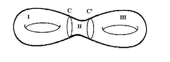
Figure 1: The double torus. The circles $C$ and $C^{\prime}$ represent the borders between regions I, II and III (see also fig.2).

Our purpose here is to build an example showing in explicit terms the validity of our general result in this special case. It will also be clear how to extend this example to the case of a pretzel with $g$ holes.

We decompose $\Lambda_{0}$ into three (flat) regions $B_{i}$ as suggested in fig.1; two of these are “tori with a cut”, while the central one is a cylinder. This is also illustrated in fig.2, where it is also shown how the three regions are glued together. (One could as well decompose it into two regions isomorphic to $B_{1}$ and $B_{3}$; we use the three-decomposition as this makes more clear the monodromy computation below.) With a slight abuse of notation, we will refer to the $B_{i}$ equipped with a coordinate system as “charts”, although each of these is actually the union of charts, and to their union as an atlas.

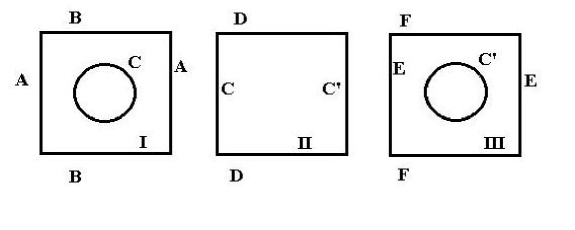
Figure 2: The decomposition of the double torus into three flat regions. The letters show which lines should be identified.

We take coordinates $(x_{i},y_{i})$ on each of the $B_{i}$. We can take the origin of the coordinate systems at the center of the rectangle representing each region; we take $x_{i},y_{i}$ to range from $-\pi$ to $\pi$ for $i=1,3$, and state for ease of discussion – but with no loss of generality – that for the central chart $x_{2}\in[-1,1]$, $y_{2}\in[-\pi,\pi]$.

The $B_{i}$ are immediately extended to charts (in the same sense, i.e. with the same abuse of notation, as above) and to an atlas on a tubular neighbourhood $U_{0}\subset{\mathcal{P}}\times{\mathcal{Q}}$ of $\Lambda_{0}$ of width $\varepsilon$; the coordinates on the chart $A_{i}$ built over $B_{i}$ will simply be $(x_{i},y_{i},z_{i};\lambda)$.

We define two vector fields on each of the $A_{i}$, given in local coordinates by

$$X_{i}\ :=\ {\partial\over\partial x_{i}}\ +\ \varphi_{i}(x_{i},y_{i},z_{i};\lambda){\partial\over\partial z_{i}}\ ;\ Y_{i}\ :=\ {\partial\over\partial y_{i}}\ +\ \psi_{i}(x_{i},y_{i},z_{i};\lambda){\partial\over\partial z_{i}}\ .$$

Note that in order for $\Lambda_{0}$ to be invariant under these, we must require that $\varphi_{i}$ and $\psi_{i}$ vanish on $\Lambda_{0}$, i.e. that $\varphi_{i}(x_{i},y_{i},0;0)=0$, $\psi_{i}(x_{i},y_{i},0;0)=0$.

If we linearize in the “vertical coordinates” $z_{i}$ and in $\lambda$, with $f_{i}(x_{i},y_{i}):=\left(\partial\varphi_{i}/\partial z_{i}\right)_{\Lambda_{0}}$, $g_{i}(x_{i},y_{i}):=\left(\partial\psi_{i}/\partial z_{i}\right)_{\Lambda_{0}}$, and similarly ${\widehat{f}}_{i}(x_{i},y_{i}):=\left(\partial\varphi_{i}/\partial\lambda\right)_{\Lambda_{0}}$, ${\widehat{g}}_{i}(x_{i},y_{i}):=\left(\partial\psi_{i}/\partial\lambda\right)_{\Lambda_{0}}$, we get

$$X_{i}\ :=\ {\partial\over\partial x_{i}}\ +\ \left(f_{i}z_{i}+{\widehat{f}}_{i}\lambda\right){\partial\over\partial z_{i}}\ ;\ Y_{i}\ :=\ {\partial\over\partial y_{i}}\ +\ \left(g_{i}z_{i}+{\widehat{g}}_{i}\lambda\right){\partial\over\partial z_{i}}\ .$$

A particularly simple but nontrivial choice (in which the vector field are chosen to be linear in $z$ and $\lambda$), corresponding to $f_{1}={\widehat{f}}_{1}=f_{3}={\widehat{f}}_{3}=0$, $f_{2}=q(x)$, ${\widehat{f}}_{2}=-q(x)b_{2}$, $g_{1}=g_{2}=g_{3}=1$, ${\widehat{g}}_{i}=-b_{i}$, is the following:

$$X_{i}:={\partial\over\partial x_{i}}+\delta_{i,2}\left[q(x)(z_{i}-b_{i}\lambda)\right]{\partial\over\partial z_{i}}\ ,\ Y_{i}:={\partial\over\partial y_{i}}+\left[z_{i}-b_{i}\lambda\right]{\partial\over\partial z_{i}}\ .$$

Here the $b_{i}$ are real constants, while $q(x)$ is a smooth function.

Let us now consider the transition regions $A_{i}\cap A_{j}$. For the sake of concreteness – and in order to introduce a notational simplification – let us just focus on $A_{1}\cap A_{2}$. We will write $x_{1}=\xi$, $y_{1}=\eta$, $z_{1}=\zeta$; $x_{2}=x$, $y_{2}=y$, $z_{2}=z$.

It is quite clear that we can just take $\zeta=z$, and that $\xi=\xi(x,y,z)$, $\eta=\eta(x,y,z)$ can be taken to be independent of $z$; so $z=\zeta$ (and of course the parameter $\lambda$) will just drop from our discussion of transition functions: these can be discussed in $B_{i}\cap B_{j}$.

It is convenient to use polar coordinates $(\rho,\vartheta)$ in $B_{1}$. For a point $(\xi,\eta)\simeq(x,y)\in B_{1}\cap B_{2}$, with our choice for the $x$ range and origin, $\rho=(\xi^{2}+\eta^{2})^{1/2}$ is just $\rho=r_{0}+(1+x)$, where $r_{0}$ is the radius of the excluded circle in $B_{1}$ (recall $0<r_{0}<1$); as this function will appear often in the following, we will denote it by $h(x)\ :=\ 1+r_{0}+x$.

As for the angle, we can just take $\vartheta=y$. Combining these with $\xi=\rho\cos(\vartheta)$ and $\eta=\rho\sin(\vartheta)$, we obtain at once the direct and inverse transition functions:

$$\begin{array}[]{ll}\xi\ =\ h(x)\,\cos(y)\ ;&\ \eta\ =\ h(x)\,\sin(y)\\ x\ =\ \sqrt{\xi^{2}+\eta^{2}}\,-\,(1+r_{0})\ ;&\ y\ =\ \arctan(\eta/\xi)\ .\end{array}$$

With the choice (5) for the vector fields, and the above, we get

$$\begin{array}[]{ll}X_{1}:=\left[\cos(y)\right]{\partial\over\partial x}-\left[{\sin(y)\over h(x)}\right]{\partial\over\partial y},&Y_{1}:=\left[\sin(y)\right]{\partial\over\partial x}+\left[{\cos(y)\over h(x)}\right]{\partial\over\partial y}+\left[z-b_{1}\lambda\right]{\partial\over\partial z}\ ;\\ X_{2}:={\partial\over\partial x}+\left[q(x)(z-b_{2}\lambda)\right]{\partial\over\partial z},&Y_{2}:={\partial\over\partial y}+\left[z-b_{2}\lambda\right]{\partial\over\partial z}\ .\end{array}$$

Let us now consider the commutation relations. It is easy to see that the condition (no sum over repeated indices from now on)

$$[X_{i},Y_{i}]\ =\ \sigma_{1}^{(i)}X_{i}+\sigma_{2}^{(i)}Y_{i}$$

which must be satisfied in each of the $A_{i}\backslash[\cup_{j\not=i}(A_{i}\cap A_{j})]$ for the vector fields to be in involution, actually imposes $\sigma_{1}^{(i)}=\sigma_{2}^{(i)}=0$, i.e. $[X_{i},Y_{i}]=0$ (so that again we can see one of $X$ and $Y$ as defining a dynamics, and the other as a symmetry of this dynamics). It is also easy to check that these are satisfied with our choice (5) for the vector fields.

Let us now discuss the commutation relations in the transition regions: in each of these four fields are present, and they should be in involution. Consider, for definiteness, $A_{1}\cap A_{2}$. By the Frobenius condition, we must require e.g. that there are functions $\sigma_{i}(x,y)$, $\mu_{i}(x,y)$, smooth in $A_{1}\cap A_{2}$, such that

$$[X_{1},X_{2}]\ =\ {\mathcal{S}}\ :=\ \sigma_{1}X_{1}+\sigma_{2}X_{2}+\mu_{1}Y_{1}+\mu_{2}Y_{2}\ ;$$

similar equations also hold for the other commutators.

One can check by explicit computations (see the appendix) that with our choice (5) for the vector fields, eq.(6) and those for the other relevant commutators admit a well defined solution under the condition that $\chi(x,y):=h(x)[q(x)-\sin(y)]$ does not vanish in $B_{1}\cap B_{2}$, i.e. for $r_{0}<x+1<r_{1}$, equivalently $-1<x<-1+\delta$.

As $h(x):=(1+x+r_{0})>0$ in $B_{1}\cap B_{2}$, we have to require that in this region $q(x)\not=\cos(y)$. We can e.g. require that for $-1<x<-1+\delta$ the function $q(x)$ satisfies $|q(x)|>1$. This leaves ample freedom of choice for that function.

Finally, we note that if $f_{i},g_{i}$ in (4’) are not zero, then there is no manifold near to $\Lambda_{0}$ (and homeomorphic to $\Lambda_{0}$) which is also invariant under these vector fields (this condition is relevant, in particular, if we are interested in bifurcations from invariant manifolds; see also the discussion in [18] for bifurcation from Poincaré-Lyapounov-Nekhoroshev invariant tori).

In order to illustrate our result, we have to consider the monodromy matrices associated to cycles providing a base for the homology of $\Lambda_{0}$. We consider the cycles in $\Lambda_{0}$ illustrated in figs.3 and 4.

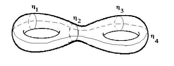
Figure 3: The four cycles, providing a basis for the homology of the double torus.

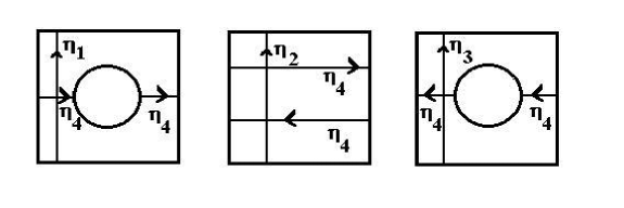
Figure 4: The four cycles, providing a basis for the homology of the double torus, here shown using the same representation as in fig.2.

Computation of the monodromy matrices for the cycles $\eta_{1},\eta_{2},\eta_{3}$ is immediate: each of these lies on a single region $B_{i}$, and moreover involve only $Y_{i}$. Along these paths, parametrized with $t\in[0,2\pi]$, we have (dropping the subscript $i$) $dx/dt=0$, $dy/dt=1$, $dz/dt=z-b\lambda$, $d\lambda/dt=0$; the solution for $z(t)$ (with $z(0)=z_{0}$) is given by

$$z(t)\ =\ e^{t-t_{0}}\,z_{0}\ +\ b\,\left(1-e^{t-t_{0}}\right)\,\lambda\ .$$

Therefore, writing $\kappa=\exp(2\pi)$, the monodromy matrix $M_{i}$ (coinciding with the monodromy map ${\mathcal{M}}_{i}$, as this is linear) and the associated $R_{i}$ are given by

$$M_{i}\ =\ \pmatrix{\kappa&(1-\kappa)b_{i}\cr 0&1\cr}\ ;\ R_{i}\ =\ \pmatrix{1-\kappa&(\kappa-1)b_{i}\cr 0&0\cr}\ .$$

The invariant local manifolds (under transport by $\nabla\equiv\nabla_{0}$ along $\eta_{i}$) are provided, as obvious from the explicit form of $Y_{i}$, by $z=b_{i}\lambda$. Needless to say, these local manifolds glue together into a global manifold if and only if $b_{1}=b_{2}=b_{3}=b$.

Let us now consider the path $\eta_{4}$ and the associated monodromy matrix $M_{4}$. The path $\eta_{4}$ is decomposed as $\tau_{4}\circ...\circ\tau_{1}$, see figure 4. With our choice of $X_{i}$, only the parts $\tau_{1}$ and $\tau_{3}$ will contribute to the monodromy map; that is, ${\dot{z}}=0$ for $\tau_{2}$ and $\tau_{4}$. As for $\tau_{1}$ and $\tau_{3}$, here ${\dot{x}}=1$, ${\dot{z}}=q(x)[z-b\lambda]$. We have therefore to solve ${\rm d}z/{\rm d}x=q(x)[z-b\lambda]$; writing in full generality $q(x)=Q^{\prime}(x)$, this has solution

$$z(x)\ =\ b\lambda\ +\ \exp\left[Q(x)-Q(x_{0})\right]\,(z_{0}-b\lambda)$$

for initial datum $z(x_{0})=z_{0}$. Note this, like the equation for $z(x)$ itself, is independent of $y$.

It is easy to see from the above expression and simple algebra (or directly from the $y$-independence) that the monodromy map $M_{4}:(z_{0},\lambda)\mapsto(z_{2},\lambda)$ is the identity. (It should be stressed that this is true not only of the linearized map, but of the full monodromy map, whenever $\varphi(x,y,z;\lambda)=\varphi(x,y+\pi,z;\lambda)$ or does not depend on $y$. See, in this respect, the third remark at the end of section 6.)

In conclusion, we have checked that – as actually obvious from the form of the vector fields – the smooth family of manifolds identified by $z=b\lambda$ is invariant under ${\mathcal{G}}$.

9 Example III

We will now provide a framework where the situation considered in example II is met in practice.

Hamiltonian systems with nontrivial topology of the relevant energy manifold have been studied by a number of authors, see e.g. [23], and [19] for a recent contribution focusing on isochronous hamiltonian systems; isochronous systems on Riemann surfaces extremely robust under perturbations have been considered by Calogero [8]. Here we discuss simpler systems; the quantum version of these is studied in [9].

We consider a system (not necessarily hamiltonian) describing a point particle in $R^{4}$, with cartesian coordinates $(x,y,z,w)$. We also introduce ”bi-polar” coordinates $(r_{1},\vartheta_{1},r_{2},\vartheta_{2})$ by

$$\begin{array}[]{ll}x=r_{1}\cos\vartheta_{1}\ ,&y=r_{1}\sin\vartheta_{1}\ ,\\ z=r_{2}\cos\vartheta_{2}\ ,&w=r_{2}\sin\vartheta_{2}\ .\end{array}$$

With $r_{j}=\sqrt{I_{j}}$ and $x=p_{1}$, $y=q_{1}$, $z=p_{2}$, $w=q_{2}$, we would be in a hamiltonian framework and $(I,\vartheta)$ be action-angle coordinates.

In these terms, the phase space is described as

$${\mathcal{P}}\ =\ {\bf T}^{2}\times{\bf R}_{+}^{2}\ .$$

Let us now introduce in ${\bf R}^{4}$ a solid cone ${\mathcal{C}}$ of angle $\Phi$, with vertex in the origin and surface $\partial{\mathcal{C}}$ described in the bi-polar coordinates by

$$\vartheta_{1}^{2}\,+\,\vartheta_{2}^{2}\ =\ \Phi^{2}\ .$$

This will be a solid surface on which the point particle bounces elastically. Thus, the accessible phase space ${\mathcal{P}}_{a}={\mathcal{P}}\backslash{\mathcal{C}}$ will be described in bi-polar coordinates as

$${\mathcal{P}}_{a}\ =\ {\bf T}^{2}_{\Phi}\times{\bf R}_{+}^{2}\ ,$$

where ${\bf T}^{2}_{\Phi}$ is the torus $(\vartheta_{1},\vartheta_{2})\in S^{1}\times S^{1}$ without the two-dimensional disk $D^{2}_{\Phi}$ of radius $\Phi$, see (7), ${\bf T}^{2}_{\Phi}={\bf T}^{2}\backslash D^{2}_{\Phi}$.

Note that each time the particle hits on the surface $\partial{\mathcal{C}}$, the component $p_{0}$ of its momentum in the direction orthogonal to the surface is reflected into $-p_{0}$, while other components of momentum – and a fortiori its position – are continuous. The motion takes then place normally until next hit on the surface, when again $p_{0}$ is reflected into $-p_{0}$ and so on. We can thus represent the motion as taking place on a double covering ${\mathcal{M}}$ of ${\mathcal{P}}_{a}$, the two sheets of this Riemann surface merging precisely on $\partial{\mathcal{C}}$. Needless to say, this construction is just a manifestation of the classical Schwarz reflection principle.

We would now like to present some remarks concerning this construction.

• (a) First of all, note that the dynamics is singular – and actually not uniquely defined – on $S^{1}_{0}:=\partial{\mathcal{C}}$; indeed, on these points the dynamics is defined by continuity and thus in particular it depends on the direction of approach (from one or the other of the two sheets of the double covering ${\mathcal{M}}$).

• (b) In view of our construction, it is entirely natural to consider a two-charts decomposition of $\Lambda_{0}$, each chart being isomorphic to ${\mathcal{P}}_{a}$ and corresponding to one sheet of the double covering ${\mathcal{M}}$; see fig.5. This also prompts for a different choice of the basis cycles for the homology of $\Lambda_{0}$, see fig.6.

• (c) Our construction implies the vector fields to be considered do naturally satisfy an antisymmetry condition with respect to $S^{1}_{0}$. This simplifies the computation of monodromy matrices, in particular if we adopt an appropriate choice for the basis cycles, each of them lying in a single chart of the double covering: indeed, it suffices then to compute the monodromy for cycles belonging to a given chart.

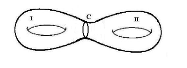
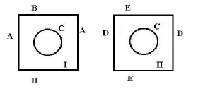
Figure 5: The decomposition of the double torus as two copies of ${\mathcal{P}}_{a}$, see text.

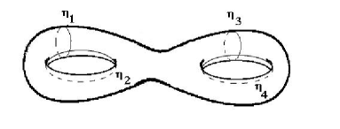
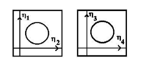
Figure 6: The four cycles providing a basis for the homology of the double torus, chosen in the natural way for the framework of example III (see text) and represented as in figg.3 and 4.

It suffice now to consider a simple ”unperturbed” system such as

$$\cases{{\dot{r}_{1}}=\alpha(r_{1},r_{2})&\cr{\dot{r}_{2}}=\beta(r_{1},r_{2})&\cr{\dot{\vartheta}_{1}}=\omega_{1}(r_{1},r_{2})&\cr{\dot{\vartheta}_{2}}=\omega_{2}(r_{1},r_{2})&\cr}$$

to get, with simple hypotheses on $\alpha,\beta,\omega_{1},\omega_{2}$ – e.g. that there are $\rho_{1},\rho_{2}$ such that $\alpha(\rho_{1},\rho_{2})=0=\beta(\rho_{1},\rho_{2})$, and $\omega_{1}(\rho_{1},\rho_{2})\not=0$, $\omega_{2}(\rho_{1},\rho_{2})\not=0$ – that the system admits a double torus $\Lambda_{0}$ in ${\mathcal{M}}$ as an invariant manifold. This corresponds to the situation discussed in example II.

If we then smoothly perturb the system, it is natural to ask if $\Lambda_{0}$ is somehow preserved (upon smooth deformation) in the perturbed system. Our theorem allows to answer this question.

Finally, it should be stressed that the system considered in this example could be hamiltonian, and more specifically a hamiltonian perturbation of a hamiltonian integrable system – or also, staying within the original framework of Nekhoroshev’s theorem [1], a partially integrable hamiltonian system.

In this case the unperturbed system would preserve all double tori being the double covering of (the part of) an invariant torus in ${\mathcal{P}}_{a}$, and we would be in the standard case of perturbation of an integrable or partially integrable system; however – as well known – the impact conditions would cause the system to be generically chaotic on the invariant double torus.

With our construction we are able to deal with the case of perturbation of integrable systems with impacts, at least for what concerns preservation upon deformation of the invariant double tori (the construction can also be generalized to more complex situations).

Note that in this case one should just compute monodromy on the standard invariant torus (see point (c) above); hence in this framework we just extended the validity of the Poincaré-Lyapounov-Nekhoroshev’s theorem [1, 17] to a class of systems with elastic impacts.

Appendix. Explicit formulas for example II

In this appendix we provide explicit solutions to equation (6) and similar ones for other relevant commutators in the transition region $A_{1}\cap A_{2}$ (similar ones hold for $A_{2}\cap A_{3}$). We recall that we have chosen the vector fields to be given by formula (5).

We define

$${\mathcal{S}}\ :=\ \sigma_{1}X_{1}+\sigma_{2}X_{2}+\mu_{1}Y_{1}+\mu_{2}Y_{2}$$

(it turns out we can choose e.g. $\mu_{2}=0$) and, for ease of writing,

$$\eta(x,y)\ :=\ q(x)-\sin(y)\ ;\ \chi(x,y):=h(x)\,\eta(x,y)\ .$$

We look first for solutions to $[X_{1},Y_{2}]\ =\ {\mathcal{S}}$. With our conventions, a solution to this is provided by

$$\sigma_{1}={\cos(y)\over\eta(x,y)}\ ,\ \sigma_{2}=-{1\over\eta(x,y)}\ ,\ \mu_{1}={q(x)\over\eta(x,y)}\ ,\ \mu_{2}=0\ .$$

The equation $[X_{1},X_{2}]={\mathcal{S}}$ is satisfied with

$$\begin{array}[]{rl}\sigma_{1}=&-\left[h(x)q^{\prime}(x)\cos^{2}(y)\,+\,\sin(y)\,-\,q(x)\sin^{2}(y)\right]\,/\,\chi(x,y)\ ,\\ \sigma_{2}=&\left[\cos(y)\,\left(h(x)q^{\prime}(x)\,+\,\sin(y)\right)\right]\,/\,\chi(x,y)\ ,\\ \mu_{1}=&-\left[\sin(y)\cos(y)\,\left(h(x)q^{\prime}(x)\,+\,q(x)\right)\right]\,/\,\chi(x,y)\ ,\\ \mu_{2}=&0\ .\end{array}$$

The equation $[Y_{1},X_{2}]={\mathcal{S}}$ is satisfied with

$$\begin{array}[]{rl}\sigma_{1}=&-\left[\cos(y)\,\left(\sin(y)\left(h(x)q^{\prime}(x)+q(x)\right)-1\right)\right]\,/\,\chi(x,y)\ ,\\ \sigma_{2}=&-\left[\cos^{2}(y)\,-\,h(x)q^{\prime}(x)\sin(y)\right]\,/\,\chi(x,y)\ ,\\ \mu_{1}=&\left[q(x)\cos^{2}(y)\,-\,h(x)q^{\prime}(x)\sin^{2}(y)\right]\,/\,\chi(x,y)\ ,\\ \mu_{2}=&0\ .\end{array}$$

Finally, the equation $[Y_{1},Y_{2}]={\mathcal{S}}$ is satisfied with

$$\sigma_{1}=-1\ ,\ \sigma_{2}=\mu_{1}=\mu_{2}=0\ .$$

Note that all of these are smooth in $B_{1}\cap{\mathcal{B}}_{2}$, and hence in ${\widehat{A}}_{1}\cap{\widehat{A}}_{2}$, provided $\chi(x,y):=h(x)[q(x)-\sin(y)]$ is nowhere zero in $B_{1}\cap B_{2}$.

References

- [1] N.N. Nekhoroshev, “The Poincaré-Lyapounov-Liouville-Arnol’d theorem”, Funct. Anal. Appl. 28 (1994), 128-129
- [2] W. Ambrose and I.M. Singer, “A theorem on holonomy”, Trans. A.M.S. 75 (1953), 428-443
- [3] A. Ambrosetti and G. Prodi, A primer of nonlinear analysis, Cambridge University Press, Cambridge, 1993.
- [4] V.I. Arnold, Mathematical methods of classical mechanics, Springer, Berlin, 1983, 1989.
- [5] V.I. Arnold, Geometrical methods in the theory of ordinary differential equations, Springer, Berlin, 1983, 1989.
- [6] D. Bambusi and G. Gaeta, “On persistence of invariant tori and a theorem by Nekhoroshev”, El. J. Math. Phys. 8 (2002), 1-13
- [7] D. Bambusi and D. Vella, “Quasi periodic breathers in hamiltonian lattices with symmetry”, Discr. Cont. Dyn. Syst. B (DCDS-B 2 (2002), 389-400
- [8] F. Calogero Classical many-body problems amenable to exact treatments, Springer, Berlin 2001
- [9] B.K. Cheng, “The two-dimensional harmonic oscillator interacting with a wedge”, J. Phys. A 23 (1990), 5807-5814
- [10] S.S. Chern, W.H. Chen and K.S. Lam, Lectures on Differential Geometry, World Scientific, Singapore 1999
- [11] G. Cicogna and G. Gaeta, Symmetry and perturbation theory in nonlinear dynamics, Springer, Berlin, 1999
- [12] M. Demazure, Bifurcation and catastrophes, Springer, Berlin, 2000
- [13] J.J. Duistermaat and J.A.C. Kolk, Lie Groups, Springer, Berlin, 2000
- [14] E. Fiorani, “Completely and partially integrable hamiltonian systems in the noncompact case”, Int. J. Geom. Meth. Mod. Phys. 1 (2004), 167-183
- [15] E. Fiorani, G. Giachetta and G. Sardanashvily, “The Liouville-Arnold-Nekhoroshev theorem for non-compact invariant manifolds”, J. Phys. A 36 (2003), L101-L107; “An extension of the Liouville-Arnold theorem for the non-compact case”, Nuovo Cimento B 118 (2003), 307-317
- [16] G. Gaeta, Nonlinear symmetries and nonlinear equations, Kluwer, Dordrecht, 1994
- [17] G. Gaeta, “The Poincaré-Lyapounov-Nekhoroshev theorem”, Ann. Phys. (N.Y.) 297 (2002), 157-173
- [18] G. Gaeta, “The Poincaré-Nekhoroshev map”, J. Nonlin. Math. Phys. 10 (2003), 51-64
- [19] L. Gavrilov, “Isochronicity of plane polynomial hamiltonian systems”, Nonlinearity 10 (1997), 433-448
- [20] G. Giachetta, L. Mangiarotti and G. Sardanashvily, “Bi-hamiltonian partially integrable systems”, J. Math. Phys. 44 (2003), 1984-1997
- [21] P. Glendinning, Stability, instability and chaos: an introduction to the theory of nonlinear differential equations, Cambridge University Press, Cambridge, 1994
- [22] J. Guckenheimer and P. Holmes, Nonlinear oscillations, dynamical systems, and bifurcation of vector fields, Springer, Berlin, 1983
- [23] V.V. Kozlov Symmetry, topology and resonances in Hamiltonian mechanics, Springer, Berlin 1996
- [24] M. Nakahara, Geometry, topology and physics, I.O.P., Bristol, 1990; 2nd ed. 2003
- [25] P.J. Olver, Applications of Lie groups to differential equations, Springer, Berlin, 1986
- [26] D. Ruelle, Elements of differentiable dynamics and bifurcation theory, Academic Press, London, 1989
- [27] D.J. Saunders, “A new approach to the nonlinear connection associated with second-order (and higher-order) differential equation fields”, J. Phys. A 30 No 5 (7 March 1997) 1739-1743
- [28] H. Stephani, Differential equations. Their solution using symmetries, Academic Press, London, 1989
- [29] S. Sternberg, Differential Geometry, Chelsea, N.Y., 1964; 2nd ed. 1983
- [30] F. Verhulst, Nonlinear differential equations and dynamical systems, Springer, Berlin, 1989, 1996