Dynamic Depletion of Vortex Stretching and Non-Blowup of the 3-D Incompressible Euler Equations

Abstract

We study the interplay between the local geometric properties and the non-blowup of the 3D incompressible Euler equations. We consider the interaction of two perturbed antiparallel vortex tubes using Kerr’s initial condition [14][Phys. Fluids 5 (1993), 1725]. We use a pseudo-spectral method with resolution up to $1536\times 1024\times 3072$ to resolve the nearly singular behavior of the Euler equations. Our numerical results demonstrate that the maximum vorticity does not grow faster than double exponential in time, up to $t=19$, beyond the singularity time $t=18.7$ predicted by Kerr’s computations [14, 17]. The velocity, the enstrophy and enstrophy production rate remain bounded throughout the computations. As the flow evolves, the vortex tubes are flattened severely and turned into thin vortex sheets, which roll up subsequently. The vortex lines near the region of the maximum vorticity are relatively straight. This local geometric regularity of vortex lines seems to be responsible for the dynamic depletion of vortex stretching.

1 Introduction

One of the most challenging questions in fluid dynamics is whether the incompressible 3D Euler equations can develop a finite time singularity from smooth and bounded initial data. From a theoretical point of view, the main difficulty is due to the presence of the vortex stretching term in the vorticity equation, which is formally quadratic in vorticity. If such quadratic nonlinearity persists in time long enough, we would expect a finite time singularity of the form $O(T-t)^{-1}$ in vorticity. Such blow-up rate is consistent with the well-known result of Beale-Kato-Majda [2] (see also [11]). There have been many computational efforts in searching for finite time singularities of the 3D Euler and Navier-Stokes equations, see e.g. [6, 22, 18, 13, 23, 14, 5, 3, 21, 12, 17, 24]. One example that has been studied extensively is the interaction of two perturbed antiparallel vortex tubes. This example is interesting because of the vortex reconnection which has been observed for the corresponding Navier-Stokes equations. It is natural to ask whether the 3D Euler equations would develop a finite time singularity in the limit of vanishing viscosity.

In [14], Kerr presented numerical evidence which suggests a finite time singularity of the 3D Euler equations for two perturbed antiparallel vortex tubes. In Kerr’s computations, he used a pseudo-spectral discretization in the $x$ and $y$ directions, and a Chebyshev discretization in the $z$ direction with resolution of order $512\times 256\times 192$. His computations showed that the growth of the peak vorticity, the peak axial strain, and the enstrophy production obey $(T-t)^{-1}$ with $T=18.9$. Self-similar development and equal rates of collapse in all three directions were shown (see the abstract of [14]). While velocity blowup was not documented in [14], Kerr showed in his subsequent papers [15, 16, 17] that velocity field blows up like $O(T-t)^{-1/2}$ with $T$ being revised to $T=18.7$. Kerr’s computations have generated a lot of interests and his proposed initial conditions have been considered as “the most attractive candidates for potential singular behavior” of the 3D Euler equations (see page 187 of [19]).

Vortex reconnection of two perturbed antiparallel vortex tubes has been studied extensively in the literature. Substantial core deformation has been observed [22, 1, 4, 18, 20, 23]. Most studies indicated only exponential growth in the maximum vorticity. However, the work of Kerr and Hussain in [18] suggested a finite time blow-up in the infinite Reynolds number limit, which motivated Kerr’s Euler computations mentioned above.

There has been some interesting development in the theoretical understanding of the 3D incompressible Euler equations. It has been shown that the local geometric regularity of vortex lines can play an important role in depleting nonlinear vortex stretching [7, 8, 9, 10]. In particular, the recent results obtained by Deng, Hou, and Yu [9, 10] show that geometric regularity of vortex lines, even in an extremely localized region containing the maximum vorticity, can lead to depletion of nonlinear vortex stretching, thus avoiding finite time singularity formation of the 3D Euler equations. To obtain these results, Deng-Hou-Yu [9, 10] explored the connection between the stretching of local vortex lines and the growth of vorticity. In particular, they showed that if the vortex lines near the region of maximum vorticity satisfy some local geometric regularity conditions and the maximum velocity field is integrable in time, then no finite time blow-up is possible. See Section 4.2 for the detailed description of these results. Kerr’s computations fall in the critical case of the non-blowup theory in [9, 10]. To get a definite answer in this critical case, we need to check whether certain scaling constants, which describe the local geometric properties of the vortex lines, satisfy an algebraic inequality. However, such scaling constants are not available in [14]. This is our original motivation to repeat Kerr’s computations.

It is worth mentioning that the predicted singularity time in Kerr’s computations is $T=18.7$, while his computations from $t=17$ to $t=18$, as mentioned in [14], seem to be under-resolved and were “not part of the primary evidence for a singularity”. Clearly, the computations for $t\leq 17$, which Kerr used as the primary evidence for a singularity, is still far from the predicted singularity time, $T=18.7$. In order to justify the predicted asymptotic behavior of vorticity and velocity blowup, one needs to perform well-resolved computations much closer to the predicted singularity time. Such well-resolved computations can also provide more accurate geometric properties of vortex lines, which can be used to check whether the non-blowup conditions in [9, 10] are satisfied.

In this paper, we perform well-resolved computations of the 3D incompressible Euler equations using the same initial condition as the one used by Kerr in [14]. A pseudo-spectral method with a very high order Fourier smoothing is used to discretise the 3D incompressible Euler equations in all three directions. The time integration is performed using the classical fourth order Runge-Kutta method with adaptive time stepping to satisfy the CFL stability condition. We perform a careful numerical study to show that the pseudo-spectral method we use provides more accurate approximations to the 3D Euler equations than the pseudo-spectral method that uses the standard 2/3 dealiasing rule. We use up to $1536\times 1024\times 3072$ space resolution in order to resolve the nearly singular behavior of the 3D Euler equations.

Our numerical results demonstrate that the maximum vorticity does not grow faster than double exponential in time, up to $t=19$, beyond the singularity time $t=18.7$ predicted by Kerr’s computations [14, 17]. There are three distinguished stages of vorticity growth in time. In the early stage for $0\leq t\leq 12$, the maximum vorticity grows only exponentially in time. During the intermediate stage for $12\leq t\leq 17$, the two vortex tubes experience tremendous core deformation and become severely flattened. Each vortex tube effectively turns into a vortex sheet with rapidly decreasing thickness. During this stage, the maximum vorticity grows slightly slower than double exponential in time. It is also interesting to examine the degree of nonlinearity in the vortex stretching term during this stage. An $O(T-t)^{-1}$ blowup rate in the maximum vorticity would imply that the nonlinearity in the vortex stretching term is quadratic. However, our numerical results show that the vortex stretching term, when projected to the unit vorticity vector, is bounded by $\|\vec{\omega}\|_{\infty}\log(\|\vec{\omega}\|_{\infty})$, where $\vec{\omega}$ is vorticity. It is easy to see that such upper bound on the vortex stretching term implies that the maximum vorticity is bounded by double exponential in time. During the final stage for $17\leq t\leq 19$, we observe that the growth of the maximum vorticity slows down considerably and deviates from double exponential growth, indicating that there is stronger cancellation taking place in the vortex stretching term.

We also find that the vortex lines near the region of the maximum vorticity are relatively straight and the vorticity vectors seem to be quite regular. This was also observed in [14]. On the other hand, the inner region containing the maximum vorticity does not seem to shrink to zero at a rate of $(T-t)^{1/2}$, as predicted by Kerr’s computations. Moreover, we find that the velocity field, the enstrophy, and enstrophy production rate remain bounded throughout the computations. The fact that the velocity field remains bounded is significant. With velocity field being bounded, the result of Deng-Hou-Yu [9] can be applied, which implies the non-blowup of the Euler equations up to $T=19$. The geometric regularity of the vortex lines near the inner region seems to play an important role in the dynamic depletion of vortex stretching [9, 10].

We would like to stress the importance of sufficient resolution in determining the nature of the nearly singular behavior of the 3D Euler equations. As demonstrated by our numerical computations, the 3D Euler equations have different growth rates in the maximum vorticity in different stages. A resolution without the proper level of refinement would not be able to capture the transition from one growth phase to another. In [14], the inverse of the maximum vorticity was shown to approach to zero almost linearly in time up to $t=17$. If this trend were to continue to hold, it would lead to the blowup of the maximum vorticity in the form of $O(T-t)^{-1}$. However, with increasing resolutions, we find that the curve corresponding to the inverse of maximum vorticity starts to turn away from zero starting at $t=17$. We also observe that the velocity field becomes saturated around this time. Incidentally, this is precisely the time when Kerr’s computations began to lose resolution. At $t=17$, the thin vortex sheets have already started to roll up. After $t=17.5$, the vorticity in the rolled up region has developed large gradients in all three directions, with $z$ being the most singular direction and $y$ being the least singular direction. To resolve the large gradients in all three directions, we allocate $3072$ grid points along the $z$ direction, $1536$ along the $x$ direction, and $1024$ along the $y$ direction. This level of resolution ensures that we have about 8 grid points across the most singular region in each direction toward the end of the computations.

Kerr interpreted the roll-up of the vortex sheet as “two vortex sheets meeting at an angle” and argued that the formation of this angle may be responsible for the finite time blowup of the Euler equations. Our computations indicate that the rollup region of the vortex sheet is still relatively smooth even during the final stage of the computations. Moreover, according to the results in [9, 10], it is the curvature of the vortex lines and the divergence of the unit vorticity vector that contribute to the blow-up, not the curvature of the vortex sheet itself. Further, we observe that the vortex lines near the region of the maximum vorticity are relatively smooth. This geometric regularity leads to strong dynamic depletion of the nonlinear vortex stretching.

There is reason to believe that if the current scenario persists, there is no blowup of the 3D Euler equations for these data beyond $T=19$. In fact, during the final stage of the computations for $17.5\leq t\leq 19$, the vortex lines near the region of the maximum vorticity remain smooth. Further, as the vortex sheet rolls up, we observe that the location of the maximum vorticity moves away from the dividing plane separating the two vortex tubes toward the rolled up portion of the vortex sheet, leading to a slower growth rate of maximum vorticity.

The rest of this paper is organized as follows. We describe the set-up of the initial condition in Section 2 and describe our numerical method in Section 3. In Section 4, we describe our numerical results in detail and perform comparisons with the previous results obtained in [14, 17]. Some concluding remarks are made in Section 5.

2 The Initial Condition

The 3D incompressible Euler equations in the vorticity stream function formulation are given as follows:

$$\vec{\omega}_{t}+(\vec{u}\cdot\nabla)\vec{\omega} = \nabla\vec{u}\cdot\vec{\omega},$$ (1)

$$-\bigtriangleup\vec{\psi} = \vec{\omega},\quad\vec{u}=\nabla\times\vec{\psi},$$ (2)

with initial condition $\vec{\omega}\mid_{t=0}=\vec{\omega}_{0}$, where $\vec{u}$ is velocity, $\vec{\omega}$ is vorticity, and $\vec{\psi}$ is stream function. Vorticity is related to velocity by $\vec{\omega}=\nabla\times\vec{u}$. The incompressibility implies that

$$\nabla\cdot\vec{u}=\nabla\cdot\vec{\omega}=\nabla\cdot\vec{\psi}=0.$$

We consider periodic boundary conditions with period $2\pi$ in all three directions.

We study the interaction of two perturbed antiparallel vortex tubes using the same initial condition as that of Kerr (see Section III of [14]). There are a few misprints in the analytic expression of the initial condition given in [14]. In our computations, we use the corrected version of Kerr’s initial condition by comparing with Kerr’s Fortran subroutine which was kindly provided to us by him. A list of corrections to these misprints is given in the Appendix.

The initial condition is given by a pair of perturbed anti-parallel vortex tubes, which is expressed in terms of vorticity. The vorticity that describes the vortex tube above the $x$-$y$ plane is of the form:

$$\vec{\omega}=\omega(r)(\omega_{x},\;\omega_{y},\;\omega_{z}).$$ (3)

The first step in setting up the initial condition is to define the profile $\omega(r)$. If $r\geq 1$, we set $\omega(r)=0$. For $r<1$, we define

$$\omega(r)=\exp[f(r)],$$ (4)

with $f(r)$ given by

$$f(r)=\frac{-r^{2}}{1-r^{2}}+r^{4}\left(1+r^{2}+r^{4}\right).$$ (5)

The radius $r$ is centered around an initial vortex core trajectory $(X,Y,Z)$, and is defined by

$$r=\left|\left(x,y,z\right)-\left(X,Y,Z\right)\right|/R,\hskip 20.00003pt\mathrm{for}\;\;r\leqslant 1.$$ (6)

The initial vortex core trajectory $(X,Y,Z)$ is characterized by

$$\left(X,Y,Z\right)=(x(s),y,z(s)),$$ (7)

where $s$ is a function of $y$ and

$$x(s)=x_{0}+\delta_{x}\cos(\pi s/L_{x}),$$ (8)

$$z(s)=z_{0}+\delta_{z}\cos(\pi s/L_{z}).$$ (9)

To complete the definition of $\omega(r)$, we need to define $s$ as a function of $y$, which is given below:

$$s(y)=y_{2}+L_{y}\delta_{y1}\sin(\pi y_{2}/L_{y}),$$ (10)

and

$$y_{2}=y+L_{y}\delta_{y2}\sin\left(\pi y/L_{y}\right).$$ (11)

The second step is to define the vorticity vector $(\omega_{x},\omega_{y},\omega_{z})$, which is given as follows:

$$\omega_{x} = -\frac{\pi\delta_{x}}{L_{x}}\left[1+\pi\delta_{y_{2}}\cos\left(\frac{\pi y}{L_{y}}\right)\right]\times\left[1+\pi\delta_{y1}\cos\left(\frac{\pi y_{2}}{L_{y}}\right)\right]\sin\left(\frac{\pi s(y)}{L_{x}}\right),$$ (12)

$$\omega_{y} = 1,$$ (13)

$$\omega_{z} = -\frac{\pi\delta_{z}}{L_{z}}\left[1+\pi\delta_{y_{2}}\cos\left(\frac{\pi y}{L_{y}}\right)\right]\times\left[1+\pi\delta_{y1}\cos\left(\frac{\pi y_{2}}{L_{y}}\right)\right]\sin\left(\frac{\pi s(y)}{L_{z}}\right).$$ (14)

We choose exactly the same parameters as in [14]. Specifically, we set $\delta_{y1}=0.5$, $\delta_{y2}=0.4$, $\delta_{x}=-1.6$, $\delta_{z}=0$, $z_{0}=1.57$ and $R=0.75$. The constant $x_{0}$ fixes the center of perturbation for the vortex tube along the $x$ direction. In our computations, we set $x_{0}=0$. Moreover, we choose $L_{x}=L_{y}=4\pi$, and $L_{z}=2\pi$.

The third step is to rescale the initial profile defined above. According to [14] (see the last paragraph on page 1728 of [14]), we need to rescale the above initial vorticity profile by a constant factor so that the maximum vorticity in the $y$ direction is increased to 8. With the choice of the above parameters, the maximum vorticity in the $y$ direction before rescaling is equal to 0.999766. Thus, the constant rescaling factor is equal to 8.001873.

The final step in defining the initial condition is to filter the initial vorticity profile. After rescaling the initial vorticity, we apply exactly the same Fourier filter as the one used in [14], i.e. $\exp\left[-0.05\left(k_{x}^{4}+k_{y}^{4}+k_{z}^{4}\right)\right]$, to the initial vorticity to smooth the rough edges.

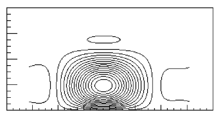
Figure 1: The axial vorticity ($\omega_{y}$) contours of the initial value on the symmetry plane.

We should point out that due to the difference between ours and Kerr’s discretization strategies in solving the 3D Euler equations, the discrete initial condition generated by Kerr’s discretization and the one generated by our pseudo-spectral discretization are not exactly the same. In [14], Kerr used the Chebyshev polynomials to approximate the solution along the $z$ direction. In order to prepare the initial data that can be used for the Chebyshev polynomials, he performed some interpolation and used extra filtering. This interpolation and extra filtering seem to introduce some asymmetry to Kerr’s discrete initial data. According to [14] (see the top paragraph of page 1729), “An effect of the initial filter upon the vorticity contours at $t=0$ is a long tail in Fig. 2(a)”. Since we perform pseudo-spectral approximations in all three directions, there is no need to perform interpolation or use extra filtering as was done in [14]. To demonstrate this slight difference between Kerr’s initial data and ours, we plot the initial vorticity contours along the symmetry plane in Figure 1. As we can see, the initial vorticity contours in Figure 1 are essentially symmetric. This is in contrast to the apparent asymmetry in Kerr’s initial vorticity contours (see Fig. 2(a) of [14]). The 3D plot of the initial vortex tubes is given in Figure 3. Again, we can see that the initial vortex tube is essentially symmetric. As time increases, the two antiparallel perturbed vortex tubes approach each other. By time $t=6$, we already observe a significant flattening near the center of the tubes, see Figure 2 and Figure 3.

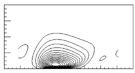
Figure 2: The axial vorticity ($\omega_{y}$) contours when $t=6$ on the symmetry plane.

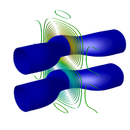
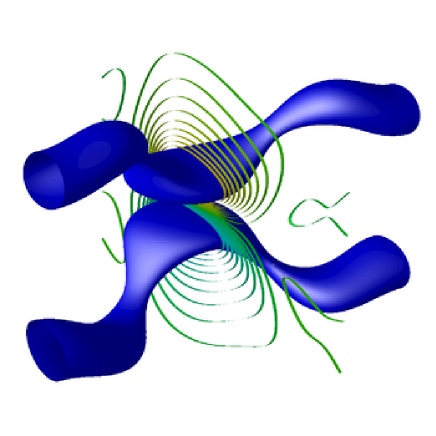
Figure 3: The 3D view of the vortex tube for $t=0$ and $t=6$. The tube is the isosurface at $60\%$ of the maximum vorticity. The ribbons on the symmetry plane are the contours at other different values.

3 The Numerical Method

We use the pseudo-spectral method with a very high order Fourier smoothing to discretize the 3D Euler equations. The Fourier smoothing that we use along the $x_{j}$ direction is of the form: $\rho(2k_{j}/N_{j})\equiv\exp(-\alpha(2k_{j}/N_{j})^{m})$ with $\alpha=36$ and $m=36$, where $k_{j}$ is the wave number ($|k_{j}|\leqslant N_{j}/2$) along the $x_{j}$ direction and $N_{j}$ is the total number of grid points along the $x_{j}$ direction. Specifically, if $\widehat{v}_{k}$ is the discrete Fourier transform of $v$, then we approximate $v_{x_{j}}$ by taking the discrete inverse Fourier transform of $ik_{j}\rho(2k_{j}/N_{j})\widehat{v}_{k}$, where $k=(k_{1},k_{2},k_{3})$. The time integration is performed using the classical fourth order Runge-Kutta method. Adaptive time stepping is used to satisfy the CFL stability condition with CFL number equal to $\pi/4$. We use up to $1536\times 1024\times 3072$ space resolution in order to resolve the nearly singular behavior of the 3D Euler equations.

There is a good reason why we choose to use the pseudo-spectral method with the above high order Fourier smoothing instead of using the classical 2/3 dealiasing rule. The Fourier smoothing we use is designed to keep the majority of the Fourier modes unchanged and remove the very high modes to avoid the aliasing errors, see Fig. 4 for the profile of $\rho(x)$. We choose $\alpha$ to be $36$ to guarantee that $\rho(k)$ reaches the level of the round-off errors ($O(10^{-16})$) at the highest modes. We choose the order of smoothing, $m$, to be 36 in order to optimize the accuracy of the spectral approximation, while still keeping the aliasing errors under control. As we can see from Figure 4, the effective modes in our computation are about $12\sim 15\%$ more than those using the standard $2/3$ dealiasing rule. To demonstrate that the pseudo-spectral method with the above high order Fourier smoothing is indeed more accurate than the pseudo-spectral method with the $2/3$ dealiasing rule, we perform resolution study of the two approaches. In Figure 5, we compare the Fourier spectra of the enstrophy obtained by using the pseudo-spectral method with the $2/3$ dealiasing rule with those obtained by the pseudo-spectral method with the high order smoothing. For a fixed resolution $768\times 512\times 1536$, we can see that the Fourier spectra obtained by the pseudo-spectral method with the high order smoothing are more accurate than those obtained by the spectral method using the $2/3$ dealiasing rule. This can be seen by comparing the results with the corresponding computations using a higher resolution $1024\times 768\times 2048$. Moreover, the pseudo-spectral method using the high order Fourier smoothing does not give the spurious oscillations in the Fourier spectra which are present in the computations using the $2/3$ dealiasing rule near the $2/3$ cut-off point.

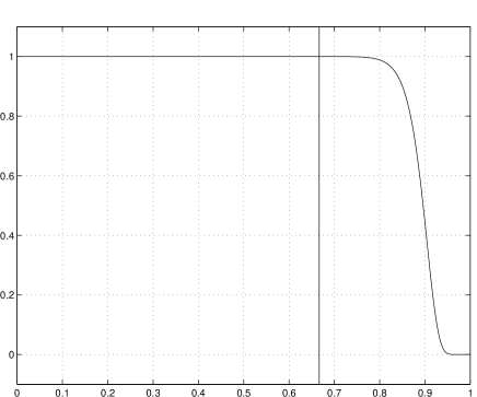
Figure 4: The profile of the Fourier smoothing: $\exp(-36(x)^{36})$. The vertical line corresponds to the cut-off mode using the $2/3$ dealiasing rule. We can see that using this Fourier smoothing we keep about $12\sim 15\%$ more modes than those using the 2/3 dealiasing rule.

We have used a sequence of resolutions in our computations in order to perform a resolution study. The resolutions presented in the paper are $768\times 512\times 1536$, $1024\times 768\times 2048$, and $1536\times 1024\times 3072$ respectively. Except for the computation on the largest resolution $1536\times 1024\times 3072$, all computations are carried out from $t=0$ to $t=19$. The computation on the final resolution $1536\times 1024\times 3072$ is started from $t=10$ with the initial condition given by the computation with the resolution $1024\times 768\times 2048$. From our resolution study for the velocity and vorticity in both physical and spectral spaces, we find that the solution at $t=10$ is fully resolved even on the resolution $768\times 512\times 1536$. Thus it is justified to start the computation with the largest resolution at $t=10$ using the computation obtained by the resolution $1024\times 768\times 2048$ as the initial condition.

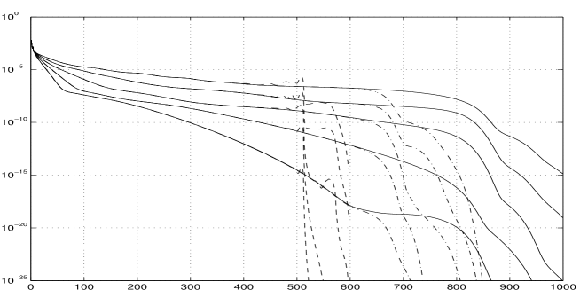
Figure 5: The comparison of the enstrophy spectra obtained using the high order Fourier smoothing method with those using the 2/3 dealiasing rule. The dashed lines and dashed-dotted lines are the enstrophy spectra with the resolution $768\times 512\times 1536$ using the 2/3 dealiasing rule and the Fourier smoothing, respectively. The solid lines are the enstrophy spectra with resolution $1024\times 768\times 2048$. The times for the spectra lines are at $t=15,16,17,18,19$ respectively.

We also exploit the symmetry properties of the solution in our computations, and perform our computations on only a quarter of the whole domain. We use the well-known parallel FFT package, called FFTW 3.1 to perform the sine and cosine transformations. The whole program is coded in C and we use MPI as the parallel interface. Since the solution appears to be most singular in the $z$ direction, we allocate twice as many grid points along the $z$ direction than along the $x$ direction. The solution is least singular in the $y$ direction. We allocate the smallest resolution in the $y$ direction to reduce the computation cost. In our computations, two typical ratios in the resolution along the $x$, $y$ and $z$ directions are $3:2:6$ and $4:3:8$.

In the early stage of the computations for $0\leq t\leq 8$, the solution is still very regular. The solution in this stage can be fully resolved using the resolution $768\times 512\times 1536$. In the intermediate stage for $8\leq t\leq 16$, the solution has a fast growth in the maximum vorticity. After $t=16$, the two vortex tubes become severely flattened, and evolve into two thin vortex sheets, which roll up subsequently. The maximum vorticity also experiences a transition from the double exponential growth to a slower growth rate due to the dynamic depletion of vortex stretching. In order to resolve the later stage of the solution, higher resolutions become necessary.

Our computations were carried out on the PC cluster LSSC-II in the Institute of Computational Mathematics and Scientific/Engineering Computing of Chinese Academy of Sciences and the Shenteng 6800 cluster in the Super Computing Center of Chinese Academy of Sciences. The maximal memory consumption in our computations is about 120 GBytes.

4 Numerical Results

4.1 Review of Kerr’s results

In [14], Kerr presented numerical evidence which suggested a finite time singularity of the 3D Euler equations for two perturbed antiparallel vortex tubes. He used a pseudo-spectral discretization in the $x$ and $y$ directions, and a Chebyshev method in the $z$ direction with resolution of order $512\times 256\times 192$. His computations showed that the growth of the peak vorticity, the peak axial strain, and the enstrophy production obey $(T-t)^{-1}$ with $T=18.9$. As $t$ approaches the alleged blow-up time $T$, the region bounded by the contour of $0.6\|\vec{\omega}\|_{\infty}$, also known as the inner region, looks like two vortex sheets with thickness $\sim(T-t)$ meeting at an angle [14]. This region has the length scale $(T-t)^{1/2}$ in the vorticity direction. The maximum vorticity resides in the small tube-like region, with scaling $(T-t)^{1/2}\times(T-t)\times(T-t)$, which is the intersection of the two sheets. Inside the inner region, the vortex lines are “relatively straight” [14]. Kerr stated in his paper [14] (see page 1727) that his numerical results shown after $t=17$ and up to $t=18$ were “not part of the primary evidence for a singularity” due to the lack of sufficient numerical resolution and the presence of noise in the numerical solutions.

In his recent paper [17] (see also [15, 16]), Kerr applied a high wave number filter to the data obtained in his original computations to “remove the noise that masked the structures in earlier graphics” presented in [14]. With this filtered solution, he presented some scaling analysis of the numerical solutions up to $t=17.5$. Two new properties were presented in this recent paper [17]. First, the velocity field was shown to blow up like $O(T-t)^{-1/2}$ with $T$ being revised to $T=18.7$. The maximum velocity is located on the boundary of the inner region with distance $(T-t)^{1/2}$ away from the position where the maximum vorticity is achieved. Secondly, he showed that the blowup is characterized by two anisotropic length scales, $\rho\approx(T-t)$ and $R\approx(T-t)^{1/2}$. Further, Kerr argued that the curvature, $\kappa$, of the vortex lines and $\nabla\cdot\vec{\xi}$ (here $\vec{\xi}=\vec{\omega}/|\vec{\omega}|$) in the inner region are likely bounded by $(T-t)^{-1/2}$ [17].

4.2 Recent theoretical results on the 3D Euler equations

There has been some interesting development in the theoretical understanding of the 3D incompressible Euler equations. It has been shown by several authors that the local geometric regularity of vortex lines can play an important role in depleting nonlinear vortex stretching. In particular, Constantin, Fefferman and Majda [8] proved that if (i) there is up to time $T$ an $O(1)$ region $\Omega$ in which the vorticity vector is smoothly directed, i.e., the maximum norm of $\nabla\xi$ in this $O(1)$ region is $L^{2}$ integrable in time, (ii) the maximum norm of velocity is uniformly bounded in time, plus a technical condition on the distribution of the vorticity within this region, then no blow-up can occur in this region up to time $T$. While this result is very interesting, it does not apply to Kerr’s computations since the two assumptions are violated by Kerr’s computations.

Motivated by the result of [8], Deng, Hou, and Yu [9] obtained sharper non-blowup conditions which use only very localized information of the vortex lines. Assume that at each time $t$ there exists some vortex line segment $L_{t}$ on which the local maximum vorticity is comparable to the global maximum vorticity. Further, we denote $L(t)$ as the arclength of $L_{t}$. Roughly speaking, if (i) the velocity field along $L_{t}$ is bounded by $C_{U}(T-t)^{-\alpha}$ for some $\alpha<1$, (ii) $C_{L}(T-t)^{\beta}\leq L(t)\leq C_{0}/\max_{L_{t}}(|\kappa|,\;|\nabla\cdot\vec{\xi}|)$, for some $\beta<1-\alpha$, then the solution of the 3D Euler equations remains regular up to $T$. In Kerr’s computations, the first condition is satisfied with $\alpha=1/2$. Moreover, based on the bound on $\kappa$ and $\nabla\cdot\vec{\xi}$ in the inner region [17], we can choose a vortex line segment of length $(T-t)^{1/2}$ in the inner region so that the upper bound in the second condition is satisfied. However, the lower bound is violated since $\beta<1/2=1-\alpha$. In a subsequent paper [10], the non-blowup conditions have been improved to include the critical case, $\beta=1-\alpha$ by requiring the scaling constants, $C_{U},\;C_{0},$ and $C_{L}$ in conditions (i)-(ii), to satisfy an algebraic inequality. This algebraic inequality can be checked numerically if we obtain a good estimate of these scaling constants. For example, if $C_{0}=0.1$, which seems reasonable since the vortex lines are relatively straight in the inner region, the result of [10] implies no blowup up to $T$ if $2C_{U}<0.43C_{L}$. However, such scaling constants are not available in [14]. One of our original motivations was to repeat Kerr’s computations with higher resolution to obtain a good estimate of these scaling constants.

4.3 Maximum vorticity growth

We first present the result on the growth of the maximum vorticity in time, see Figure 6. The maximum vorticity increases rapidly from the initial value of $0.669$ to $23.46$ at the final time $t=19$, a factor of 35 increase from its initial value. Kerr’s computations predicted a finite time singularity at $T=18.7$. Our computations show no sign of finite time blowup of the 3D Euler equations up to $T=19$, beyond the singularity time predicted by Kerr. In Figure 6, we plot the maximum vorticity in time using three different resolutions, i.e. $768\times 512\times 1536$, $1024\times 768\times 2048$, and $1536\times 1024\times 3072$ respectively. As we can see, the agreement between the two successive resolutions is very good with only mild disagreement toward the end of the computations. This indicates that a very high space resolution is indeed needed to capture the rapid growth of maximum vorticity at the later stage of the computations.

We observe that the growth of the maximum vorticity has three distinguished phases. The first stage is for $0\leq t\leq 12$. In this early stage, the maximum vorticity grows only exponentially in time. This is consistent with Kerr’s results. The second stage is for $12\leq t\leq 17$. During this intermediate stage, the two vortex tubes experience tremendous core deformation and become severely flattened. Each vortex tube effectively turns into a vortex sheet with rapidly decreasing thickness. We observe that the growth of maximum vorticity is slightly slower than double exponential in time during the second stage, see Figure 7. This growth behavior can be also confirmed by examining the degree of nonlinearity in the vortex stretching term. If the maximum vorticity indeed blew up like $O(T-t)^{-1}$, as alleged in [14], the vortex stretching term at the position of the maximum vorticity should have been quadratic as a function of maximum vorticity. However, as Figure 8 shows, the vortex stretching term, when projected to the unit vorticity vector, grows much slower than the quadratic nonlinearity. In fact, it is even slower than $C\|\vec{\omega}\|_{\infty}\log(\|\vec{\omega}\|_{\infty})$, i.e.

$$\|\vec{\xi}\cdot\nabla\vec{u}\cdot\vec{\omega}\|_{\infty}\leq C\|\vec{\omega}\|_{\infty}\log(\|\vec{\omega}\|_{\infty}),\quad\quad 15\leq t\leq 19.$$ (15)

Using the equation that governs the magnitude of vorticity [7],

$$\frac{\partial}{\partial t}|\vec{\omega}|+(\vec{u}\cdot\nabla)|\vec{\omega}|=\vec{\xi}\cdot\nabla\vec{u}\cdot\vec{\omega},$$ (16)

one can easily show that inequality (15) implies that the maximum vorticity is bounded by double exponential in time.

During the final stage for $17\leq t\leq 19$, we observe that the growth of the maximum vorticity slows down and deviates from double exponential growth, see Figure 7. This indicates that there is stronger cancellation taking place in the vortex stretching term.

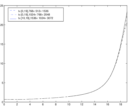
Figure 6: The maximum vorticity $\|\omega\|_{\infty}$ in time using different resolutions.

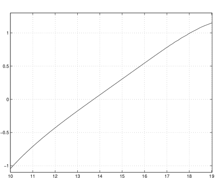
Figure 7: The plot of $\log\log\|\omega\|_{\infty}$ vs time, resolution $1536\times 1024\times 3072$.

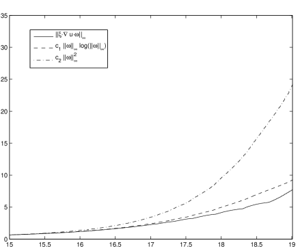
Figure 8: Study of the vortex stretching term in time, resolution $1536\times 1024\times 3072$. We take $c_{1}=1/8.128$, $c_{2}=1/23.24$ to match the same starting value for all three plots.

We remark that for vorticity that grows as rapidly as double exponential in time, one may be tempted to fit the maximum vorticity growth by $(T-t)^{-1}$ for some $T$. Indeed, if we choose $T=18.7$ as suggested by Kerr in [17], we find a reasonably good fit for the maximum vorticity as a function of $c/(T-t)$ for the period $15\leq t\leq 17$. We plot the scaling constant $c$ in Figure 9. As we can see, $c$ is close to a constant for $15\leq t\leq 17$. To conclude that the 3D Euler equations indeed develop a finite time singularity, one must demonstrate that such scaling persists as $t$ approaches to $T$. As we can see from Figure 9, the scaling constant $c$ decreases rapidly to zero as $t$ approaches to the alleged singularity time $T$. Therefore, the fitting of $\|\vec{\omega}\|_{\infty}\approx O(T-t)^{-1}$ is not correct asymptotically.

A similar test can be performed for the inverse of the maximum vorticity. In Figure 10, we plot the inverse of the maximum vorticity using different resolutions. As we can see from this picture, the inverse of the maximum vorticity approaches to zero almost linearly in time for $8\leq t\leq 17$. This was one of the strong evidences presented in [14] that suggests a finite time blowup of the 3D Euler equations. If this trend were to continue to hold up to $T$, it would have led to the blowup of the maximum vorticity in the form of $O(T-t)^{-1}$. However, as we increase our resolutions, we find that the curve corresponding to the inverse of the maximum vorticity starts to turn away from zero around $t=17$. This is precisely the time when Kerr’s computations began to lose resolution. By $t=17.5$, the gradients of the solution become very large in all three directions. In order to resolve the nearly singular solution structure, we use $1536\times 1024\times 3072$ grid points from $t=10$ to $19$. This level of resolution gives about 8 grid points across the most singular region in each direction toward the end of the computations.

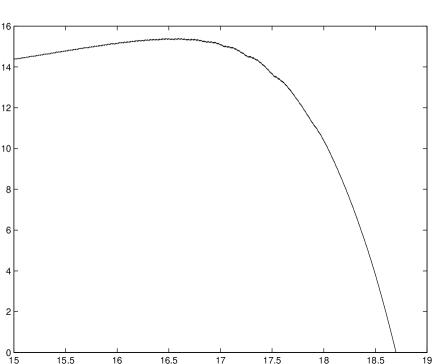
Figure 9: Scaling constant in time for the fitting $\|\omega\|_{\infty}\approx c/(T-t)$, $T=18.7$.

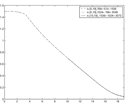
Figure 10: The inverse of maximum vorticity $\|\omega\|_{\infty}$ in time using different resolutions.

4.4 Velocity profile

One of the important findings of our computations is that the velocity field is actually bounded by 1/2 up to $T=19$. This is in contrast to Kerr’s computations in which the maximum velocity was shown to blow up like $O(T-t)^{-1/2}$. We plot the maximum velocity as a function of time using different resolutions in Figure 11. The computation with the resolution $768\times 512\times 1536$ shows some mild discrepancy toward the end of the computation. On the other hand, the computation obtained by resolution $1024\times 768\times 2048$ and the one obtained by resolution $1536\times 1024\times 3072$ are almost indistinguishable. As we can see, the maximum velocity grows slowly in time and is relatively small in magnitude. There is a relatively fast growth of maximum velocity between $t=14$ and $t=17$. But this growth becomes saturated by $t=17.5$. After $t=18.4$, the velocity experiences a mild growth, but it is still bounded by $0.46$ at the final time $T=19$. We also plot the contours of $|\vec{u}|$ near the region of maximum vorticity at $t=18$ and $19$ in Figure 12. As we can see, the velocity seems to be well resolved.

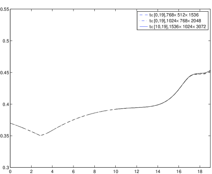
Figure 11: Maximum velocity $\|\vec{u}\|_{\infty}$ in time using different resolutions.

The fact that the velocity field is bounded is significant. By re-examining the non-blowup conditions of the theory of Deng-Hou-Yu [9], we find that the first condition is now satisfied with $\alpha=0$ since the velocity field is bounded. According to [17], we have $\max_{L_{t}}(|\kappa|,\;|\nabla\cdot\vec{\xi}|)\leq C_{0}(T-t)^{-1/2}$. In fact, our computations indicate that the curvature and the divergence of the unit vorticity vector are actually bounded. With $\alpha=0$, we can now choose the vortex line segment of length, $L(t)=(T-t)^{\beta}$ with $\beta=1/2<1-\alpha$, so that the second condition is now satisfied. Thus, the theory of Deng-Hou-Yu applies, which implies non-blowup of the 3D Euler equations up to $T$.

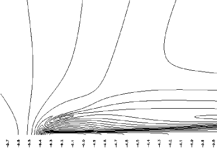
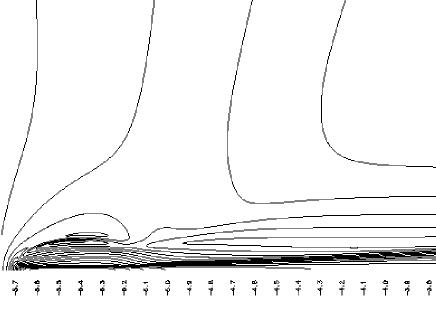
Figure 12: The contour of $|\vec{u}|$ in the region of maximum vorticity on the symmetry plane. The pictures are plotted at $t=18$ and $t=19$ respectively using resolution $1536\times 1024\times 3072$.

4.5 Local vorticity structure

In this subsection, we would like to examine the local vorticity structure near the region of the maximum vorticity. To illustrate the development in the symmetry plane, we show a series of vorticity contours near the region of the maximum vorticity at late times in a manner similar to the results presented in [14]. In Kerr’s computations, he observed that the head and tail in the symmetry plane develop a corner separating the head and tail. We adopt Kerr’s definition of the “head” to be the region extending above the vorticity peak $\omega_{p}$ just behind the leading edge of the vortex sheet. The “tail” is the vortex sheet extending behind the peak vorticity. One interesting question is to determine whether one direction becomes progressively more flattened or stretched as the flow evolves and whether the rates of collapse are the same in different directions. Our computational results are in qualitative agreement with Kerr’s in the early and intermediate stages. In particular, we observe that as the flow evolves the region of peak vorticity concentrates into the region where the vortex sheets of the head and tail meet. To compare with Kerr’s figures, we scale the vorticity contours in the $x-z$ plane by a factor of 5 in the $z$ direction. The results at $t=15$ and $t=17$ are plotted in Figure 13. We can see that the location of maximum axial vorticity moves toward the corner where the vortex sheets of the head and tail meet as time increases, see also Figure 14. This is in qualitative agreement with Kerr’s results.

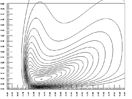
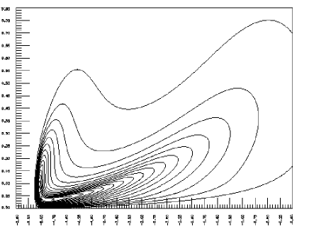
Figure 13: The contour of axial vorticity around the maximum vorticity on the symmetry plane at $t=15,17$. The figure is scaled in $z$ direction by a factor of $5$ to compare with the Figure 4 in [14]. A contour at value very close to the maximum value is plotted to show the location of the maximum vorticity.

In order to see better the dynamic development of the local vortex structure, we plot a sequence of vorticity contours on the symmetry plane at $t=16,17,18,$ and $19$ respectively in Figure 14. The pictures are plotted using the original length scales, without the scaling by a factor of 5 in the $z$ direction as in Figure 13. From these results, we can see that the vortex sheet is compressed in the $z$ direction. It is clear that a thin layer (or a vortex sheet) is formed dynamically. The head of the vortex sheet is a bit thicker than the tail at the beginning. The head of the vortex sheet begins to roll up around $t=16$. By the time $t=19$, the head of the vortex sheet has traveled backward for quite a distance, and the vortex sheet has been compressed quite strongly along the $z$ direction.

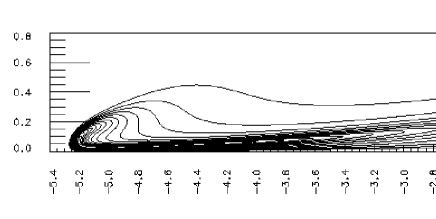
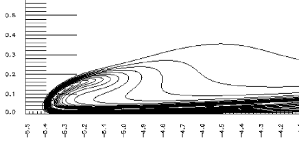
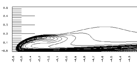
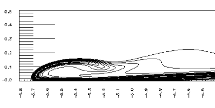
Figure 14: The contour of axial vorticity around the maximum vorticity on the symmetry plane at $t=17.5,18,18.5,19$.

We also plot the isosurface of vorticity near the region of the maximum vorticity in Figures 15 and 16 to illustrate the dynamic roll-up of the vortex sheet near the region of the maximum vorticity. Figure 15 gives the local vorticity structure at $t=17$. If we scale the local roll-up region on the left hand side next to the box by a factor of 4 along the $z$ direction, as was done in [17], we would obtain a local roll-up structure which is qualitatively similar to Figure 1 in [17]. In Figure 16, we show the local vorticity structure for $t=18$ and $19$. In both figures, the isosurface is set at $0.5\times\|\vec{\omega}\|_{\infty}$. Here we make a few observations. First, the vortex lines near the region of maximum vorticity are relatively straight and the vorticity vectors seem to be quite regular. This was also observed in [14]. On the other hand, the inner region containing the maximum vorticity does not seem to shrink to zero at a rate of $(T-t)^{1/2}$, as predicted in [14]. The length and the width of the vortex sheet are still $O(1)$, although the thickness of the vortex sheet becomes quite small.

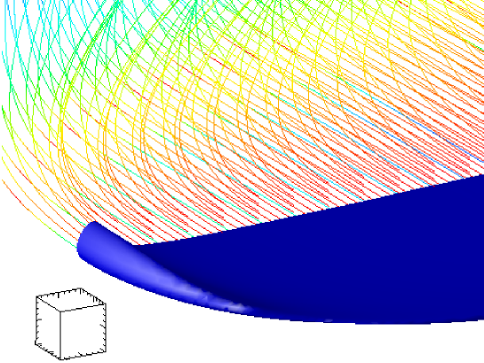
Figure 15: The local 3D vortex structure and vortex lines around the maximum vorticity at $t=17$. The size of the box on the left is $0.075^{3}$ to demonstrate the scale of the picture.

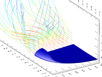
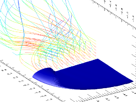
Figure 16: The local 3D vortex structures and vortex lines around the maximum vorticity at $t=18$ (on the left) and $t=19$ (on the right).

We also plot the energy spectrum in Figure 17 at $t=16,17,18,19$. A finite time blow-up of enstrophy would imply that the energy spectrum decays no faster than $|k|^{-3}$. In [14], Kerr observed that the energy spectrum decays exactly like $|k|^{-3}$, suggesting a finite time blow-up of the enstrophy (recall that enstrophy is defined as the square of the $L^{2}$ norm of vorticity, i.e. $\|\vec{\omega}\|_{2}^{2}$). Our computations show that the energy spectrum approaches $|k|^{-3}$ for $|k|\leq 100$ as time increases to $t=19$. This is in qualitative agreement with Kerr’s results. Note that there are only less than 100 modes available along the $|k_{x}|$ or $|k_{y}|$ direction in Kerr’s computations, see Figure 18 (a)-(b) of [14]. On the other hand, our computations show that the high frequency Fourier spectrum for $100\leq|k|\leq 1300$ decays much faster than $|k|^{-3}$, as one can see from Figures 17 and 23. This indicates that there is no blow-up in enstrophy. This is also supported by the enstrophy spectrum, given in Figure 18, and the plot of enstrophy as a function of time in Figures 19. In Figure 20, we plot the enstrophy production rate, which is defined as the time derivative of enstrophy. Although it grows relatively fast, it actually grows slower than double exponential in time (see the picture on the right in Figure 20). In the double logarithm plot of the enstrophy production rate, we multiply the enstrophy production rate by a constant factor 8 to make the second logarithm well-defined. It is interesting to note that the double logarithm of enstrophy production rate in Figure 20 is qualitatively similar to the double logarithm of $||\vec{\omega}||_{\infty}$ in Figure 7.

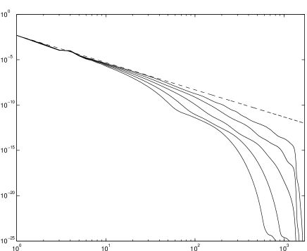
Figure 17: The energy spectra for velocity at different times in log-log scale. The energy spectrum is calculated using $E(k)=\sum_{|\vec{k}|\in(k-1/2,k+1/2]}|\widehat{u}_{\vec{k}}|^{2}$. The time for the spectral lines from bottom to top are $t=15,16,17,18,19$. The dashed line corresponds to $k^{-3}$.

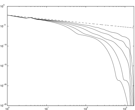
Figure 18: The enstrophy spectra for vorticity at different times in log-log scale. The enstrophy spectrum is calculated using $Ens(k)=\sum_{|\vec{k}|\in(k-1/2,k+1/2]}|\widehat{\omega}_{\vec{k}}|^{2}$. The dashed line corresponds to $k^{-1}$.

Figure 19: The enstrophy as a function of time, resolution $1536\times 1024\times 3072$.

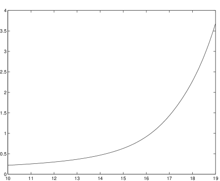
Figure 20: The enstrophy production rate (left) and the double logarithm of 8 times enstrophy production rate (right) as a function of time, resolution $1536\times 1024\times 3072$.

4.6 Resolution Study

In this subsection, we perform a resolution study to make sure that the nearly singular behavior of the 3D Euler equations is resolved by our computational grid. In Figure 6, we have performed resolution study for the maximum vorticity using three different resolutions and found very good agreement for the time interval $[0,18]$. There is only a mild disagreement toward the end of the computations from $t=18$ to 19. In our computations with different resolutions, we find that the maximum vorticity always grows slower than double exponential in time. Similar resolution study has been performed for the inverse of maximum vorticity in Figure 10 and for the maximum velocity in Figure 11. We observe excellent agreement between the solutions obtained by the two largest resolutions. We have also performed similar resolution study in the Fourier space by examining the convergence of the energy and enstrophy spectra using different resolutions. We observe that the Fourier spectrum corresponding to the effective modes of one resolution is in excellent agreement with that corresponding a higher resolution computation, see Figures 5, 22 and 23.

To see how many grid points we have across the most singular region, we plot the underlying mesh for the vorticity contours in the $x-z$ plane in Figure 21. One can see from this picture that we have about $16$ grid points in the $z$ direction at $t=18$ and $8$ grid points at $t=19$. It is also interesting to note that at $t=18.5$, the location of the maximum vorticity has moved away from the bottom of the vortex sheet structure. If the current trend continues, it is likely that the location of the maximum vorticity will continue to move away from the bottom of the vortex sheet. One of the possible blow-up scenarios is that the interaction of the two perturbed antiparallel vortex tubes would induce a strong compression between the two vortex tubes, leading to a finite time collapse of the two vortex tubes. The fact that the location of the maximum vorticity moves away from the dividing plane of the two vortex tubes seems to destroy the desired mechanism to produce a blow-up.

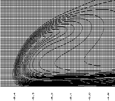
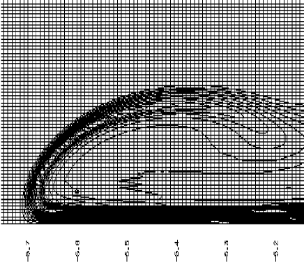
Figure 21: This picture is to illustrate the mesh around the maximum vorticity. The times for this plot are $18,19$. At $t=19$, we still have about $8$ points along $z$ direction to resolve the nearly singular layer.

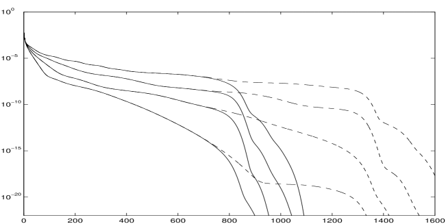
Figure 22: Convergence study for enstrophy spectra using different resolutions. The dashed lines and the solid lines are the enstrophy spectra on resolution $1536\times 1024\times 3072$ and $1024\times 768\times 2048$, respectively. The times for the lines from bottom to top are $t=16,17,18,19$.

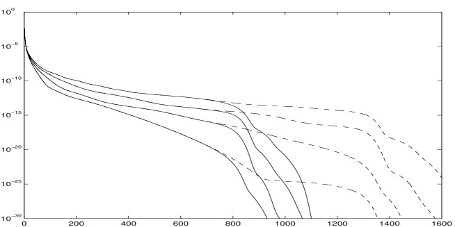
Figure 23: Convergence study for energy spectra using different resolutions. The dashed lines and the solid lines are the energy spectra on resolution $1536\times 1024\times 3072$ and $1024\times 768\times 2048$, respectively. The times for the lines from bottom to top are $t=16,17,18,19$.

5 Concluding Remarks

We investigate the interaction of two perturbed vortex tubes for the 3D Euler equations using Kerr’s initial data. Our numerical computations demonstrate a very subtle dynamic depletion of vortex stretching. The maximum vorticity is shown to grow no faster than double exponential in time up to $T=19$, beyond the singularity time predicted by Kerr in [14]. The local geometric regularity of vortex lines seems to be responsible for this dynamic depletion of vortex stretching. Sufficient numerical resolution is essential in capturing the double exponential growth in vorticity and the dynamic depletion of vortex stretching. The velocity field and the enstrophy are shown to be bounded throughout the computations. We provide evidence that the vortex stretching term is only weakly nonlinear and is bounded by $\|\vec{\omega}\|_{\infty}\log(\|\vec{\omega}\|_{\infty})$. Such an upper bound on the vortex stretching term implies that the maximum vorticity is bounded by the double exponential in time. Our computational results also satisfy the non-blowup conditions of Deng-Hou-Yu, which provides a theoretical support for our computational results.

The current computations, even with this level of resolution, can not rule out the possibility of the blow-up of the 3D Euler equations for large times for Kerr’s initial data. The theoretical results of [8, 9, 10] and the computations presented here suggest that a finite time singularity, if it exists, would have rather complicated geometric structures. There are other types of potential Euler singularities that are not considered in this paper. Among them, the Kida-Pelz initial condition [3, 21] is worth further investigation. The extra symmetry constraints in this type of initial data are believed to be important in producing a finite time singularity for the 3D Euler equations. Indeed, the computations by Boratav and Pelz [3] and Pelz [21] indicate a more singular self-similar type of blow-up. Pelz’s computations also fall in the critical case of the non-blowup theory of Deng-Hou-Yu [9, 10]. We are currently investigating this problem numerically using even higher resolutions. We will report the results elsewhere.

Appendix. Corrections to Some Misprints in [14]

In this appendix, we explain the corrections that we make regarding the misprints in the description of the initial condition in [14]. There are two constraints on the initial vorticity. The first one is that it must be divergence free. The second one is that it must satisfy the periodic boundary condition. It is obvious that we have

$$\nabla\cdot(\omega_{x},\;\omega_{y},\;\omega_{z})=0.$$ (17)

Thus the divergence free constraint on the initial vorticity implies that $\omega(r)$ must satisfy

$$\nabla\omega(r)\cdot(\omega_{x},\;\omega_{y},\;\omega_{z})=0.$$

The analytic expression of the initial vorticity profile in [14] does not satisfy the above constraint due to a few typos in various formula. We correct these typos by comparing the analytic formula with the formula that were actually used by Kerr in his Fortran subroutine that generates the initial data. Below we would list these typos and point out the corrections.

1. In equation (7), the original expression in [14] was written as $[x_{0}+x(s),y,z_{0}+z(s)]$. We remove $x_{0}$ and $z_{0}$ from (7) since the definition of $x(s)$ and $z(s)$ has already taken $x_{0}$ and $z_{0}$ into account.

2. In (8), the original expression in [14] was given as $x_{0}+\delta_{x}\cos(s)$. This would violate the divergence free condition. We correct this by replacing $\cos(s)$ with $\cos\left(\pi s/L_{x}\right)$.

3. In (9), the original expression was $z_{0}+\delta_{z}\cos(s)$. This again violates the divergence free condition. We correct it by replacing $\cos(s)$ with $\cos\left(\pi s/L_{z}\right)$.

4. In (12), the last factor in the original expression was $\sin(\pi s(y))$. We correct it by replacing $\sin(\pi s(y))$ with $\sin\left(\pi s(y)/L_{x}\right)$.

5. In (14), the last factor in the original expression was $\sin(\pi s(y))$. We correct it by replacing $\sin(\pi s(y))$ with $\sin\left(\pi s(y)/L_{z}\right)$.

With the above corrections, it can be verified that both the divergence free condition and the periodic boundary conditions are satisfied.

Based on Kerr’s subroutine that generates the initial data, we also make one minor modification in the definition of $f(r)$. The original equation in [14] for (5) was given by

$$f(r)=\frac{-r^{2}}{1-r^{2}}+r^{2}\left(1+r^{2}+r^{4}\right).$$ (18)

After studying Kerr’s code, we found that the function $f(r)$ in his code was actually defined using (5) instead of the above formula. The difference lies in the first factor in the second term of the above equation. What was used in Kerr’s code was $r^{4}$ instead $r^{2}$ in the above equation. This minor modification has little effect on the behavior of the solution from our computational experience. We make this minor modification to $f(r)$ in order to match exactly the initial condition that was actually used in Kerr’s computations.

Acknowledgments. We would like to thank Prof. Lin-Bo Zhang from the Institute of Computational Mathematics in Chinese Academy of Sciences (CAS) for providing us with the computing resource to perform this large scale computational project. Additional computing resource was provided by the Center of High Performance Computing in CAS. We also thank Prof. Robert Kerr for providing us with his Fortran subroutine that generates his initial data. This work was in part supported by NSF under the NSF FRG grant DMS-0353838 and ITR Grant ACI-0204932. Part of this work was done while Hou visited the Academy of Systems and Mathematical Sciences of CAS in the summer of 2005 as a member of the Oversea Outstanding Research Team for Complex Systems. Finally, we would like to thank Profs. Hector Ceniceros and Robert Kerr for their valuable comments on the original manuscript.

References

- [1] C. Anderson and C. Greengard, The vortex ring merger problem at infinite reynolds number, Comm. Pure Appl. Maths 42 (1989), 1123.
- [2] J. T. Beale, T. Kato, and A. Majda, Remarks on the breakdown of smooth solutions of the 3-D Euler equations, Comm. Math. Phys. 96 (1984), 61–66.
- [3] O. N. Boratav and R. B. Pelz, Direct numerical simulation of transition to turbulence from a high-symmetry initial condition, Phys. Fluids 6 (1994), no. 8, 2757–2784.
- [4] O. N. Boratav, R. B. Pelz, and N. J. Zabusky, Reconnection in orthogonally interacting vortex tubes: Direct numerical simulations and quantifications, Phys. Fluids A 4 (1992), no. 3, 581–605.
- [5] R. Caflisch, Singularity formation for complex solutions of the 3D incompressible Euler equations, Physica D 67 (1993), 1–18.
- [6] A. Chorin, The evolution of a turbulent vortex, Commun. Math. Phys. 83 (1982), 517.
- [7] P. Constantin, Geometric statistics in turbulence, SIAM Review 36 (1994), 73.
- [8] P. Constantin, C. Fefferman, and A. Majda, Geometric constraints on potentially singular solutions for the 3-D Euler equation, Commun. in PDEs. 21 (1996), 559–571.
- [9] J. Deng, T. Y. Hou, and X. Yu, Geometric properties and non-blowup of 3-D incompressible Euler flow, Comm. in PDEs. 30 (2005), no. 1, 225–243.
- [10] , Improved geometric conditions for non-blowup of 3D incompressible Euler equation, accepted by Comm. in PDEs. (2005).
- [11] D. G. Ebin, A. E. Fischer, and J.E. Marsden, Diffeomorphism groups, hydrodynamics and relativity, The 13th Biennial Seminar of Canadian Mathematical Congress (J. Vanstone, ed.), 1970, pp. 135–279.
- [12] R. Grauer, C. Marliani, and K. Germaschewski, Adaptive mesh refinement for singular solutions of the incompressible Euler equations, Phys. Rev. Lett. 80 (1998), 19.
- [13] R. Grauer and T. Sideris, Numerical computation of three dimensional incompressible ideal fluids with swirl, Phys. Rev. Lett. 67 (1991), 3511.
- [14] R. M. Kerr, Evidence for a singularity of the three dimensional, incompressible Euler equations, Phys. Fluids 5 (1993), no. 7, 1725–1746.
- [15] , Euler singularities and turbulence, 19th ICTAM Kyoto ’96 (T. Tatsumi, E. Watanabe, and T. Kambe, eds.), Elsevier Science, 1997, pp. 57–70.
- [16] , The outer regions in singular Euler, Fundamental problematic issues in turbulence (Birkhäuser) (Tsnober and Gyr, eds.), 1999.
- [17] , Velocity and scaling of collapsing Euler vortices, Phys. Fluids (to appear).
- [18] R. M. Kerr and F. Hussain, Simulation of vortex reconnection, Physica D 37 (1989), 474.
- [19] A. J. Majda and A. L. Bertozzi, Vorticity and Incompressible Flow, Cambridge University Press, 2002.
- [20] M. V. Melander and F. Hussain, Cross linking of two antiparallel vortex tubes, Phys. Fluids A (1989), 633–636.
- [21] R. B. Pelz, Locally self-similar, finite-time collapse in a high-symmetry vortex filament model, Phys. Rev. E 55 (1997), no. 2, 1617–1626.
- [22] A. Pumir and E. E. Siggia, Collapsing solutions to the 3-D Euler equations, Phys. Fluids A 2 (1990), 220–241.
- [23] M. J. Shelley, D. I. Meiron, and S. A. Orszag, Dynamical aspects of vortex reconnection of perturbed anti-parallel vortex tubes, J. Fluid Mech. 246 (1993), 613–652.
- [24] P. Stinis and A. Chorin, Numerical scaling analysis of the small-scale structure in turbulence, LBNL report LBNL-59490, Mathematics Dept. (2006).