Swimming in curved space
or
The Baron and the cat

Abstract

We study the swimming of non-relativistic deformable bodies in (empty) static curved spaces. We focus on the case where the ambient geometry allows for rigid body motions. In this case the swimming equations turn out to be geometric. For a small swimmer, the swimming distance in one stroke is determined by the Riemann curvature times certain moments of the swimmer.

1 Introduction

Every street cat can fall on its feet [3, 6, 8, 10] but only Baron von Munchausen ever claimed to have lifted himself by applying self-forces (actually, by pulling on his hair [11]). The reason why none else does is because, as we were taught in high-school physics, the motion of the center of mass can not be affected by internal forces. In particular, if the center of mass is at rest, it can only be moved by external forces. As pointed out by J. Wisdom [2, 13], in a curved space this piece of high school physics is no longer true: A deformable body can apply internal forces that would result in swimming, much like a cat turning in Euclidean space while maintaining zero angular momentum [6].

The reason why high school physics fails for curved space is tied to the fact that the notion of center of mass is a fundamentally a Euclidean notion, with no analog in curved space, see Fig. 1.

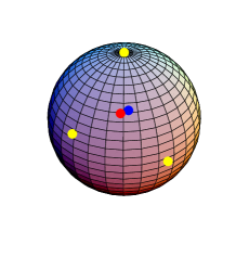
Figure 1: The red dot is equidistant from the three identical yellow point masses and so is one natural notion of a center of mass. The blue dot is another center of mass. It is obtained by first moving the pair of points masses on the right to their center of mass and then finding the center of mass of the remaining pair of (unequal) masses.

Swimming is the motion of deformable bodies. More precisely, we shall mean by this the rigid body motion affected by a periodic deformation. After completing a swimming stroke the swimmer regains its original shape and finds itself in a different location. The new location is determined by solving the equations of motion [12].

In a generic curved space, the shape of a general swimmer completely determines its location. Therefore a strictly periodic deformation allows the swimmer merely to wriggle. To be able to swim anywhere and with arbitrary orientation the ambient space must be homogeneous and isotropic. This is the case for the Euclidean space, and also for symmetric spaces such as spheres and hyperbolic spaces. As we shall see, swimming in such spaces is geometric.

Swimming in more general curved spaces that do not necessarily allow for rigid body motions require the replacement of shape space by a different space of controls. Here we shall focus on the considerably simpler case where the ambient space allows for rigid body motions.

What do we mean by swimming? Swimming is associated with the translation bit of a rigid body motion. Recall that even in a Euclidean space splitting the translations from the rotation for a given rigid body motion requires picking a fiducial point [7]. If we let a turning cat pick the tip of its tail as a favorite fiducial point it may claim to be Baron von Munchausen since turning about its center of mass is equivalent to turning about the tip of the tail accompanied by translation. The cat is not really swimming because in Euclidean space swimming is defined as the the translation of the center of mass. Since in a curved space there is no natural notion of a center of mass we need to specify what does one mean by swimming. We shall call swimming a motion that after the completion of a stroke, results in a rigid body motion that does not leave any point inside the swimmer fixed.

Rigid body motions are generated by the isometries of space. These are represented by Killing vector fields which we shall denote by $\xi_{\beta}(x)$. There are $k={d+1\choose 2}$ such fields in $d$ dimensional maximally symmetric spaces. A natural notion of translations is associated with those Killing fields that reduce to the Euclidean translations at some fiducial point of the swimmer. If the swimmer is sufficiently small relative to the length scale given by the curvature, the Killing fields associated with these translations will not vanish near the swimmer. This means that no point of the swimmer is stationary under the rigid motion generated by such Killing fields and gives a natural notion of swimming.

As we shall see, a deformable body can generate a rigid body motion associated to the Killing field $\xi$, if the two-form $d\xi$ is non-zero near the swimmer. Thus, for example, a cat can turn in Euclidean space because the Killing two forms associated to rotations do not vanish. The Baron, in contrast, must be lying because the Killing two forms associated to translations in Euclidean space vanish identically. In a curved space any rigid body motion becomes possible because, in general, none of the Killing two forms vanish identically. Since the Killing two-forms associated to translation are proportional to the Riemann curvature swimming in a curved space is proportional to the Riemann curvature.

We shall restrict ourselves to studying non-relativistic swimmers so that the swimming problem reduces to a problem in Newtonian mechanics on a given static curved space. This is a simplified version of the problem of the motion of extended bodies in general relativity which is notoriously difficult [4].

Our two main results are Eq. (4.7) and Eq. (6.1). The first gives the swimming distance of a small swimmer performing an infinitesimal stroke generated by any pair of deformations. The second is the special case of linear deformations. In this case, the swimming distance is proportional to the Riemann curvature and certain moments of the swimmer. The overall structure of the formulas is similar to the formula written by Wisdom [13] although both the setting, the details and the consequences are different.

2 Swimming from conservation laws

2.1 Constants of motion: Nöther theorem

Consider a body made of a collection of $N$ particles with mass $m_{n}$ located at generalized coordinates $x_{n}$, with $n=1,\dots N$. Let $L(\dot{x},x,t)$ denote the (time-dependent) Lagrangian of the system which admits a symmetry associated with the Killing field $\xi(x)$, i.e. $L$ is invariant under the shift $x\to x+\varepsilon\xi(x)$. The symmetry implies the conservation of

$$P_{\xi}=\sum_{n}\left(\frac{\partial L}{\partial\dot{x}_{n}^{i}}\right)\,\xi^{i}(x_{n})\,.$$ (2.1)

Indeed the symmetry of the Lagrangian and the Euler-Lagrange equations of motions imply:

$$0=\frac{\partial L}{\partial\varepsilon}=\sum_{n}\left(\frac{\partial L}{\partial\dot{x}_{n}}\,\dot{\xi}(x_{n})+\frac{\partial L}{\partial x_{n}}\,\xi(x_{n})\right)=\frac{dP_{\xi}}{dt}$$ (2.2)

Suppose the dynamics takes place on manifold with metric $g$. The (time dependent) Lagrangian, being the difference of the non-relativistic kinetic energy and the potential energy, is:

$$L=\frac{1}{2}\sum_{n}m_{n}\,\dot{x}_{n}\cdot\dot{x}_{n}-\sum_{pairs}V_{mn}\big{(}dis(x_{n},x_{m}),t\big{)}$$ (2.3)

The Lagrangian is invariant under isometries of the manifold. The potential energy, being a function of the relative distances, guarantees Newton third law: The force that particle $a$ applies on $b$ is directed along the geodesic separating the two and is opposite and equal to the force that $b$ applies on $a$.

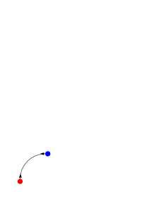
Figure 2: Newton third law in curved space: The mutual forces are directed along a geodesic and are balanced.

The constant of motion $P_{\xi}$, associated to the isometry $\xi$, is independent of $V$ and is given by

$$P_{\xi}=\sum_{n}m_{n}\,\dot{x}_{n}\cdot\,\xi(x_{n})$$ (2.4)

We shall assume throughout that the particles that make up the body are initially at rest, $\dot{x}_{n}=0$, and so $P_{\xi}=0$.

Suppose now that the body, initially at rest, can control its shape by, for example, controlling $V$. The rigid body part of the resulting motion is determined by the conservations laws

$$\sum_{n}m_{n}\,\xi_{(\beta)}(x_{n})\cdot dx_{n}=0,\quad\beta=1\dots,k$$ (2.5)

It is evident that the resulting rigid body motion is geometric in the sense that the time parametrization disappeared.

3 Deformations and rigid body motions

We want to describe the (infinitesimal) motion of a deformable body as a combination of an (infinitesimal) deformation and rigid body motion. We write the infinitesimal displacement of the n-th point mass in the form

$${dx_{n}}^{j}={\xi_{(\beta)}}^{j}(x_{n})\,\kern-1.00006pt{\raise 3.44444pt\hbox{ -}}\kern-6.00006pt{d}\tau^{(\beta)}+{\eta_{(b)}}^{j}(x_{n})\,d\sigma^{(b)}\,,$$ (3.1)

where $\xi_{(\beta)}\,\beta=1,\dots,k$ are Killing fields that generate rigid body motions and $\eta_{(b)}(x),\ b=1,\dots\ell$ are deformation vector fields that do not. The Killing fields satisfy the Killing equation [14]

$$\nabla_{(j}\xi_{k)}=\nabla_{j}\xi_{k}+\nabla_{k}\xi_{j}=0$$ (3.2)

which can be interpreted as the statement that rigid body motion induces no strain. The deformation fields, in contrast, induce a non-vanishing strain

$$du_{jk}=\big{(}\nabla_{j}\,\eta^{(b)}_{k}+\nabla_{k}\,\eta^{(b)}_{j}\big{)}d\sigma_{b}$$ (3.3)

We may then think of $d\sigma_{b}$ as the infinitesimal coordinates of the swimmer’s control space.

Substituting Eq. (3.1) in Eq. (2.5) yields $k$ linear relations between the infinitesimal rigid body motion $\kern-1.00006pt{\raise 3.44444pt\hbox{ -}}\kern-6.00006pt{d}\tau$ and the infinitesimal deformations $d\sigma$. These will turn out to be the swimming equations. However, to derive these we first need to put coordinates on shapes and rigid motions that will effectively replace the possibly very large number of particle coordinates $x_{n}$.

3.1 Coordinates for rigid body location

Let $\tau=0$ denote the initial location of the swimmer, the shape $S(0)$. We may identify $\tau\in\mathbb{R}^{k}$ as the new location of the swimmer (shape) that underwent rigid body motion from the origin. More precisely, the flow

$$\dot{x}^{j}_{t}=\tau\cdot\xi^{j}(x_{t})=\tau^{\alpha}\,{\xi_{\alpha}}^{j}(x_{t})$$ (3.4)

at one unit of time gives the displaced shape. For small $\tau$ the mapping $x\to x_{\tau}$ is given by

$$x^{j}_{\tau}=x^{j}+\tau^{\alpha}{\xi_{\alpha}}^{j}(x)+\mbox{$1\over 2$}\,\tau^{\alpha}\tau^{\beta}\,{\xi_{\alpha}}^{i}\partial_{i}{\xi_{\beta}}^{j}+\dots$$ (3.5)

We write for the displaced shape $S(\tau)$, symbolically,

$$S(\tau)=e^{\tau\cdot\xi}S(0)\,.$$ (3.6)

3.2 Shape coordinates

We now want to put coordinates on shape space. Let $\sigma=0$ denote the undeformed shape $S(0)$. The deformed shape, without paying attention to its location, will be denote by $S(\sigma)$ with $\sigma\in\mathbb{R}^{\ell}$ and $\ell$ being the number of independent strain (deformation) fields at the disposal of the swimmer. More precisely, the deformed shape is covariantly defined by the solution of the flow

$$\dot{x}^{j}_{t}=\sigma\cdot\eta^{j}(x_{t})$$ (3.7)

after a unit time. For small $\sigma$ the mapping $x\to x_{\sigma}$ is given by

$$x_{\sigma}^{j}=x^{j}+\sigma^{b}{\eta_{(b)}}^{j}(x)+\frac{1}{2}\sigma^{b}\sigma^{c}\,{\eta_{(b)}}^{k}(x)\,\partial_{k}{\eta_{(c)}}^{j}(x)+\dots$$ (3.8)

We write the corresponding map of the shape, formally,

$$S(\sigma)=e^{\sigma\cdot\eta}S(0)$$ (3.9)

Note that this is not the physical evolution, since the latter will be accompanied by a rigid motion.

3.3 Shape and position coordinates

The shape and location can be parameterized as by a pair $(\sigma,\tau),\ \tau\in\mathbb{R}^{k},\ \sigma\in\mathbb{R}^{\ell}$. $\sigma$ is the deformation coordinate and $\tau$ the location coordinate. Since deformations do not commute with rigid motions in general, to assign a pair $(\sigma,\tau)$, we need to choose an order. A natural choice, which reflects the interpretation that the rigid motion is a consequence of the deformation, is to take $S(\tau,\sigma)$ to mean

$$S(\sigma,\tau)=e^{\tau\cdot\xi}\,e^{\sigma\cdot\eta}\,S(0)$$ (3.10)

$e^{\sigma\cdot\eta}$ takes $S(0)$ to $S(\sigma,0)$. By convention $S(\sigma,0)$ has the same location coordinate $\tau$ as the $S(0)$. $e^{\tau\cdot\xi}$ is the rigid motion by $\tau$ to the correct physical location.

3.4 Gauge condition

A swimmer may be able to control its internal stress and thereby its internal strain, but not directly the deformation fields $\eta$. This reflects the simple fact that there is no canonical way to integrate Eq. (3.3) to pair a deformation field with a strain since there is ambiguity in the Killing fields. To pick a unique $\eta$ one needs to impose $k$ gauge conditions. To do so it is convenient to introduce a notion of scalar product for extended bodies.

Given a body made of a collection of point particles with masses $m_{n}$ at locations $x_{n}$ we define a scalar product of two vector fields $u,v$ by:

$$\langle u|v\rangle=\frac{1}{M}\sum_{n}m_{n}\,u_{j}(x_{n})\,v^{j}(x_{n}),\quad M=\sum m_{n}\,.$$ (3.11)

We pick the gauge where each deformation field $\eta$ is orthogonal to all the Killing fields:

$$\langle\xi_{\alpha}|\eta\rangle=0\,,\quad\alpha=1,\dots,k\,.$$ (3.12)

This gauge will play a role in obtaining simple expression for swimming.

4 The swimming equations

4.1 Covariant description of swimming

In this subsection we calculate the translation $\Delta\tau$ associated with a small loop $\sigma(t)$ near the origin of shape space. Applying the deformation forces the particles making up the body to move along certain trajectories $x_{n}(t)$. At the leading order one has by Eqs. (3.5,3.8) simply

$$dx^{j}_{n}=\xi^{j}_{(\alpha)}\,d\tau^{(\alpha)}+\eta_{(b)}^{j}d\sigma^{(b)}+O(\sigma d\sigma),\quad\xi^{j}_{(\beta)}\big{(}x_{n}(t)\big{)}=\xi^{j}_{(\beta)}+O(\sigma),$$ (4.1)

and the rhs of both equations is evaluated at $x_{n}(0)$. Substituting in the conservation law (2.5) we find a relation between the differential rigid motion, $\kern-1.00006pt{\raise 3.44444pt\hbox{ -}}\kern-6.00006pt{d}\tau$, and the differential of the strain, $d\sigma$:

$$\langle\xi_{(\beta)}|\xi_{(\alpha)}\rangle\,\kern-1.00006pt{\raise 3.44444pt\hbox{ -}}\kern-6.00006pt{d}\tau^{(\alpha)}+\langle\xi_{(\beta)}|\eta_{(b)}\rangle\,d\sigma^{(b)}=O(\sigma d\sigma),\quad\beta=1,...k.$$ (4.2)

The gauge condition (3.12) is now seen to imply (in fact is equivalent to the statement) that $d\tau=O(\sigma d\sigma)$ i.e. that $\tau=O(\sigma^{2})$. Using this and equations Eqs. (3.5,3.8) again we see that to the next order in $\sigma$

$$dx^{j}_{n}={\xi_{(\alpha)}}^{j}\,\kern-1.00006pt{\raise 3.44444pt\hbox{ -}}\kern-6.00006pt{d}\tau^{\alpha}+{\eta_{(b)}}^{j}d\sigma^{b}+\frac{1}{2}\,d(\sigma^{b}\,\sigma^{c})\,\eta_{(c)}^{k}\partial_{k}\eta_{(b)}^{j}\Big{|}_{x_{n}}+O(\sigma^{2}d\sigma)$$ (4.3)

$$\xi^{j}_{(\beta)}\big{(}x_{n}(t)\big{)}=\xi^{j}_{(\beta)}+\sigma^{c}\,{\eta_{(c)}}^{k}\partial_{k}\xi^{j}_{(\beta)}\Big{|}_{x_{n}}+O(\sigma^{2})$$ (4.4)

Substituting these two equations in the conservation law (2.5) (and again using (3.12)) we find

$$\langle\xi_{(\beta)}|\xi_{(\alpha)}\rangle\,\kern-1.00006pt{\raise 3.44444pt\hbox{ -}}\kern-6.00006pt{d}\tau^{\alpha}+\langle\partial_{k}{\xi_{(\beta)}}_{j}|{\eta^{k}_{(c)}}\,{\eta^{j}_{(b)}}\rangle\,\sigma^{c}\,d\sigma^{b}+\frac{1}{2}\,\langle{\xi_{(\beta)}}_{j}|\eta_{(c)}^{k}\,\partial_{k}{\eta^{j}_{(b)}}\rangle\,d(\sigma^{b}\,\sigma^{c})=O(\sigma^{2}d\sigma)$$

where the brackets are evaluated for the undeformed body, (and so are constants, independent of $\sigma$ and $\tau$). The holonomy follows by applying the $d$ operation. Since $d(\sigma^{b}\sigma^{c})$ is closed, it is annihilated by $d$ and the holonomy $\delta\tau=d\kern-1.00006pt{\raise 3.44444pt\hbox{ -}}\kern-6.00006pt{d}\tau$ of an infinitesimal cycle of strains is determined by the linear system of equations:

$$\langle\xi_{(\beta)}|\xi_{(\alpha)}\rangle\,\delta\tau^{\alpha}+\langle\partial_{k}\xi_{(\beta)j}|\eta_{(c)}^{k}\,\eta_{(b)}^{j}\rangle\,d\sigma^{c}\wedge d\sigma^{b}=0\,,\quad\beta=1,\dots,k$$ (4.5)

Using the antisymmetry of forms and the freedom to relabel indices one can rewrite the second term as

$$\langle\partial_{k}\xi_{(\beta)j}|\eta_{(b)}^{k}\,\eta_{(c)}^{j}\rangle\,d\sigma^{b}\wedge d\sigma^{c} = -\langle\partial_{j}\xi_{(\beta)k}|\eta_{(b)}^{k}\,\eta_{(c)}^{j}\rangle\,d\sigma^{b}\wedge d\sigma^{c}$$ (4.6)

$$= \frac{1}{2}\langle\partial_{[k}(\xi_{\beta})_{j]}|\eta_{(b)}^{k}\,\eta_{(c)}^{j}\rangle\,d\sigma^{b}\wedge d\sigma^{c}$$

$$= \frac{1}{2}\,\langle d\xi_{\beta}|\eta_{(b)}\,\eta_{(c)}\rangle\,d\sigma^{b}\wedge d\sigma^{c}$$

$d\xi$ is the two form associated to the Killing field $\xi$. Putting all of this together we get the key result, that the Euclidean motion (the holonomy) is determined by the linear system of equations:

$$\langle\xi_{(\beta)}|\xi_{(\alpha)}\rangle\ \delta\tau^{\alpha}+\frac{1}{2}\,\langle d\xi_{(\beta)}|\eta_{(b)},\eta_{(c)}\rangle\,d\sigma^{b}\wedge d\sigma^{c}=0\,,\quad\beta=1,\dots,k$$ (4.7)

Where the Killing fields $\xi_{(\alpha)}$ and the deformation fields, $\eta_{(b)}$, satisfy the gauge condition $\langle\xi_{(\alpha)}|\eta_{(b)}\rangle=0$.

5 The Killing two form

Let $\xi_{(\alpha)}$ denotes a Killing field associated with a certain rigid body motion (e.g. translation or rotation), the question whether one can or can not swim in this direction depends on purely geometric properties of the ambient space. The answer is particularly simple if we choose the Killing fields to be mutually orthogonal: $\langle\xi_{(\beta)}|\xi_{(\alpha)}\rangle=0$ for $\alpha\neq\beta$. From Eq. (4.7) we see that a rigid motion generated by $\xi_{(\alpha)}$ is possible only if the corresponding two-form $d\xi_{(\alpha)}$ does not vanish identically on shape space.

5.1 Killing fields in the Euclidean space

With $x^{j}$ Cartesian coordinate in a Euclidean space, the Killing (vector) fields generating translation in the k-th direction is

$$\xi_{(k)}=\partial_{k}$$ (5.1)

The corresponding one forms, $\xi_{(k)}=d{x^{k}}$ are evidently exact.

The Killing fields generating rotations in the $j-k$ plane about the origin are

$$\xi_{(jk)}=x^{j}\partial_{k}-x^{k}\partial_{j}$$ (5.2)

The corresponding one-forms are $\xi_{(jk)}=x^{j}\,d{x^{k}}-x^{k}\,d{x^{j}}$. These are not closed:

$$d\xi_{(jk)}=2dx^{j}\wedge d{x^{k}}$$ (5.3)

In Euclidean space the Killing fields of orthogonal translations are evidently orthogonal $\langle\xi_{j}|\xi_{k}\rangle=0$ for $j\neq k$. A trite calculation shows that the Killing fields corresponding to translations and rotations are mutually orthogonal, $\langle\xi_{j}|\xi_{kl}\rangle=0$, provided the rotations are about the center of mass. Similarly, the rotations about the principal axis of a body are mutually orthogonal.

Since $d\xi_{(k)}=0$ for the translations the Baron must be lying. Cats, in contrast, can turn in Euclidean space because of the non-vanishing of $d\xi_{(jk)}$.

5.2 Local Euclidean frames

By a local Euclidean coordinate system we mean a coordinate system where the metric tensor is the identity at the origin, $g_{ij}(0)=\delta_{ij}$ and the Christoffel symbols vanish there $\Gamma^{i}_{jk}(0)=0$. Such a coordinate systems always exists. (It is not unique, however, as $g_{ij}(0),\Gamma^{i}_{jk}(0)$ are unaffected by any coordinate transformation of the form $x^{\prime i}=x^{i}+O(x^{3})$, as well as by orthogonal transformations.) A local Euclidean system allows us to extend Euclidean notions, such as translations, linear deformations and a center of mass, to the slightly non-Euclidean setting. In local Euclidean coordinates, relations which hold in Euclidean geometry will typically get corrections of relative order $O(Rx^{2})$ where $R$ is the space curvature.

5.3 Moments

For a small swimmer we define the multipole moments in a local Euclidean coordinates by

$$Q^{ij\dots k}=\sum m_{n}\,x_{n}^{i}x_{n}^{j}\dots x_{n}^{k}$$ (5.4)

The moments are well defined up to terms which are smaller by order $O(R\,L^{2})$ where $L$ is the linear dimension of the swimmer. In particular, the vanishing of the first moments $Q^{j}=0$ says that the (approximate notion of) the center of mass is at the origin. This is a natural choice of the origin which we shall normally make.

5.4 The translation Killing two form in curved spaces

Swimming in a curved space is possible because the Killing fields corresponding to translations are not closed $d\xi_{(k)}\neq 0$. Here we shall explain what we mean by the Killing fields associated to translations in a curved space and calculate the leading behavior of the corresponding two form.

Let $x^{j}$ be a locally Euclidean coordinate system in the neighborhood of the origin. A Killing field $\xi$, if it exists, is uniquely determined by its value at the origin, $\xi_{i}(0)$, and its (necessarily antisymmetric) first derivative $\nabla_{[i}\xi_{j]}(0)$ there. It is natural then to associate with translation along the $k$ axis the Killing field $\xi_{(k)}$ which satisfies

$$\xi_{(k)i}(0)=\delta_{ki},\;\nabla_{[i}\xi_{(k)j]}(0)=0$$ (5.5)

Its leading behavior away from the origin can be determined by the Riemann curvature through the differential equation [14]

$$\nabla_{i}\nabla_{j}\xi_{l}=-{R_{jli}}^{h}\xi_{h}$$ (5.6)

Since $\Gamma(0)=0$, at the origin $\nabla_{i}\nabla_{j}\xi_{l}=\partial_{i}\nabla_{j}\xi_{l}$, substituting the initial data Eq. (5.5) on the right hand side and integrating, give

$$\nabla_{j}(\xi_{(k)})_{\ell}=-x^{i}R_{jlik}(0)+O(x^{2})$$ (5.7)

These are the $j-l$ components of the k-th Killing two form. These are evidently anti-symmetric in $j,l$, by the properties of the Riemann tensor. This guarantees the Killing equation $\nabla_{(i}\xi_{j)}=0$ to the leading order. In appendix B we give exact and explicit examples of such Killing fields and their two forms.

6 Small swimmers

The swimming equations take a more transparent form in a coordinate system which is approximately Euclidean near the swimmer. This requires that the swimmer be small. This is the case if its linear dimension $L$ is such that $RL^{2}\ll 1$, where $R$ is the curvature. Swimming then corresponds to the Killing fields associated with the translations described in subsection 5.4.

Let $x^{j}$ be a locally Euclidean coordinate system in the neighborhood of the swimmer. We choose the origin so the (approximate) center of mass is at the origin: $Q^{j}=0$. This guarantees that (to leading order in $L^{2}R$) the Killing fields associated to rotations and translations are mutually orthogonal and one can therefore study the translations independent of the rotations.

Let $\eta_{(b)}$ and $\eta_{(c)}$ be two deformation field satisfying the gauge conditions. An infinitesimal loop in strain space with area $d\sigma^{b}\wedge d\sigma^{c}$, will lead to swimming a distance $\delta x^{k}$ along the $k$-axis of a local Euclidean frame. Combining Eqs. (5.7,4.7) gives our main result:

$$M\delta x^{k}=R_{jlik}\,\left(\sum_{n}\,m_{n}\,x^{i}_{n}\,\eta_{(b)}^{j}\eta_{(c)}^{l}\Big{|}_{x_{n}}\right)\,d\sigma^{b}\wedge d\sigma^{c}\,,$$ (6.1)

Where $R_{jlik}$ is the Riemann curvature at the origin, is a property of the ambient space while the brackets are a property of the strained swimmer.

7 Swimming with constant strains

In a Euclidean space the $d+1\choose 2$ linear deformations

$$2\,\eta_{(jk)}=x^{j}\partial_{k}+x^{k}\partial_{j}\$$ (7.1)

generate constant strains (and thus are evidently transversal to the rigid body motions). The notion of linear deformations does not have a covariant meaning in a general curved space. However, there is an approximate notion of linear deformation associated to a local Euclidean frame which one can safely apply to small swimmers.

For a general swimmer, the linear deformations of Eq. (7.1) will fail to satisfy the gauge condition, Eq. (3.12). But, the deformation fields can be tweaked to do so, by adding Killing fields. Explicitly, suppose that that swimmer has its center of mass as the origin, $Q^{j}=0$, and pick the orientations of the Euclidean frame to be the principal frame of the swimmer with $Q^{jk}$ diagonal. The linear deformations $\eta_{(jk)}$ defined by

$$(Q^{kk}+Q^{jj})\,\eta_{(jk)}=x^{j}\,Q^{kk}\,\partial_{k}+x^{k}\,Q^{jj}\,\partial_{j}$$ (7.2)

(no summation over $j,k$), satisfy the gauge condition and induce (approximately) constant strains. Shape space may then be identified with $\mathbb{R}^{\ell}$ where $\ell={d+1\choose 2}$.

For linear deformations the bracket in Eq. (6.1) is clearly proportional to $Q^{imh}$, the tensor of cubic moments of the swimmer. Using the explicit form Eq. (7.2) for the deformation fields one may write

$$M\delta x^{k}=R_{jlik}\,Q^{imh}\,C^{jl}_{mk}(b,c)\,d\sigma^{b}\wedge d\sigma^{c}\,,$$ (7.3)

The matrix $C^{jl}_{mk}(b,c)$ is non-zero only when the four outside indices $(j,l,m,k)$ agree pairwise with the four internal indices $(b,c)=(\beta\beta^{\prime},\gamma\gamma^{\prime})$. Explicitly it is given by

$$C^{jl}_{mk}(\beta\beta^{\prime},\gamma\gamma^{\prime})={Q^{jj}Q^{ll}\over(Q^{\beta\beta}+Q^{\beta^{\prime}\beta^{\prime}})(Q^{\gamma\gamma}+Q^{\gamma^{\prime}\gamma^{\prime}})}\times\hskip 85.35826pt$$ (7.4)

$$\big{(}\delta_{m\beta}\delta_{j\beta^{\prime}}+\delta_{j\beta}\delta_{m\beta^{\prime}}\big{)}\,\big{(}\delta_{h\gamma}\delta_{l\gamma^{\prime}}+\delta_{l\gamma}\delta_{h\gamma^{\prime}}\big{)}.$$

The formula disentangles the space from the swimmer in the sense that $R_{khij}$ is only a property of space, while the second and third rank tensors $Q^{\beta\beta}\,,Q^{h\ell m}$ are properties of the swimmer. It follows that:

• The swimming distance scales like the cubic moment of the swimmer, as it must be by dimensional analysis. (Since the swimming is proportional to the curvature, and $d\sigma$ are dimensionless [13].) This implies that small swimmers are heavily penalized.

• A body which is invariant under inversion $x^{j}\to-x^{j}$ for all $j$, can not swim via linear deformations since $Q^{h\ell m}=0$.

• A needle can not swim under linear deformations and neither can a swimmer made of two point particles. This is because, by Eq. (7.2), a single deformation, $\eta_{11}$, (with $1$ the axis of the needle) satisfies the gauge condition, and at least two are needed to swim.

• At least three point particles are required to swim by linear deformations (as is also evident by other considerations).

Appendix A Topological swimmers

A.1 Swimming on a ring

One can swim even in flat space if the topology is nontrivial. A ring, being one dimensional, has no curvature. Nevertheless, a composite body at rest can displace itself by disintegrate into a pair of particles and recombining as shown in the Figure 3. The energy needed for breakup is recovered at the fusion. The net displacement is determined by the mass ratio of the two splinters. Ideally, the displacement does not require dissipation. The ability to swim in such (flat) spaces can, once again, be traced to the absence of a good notion of center of mass.

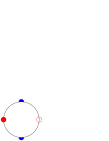
Figure 3: The full red circle on the left, splits into the two blue half balls which recombine at the empty red circle on the right. This allows for moving without violating Newton laws.

A.2 Intersecting geodesics

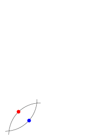
Figure 4: The red ball can displace itself to the position of the blue ball by splitting into two parts that it sends to crossing points of geodesics and then recombine satisfying Newton’s law in the process.

A variation on this theme occurs whenever the space has intersecting geodesics, as shown in Fig. 4. This mode of swimming is non-local since geodesics that start at a given point do not intersect in a small neighborhood.

A.3 Converting energy to velocity

A single particle at rest can disintegrate into a pair and recombine at a different point in such a way that the recombined particle has net velocity. Parts of the the energy needed to disintegrate is not recovered after fusion and remains as kinetic energy. This is a kinematic process that requires only contact forces and can take place even on a cone, which is everywhere flat (except at the apex) as shown in Fig. 5. The process described swimming in momentum space.

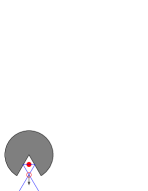
Figure 5: A cone is represented by the unshaded sector of the plane. The straight lines on the boundary of the gray area are identified. Geodesics are ordinary straight lines in the unshaded area. The stationary red ball splits and then recombines to a moving (empty) ball.

Appendix B Surfaces with constant curvature

B.1 Killing fields

Surfaces with constant curvature are homogeneous and isotropic and are locally isometric either to the Euclidean space, ($R=0$), the sphere ($R>0$), or the hyperbolic space ($R<0$). All can be stereographically projected to the complex plane with coordinate $z=x+iy$. We choose to normalize $z$ such that near the origin it reduces to the Euclidean coordinate. The metric is then:

$$(d\ell)^{2}=\frac{|dz|^{2}}{(1+R|z|^{2})^{2}}$$ (B.1)

$R$ is the Gaussian curvature. The (normalized) Killing field are then

$$\xi_{1} = \partial_{x}+R\left((x^{2}-y^{2})\,\partial_{x}+2xy\partial_{y}\right)\,,$$ (B.2)

$$\xi_{2} = \partial_{y}+R\left(2xy\,\partial_{x}+(y^{2}-x^{2})\,\partial_{y}\right),$$

$$\xi_{3} = x\partial_{y}-y\partial_{x}$$

B.2 Swimming on a surfaces with constant curvature

Consider swimming along the x-axis of the plane with the metric of the sphere or the hyperbolic plane. The swimmer is assumed to be symmetric under reflection $y\to-y$ and to be localized near the origin. The Killing field $\xi_{1}$ of Eq. (B.2), generates a flow that preserve the reflection symmetry and (due to this symmetry) is orthogonal to the other two Killing fields

$$\langle\xi_{1}|\xi_{2}\rangle=\langle\xi_{1}|\xi_{3}\rangle=0$$ (B.3)

This implies, (by Eq. (4.7)), that the motion generated by $\xi_{1}$ decouples from the other rigid motions. For a small swimmer, $\left|Rz^{2}\right|<1$, $\xi_{1}$ leaves no point of the swimmer fixed, since only $\xi_{1}(\pm i/\sqrt{R})=0$, and describes a bona fide swimming. The swimming is along the x-axis, by symmetry. We henceforth write $\xi$ for $\xi_{1}$.

The Killing one-form is

$$2\,\mathbf{\xi}=\frac{1+Rz^{2}}{(1+R\left|z\right|^{2})^{2}}\,d\bar{z}+\frac{1+R\bar{z}^{2}}{(1+R\left|z\right|^{2})^{2}}\,dz\,.$$ (B.4)

The two form is then

$$d\mathbf{\xi}=2R\,\frac{z-\bar{z}}{(1+R\left|z\right|^{2})^{3}}\,dz\wedge d\bar{z}\,,$$ (B.5)

Immediate consequences of this expression for the two form are:

1. Since $d\mathbf{\xi}$ is not identically zero one can generate $\xi$ with appropriate deformation fields.

2. Since $d\xi$ changes sign with $R$, a swimming stroke that swims to the right on the sphere swims to the left on the hyperbolic plane.

3. A deformable one-dimensional body can not swim in the direction of its axis (under any deformation, not necessarily linear).

B.2.1 Small swimmers

Consider a small swimmer, $RL^{2}\ll 1$, which is located initially near the origin in the complex plane. Suppose, as before, that the swimmer is symmetric under reflection $y\to-y$ and consider deformation fields preserving the reflection symmetry. This implies no rotation and the only possible motion is swimming along the x-axis. For the sake of simplicity suppose that the origin is chosen so that the swimmer is balanced in the sense that initially $\sum m_{n}x_{n}=0$.

For the motion along the x-axis we have, from Eqs. (B.2, and Eq. (B.5),

$$\xi=\,\partial_{x}+O(RL^{2}\partial)\,,\quad d\mathbf{\xi}=8R\,y\,dx\wedge dy+O(R^{2}L^{3})\,dx\wedge dy$$ (B.6)

A pair of linear deformation that preserve the reflection symmetry and satisfies the gauge condition is

$$\eta=by\,\partial_{y}+cx\partial_{x}\,,\quad\eta^{\prime}=b^{\prime}y\,\partial_{y}+c^{\prime}x\partial_{x}$$ (B.7)

For such pair

$$\langle d\xi|\eta,\eta^{\prime}\rangle=-8R\frac{bc^{\prime}-b^{\prime}c}{M}\sum_{n}m_{n}y^{2}_{n}x_{n}$$ (B.8)

The swimming distance $\delta x$ (along the x-axis) covered by the pair of infinitesimal strokes $(\eta\,d\sigma,\eta^{\prime}\,d\sigma^{\prime})$ is,

$$\delta x\approx-\,\frac{8R}{M}\,\left(\sum m_{n}\,x_{n}\,y^{2}_{n}\right)\,dA$$ (B.9)

$dA=(bc^{\prime}-b^{\prime}c)d\sigma\wedge d\sigma^{\prime}$ is the area form in the space of controls (strains).

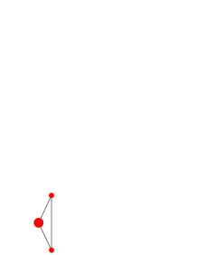
Figure 6: A swimming triangle on the sphere and the pseudosphere. The oars are long and their total weight equals the weight of the payload.

B.2.2 Swimming triangles

Consider an isosceles triangle made of two identical point masses $m$ at the base so that the total mass of the swimmer is $M$. For a the triangle of height $h$ and base $b$ (whose center of mass is at the origin) one has

$$\frac{8}{M}\,\left(\sum m_{n}\,x_{n}\,y^{2}_{n}\right)=4\frac{m(M-2m)}{M^{2}}\,h\,b^{2}\leq\frac{1}{2}\,hb^{2}$$ (B.10)

and the optimizer is when $4m=M$. The optimal weight distribution has oars whose weight balances the weight of the payload. The dependence on $b$ may be interpreted as the statement that a good swimmer needs long oars. If the swimming stroke is a rectangle in the $(b,h)$ plane with sides $(\delta b,\delta h)$ then $dA=(\delta b/b)(\delta h/h)$ and the swimming distance $\delta x$ is at most $\mbox{$1\over 2$}b\,\delta b\,\delta h$.

References

- [1] Arthur Besse, Einstein manifolds, Springer
- [2] S.K. Blau, Phys. Today 56 21 (2003); C. Seifer, Science, 299 1295 (2003)
-
[3]
A video of a falling cat can be found in
http://www.photomuseum.org.uk/insight/info/dropcat.mov - [4] W. G. Dixon, Dynamics of extended bodies in general relativity. I. Momentum and angular momentum, Proc. Roy. Soc. London, A, (1970); A Covariant Multipole Formalism for Extended Test Bodies in General Relativity, Nuovo Cimento, (1964);Extended bodies in general relativity: Their description and motion
- [5] E. Gueron, C. A. S. Maia, and G. E. A. Matasas arXiv:gr-qc/051005
- [6] H. Knörrer made a dramatized physics class on the falling cat problem http://www.math.ethz.ch/ knoerrer/knoerrer.html
- [7] L.D. Landau and E.M. Lifshitz, Classical Mechanics, Pergamon (1960).
- [8] R.G. Littlejohn and M. Reinsch, Gauge fields in the separation of rotations and internal motions in the n-body problem, Rev. Mod. Phys. 69, 213-276 (1997).
- [9] M. J. Longo, Am. J. Phys. 72, 1312 (2004)
- [10] J. Marsden, Motion control and geometry, Proceeding of a Symposium, National Academy of Science 2003; R. Montgomery, Fields Institute Comm. 1, 193 (1993); J. Avron, O. Gat, O. Kenneth and U. Sivan, Optimal rotations of deformable bodies and orbits in magnetic fields, Phys. Rev. Lett. 92, 040201-1 (2004).
- [11] Rudolph Erich Raspe, The Surprising Adventures of Baron Munchausen
- [12] A. Shapere and F. Wilczek, J. Fluid Mech., 198, 557-585 (1989)
- [13] J. Wisdon, Swimming in Spacetime: Motion by Cyclic Changes in Body Shape, Science 299, 1865-1869, (2003)
- [14] R. M. Wald, General relativity, Appendix C.3, The University of Chicago Press, (1984)