CERN-TH/96-317

SHEP 96-31

Gauge-Invariant Renormalization Group

at Finite Temperature

M. D’Attanasio

Department of Physics, University of Southampton,

Southampton SO17 1BJ, United Kingdom

M. Pietroni

Theory Division, CERN

CH-1211 Geneva 23, Switzerland

We propose a gauge-invariant version of Wilson Renormalization Group for thermal field theories in real time. The application to the computation of the thermal masses of the gauge bosons in an SU($N$) Yang-Mills theory is discussed.

CERN-TH/96-317
November 1996

1 Introduction

It is commonly believed that QCD at high temperature $T\gg\Lambda_{\rm QCD}$ is in a deconfined phase, that is the system is composed by a gas of quarks and gluons interacting with a coupling $\alpha_{\rm QCD}(T)\ll 1$. Therefore perturbation theory is reliable at energy scales of order $T$. This picture runs into problems when one probes the softer scale $gT$, where contributions of the same order are generated at every order in perturbation theory [1]. At high temperature the relevant $gT$ contributions are obtained by resumming the one-loop Feynman diagrams (Hard Thermal Loop resummation [2]).

However, in non-Abelian gauge theories there is another major obstacle in performing perturbative computations. Since the static magnetic fields are not screened at HTL level, one finds wild infrared divergences at order $g^{2}T$, scale in which one expects such a magnetic mass to be dynamically generated by the interacting theory. Therefore there is a need for new resummation methods.

In ref. [3] we proposed a possible approach. The basic idea is to consider a “cold” $T=0$ quantum system and add thermal fluctuations at lower and lower frequency scales, until the non-perturbative scale $g^{2}T$ is reached. In this way the system is thermalized at larger and larger distances until the scale $g^{2}T$ is reached “smoothly”. This corresponds to performing a coarse-graining à la Wilson [4] for the thermal fluctuations. We will call such a method Thermal Renormalization Group (TRG).

This approach is inspired by continuum Wilson or “Exact” Renormalization Group (ERG) [5]–[9], in which one starts with the microscopic ultraviolet action and adds quantum modes with frequency larger than a coarse-graining scale $\Lambda$. By continuously varying $\Lambda$ one gets the ERG flow equations in the form of partial differential equations in $\Lambda$, which can be integrated to obtain the full quantum theory at $\Lambda=0$. The main difficulty associated to the application of ERG to $T=0$ gauge theories is that it is not possible to introduce the infra-red cut-off $\Lambda$ in a gauge-invariant way. Therefore the Slavnov-Taylor identities of the theory are violated and one can only hope to recover them once the cut-off is removed [6, 10]–[13].

One encounters similar difficulties when the ERG is applied to thermal field theories. If one tries to perform a coarse-graining of both quantum and thermal fluctuations, the ST identities are necessarily violated by the coarse-graining scale $\Lambda$ and it is much more difficult to extract gauge-invariant quantities (see for instance [14]).

However, as explained above, the problem is simpler if one is interested in resumming à la Wilson the thermal modes only, namely in TRG. One assumes that the $T=0$ renormalized quantum field theory is known (from experiments, perturbation theory, lattice or other approximation methods) and adds thermal fluctuations for frequencies $|\vec{k}|>\Lambda$. In this way one interpolates between the renormalized theory at $T=0$ ($\Lambda=\infty$, no thermal modes have been integrated out) and the theory in thermal equilibrium at temperature $T$ ($\Lambda=0$, all the thermal modes have been integrated out).

For a finite value of the cut-off $\Lambda$ one is describing a physical, i.e. renormalized, system out of thermal equilibrium, with a $\Lambda$-dependent density matrix $\rho(\Lambda)$. From a physical point of view, the better status of gauge symmetry in this approach can be easily understood. Indeed, the expectation values and the Green functions in an out-of-equilibrium system differ from those at $T=0$ (and from those in thermal equilibrium) because of the different weights of the physical states in the thermal average. But, as long as no unphysical states are introduced, the BRS variation and the thermal averaging are commuting operations and the Slavnov-Taylor identities are completely analogous to the ones at $T=0$, provided the vacuum expectation values are interpreted as thermal averages with respect to the density matrix $\rho(\Lambda)$ [15].

From a technical point of view, varying the density matrix corresponds to changing the temporal boundary condition that has to be given in order to invert the quadratic part in the Lagrangian and define the free propagator. The Lagrangian itself is not modified and retains all its symmetries. This is to be contrasted with the usual formulation of the Wilson RG in which the introduction of the cut-off breaks the BRS invariance of the Lagrangian explicitly [6, 10]–[13, 14].

In order to implement this modification of the temporal boundary conditions we need a real-time formalism suited to describe a system with an arbitrary initial density matrix. Therefore we find it appropriate to use the Closed Time Path (CTP) method [15]–[18], which is a general formalism to deal with out of equilibrium problems. The CTP technique is a generalization of the Real Time (RT) [19] formulation of equilibrium thermal field theories and involves a doubling of the degrees of freedom.

In CTP the information about the initial state is encoded in source terms concentrated at $t=t_{0}\rightarrow-\infty$. By invoking an adiabatic switching-off for the couplings, such information is contained as boundary conditions in the free propagators. By giving equilibrium boundary conditions, one recovers the path-integral representation for the generating functional of the usual Real Time equilibrium thermal field theory given, for instance, in ref. [24]. We modify the boundary conditions by introducing a momentum-dependent temperature $\beta(|\vec{k}|)$ such that the path-integral representation for our coarse-grained generating functionals can be obtained by substituting, in the equilibrium path-integral, the Bose distribution for a cut-off one

$$N_{b}(|k_{0}|)\to N_{b}(|k_{0}|,\Lambda)=\theta(|\vec{k}|-\Lambda)\,N_{b}(|k_{0}|)\,.$$ (1)

By varying with respect to $\Lambda$ we will obtain the TRG flow equations for the generating functional and for all the Green functions of the theory.

Integrating the flow equations from $\Lambda=\infty$ to $\Lambda=0$, the resummed Green functions to all orders in thermal perturbation theory are obtained.

Another advantage of using the TRG in studies at high temperature is that the boundary condition for the flow equations at $\Lambda\gg T$ is just the full quantum theory at $T=0$, which is directly related to the physical parameters. The presence of the infra-red cut-off allows a reliable computation of the initial conditions in the framework of zero temperature perturbation theory.

A good and clear control over the initial conditions is indeed a necessary requirement when one is interested in small thermal effects such as the generation of a magnetic mass for the gluon, which we expect to be $O(g^{2}T)$. On the other hand, using as initial condition the bare theory at some ultraviolet cut-off, as one is forced to do in the ERG, the connection between the physical parameters and the initial ones is obtained only after the pure quantum corrections have been included via some approximation of the flow equations at $T=0$.

There is another advantage in using the real time TRG instead of ERG at finite temperature in the imaginary time. In a non-interacting thermal gauge field theory it is not necessary to give thermal fluctuations to the unphysical degrees of freedom, such as ghosts and longitudinal gluons (only physical transverse particles are in contact with the thermal bath and get heated). Therefore the Feynman rules to construct perturbation theory can be simplified in such a way that only the propagator of transverse gluons receives thermal boundary conditions. This is true both in physical gauges (such as axial [20]–[22]) and covariant gauges [23]. In this way only the transverse modes of the gluons have to be coarse-grained and one gets simplified TRG flow equations. This approach is denoted as TRG in physical phase space and is very useful if one wants to exploit TRG as a real computational tool.

The paper is organized as follows. In Sect. 2 the CTP formulation for an SU($N$) gauge theory is briefly discussed. In Sect. 3 the TRG flow equations are derived and the kernel is discussed. In Sect. 4 we derive the ST identities and show that they are the same as those for the theory without the cut-off on the thermal sector. In Sect. 5 the computation of the electric and magnetic screening masses at order $g^{2}T$ in the TRG formalism is discussed. The appendices contain some technical details.

2 Closed Time Path for pure gauge SU($N$) theory

In this paper we will specialize to the case of an SU($N$) Yang-Mills theory. The inclusion of fermions and other matter fields poses no conceptual difficulties.

The action is

$$S=\int{d}^{4}x\,\biggr{\{}-\frac{1}{4}\left(F_{\mu\nu}\cdot F_{\mu\nu}\right)-\frac{1}{2\alpha}{\cal F}^{2}-\bar{c}\cdot{\cal M}\cdot c\biggl{\}}\,,$$ (2)

where

$$F^{a}_{\mu\nu}(x)=\partial_{\mu}A^{a}_{\nu}-\partial_{\nu}A^{a}_{\mu}+g\left(A_{\mu}\wedge A_{\nu}\right)^{a}\,,\;\;\;\;\;\;\left(A_{\mu}\wedge A_{\nu}\right)^{a}=\epsilon^{abc}A^{b}_{\mu}A^{c}_{\nu}\,,$$

$$F_{\mu\nu}\cdot F_{\mu\nu}=F_{\mu\nu}^{a}F_{\mu\nu}^{a}\,,\;\;\;\;\;\;D_{\mu}c=\partial_{\mu}c+gA_{\mu}\wedge c\,;$$

${\cal F}[A_{\mu}]$ is the gauge-fixing term and ${\cal M}$ the Fadeev-Popov operator. The metric tensor $(1,-1,-1,-1)$ and the colour indices will be understood in the following.

The action (2) is invariant under the BRS transformations

$$\delta A_{\mu}=\eta D_{\mu}c\,,\;\;\;\;\;\;\;\delta c=-\eta\frac{g}{2}c\wedge c\,,\;\;\;\;\;\;\;\delta\bar{c}=-\frac{1}{\alpha}\eta{\cal F}[A_{\mu}]\,,$$ (3)

with $\eta$ a Grassmann parameter. In many formulae the fields and corresponding sources will be denoted by

$$\Phi=(A,\,c,\,\bar{c})\,,\quad\quad J=(j,\,\bar{\chi},\,-\chi)\,.$$ (4)

As we stated in the introduction, our formulation of the TRG is based on a deformation of the density matrix of the system implemented by introducing an infra-red scale $\Lambda$ such that for $\Lambda\rightarrow\infty$ the system is at zero temperature and at $\Lambda\rightarrow 0$ it is in thermal equilibrium at a temperature $T$. For intermediate values of $\Lambda$, only the high-momentum modes with $|\vec{k}|>\Lambda$ are in thermal equilibrium, whereas the low-momentum ones are frozen at $T=0$.

In order to describe this system for a generic value of $\Lambda$, we shall use the CTP formalism introduced in [16], which is designed for a system prepared at some initial time $t_{0}$ with a generic density matrix $\rho$. In our applications the limit $t_{0}\rightarrow-\infty$ is always understood.

The partition function can be represented as a path integral in which the time argument of the fields takes values on a path going from an initial time $t_{0}$ to $t=+\infty$ along the real time axis, and then back to $t_{0}-i\varepsilon$ infinitesimally below it. Indicating with $\Phi^{1}$ and $\Phi^{2}$ the fields with time arguments on the upper and lower pieces of the time path, respectively, the partition function is given by (for the proof of this and more details on the CTP method the reader is referred to [17]):

$$Z[J^{1},J^{2},\rho]=\int[{d}\Phi]\langle\Phi^{1},t=t_{0}|\rho|\Phi^{2},t=t_{0}\rangle\exp i\left\{\mbox{\small$\frac{1}{2}$}\mathop{\mathrm{Tr}}\Phi\cdot D_{0}^{-1}\cdot\Phi+S_{\rm int}[\Phi]+\mathop{\mathrm{Tr}}J\cdot\Phi\right\}\,,$$ (5)

where

$$[{d}\Phi]=[{d}\Phi^{1}][{d}\Phi^{2}]\,,$$

$$\mbox{\small$\frac{1}{2}$}\mathop{\mathrm{Tr}}\,\Phi\cdot D_{0}^{-1}\cdot\Phi=\sum_{i,j=1,2}\int\frac{{d}^{4}p}{(2\pi)^{4}}\left\{\mbox{\small$\frac{1}{2}$}A_{\mu}^{i}(p)\,[{\bf G_{0}}^{-1}_{\mu\nu}(p)]^{ij}\,A_{\nu}^{j}(-p)+\bar{c}^{i}(p)\,[{\bf S_{0}}^{-1}(p)]^{ij}\,c^{j}(-p)\right\}\,,$$

$$\mathop{\mathrm{Tr}}\,J\cdot\Phi=\int\frac{{d}^{4}p}{(2\pi)^{4}}\left\{j_{\mu}^{1}(-p)A_{\mu}^{1}(p)+\bar{\chi}^{1}(-p)c^{1}(p)+\bar{c}^{1}(-p)\chi^{1}(p)\>\>-\>\>1\to 2\right\}$$

and $S_{\rm int}[\Phi]$ is the bare interaction action

$$S_{\rm int}[\Phi]=S_{\rm int}[\Phi^{1}]-S_{\rm int}[\Phi^{2}].$$ (6)

${\bf G_{0}}_{\mu\nu}$ and ${\bf S_{0}}$ are the gauge and ghost free propagator, respectively (the $2\times 2$ CTP matrices are indicated in bold face).

In order to define the BRS transformation at the quantum level, source terms for the composite operators appearing in (3), that is

$$w_{\mu}^{1}(D_{\mu}c)^{1}-\frac{g}{2}v^{1}c^{1}\wedge c^{1}\>\>-\>\>1\to 2\,,$$ (7)

have to be added to (5). In the following the dependence on the sources $w_{\mu}$ and $v$ will be understood.

In order to construct a perturbation theory for the path integral (5), one assumes that initial correlations at $t=t_{0}$ have a small effect on the system at much larger times. This hypothesis is equivalent to adiabatically switching off the interactions for $t\rightarrow t_{0}$ [24]. In this way the initial states $|\Phi^{i},t=t_{0}\rangle$ ($i=1,\,2$) are the physical states of the non-interacting theory (this requires special care in the case of a gauge theory, where the Hilbert space is larger than the physical space—we will come back to this issue in the following). Moreover the initial density matrix describes a free system and can then be taken diagonal, that is

$$\rho\sim\exp\left\{-\int{d}^{3}k\,\beta(\vec{k})\sum_{{\rm phys.}\>{\rm states}}a^{\dagger}_{\vec{k}}a_{\vec{k}}\right\}\,,$$ (8)

where as usual $a_{\vec{k}}$ is the annihilation operators for the free initial state $|\Phi(\vec{k}),t=t_{0}\rangle$ of momentum $\vec{k}$ (for simplicity we choose the same “temperature” $\beta(\vec{k})$ for all modes). The density matrix (8) is a generalization of the equilibrium density matrix, which is obtained for $\beta(\vec{k})=\beta\omega_{|\vec{k}|}$. The matrix elements of (8) at $t=t_{0}$ can be represented in the following way [17]:

$$\langle\Phi^{1},t=t_{0}|\rho|\Phi^{2},t=t_{0}\rangle=\exp\left\{i\mbox{\small$\frac{1}{2}$}\int K^{ij}\Phi^{i}\Phi^{j}\right\}\,.$$ (9)

Therefore the statistical information on the initial state is all contained in the non-local boundary source $K^{ij}(t_{0},\vec{x};t_{0},\vec{x}^{\prime})$, which is concentrated around $t=t_{0}$. $K^{ij}$ is just the boundary condition in time needed in order to invert the d’Alembertian operator and to define the free propagator. Notice that with a diagonal density matrix, as in (8), the boundary sources $K^{ij}$ can be computed exactly (see [17] and below).

Our goal is a path integral representation of a system with modes thermalized for scales $|\vec{k}|>\Lambda$. This can be obtained, according to (1), by choosing $\beta(\vec{k})=\beta_{\Lambda}(\vec{k})$, where

$$\beta_{\Lambda}(\vec{k})=\left\{\begin{array}[]{cc}\beta\omega_{|\vec{k}|}&{\rm for}\;\;|\vec{k}|>\Lambda\\ &\\ +\infty&{\rm for}\;\;|\vec{k}|<\Lambda\end{array}\right.\,.$$ (10)

In this way the boundary source $K^{ij}$ becomes $\Lambda$-dependent and the partition function of such a system can be written as

$$Z_{\Lambda}[J^{1},J^{2},\rho]=\int[{d}\Phi]\exp i\left\{\mbox{\small$\frac{1}{2}$}\mathop{\mathrm{Tr}}\Phi\cdot D_{0,\Lambda}^{-1}\cdot\Phi+S_{\rm int}[\Phi]+\mathop{\mathrm{Tr}}J\cdot\Phi\right\}\,,$$ (11)

where the appropriate source term $K_{\Lambda}$ has been absorbed in

$$D_{0,\Lambda}^{-1}\equiv D_{0}^{-1}+K_{\Lambda}\,.$$ (12)

In general, the free propagator (12) can be computed by performing the same manipulations as are done in the well-known equilibrium case $\beta(\vec{k})=$ constant [17]. Therefore in a scalar theory [3] $D_{\Lambda}$ is obtained from the one in the real time equilibrium formalism of Niemi and Semenoff [19], with the obvious substitution $\beta\to\beta_{\Lambda}(\vec{k})$. This is equivalent to replacing the Bose-Einstein distribution function with the cut-off one as in (1).

When dealing with a gauge model, there is a further complication, namely, after gauge fixing, the Hilbert space and the set of physical states no longer coincide. As a consequence, the partition function cannot be generally defined as the trace over the whole Hilbert space of the density matrix $\rho$, but is instead given by

$$Z(\beta)=\mathop{\mathrm{Tr}}\left[{\rm P}\rho\right]\;,$$ (13)

where P is the projector onto the physical subspace.

We now consider separately the case of covariant and axial gauges.

2.1 Covariant gauges

In a covariant gauge, Fadeev-Popov (FP) ghosts and unphysical degrees of freedom populate the Hilbert space, and the projector P is non-trivial. This problem is of course closely related to the question of which temporal boundary conditions should be given to the FP ghosts and to the unphysical degrees of freedom of the gauge bosons, which could never come into equilibrium with the thermal bath.

In equilibrium thermal field theory there are mainly two approaches to handle this problem. The standard one (which we call the Bernard-Hata-Kugo approach) consists in giving periodic boundary conditions to the unphysical degrees of freedom [25, 26]. The other one (which we call the Landshoff-Rebhan approach) consists in giving thermal boundary conditions only to the physical (transverse) degrees of freedom [23]. We now describe how to generalize them to our TRG case.

(i) Bernard-Hata-Kugo approach. The basic observation behind this approach is that the partition function can be rewritten as

$$Z(\beta)=\mathop{\mathrm{Tr}}\left[e^{-\pi Q_{c}}\rho\right]\;,$$ (14)

where $Q_{c}$ is the FP ghost charge. Moreover, the thermal average of any gauge-invariant operator ${\cal O}$,

$$\langle{\cal O}\rangle\equiv\mathop{\mathrm{Tr}}\left[{\rm P}\rho\,{\cal O}\right]/\mathop{\mathrm{Tr}}\left[{\rm P}\rho\right]$$ (15)

is equal to

$$\langle{\cal O}\rangle=\mathop{\mathrm{Tr}}\left[e^{-\pi Q_{c}}\rho\,{\cal O}\right]/\mathop{\mathrm{Tr}}\left[e^{-\pi Q_{c}}\rho\right]\>\>\>\>\>\>\>\qquad{\rm if}\>\>\>\>\>\>[{\cal O},Q_{\rm BRS}]=0\;,$$ (16)

where $Q_{\rm BRS}$ is the BRS charge.

Since any physical observable must be BRS-invariant, Hata and Kugo proposed to modify the definition of a thermal average from eq. (15) to (16). This gives of course Green functions different from those obtained by using (15), but the result for physical quantities is unchanged. With this definition one can now derive path integral representations for the partition function and the Green functions by replacing $\rho$ with $\rho\exp(-\pi Q_{c})$ and enlarging the set of states $|\Phi^{i},t_{0}\rangle$ in (5) to the full Hilbert space. Strictly speaking, Hata and Kugo considered the case of an equilibrium density matrix $\rho$. However, as is shown in appendix A, it is straightforward to generalize their proof to the case in which $\rho$ has the form

$$\rho\sim\exp\left\{-\int{d}^{3}k\,\beta(\vec{k})\left[\sum_{\lambda=0}^{3}a^{(\lambda){\dagger}}_{\vec{k}}a^{(\lambda)}_{\vec{k}}+\mbox{\small$\frac{1}{2}$}\bar{c}^{{\dagger}}_{\vec{k}}c_{\vec{k}}-\mbox{\small$\frac{1}{2}$}c^{{\dagger}}_{\vec{k}}\bar{c}_{\vec{k}}\right]\right\}\,,$$ (17)

where $a^{(\lambda)}_{\vec{k}}$, $c_{\vec{k}}$ and $\bar{c}_{\vec{k}}$ are the annihilation operators for the free state of momentum $\vec{k}$ for gauge bosons with polarization index $\lambda$, ghost and antighost, respectively. In the special case of thermal equilibrium, $\beta(\vec{k})=\beta\omega_{|\vec{k}|}$, this corresponds to assigning periodic boundary conditions to all the bosonic degrees of freedom and also to the FP ghosts. This is the approach that has been traditionally followed in the applications of perturbative thermal field theory to gauge theories.

As explained in the previous section the TRG formulation is obtained by choosing the “temperature” $\beta(\vec{k})$ as in (10). The computation of the boundary source $K_{\Lambda}$ is completely analogous to the equilibrium case. The free TRG gauge propagator is then the usual real time equilibrium gauge propagator [24], with the Bose distribution replaced by the cut-off one in eq. (1), that is

$${\mathbf{G}_{0}}_{\Lambda,\mu\nu}(k)=-\left(A_{\mu\nu}+B_{\mu\nu}+\alpha D_{\mu\nu}\right)\;\biggl{\{}{\mathbf{Q}}[\Delta_{0}(k)]+[\Delta_{0}(k)-\Delta_{0}^{*}(k)]\,N_{b}(|k_{0}|,\Lambda)\;{\mathbf{B}}\biggr{\}}\,,$$ (18)

where we introduced the notations

$${\mathbf{Q}}[f(k)]=\left(\begin{array}[]{cc}f(k)&(f(k)-f^{*}(k))\theta(-k_{0})\\ &\\ (f(k)-f^{*}(k))\theta(k_{0})&-f^{*}(k)\end{array}\right)$$ (19)

$${\mathbf{B}}=\left(\begin{array}[]{cc}1&1\\ &\\ 1&1\end{array}\right)\,,$$ (20)

and the free Feynman propagator

$$\Delta_{0}=\frac{1}{k^{2}+i\varepsilon}\,.$$

The usual basis of tensors

$$A_{\mu\nu}=g_{\mu\nu}-\frac{1}{(ku)^{2}-k^{2}}[(ku)(u_{\mu}k_{\nu}+u_{\nu}k_{\mu})-k_{\mu}k_{\nu}-k^{2}u_{\mu}u_{\nu}]\,,$$

$$B_{\mu\nu}=\frac{-k^{2}}{(ku)^{2}-k^{2}}\left(u_{\mu}-\frac{(ku)k_{\mu}}{k^{2}}\right)\left(u_{\nu}-\frac{(ku)k_{\nu}}{k^{2}}\right)\,,$$

(21)

$$C_{\mu\nu}=\frac{1}{\sqrt{2[(ku)^{2}-k^{2}]}}\left[\left(u_{\mu}-\frac{(ku)k_{\mu}}{k^{2}}\right)k_{\nu}+\left(u_{\nu}-\frac{(ku)k_{\nu}}{k^{2}}\right)k_{\mu}\right]\,,$$

$$D_{\mu\nu}=\frac{k_{\mu}k_{\nu}}{k^{2}}$$

satisfy the multiplication properties

$$A\cdot B=A\cdot C=A\cdot D=0\;,\;\;\;\;\;A+B+D=1\;,$$

$$A\cdot A=A\;,\;\;\;B\cdot B=B\;,\;\;\;C\cdot C=\mbox{\small$\frac{1}{2}$}(B+D)\;,$$

$$\mathop{\mathrm{Tr}}C\cdot B=\mathop{\mathrm{Tr}}C\cdot D=0\;.$$ (22)

In the thermal reference frame we have $u_{\mu}=(1,0,0,0)$, and therefore the only non-vanishing components of $A$ are the spatial ones, giving the transverse tensor

$$A_{ij}=-\delta_{ij}+\frac{k_{i}k_{j}}{|{\vec{k}}|^{2}}\,,$$ (23)

In the $\varepsilon\rightarrow 0$ limit, we have

$$\Delta_{0}(k)-\Delta_{0}^{*}(k)\longrightarrow-2i\pi\delta(k^{2})\,,$$ (24)

that is, the thermal part of the tree-level propagator involves on-shell degrees of freedom only (only real particles belong to the thermal bath). The free TRG ghost propagator is the same as for a scalar massless particle (notice again the cut-off Bose distribution):

$${\mathbf{S}_{0}}_{\Lambda}(k)=-{\mathbf{Q}}[\Delta_{0}(k)]-[\Delta_{0}(k)-\Delta_{0}^{*}(k)]\,N_{b}(|k_{0}|,\Lambda)\;{\mathbf{B}}\,,$$ (25)

(ii) Landshoff-Rebhan approach. A second possible formulation of thermal gauge theories in covariant gauges is obtained by restricting the space of initial states $|\Phi^{i},t_{0}\rangle$ to the physical one, as required by the original definition of the partition function, eq. (13). One has to recall that the initial state is given by free particles. In the case of an SU($N$) gauge theory, this means that only the gauge boson states with spatially transverse polarization will contribute to the trace, and consequently only the transverse components of the gauge fields will couple to $K$-sources. This corresponds to choosing an initial density matrix $\rho$

$$\rho\sim\exp\left\{-\int{d}^{3}k\,\beta(\vec{k})\sum_{\lambda=1}^{2}a^{(\lambda){\dagger}}_{\vec{k}}a^{(\lambda)}_{\vec{k}}\right\}\,,$$ (26)

where the sum over $\lambda$ now runs over transverse polarizations only.

In the case of thermal equilibrium, this choice leads to the Landshoff-Rebhan formulation of Real Time thermal field theory [23].

The TRG formulation is again obtained by using the cut-off Bose distribution. The TRG free propagator is then

$${\mathbf{G}_{0}}_{\Lambda,\mu\nu}(k)=-A_{\mu\nu}\;{\mathbf{P}}_{\Lambda}[\Delta_{0}(k)]-\left(B_{\mu\nu}+\alpha D_{\mu\nu}\right)\;{\mathbf{Q}}[\Delta_{0}(k)]\,,$$ (27)

where we introduced the compact notation

$${\mathbf{P}}_{\Lambda}[\Delta_{0}]={\mathbf{Q}}[\Delta_{0}(k)]+[\Delta_{0}(k)-\Delta_{0}^{*}(k)]N_{b}(|k_{0}|,\Lambda){\mathbf{B}}\;.$$

The free ghost propagator is simply the $T=0$ one:

$${\mathbf{S}_{0}}(k)=-{\mathbf{Q}}[\Delta_{0}(k)]\,.$$ (28)

Compared to the standard TRG propagators in (18) and (25), we see that only the transverse component of the free gauge propagator proportional to $A_{\mu\nu}$ gets a thermal structure, which incidentally is gauge-parameter-independent.

In the practical applications of the TRG in covariant gauges, the formulation à la Landshoff-Rebhan turns out to be more convenient, due to the absence of thermal ghost loops.

2.2 Temporal Axial Gauge

In physical gauges, such as axial or Coulomb ones, the Hilbert space contains no unphysical states, and then P=1. In particular the ghosts decouple.

The derivation of a path integral representation in these gauges then goes on analogously to what is done for the Landshoff-Rebhan case in covariant gauges, with only the physical transverse gluon modes included in the density matrix (8).

Here we are mainly interested in the Temporal Axial Gauge (TAG), which is obtained by taking ${\cal F}^{a}=u_{\mu}A^{a}_{\mu}$ in (2), with $u_{\mu}=(1,0,0,0)$, and letting $\alpha\rightarrow\infty$.

The TAG is not a “good” gauge, in the sense that the gauge is not completely fixed by the choice $A_{0}^{a}=0$. This gauge freedom manifests itself in the spurious $1/k_{0}$ poles in the longitudinal part of the free propagator. In the framework of perturbation theory, different prescriptions have been proposed to circumvent these singularities. In particular in the real time formalism at $T\neq 0$ the issue has been studied by James in ref. [20]. As we will discuss in subsect. 4.2, when computing the gauge-independent pole masses using the TRG, all the terms containing these spurious poles cancel. So in our applications it is not necessary to fix a particular prescription.

The free TAG TRG propagator in covariant form is given by [20]

$${\mathbf{G}_{0}}_{\Lambda,\mu\nu}=-A_{\mu\nu}\;{\mathbf{P}}_{\Lambda}[\Delta_{0}(k)]-{\bf{Q}}^{\prime}\left[H_{\mu\nu}\Delta_{0}(k)\right]\;,$$ (29)

where

$$H_{\mu\nu}\equiv B_{\mu\nu}-\frac{\sqrt{2}|\vec{k}|}{k_{0}^{\prime}}C_{\mu\nu}-\frac{|\vec{k}|^{2}}{k_{0}^{\prime 2}}D_{\mu\nu}\;,$$ (30)

and ${\mathbf{Q}}^{\prime}$ and $k_{0}^{\prime}$ has been chosen for definiteness according to James’s prescription, i.e.

$${\mathbf{Q}^{\prime}}[f(k)]=\left(\begin{array}[]{cc}f(k)&(f(k)-f^{*}(k))\theta(-k_{3})\\ &\\ (f(k)-f^{*}(k))\theta(k_{3})&-f^{*}(k)\end{array}\right)$$ (31)

and $k_{0}^{\prime}=k_{0}+i\varepsilon/k_{3}$.

3 TRG evolution equations

By taking the derivative with respect to $\Lambda$ of (11) we obtain the evolution equation for $Z_{\Lambda}[J]$,

$$\Lambda\frac{\partial\>\>}{\partial\Lambda}Z_{\Lambda}[J] = -i(2\pi)^{8}{\rm Tr}\left\{\mbox{\small$\frac{1}{2}$}\Lambda\frac{\partial\>\>}{\partial\Lambda}D^{-1}_{0\Lambda}\cdot\frac{\delta^{2}Z_{\Lambda}[J]}{\delta J\delta J}\right\}$$

$$= -i(2\pi)^{8}{\rm Tr}\left\{\mbox{\small$\frac{1}{2}$}\frac{\delta\>\>}{\delta j_{\mu}}\cdot\Lambda\frac{\partial\>\>}{\partial\Lambda}{\mathbf{G_{0}}}_{\Lambda,\mu\nu}^{-1}\cdot\frac{\delta\>\>}{\delta j_{\nu}}Z_{\Lambda}[J]\right\}\,.$$

In deriving the second equation the ghost propagator has been assumed to be $\Lambda$-independent, as in TRG in physical phase space. Therefore all the discussion below holds only in such a case. However, the flow equation in the Bernard-Hata-Kugo approach can be obtained straightforwardly by including also the $\Lambda$-dependence of the free propagator of the ghost.

Choosing as initial conditions for $Z_{\Lambda}[J]$ at $\Lambda\gg T$ the full renormalized theory at zero temperature, the above evolution equation describes the effect of the inclusion of the thermal fluctuations at the momentum scale $|{\vec{k}}|=\Lambda$. At a certain scale $\Lambda$ we are describing a system in which only the high-frequency modes $|{\vec{k}}|>\Lambda$ are in thermal equilibrium. The low-frequency modes do not feel the thermal bath and behave like zero-temperature, quantum modes.

We define as usual the cut-off effective action as the Legendre transform of the generating functional of the connected Green functions $W_{\Lambda}[J]=-i\log Z_{\Lambda}[J]$:

$$\mbox{\small$\frac{1}{2}$}\mathop{\mathrm{Tr}}\,\Phi\cdot({{D_{0}}}_{\Lambda}^{-1}-{{D_{0}}}^{-1})\cdot\Phi+\Gamma_{\Lambda}[\Phi]=W_{\Lambda}[J]-\mathop{\mathrm{Tr}}\,J\cdot\Phi\,,\quad\quad\Phi(p)=(2\pi)^{4}\frac{\delta W_{\Lambda}[J]}{\delta J(-p)}\,,$$ (33)

where we have isolated the effect of the cut-off on the free part of the effective action and used for the classical fields the same notation as for the quantum fields.

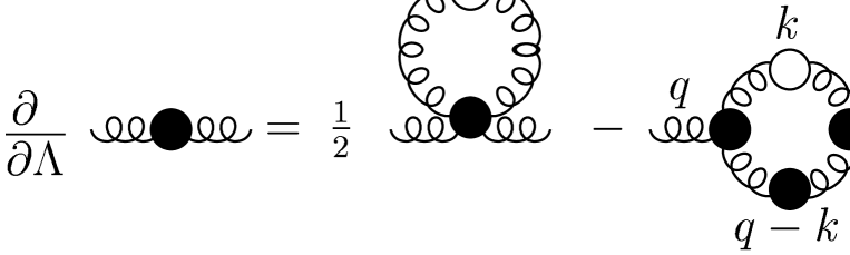
Figure 1: Flow equation for the self-energy in the physical space. The black circles are the full 1-particle-irreducible vertices, while the white circles represent the TRG kernel, given by eq. (40).

The evolution equation for the cut-off effective action $\Gamma_{\Lambda}[\Phi]$ can be derived straightforwardly from eq. (3). This is done in appendix B. The flow equations for the proper vertices are obtained by derivation of the one for the effective action. As an illustration, the flow equation for the gauge boson self-energy is given in eq. (72) and depicted in Fig. 1. We see that the recipe to obtain the TRG flow equations is very simple: one takes the one-loop graphs, substitutes every vertex and propagator with the full ones, apart from a propagator that becomes the RG kernel:

$${\bf K}_{\Lambda,\mu\nu}=i{\mathbf{G}}_{\Lambda,\mu\rho}\cdot\Lambda\frac{\partial\>\>}{\partial\Lambda}{\mathbf{G}_{0}}_{\Lambda,\rho\tau}^{-1}\cdot{\mathbf{G}}_{\Lambda,\tau\nu}\,,$$ (34)

where the full propagator

$${\mathbf{G}}_{\Lambda,\tau\nu}=\left({\mathbf{G}_{0}}_{\Lambda,\tau\nu}^{-1}-{\mathbf{\Sigma}}_{\Lambda,\tau\nu}\right)^{-1}$$ (35)

appears. Since the only $\Lambda$-dependent part in ${\mathbf{G}}_{\Lambda,\rho\tau}$ is proportional to the tensor $A_{\mu\nu}$ defined in eq. (21), and using the fact that $A_{\mu\nu}$ is orthogonal to the remaining three tensors, the only component of the full propagator needed in order to compute the kernel is the one proportional to $A_{\mu\nu}$. It has the general form

$$A_{\mu\rho}{\mathbf{G}}_{\Lambda,\rho\nu}=-A_{\mu\nu}{\mathbf{P}}^{\prime}_{\Lambda}[\Delta_{\rm T}(k)]\;,$$ (36)

where we defined

$${\mathbf{P}}^{\prime}_{\Lambda}[f(k)]={\mathbf{Q}}[f(k)]+[f(k)-f^{*}(k)]\,N_{b}^{\prime}(|k_{0}|,\Lambda)\;{\mathbf{B}}\,,$$ (37)

and we introduced the “longitudinal” and “transverse” Feynman propagators and self-energies

$$\Delta_{\rm L,T}(k)=\frac{1}{k^{2}-\Pi_{\rm L,T}(k)+i\varepsilon}\,.$$ (38)

The primes keep track of the fact that, in a generic gauge, the thermal structures appearing in the full propagator may correspond to an effective momentum-dependent temperature different from the physical one (see ref. [29]). However, multiplying the three matrices appearing in (34), it is easy to see that all the terms proportional to $N_{b}^{\prime}(|k_{0}|,\Lambda)$ drop, and the only temperature appearing in the kernel is the physical one, coming from the free propagator. The kernel can then be written as

$${\bf K}_{\Lambda,\mu\nu}(k)=-iA_{\mu\nu}(\Delta_{0}-\Delta_{0}^{*})\frac{\Delta_{\rm T}\Delta_{\rm T}^{*}}{\Delta_{0}\Delta_{0}^{*}}\>\Lambda\,\delta(|{\vec{k}}|-\Lambda)\,N_{b}(|k_{0}|)\;{\bf B}.$$ (39)

The above expression does not vanish in the $\varepsilon\rightarrow 0$ limit, and we obtain

$${\bf K}_{\Lambda,\mu\nu}(k)=-A_{\mu\nu}\,\rho_{{\rm T},\Lambda}(k)\epsilon(k_{0})\;\Lambda\,\delta(|{\vec{k}}|-\Lambda)\,N_{b}(|k_{0}|)\;{\bf B}\,,$$ (40)

where $\epsilon(k_{0})=\theta(k_{0})-\theta(-k_{0})$ and the transverse full spectral function,

$$i\rho_{{\rm T},\Lambda}(k)=\epsilon(k_{0})\,{\rm Disc}\,\Delta_{\rm T}(k),$$ (41)

appears. From (39) we note that the product of the kernel and the inverse of the full gluon propagator vanishes in the $\varepsilon\rightarrow 0$ limit. This fact will be used in the next section to derive ST identities in the present formalism.

We see that the kernel is exactly transverse and, in a covariant gauge, independent of the gauge-fixing parameter $\alpha$. The same form holds in the TAG. It is also completely identical (apart from the tensor $A$) to the kernel of a scalar particle, which was studied in detail in ref. [3].

The physical meaning of this kernel is straightforward. As the infrared cut-off $\Lambda$ is lowered, the dispersion relation satisfied by the new modes coming into thermal equilibrium is not given by $k^{2}=m^{2}$ as in the $T=0$ free theory, but is determined by the full spectral function. In the approximation in which one neglects the imaginary part of the full self-energy this simply amounts to substitute the $T=0$ mass with the thermal, $\Lambda$-dependent one.

In section 5 we will discuss the application of the formalism outlined in this paper to the computation of the electric and magnetic mass in a high-temperature SU($N$) plasma.

4 Slavnov-Taylor identities

In general, the implementation of the Wilson RG in the framework of Quantum Field Theory requires special care when gauge theories are considered. The obvious reason is that the introduction of a momentum cut-off on the quantum fluctuations immediately leads to a breaking of gauge invariance. The modified (inverse) propagator induces extra-terms into the ST identities, which recover their usual form only in the $\Lambda\rightarrow 0$ limit [10, 11]. To see this explicitely, we follow ref. [11] and perform a BRS-variation (3) of the fields in the path integral of eq. (11) in order to obtain the expression generating all the ST identities. For definitness, we discuss the case of general covariant gauges, but the discussion goes closely analogously for any class of gauges. The ST identities for the proper vertices are obtained by derivation of the expression

$$\int\frac{d^{4}p}{(2\pi)^{4}}\left\{\frac{\delta{\Gamma}_{\Lambda}}{\delta A_{\mu}^{i}(p)}\frac{\delta{\Gamma}_{\Lambda}}{\delta w_{\mu}^{i}(-p)}-\frac{\delta{\Gamma}_{\Lambda}}{\delta c^{i}(p)}\frac{\delta{\Gamma}_{\Lambda}}{\delta v^{i}(-p)}-\frac{i}{\alpha}p^{\mu}A_{\mu}^{i}(p)\frac{\delta{\Gamma}_{\Lambda}}{\delta\overline{c}^{i}(-p)}\right.$$

(42)

$$\left.-{\bf R}_{\mu\nu,\,ij}^{\Lambda}(p)\frac{\delta^{2}W_{\Lambda}}{\delta w_{\nu}^{i}(-p)\delta j_{\mu}^{j}(p)}-{\bf\tilde{R}}_{ij}^{\Lambda}(p)\frac{\delta^{2}W_{\Lambda}}{\delta v^{i}(-p)\delta\chi^{j}(p)}-\frac{i}{\alpha}p^{\mu}{\bf\tilde{R}}_{ij}^{\Lambda}(p)\frac{\delta^{2}W_{\Lambda}}{\delta j_{\mu}^{i}(-p)\delta\overline{\chi}^{j}(p)}\right\}=0,$$

where we have defined ${\bf R}_{\mu\nu}^{\Lambda}$ and ${\bf\tilde{R}}^{\Lambda}(p)$ as the differences between the inverses of the cut-off and uncut-off free propagator for the gluons and the ghosts, respectively,

$${\bf R}_{\mu\nu}^{\Lambda}(p)\equiv{\bf G}_{\Lambda,\mu\nu}^{-1}-{\bf G}_{\mu\nu}^{-1}\,,\;\;\;\;\;\;\;\;{\bf\tilde{R}}^{\Lambda}(p)\equiv{\bf S}_{\Lambda}^{-1}-{\bf S}^{-1},$$ (43)

where the color indices have been understood.

In the first line of eq. (42) we recognize the usual expression for the ST identities obeyed by the full theory without the IR cut-off. The second line represents the breaking of BRS-invariance induced by the modification of the propagator. It vanishes for $\Lambda=0$, as it should.

Now, the main point is that while in the applications of the RG discussed in refs. [10, 11, 14] the second line of eq. (42) gives non-zero contributions for $\Lambda\neq 0$, in the present approach it vanishes identically, and the cut-offed Green functions obey the same ST identities as the ones of the full theory, the first line of eq. (42). This can be understood by looking at the difference between the ${\bf R}$’s in the two approaches. In refs. [10, 11, 14] the RG flow describes the effect of integrating out quantum fluctuations (or quantum plus thermal fluctuations in the case of ref. [14], where the imaginary time formalism for thermal field theory has been considered). Therefore the cut-off is introduced by modifying the free propagator according to

$$G_{\mu\nu}(p)\rightarrow G_{\Lambda,\mu\nu}(p)=G_{\mu\nu}(p)\Theta(p,\Lambda),$$ (44)

then

$$R_{\mu\nu}(p)=G_{\mu\nu}^{-1}(p)(\Theta(p,\Lambda)^{-1}-1),$$ (45)

and analogously for the ghost propagator. As shown in ref. [11] these expressions, inserted in the analogous of eq. (42) for the four-dimensional theory at zero temperature, give non-vanishing contributions such as a $\Lambda$-dependent gluon mass.

On the other hand in the present approach we are modifying only the thermal part of the propagators (18), (25), or (27), by the substitution of eq. (1). Considering for definitness the Landshoff-Rebhan approach, we have,

$${\bf R}_{\mu\nu}^{\Lambda} = (N_{b}(|p_{0}|,\Lambda)-N_{b}(|p_{0}|))\rho_{{\rm T},\Lambda}(p)A_{\rho\sigma}\epsilon(p_{0})\,{\bf G}_{\Lambda,\mu\rho}^{-1}\cdot{\bf B}\cdot{\bf G}_{\Lambda,\sigma\nu}^{-1}$$

$$\equiv (N_{b}(|p_{0}|,\Lambda)-N_{b}(|p_{0}|))\,{\bf G}_{\Lambda,\mu\rho}^{-1}\cdot{\bf\tilde{k}}_{\Lambda,\rho\sigma}\cdot{\bf G}_{\Lambda,\sigma\nu}^{-1}\,,$$

where ${\bf\tilde{k}}_{\Lambda,\rho\sigma}$ is proportional to the kernel ${\bf K}_{\Lambda,\rho\sigma}$. From the discussion of the kernel in the previous paragraph we realize that the above expression vanishes in the $\varepsilon\rightarrow 0$ limit unless it is sandwiched between two full gluon propagators. This is not the case for eq. (42) since, defining the amputated field-dependent functional ${\bf\tilde{W}}_{\nu\rho}^{ik}$ by

$$\frac{\delta^{2}W_{\Lambda}}{\delta w_{\nu}^{i}(-p)\delta j_{\mu}^{j}(p)}\equiv{\bf\tilde{W}}_{\nu\rho}^{ik}{\bf G}_{\Lambda,\rho\mu}^{kj}$$ (47)

we have

$${\bf R}_{\mu\nu,\,ij}^{\Lambda}(p)\frac{\delta^{2}W_{\Lambda}}{\delta w_{\nu}^{i}(-p)\delta j_{\mu}^{j}(p)}=(N_{b}(|p_{0}|,\Lambda)-N_{b}(|p_{0}|))\mathop{\mathrm{Tr}}\left[{\bf\tilde{k}}_{\Lambda,\rho,\sigma}\cdot{\bf G}_{\Lambda,\sigma\nu}^{-1}\cdot{\bf\tilde{W}}_{\nu\rho}\right]\;,$$ (48)

which vanishes in the $\varepsilon\rightarrow 0$ limit, since ${\bf\tilde{W}}_{\nu\rho}^{ik}(p)$ does not contain a ${\bf G}_{\Lambda,\rho\mu}^{ik}(p)$ factor. The same is true also in the Hata-Kugo approach, where the extra contributions to the second line of eq. (42) from longitudinal and gauge gluon degrees of freedom, and from the ghosts, all vanish by he same reason explained above.

The Green functions defined in our approach are then gauge-invariant, in the sense that they satisfy the usual ST identities, given by the first line of eq. (42) even in the presence of a cut-off $\Lambda\neq 0$.

The fact that our TRG formalism respects ST identities for every value of $\Lambda$ is a great advantage with respect to the other RG methods, both from the conceptual point of view, since a physical meaning can be given to the TRG quantities for every $\Lambda$ (one could also think of possible non-equilibrium applications), and from a computational point of view, since the ST identities make it possible to relate propagator and vertices in a non-perturbative way.

5 Application: the thermal masses

The basic tool to study the behaviour of a high-temperature plasma is linear response theory [30]. The perturbation of the thermal average of the vector potential induced by a weak source $\delta J^{a}_{\mu}$ is given by the well-known relation

$$\delta\overline{A}_{\mu}^{a}(x)=\int dy\;\Gamma_{\mu\nu}^{{\rm RET},ab}(x,y)\;\delta J^{b}_{\nu}(y)\,,$$ (49)

where we further assume that $D^{ba}_{\mu}\delta J^{a}_{\mu}=0$.

If we consider a source that is non-vanishing in only one direction in colour space, then the above relation is sufficient to determine the induced perturbations on the field strength operator and consequently on the gauge invariant chromo-electric and magnetic fields. The retarded propagator appearing in (49) is given by the difference between the 11 and 12 components of the full propagator (35), which is the object we will study. It is of course a gauge-dependent quantity, so the question arises of what physical information can be derived from it. As has been discussed in [31, 32] the poles of the $A_{\mu\nu}$- and $B_{\mu\nu}$- components of the full propagator are gauge-independent and describe the exponential screening of chromo-electric and magnetic fields, respectively.

In a generic gauge, the full propagator can be written as

$${\bf G}_{\Lambda,\mu\nu}={\mathbf{a}}A_{\mu\nu}+{\mathbf{b}}B_{\mu\nu}+{\mathbf{c}}C_{\mu\nu}+{\mathbf{d}}D_{\mu\nu}\,,$$ (50)

where ${\mathbf{a}}$, ${\mathbf{b}}$, ${\mathbf{c}}$ and ${\mathbf{d}}$ are gauge-dependent $2\times 2$ matrices, the thermal structure of which is also gauge-dependent [29].

Similarly, the self-energy can be generally decomposed as

$${\mathbf{\Sigma}}_{\Lambda,\mu\nu}(k)={\mathbf{G}_{0}}_{\Lambda,\mu\nu}^{-1}(k)-{\mathbf{G}}_{\Lambda,\mu\nu}^{-1}(k)\\ =A_{\mu\nu}{\mathbf{\Sigma}}_{\rm T}(k)+B_{\mu\nu}{\mathbf{\Sigma}}_{\rm L}(k)+C_{\mu\nu}{\mathbf{\Sigma}}_{c}(k)+D_{\mu\nu}{\mathbf{\Sigma}}_{d}(k)$$

(the $\Lambda$-dependence of the ${\mathbf{\Sigma}}$’s in the right-hand side has been omitted). In general a Slavnov-Taylor identity will provide a relation between the four matrices in (5), so that in a generic gauge the self-energy will be determined by three independent functions. Nevertheless, as discussed in [32] the pole structure of the temporal and longitudinal modes is identical. Thus there are only two independent physical modes; the spatially transverse and the longitudinal one.

The longitudinal and transverse self-energies are

$$\displaystyle{\mathbf{\Sigma}}_{\rm L}(k) \equiv B^{\mu\nu}{\mathbf{\Sigma}}_{\Lambda,\mu\nu}\,,$$

$$\displaystyle{\mathbf{\Sigma}}_{\rm T}(k) \equiv \mbox{\small$\frac{1}{2}$}A^{\mu\nu}{\mathbf{\Sigma}}_{\Lambda,\mu\nu}\,.$$

The real parts of the 11 components of ${\mathbf{\Sigma}}_{\rm L,T}$ coincide with the real parts of $\Pi_{\rm L,T}$ in eq. (38), which will denoted as $\Pi_{\rm L,T}^{R}$.

The two physical poles of the full propagator are then identified by the equations

$$k^{2}-\Pi_{\rm L}^{R}(k)=0\,,\qquad\qquad k^{2}-\Pi_{\rm T}^{R}(k)=0\,.$$ (52)

We are interested in the screening of static chromo-electric and magnetic fields. The relevant poles are then given by

$$m_{\rm L}^{2}(\Lambda) = \left.\Pi_{\rm L}^{R}(q)\right|_{q=q_{\rm L}}\,,$$

$$m_{\rm T}^{2}(\Lambda) = \left.\Pi_{\rm T}^{R}(q)\right|_{q=q_{\rm T}}\;,$$

where $q_{\rm L,T}=(q^{0}_{\rm L,T}=0,\,|\vec{q}_{\rm L,T}|^{2}=-m^{2}_{\rm L,T})$.

The masses defined in (LABEL:poles) are gauge-fixing-independent for any value of $\Lambda$, as can be shown by strictly following ref. [33], and considering variations in the gauge-fixing term which vanish for $t\rightarrow t_{0}$.

The evolution equations for $m_{\rm L}^{2}$ and $m_{\rm T}^{2}$ can then be written down as

$$\displaystyle\Lambda\frac{\partial\;\;\;}{\partial\Lambda}m_{\rm L}^{2} = \displaystyle\left.\frac{B^{\mu\nu}(q)F_{\mu\nu}(q)}{1+\frac{\partial\Pi_{\rm L}^{R}(q)}{\partial|\vec{q}|^{2}}}\right|_{q=q_{\rm L}}\,,$$

$$\displaystyle\Lambda\frac{\partial\;\;\;}{\partial\Lambda}m_{\rm T}^{2} = \displaystyle\left.\frac{\mbox{\small$\frac{1}{2}$}A^{\mu\nu}(q)F_{\mu\nu}(q)}{1+\frac{\partial\Pi_{\rm T}^{R}(q)}{\partial|\vec{q}|^{2}}}\right|_{q=q_{\rm T}}\;,$$

where (see eqs. (72) and (73))

$$F_{\mu\nu}(q)\equiv\Lambda\frac{\partial\;\;\;}{\partial\Lambda}{\mathbf{\Sigma}}_{\Lambda,\mu\nu}^{11}(q)=\mbox{\small$\frac{1}{2}$}\int\frac{d^{4}k}{(2\pi)^{4}}{\bf K}_{\Lambda,\rho\sigma}(k)\left[\Gamma^{11ij}_{\Lambda,\mu\nu\rho\sigma}(q,-q,k,-k)\right.$$

$$\qquad\qquad\left.-2\Gamma^{1ik}_{\Lambda,\mu\rho\lambda}(q,-k,k-q){\mathbf{G}}_{\Lambda,\lambda\tau}^{kl}(q-k)\Gamma^{1jl}_{\Lambda,\nu\sigma\tau}(-q,k,q-k)\right]\,.$$ (55)

To simplify the notation, the colour structure has been understood. In appendix C we verify explicitly that the running does not introduce any gauge dependence. Namely, we show that, when contracted with $B^{\mu\nu}(q)$ ($A^{\mu\nu}(q)$) and computed at $q=q_{\rm L}$ ($q_{\rm T}$), $F_{\mu\nu}(q)$ gives a gauge-independent result.

The system (LABEL:eveqm) has to be integrated from some initial $\Lambda_{0}\gg T$ down to $\Lambda=0$. At $\Lambda_{0}$ we have to insert the zero-temperature propagators and vertices in the right-hand-sides. These can be reliably computed using perturbation theory, since, due to the momentum delta-function in the kernel, eq. (40), the loop momentum is forced to be $|\vec{k}|=\Lambda_{0}\gg T\gg\Lambda_{\rm QCD}$ (the external momentum is $|\vec{q}|=m_{{\rm L},{\rm T}}(\Lambda_{0})\ll\Lambda_{0})$. In other words, the cut-off serves as IR regulator for the $T=0$ theory. As we decrease $\Lambda$ at $O(gT)$, an IR cut-off is generated in the longitudinal sector (the longitudinal, or Debye, mass), whereas in the transverse sector a magnetic mass of $O(g^{2}T)$ is believed to emerge non-perturbatively.

The resummation of the thermal fluctuations from $\Lambda\simeq T$ to $\Lambda\simeq gT$ corresponds to the resummation of Hard Thermal Loops performed by Braaten and Pisarski [2]. To go beyond that approximation, thermal fluctuations from $gT$ to $g^{2}T$ have to be integrated out. In a perturbative framework, like HTL resummation, the different scales are not clearly separated, and this is reflected, for instance, in the pathologies (gauge-dependence and logaritmic divergence) of the next-to-leading correction to $m_{\rm L}$ [31], which require the ad-hoc introduction of a magnetic mass term. In the next subsections we outline how this non-perturbative problem can be tackled in the TRG formalism, both in covariant and physical gauges.

5.1 Covariant gauges

The class of covariant gauges is specified by taking ${\cal F}^{a}=\partial^{\mu}A^{a}_{\mu}$ in eq. (2). The four matrices in (50) are then restricted by the ST identity:

$$k^{\mu}k^{\nu}G_{\Lambda,\mu\nu}=\alpha\;.$$ (56)

In Landau gauge ($\alpha=0$) we have the stronger relation $k^{\mu}G_{\Lambda,\mu\nu}=0$.

In order to obtain an explicit form for the full propagator to be inserted in the evolution equations for the thermal masses, we will neglect the imaginary part of the longitudinal gluon self-energy, which allows us to write the full propagator as

$${\mathbf{\Delta}}^{0}_{\Lambda,\mu\nu}(k)=A_{\mu\nu}\;{\mathbf{P}}_{\Lambda}[\Delta_{\rm T}]+B_{\mu\nu}\;{\mathbf{Q}}[\Delta_{\rm L}+\alpha c^{2}\Delta_{\rm L}^{2}\Delta_{0}]-\alpha C_{\mu\nu}\;{\mathbf{Q}}[c\Delta_{\rm L}\Delta_{0}]+\alpha D_{\mu\nu}\;{\mathbf{Q}}[\Delta_{0}]\,,$$ (57)

where $c(k)$ is a gauge-dependent function.

Due to the presence of the full three and four gluon vertices (see Fig. 1), and of the unknown function $c$, the system of coupled differential equations (LABEL:eveqm) is not closed. The knowledge of the $\Lambda$-dependent vertex functions would of course require the solution of their evolution equations which, in turn, involve higher vertex functions.

In order to get a manageable approximation, the system has to be truncated at some level, in practice by using a suitable approximation of the three and four gluon vertices. A crucial requirement on this approximation is that it respects the Slavnov-Taylor equation for the full vertices to the required level of accuracy. This is essential if one wants a gauge-independent determination of $m_{\rm L,T}^{2}$ which are gauge-independent quantities in the full theory. In practice we are interested in computing the squared masses at $O(g^{4}T^{2})$. Looking at eq. (LABEL:eveqm) we see that the most dangerous $\alpha$-dependent contribution comes from the $D_{\mu\nu}$-term in the propagator of eq. (57). If we just use the tree-level expression for the trilinear vertex, then, since

$$(k-p)_{\lambda}\Gamma_{\mu\rho\lambda}^{\rm tree}(p,-k,k-p)=g_{\mu\rho}(k^{2}-p^{2})+p_{\mu}p_{\rho}-k_{\mu}k_{\rho}$$ (58)

(the group and RT indices of this vertex are trivial), it is easy to see that this $\alpha$-dependent term gives a contribution $O(m_{\rm T}^{2})$ to $F_{\mu\nu}(q_{\rm T})$, i.e of the same order as the quantity we want to compute.

A way to improve the unsatisfactory approximation of tree-level vertices would be to enlarge the system of differential equations to include those for $\Gamma_{\Lambda,\mu\nu\rho}$ and $\Gamma_{\Lambda,\mu\nu\rho\sigma}$, setting to zero all the higher-order vertices appearing in the new equations. In the next subsection we will see that, thanks to the simplicity of the ST identities, the TAG offers a practically more appealing alternative.

5.2 Temporal Axial Gauge

The ST identities for the three and four gluon vertices in the TAG are

$$p_{\lambda}\left[\Gamma_{\Lambda,\lambda\mu\nu}^{abc}(p,q,r)\right]^{1ij}=-if^{abc}\left\{\left[\tilde{\bf G}^{-1}_{\Lambda,\mu\nu}(q)\right]^{1i}\delta^{1j}-\left[\tilde{\bf G}^{-1}_{\Lambda,\mu\nu}(r)\right]^{1j}\delta^{1i}\right\}\,,$$ (59)

$$p_{\mu}\left[\Gamma_{\Lambda,\mu\nu\rho\sigma}^{abcd}(p,q,r,s)\right]^{1jkl}=if^{ade}\left[\Gamma_{\Lambda,\sigma\nu\rho}^{ebc}(p+s,q,r)\right]^{1jk}\delta^{1l}$$

$$\qquad+if^{ace}\left[\Gamma_{\Lambda,\rho\nu\sigma}^{ebd}(p+r,q,s)\right]^{1jl}\delta^{1k}+if^{abe}\left[\Gamma_{\Lambda,\nu\rho\sigma}^{ecd}(p+q,r,s)\right]^{1kl}\delta^{1j}\;.$$ (60)

In (59) we have defined $\tilde{\bf G}^{-1}_{\Lambda,\mu\nu}(q)\equiv{\bf G}^{-1}_{\Lambda,\mu\nu}(q)-u_{\mu}u_{\nu}/\alpha\;{\bf Q}[1]$, which is well-behaved in the TAG limit $\alpha\rightarrow 0$.

Neglecting again the imaginary part of the longitudinal self-energy, the full propagator can be written as

$${\mathbf{G}}_{\Lambda,\mu\nu}=-A_{\mu\nu}\;{\mathbf{P}}_{\Lambda}[\Delta_{\rm T}(k)]-{\bf Q}^{\prime}\left[H_{\mu\nu}\Delta_{\rm L}(k)\right]\,,$$ (61)

where $H_{\mu\nu}$ has been defined in (30).

The self-energy is given by

$${\mathbf{\Sigma}}_{\Lambda,\mu\nu}(k)=A_{\mu\nu}\,{\mathbf{P}}^{-1}_{\Lambda}[\Delta_{\rm T}(k)^{-1}-k^{2}]+B_{\mu\nu}\,{\bf Q^{\prime}}^{-1}\left[\Delta_{\rm L}(k)^{-1}-k^{2}\right]\,.$$ (62)

Now, as promised in subsect. 3.2, we show that, as a consequence of the ST identity (59), the spurious poles in $1/k_{0}^{\prime}$ and $1/(k_{0}^{\prime})^{2}$ appearing in $H_{\mu\nu}$ do not give any contribution to the running of the two physical masses $m_{\rm L}^{2}$ and $m_{\rm T}^{2}$. Indeed, from (30) we see that these poles appear as coefficients of the tensors $C_{\mu\nu}(k)$ or $D_{\mu\nu}(k)$, and then they are always multiplied by $k_{\mu}$ or $k_{\nu}$. So the analogous singularities appearing in the propagator ${\mathbf{G}}_{\Lambda,\lambda\tau}(q-k)$ in eq. (55) are proportional to $(q-k)_{\lambda}$ or $(q-k)_{\tau}$. Applying the ST identity (59), at least one of the two full three-gluon vertices in (LABEL:eveqm) can be written as the difference of the inverse propagator $\tilde{\bf G}^{-1}$ at the loop momentum $k$ and the one at the external momentum $q$. The first one vanishes when multiplied by the kernel ${\bf K}_{\Lambda,\rho\sigma}(k)$. The second one vanishes at $q=q_{\rm L}$ if $F_{\mu\nu}(q)$ is contracted with $B_{\mu\nu}(q)$ and at $q=q_{\rm T}$ if it is contracted with $\mbox{\small$\frac{1}{2}$}A_{\mu\nu}(q)$, so it does not contribute to the evolution equations for $m_{\rm L}^{2}$ and $m_{\rm T}^{2}$. The cancellation of all spurious singularities can also be proved for the denominators in (LABEL:eveqm) in a closely analogous way.

In the past, the simple form of the ST identities (59) and (60) has motivated the choice of the TAG in non-perturbative studies of the infrared limit of the gluon propagator, both at $T=0$ [34] and at $T\neq 0$ [35, 36]. These studies were based on truncations of the exact Schwinger-Dyson equations for the self-energy. In [34] and [36] the observation was made that the transverse part of the full three-gluon vertex, defined by

$$p_{\lambda}\Gamma_{\Lambda,\lambda\mu\nu}^{({\rm T})abc}(p,q,r)=0,$$ (63)

and the requirement that $\Gamma_{\Lambda,\lambda\mu\nu}^{({\rm T})abc}$ be free of kinematical singularities, vanishes when any of the external momenta goes to zero. Then, in the infrared regime of interest here, the relevant part of the three-gluon vertex is given by the longitudinal one, which is completely determined in terms of the inverse full gluon propagator by means of eq. (59) [37]. By expressing the four gluon vertex in terms of the longitudinal three-gluon one, the set of infinitely many Schwinger-Dyson equations is turned into two coupled equations for $m^{2}_{\rm L}$ and $m^{2}_{\rm T}$.

In the present framework the same approximation of the $\Lambda$-dependent three and four gluon vertex can be implemented into the exact (non-truncated) equations (LABEL:eveqm). Since the vertices are fully determined by $\Pi_{\rm L}(k)$ and $\Pi_{\rm T}(k)$, the possibility arises of closing the system of differential equations for the thermal masses. The simplest approximation would be to take $\Pi_{\rm L,T}(k)\simeq m^{2}_{\rm L,T}$, in which case one is left with only two coupled ordinary differential equations for $m_{\rm L}^{2}$ and $m_{\rm T}^{2}$.

This is a good starting point for a non-perturbative computation of the screening masses. In a forthcoming paper we will discuss this and more refined approximations and present the results of a numerical computation.

6 Conclusions

In this paper we have discussed the extension to gauge theories of the Wilson RG-inspired formalism introduced in ref. [3]. The main attractive feature of this formalism is given by the fact that introducing the infra-red cut-off on the thermal sector of the theory does not break gauge invariance. Namely, even in the presence of a non-zero thermal IR cut-off $\Lambda$, the ST identities are formally the same as at $T=0$, provided the Green functions are interpreted as thermal averages with respect to a density matrix $\rho(\Lambda)$.

This provides the basis for a gauge-invariant renormalization flow, in which the running does not introduce extra gauge dependence. In computing a gauge dependent quantity, the result at the end of the running ($\Lambda=0$) will be the finite temperature counterpart of the same quantity computed at $T=0$ in the same gauge. On the other hand, the TRG running for a properly defined gauge independent quantity will be completely gauge independent.

From a practical point of view, a gauge invariant RG flow presents the great advantage that ST identities can be used as a guide to reduce the number of independent invariants to be included in approximation schemes based on truncations of the exact evolution equations.

The need for a proper control of gauge invariance in computation methods for the thermal masses in hot QCD has recently been emphasized by many authors (see for instance [38]). We have discussed this problem in our formalism, pointing out that an approximation of the full set of TRG equations based on lowest-order truncations, in which only the running of the two-point functions is included, leads to a gauge-dependent effect of the same order as the subleading corrections we are interested in. Due to the simplicity of the ST identities, the TAG turns out to be a more appealing gauge, in which improved vertices can be defined in terms of inverse propagators and a closed set of approximate equations can be obtained. Remarkably, the HTL propagators and vertices are gauge independent and satisfy the same ST identities as those of the TAG [2]. Then, in stepping beyond HTL rsummation, one could impose that the same identities are satisfied also by the new propagator and vertices, even in covariant gauges.

Work along these lines is now in progress and will be presented in a forthcoming paper.

Acknowledgements

We thank A. Hebecker and T.R. Morris for useful discussions. M. D’A. would like to thank PPARC for financial support and F. Zwirner and CERN for kind hospitality. M.P. would like to thank Southampton Univ. for kind hospitality and acknowledges support from the EC “Human Capital and Mobility” programme.

Appendix A TRG generalization of Hata-Kugo proof

The partition function (13) can be rewritten as

$$Z(\beta)=\mathop{\mathrm{Tr}}[{\rm P}e^{-\pi Q_{c}}\rho]\,,$$ (64)

since P projects onto the subspace with FP number $0$. Then we notice [26] that P can be written as

$${\rm P}={\rm 1}-\left\{Q_{\rm BRS},\>{\rm R}\right\}\,,$$

where R is a suitable operator of FP number $-1$. By inserting this in (64) we find that the contribution containing R vanishes

$$\mathop{\mathrm{Tr}}[\{Q_{\rm BRS},\>{\rm R}\}\,e^{-\pi Q_{c}}\rho]$$

$$\quad=\mathop{\mathrm{Tr}}[{\rm R}\,e^{-\pi Q_{c}}\rho\,Q_{\rm BRS}]+\mathop{\mathrm{Tr}}[{\rm R}\,Q_{\rm BRS}\,e^{-\pi Q_{c}}\rho]\qquad\qquad\qquad{\rm(cyclicity)}$$

$$\quad=\mathop{\mathrm{Tr}}[{\rm R}\,e^{-\pi Q_{c}}\,Q_{\rm BRS}\,\rho]+\mathop{\mathrm{Tr}}[{\rm R}\,Q_{\rm BRS}\,e^{-\pi Q_{c}}\rho]\qquad\qquad\qquad{\rm(since}\>[Q_{\rm BRS},\>\rho]=0)$$

$$\quad=\mathop{\mathrm{Tr}}[{\rm R}\,\{e^{-\pi Q_{c}},\>Q_{\rm BRS}\}\,\rho]=0\qquad\qquad\qquad\qquad\qquad\quad{\rm(since}\>[Q_{\rm BRS},\>Q_{c}]=iQ_{\rm BRS})$$

The crucial point is that the non-equilibrium density matrix $\rho$ commutes with the BRS charge, due to the adiabatic switching-off of the interaction at $t=t_{0}$.

Therefore one finds (14).

Appendix B TRG equation for the cut-off effective action

In this appendix we derive the TRG flow equations for a general gauge.

By deriving eq. (33) with respect to $\Lambda$ and using (3) we get

$$\Lambda\frac{\partial\>\>}{\partial\Lambda}\Gamma_{\Lambda}[\Phi]=-i(2\pi)^{8}{\rm Tr}\left\{\mbox{\small$\frac{1}{2}$}\Lambda\frac{\partial\>\>}{\partial\Lambda}{\bf G_{0}}^{-1}_{\Lambda,\mu\nu}\cdot\frac{\delta^{2}W_{\Lambda}[J]}{\delta j_{\mu}\delta j_{\nu}}\right\}\,.$$ (65)

In the RHS of this equation there is a field-independent piece coming from the full propagator. We isolate it and define a new functional $\bar{\bf\Gamma}$:

$$(2\pi)^{8}\frac{\delta^{2}W_{\Lambda}[J]}{\delta j_{\mu}\delta j_{\nu}}=(2\pi)^{4}\,{\bf G}_{\Lambda,\mu\nu}-{\bf G}_{\Lambda,\mu\rho}\cdot\bar{\bf\Gamma}_{\Lambda,\rho\sigma}\cdot{\bf G}_{\Lambda,\sigma\nu}\,,$$ (66)

where ${\bf\Delta}$ is the full propagator (35). In this way the evolution equation (65) becomes (dropping the field-independent term)

$$\Lambda\frac{\partial\>\>}{\partial\Lambda}\Gamma_{\Lambda}[\Phi]=\mbox{\small$\frac{1}{2}$}{\rm Tr}\left\{{\bf K}_{\Lambda,\mu\nu}\cdot\bar{\bf\Gamma}_{\Lambda,\mu\nu}\right\}\,,$$ (67)

where the kernel ${\bf K}$ is given in (34).

We now have to express the functional in the RHS of (67) in terms of $\Phi$. From the definition (33) one has

$$-j_{\mu}={\bf G_{0}}^{-1}_{\Lambda,\mu\nu}\cdot A_{\nu}+(2\pi)^{4}\frac{\delta\Gamma_{\Lambda}}{\delta A_{\nu}}\,.$$ (68)

Deriving this relation with respect to $j_{\nu}$, it follows

$$(2\pi)^{4}\frac{\delta^{2}W_{\Lambda}}{\delta j_{\mu}\delta j_{\nu}}\left({\bf G_{0}}^{-1}_{\Lambda,\nu\rho}+(2\pi)^{4}\frac{\delta^{2}\Gamma_{\Lambda}}{\delta A_{\nu}\delta A_{\rho}}\right)=g_{\mu\rho}\,.$$ (69)

We now isolate the self-energy

$$(2\pi)^{8}\frac{\delta^{2}\Gamma_{\Lambda}[\Phi]}{\delta A_{\mu}\delta A_{\nu}}=(2\pi)^{4}{\bf\Sigma}_{\Lambda,\mu\nu}+{\bf\Gamma}_{\Lambda,\mu\nu}^{\rm int}[\Phi]\,.$$ (70)

Substituting eqs. (66) and (70) into (69), one finds

$$\bar{\bf\Gamma}_{\Lambda,\mu\nu}[\Phi]={\bf\Gamma}_{\Lambda,\mu\nu}^{\rm int}[\Phi]-{\bf\Gamma}_{\Lambda,\mu\rho}^{\rm int}[\Phi]\cdot{\bf G}_{\Lambda,\rho\sigma}\cdot\bar{\bf\Gamma}_{\Lambda,\sigma\nu}[\Phi]\,.$$ (71)

The evolution equations for the various vertices can be found by expanding in powers of $\Phi$. As an example we give the flow equation for the gauge boson self-energy (see Fig. 1). By deriving (67) with respect to $A^{1}_{\mu}(p)$, $A^{1}_{\nu}(-p)$, and setting the fields to zero, we get (in the following the gauge group indices $a$, $b$, $c$, $d$ are explicit, and no summation is made on the index $a$) :

$$\Lambda\frac{\partial\>\>}{\partial\Lambda}\left[{\bf\Sigma}^{aa}_{\Lambda,\mu\nu}(p)\right]^{11}=\int\frac{{d}^{4}k}{(2\pi)^{4}}\mbox{\small$\frac{1}{2}$}{\bf K}_{\Lambda,\rho\sigma}^{ij}(k)\cdot\left.\frac{\delta^{2}\overline{\bf\Gamma}^{ij}_{\Lambda,\rho\sigma}}{\delta A_{\mu}^{a,1}(p)\delta A_{\nu}^{a,1}(-p)}\right|_{\Phi=0}\,,$$ (72)

where the vertex of $\bar{\bf\Gamma}$ is found from (71)

$$\left.\frac{\delta^{2}\overline{\bf\Gamma}^{ij}_{\Lambda,\rho\sigma}}{\delta A_{\mu}^{a,1}(p)\delta A_{\nu}^{a,1}(-p)}\right|_{\Phi=0}=\Gamma_{\Lambda,\mu\nu\rho\sigma}^{aabb,11ij}(p,-p,-k,k)$$

$$\qquad-2\,\Gamma_{\Lambda,\mu\rho\lambda}^{abc,1ik}(p,-k,k-p)\left[{\bf G}_{\Lambda,\lambda\tau}\right]^{kl}(p-k)\Gamma_{\Lambda,\nu\sigma\tau}^{abc,1jl}(-p,k,p-k)\,,$$ (73)

where we have the three and four gluon vertices

$$\Gamma_{\Lambda,\mu\nu\rho}^{abc,ijk}(p,q,r)=\left.\frac{\delta^{3}\Gamma_{\Lambda}[\Phi]}{\delta A^{k}_{\rho}(r)\delta A_{\nu}^{j}(q)\delta A_{\mu}^{i}(p)}\right|_{\Phi=0}\,,$$

$$\Gamma_{\Lambda,\mu\nu\rho\sigma}^{abcd,ijkl}(p,q,r,s)=\left.\frac{\delta^{4}\Gamma_{\Lambda}[\Phi]}{\delta A^{l}_{\sigma}(s)\delta A^{k}_{\rho}(r)\delta A_{\nu}^{j}(q)\delta A_{\mu}^{i}(p)}\right|_{\Phi=0}\,.$$

Appendix C Gauge-fixing independence of the TRG equations for $m_{\rm L}^{2}$ and $m_{\rm T}^{2}$

We are interested in the effect of a change of gauge-fixing function:

$${\cal F}\rightarrow{\cal F}+\Delta{\cal F}\,,$$ (74)

on the evolution equation for the self-energy.

Following ref. [33] we will start from the basic relation

$$\Delta W^{\cal F}[J]=-J_{i}\Delta\chi_{i}\,,$$ (75)

where $\Delta W^{\cal F}[J]$ is the change in the generating functional $W_{\Lambda}[J]$ under the transformation (74), and

$$\Delta\chi_{i}=\langle D_{i}\cdot{\cal M}^{-1}\cdot\Delta{\cal F}\rangle\,.$$ (76)

Under the same change (74) the evolution equation for the effective action $\Gamma_{\Lambda}[\Phi]$ is modified by the extra terms

$$\Lambda\frac{\partial\>\>}{\partial\Lambda}\Delta\Gamma_{\Lambda}[\Phi]=H^{1}_{\Lambda}[\Phi]+H^{2}_{\Lambda}[\Phi]$$ (77)

where

$$H^{1}_{\Lambda}[\Phi] = -i(2\pi)^{8}{\rm Tr}\left\{\mbox{\small$\frac{1}{2}$}\Lambda\frac{\partial\>\>}{\partial\Lambda}{\bf G_{0}}^{-1}_{\Lambda,ij}\cdot\Delta\frac{\delta^{2}W_{\Lambda}[J]}{\delta j_{i}\delta j_{j}}\right\}$$ (78)

$$H^{2}_{\Lambda}[\Phi] = -i(2\pi)^{8}{\rm Tr}\left\{\mbox{\small$\frac{1}{2}$}\Lambda\frac{\partial\>\>}{\partial\Lambda}\Delta{\bf G_{0}}^{-1}_{\Lambda,ij}\cdot\frac{\delta^{2}W_{\Lambda}[J]}{\delta j_{i}\delta j_{j}}\right\}\,.$$ (79)

Deriving the above expression twice with respect to $A_{\mu}$ and $A_{\nu}$, we get the variation in the TRG running of the self-energy ${\bf\Sigma}_{\Lambda,\mu\nu}(q)$ induced by (74). Using (75), and after some algebra, we find that the first contribution (78) can be rewritten in the form

$$\frac{i}{2}(2\pi)^{8}{\rm\mathop{\mathrm{Tr}}}\left\{{\bf G_{0}}^{-1}_{\Lambda,\mu\alpha}(q)\cdot{\bf K}_{\Lambda,ij}(k)\cdot X_{ij\alpha\nu}(k,-k,q,-q)\right\}+(\mu\leftrightarrow\nu)\,.$$ (80)

To obtain the evolution equations for ${\bf\Sigma}_{\rm L}(q)$ and ${\bf\Sigma}_{\rm T}(q)$, we have to contract with $B_{\mu\nu}(q)$ and $\mbox{\small$\frac{1}{2}$}A_{\mu\nu}(q)$ respectively (see eq. (LABEL:LTSigma)). The inverse full propagator at $q_{0}=0$ in a generic gauge can be written as

$$\left[{\bf G}_{\mu\alpha}^{-1}\right]^{11}(q_{0}=0,\vec{q})=A_{\mu\alpha}\Delta_{\rm T}^{-1}+B_{\mu\alpha}\Delta_{\rm L}^{-1}+D_{\mu\alpha}f_{d}\,.$$ (81)

The $C_{\mu\alpha}$ structure is absent at $q_{0}=0$ due to $T$-invariance, and moreover ${\rm Im}\,{\bf\Sigma}(q_{0}=0,\vec{q})=0$.

The contribution of (78) to the variations in the running of ${\bf\Sigma}_{\rm L}^{11}$ and ${\bf\Sigma}_{\rm T}^{11}$ is then given by

$$\displaystyle\Lambda\frac{\partial\;\;\;}{\partial\Lambda}\Delta{\bf\Sigma}_{\rm L}^{11}(q_{0}=0,\vec{q}) = i(2\pi)^{8}\Delta_{\rm L}^{-1}(q)B_{\alpha\nu}(q)\,{\rm Tr}\left\{{\bf K}_{\Lambda,ij}\cdot X_{ij\alpha\nu}\right\}\,,$$

$$\displaystyle\Lambda\frac{\partial\;\;\;}{\partial\Lambda}\Delta{\bf\Sigma}_{\rm T}^{11}(q_{0}=0,\vec{q}) = i\frac{(2\pi)^{8}}{2}\Delta_{\rm T}^{-1}(q)A_{\alpha\nu}(q)\,{\rm Tr}\left\{{\bf K}_{\Lambda,ij}\cdot X_{ij\alpha\nu}\right\}\,.$$ (82)

From the above expressions we see that if we compute ${\bf\Sigma}_{\rm L}$ and ${\bf\Sigma}_{\rm T}$ on the longitudinal and transverse mass shells, respectively, the gauge dependence of (78) vanishes. This conclusion could be spoiled by the presence of a pole of the function $X_{ij\alpha\nu}$ for $q$ on the same mass shell. As discussed in [33] the pole structure of this function is determined by the poles of the full ghost propagator, which are gauge-dependent. As a consequence this coincidence between the gluon and the ghost poles could take place only accidentally, in some particular gauges. If only one gauge in which this is not the case exists, then the gauge independence of the gluon dispersion relation can be ascertained.

The second contribution to (77), eq. (79), is absent in the Landshoff-Rebhan formulation of covariant gauges as well as in the TAG, so the proof is complete in these two cases. We will then consider this contribution in the only case of practical interest in which this is different from zero, that is in covariant gauges à la Hata-Kugo. The only gauge-dependent part in the tree-level propagator is proportional to the tensor $D^{\rho\sigma}(k)$:

$$\Lambda\frac{\partial\;\;\;}{\partial\Lambda}\Delta{\bf G}_{\Lambda,\rho\sigma}^{-1}=-2i\varepsilon\frac{\partial N_{\Lambda}}{\partial\Lambda}\frac{\Delta\alpha}{\alpha^{2}}D_{\rho\sigma}(k){\bf B}\,.$$ (83)

The contribution (79) then gives

$$(2\pi)^{8}\varepsilon\frac{\partial N_{\Lambda}}{\partial\Lambda}\frac{\Delta\alpha}{\alpha^{2}}{\rm Tr}\left\{D_{\rho\sigma}(k){\bf G}_{\Lambda,\rho\rho^{\prime}}(k)\cdot{\bf B}\cdot{\bf G}_{\Lambda,\sigma\sigma^{\prime}}(k)\cdot\bar{\Gamma}_{\Lambda,\mu\nu\rho^{\prime}\sigma^{\prime}}^{aabb}(q,-q,k,-k)\right\}\,,$$ (84)

where the vertex $\bar{\Gamma}_{\Lambda,\mu\nu\rho^{\prime}\sigma^{\prime}}^{aabb}$ is the one defined in (73).

Now we use the ST identity to write

$$-ik_{\rho}{\bf G}_{\Lambda,\rho\sigma}(k)=\alpha{\bf\Gamma}^{(wc)}_{\Lambda,\sigma}(k)\cdot{\bf B}^{\prime}\cdot{\bf D}_{\Lambda}(k)\,,$$ (85)

where ${\bf D}_{\Lambda}(k)$ is the full ghost propagator, ${\bf\Gamma}^{(wc)}_{\Lambda,\sigma}$ the $w-c$ vertex, $w_{\sigma}$ being the BRS-source defined in eq. (7), and ${\bf B}^{\prime}={\rm diag}(1,-1)$. Contracting this vertex with the four-point function in (84) and using the ST identities for the three and four gluon vertices, the parenthesis in (84) turns out to have the structure

$$\tilde{\bf G}^{-1}_{\Lambda,\mu\alpha}(q)Z_{\alpha\nu}(q)+\tilde{\bf G}^{-1}_{\Lambda,\nu\alpha}(q)Z_{\alpha\mu}(q)+\tilde{\bf G}^{-1}_{\Lambda,\mu\alpha}(q)\tilde{\bf G}^{-1}_{\Lambda,\nu\lambda}(q)Y_{\alpha\lambda}(q),$$ (86)

where $\displaystyle\tilde{\bf G}^{-1}_{\Lambda,\mu\alpha}(q)\equiv{\bf G}^{-1}_{\Lambda,\mu\alpha}(q)-\frac{1}{\alpha}k_{\mu}k_{\alpha}{\bf Q}[1]$.

Contracting again with $B_{\mu\nu}(q)$ and with $\mbox{\small$\frac{1}{2}$}A_{\mu\nu}(q)$, we conclude that also the contribution of (79) vanishes when $q$ is on the ($\Lambda$-dependent) mass shell.

References

• [1] R.D. Pisarski, Physica A 158 (1989) 146, 246.
• [2] J. Frenkel and J.C. Taylor, Nucl. Phys. B 334 (1990) 199; E. Braaten and
R.D. Pisarski, Phys. Rev. Lett. 64 (1990) 1338; Nucl. Phys. B 337 (1990) 569; for a recent review see R. Kobes, Hard thermal loop resummation techniques in hot gauge theories, hep-ph/9511208.
• [3] M. D’Attanasio and M. Pietroni, Nucl. Phys. B 472 (1996) 711.
• [4] K.G. Wilson, Phys. Rev. B 4 (1971) 3174, 3148; K.G. Wilson and J.G. Kogut, Phys. Rep. 12 (1974) 75.
• [5] J. Polchinski, Nucl. Phys. B 231 (1984) 269.
• [6] C. Becchi, β€œOn the construction of renormalized gauge theories using renormalization group techniques”, hep-th/9607188.
• [7] C. Wetterich, Nucl. Phys. B 352 (1991) 529.
• [8] M. Bonini, M. D’Attanasio and G. Marchesini, Nucl. Phys. B 409 (1993) 441.
• [9] T.R. Morris, Int. J. Mod. Phys. A 9 (1994) 2411.
• [10] M. Bonini, M. D’Attanasio and G. Marchesini, Phys. Lett. B 346 (1995) 87; Nucl. Phys. B 437 (1995) 163.
• [11] U. Ellwanger, Phys. Lett. B 335 (1994) 364.
• [12] M. D’Attanasio and T.R. Morris, Phys. Lett. B 378 (1996) 213.
• [13] M. Reuter, β€œEffective average actions and non-perturbative evolution equations”, hep-th/9602012.
• [14] M. Reuter and C. Wetterich Nucl. Phys. B 401 (1993) 567.
• [15] K. Chou, Z. Su, B. Hao and L. Yu, Phys. Rep. 145 (1987) 141.
• [16] J. Schwinger, J. Math. Phys. 2 (1961) 407; P.M. Bakshi and K.T. Mahanthappa, J. Math. Phys. 4 (1963) 1, 12; L.V. Keldysh, JETP 20 (1965) 1018.
• [17] E. Calzetta and B.L. Hu, Phys. Rev. D 37 (1988) 2878.
• [18] D. Boyanovsky, H.J. de Vega and R. Holman, β€œNonequilibrium dynamics of phase transitions: from the early Universe to chiral condensates”, in Proceedings of the Second Paris Cosmology Colloquium H.J. de Vega and
N. SΓ‘nchez, eds., (World Scientific, Singapore, 1995) 127–215.
• [19] A. Niemi and G. Semenoff, Ann. of Phys. 152 (1984) 105; for a review and a list of references, see [24].
• [20] K.A. James, Z. Phys. C 48 (1990) 169.
• [21] K.A. James and P.V. Landshoff, Phys. Lett. B 251 (1990) 167.
• [22] H. Nachbagauer, Phys. Rev. D 52 (1995) 3672.
• [23] P.V. Landshoff and A. Rebhan, Nucl. Phys. B 383 (1992) 607 and ERRATUM, ibid. 406 (1993) 517.
• [24] N.P. Landsman and Ch.G. van Weert, Phys. Rep. 145 (1987) 141.
• [25] C.W. Bernard, Phys. Rev. D 9 (1974) 3312.
• [26] H. Hata and T. Kugo, Phys. Rev. D 21 (1980) 3333.
• [27] J.C. Collins, Renormalization (Cambridge University Press, Cambridge, 1974).
• [28] H. Umezawa, H. Matsumoto and M. Tachiki, Thermo Field Dynamics and Condensed States (North-Holland Publishing Company, Amsterdam - New York - Oxford, 1982).
• [29] P.V. Landshoff and A. Rebhan, Nucl. Phys. B 410 (1993) 23.
• [30] H.A. Weldon, Phys. Rev. D 26 (1982) 1394.
• [31] A. Rebhan, Nucl. Phys. B 430 (1994) 319.
• [32] R. Kobes, G. Kunstatter and K.W. Mak, Z. Phys. C 45 (1989) 129.
• [33] R. Kobes, G. Kunstatter and A. Rebhan, Phys. Rev. Lett. 64 (1990) 2992; Nucl. Phys. B 355 (1991) 1.
• [34] M. Baker, J.S. Ball and F. Zachariasen, Nucl. Phys. B 186 (1981) 531.
• [35] K. Kajantie and J. Kapusta, Ann. of Phys. 160 (1985) 477.
• [36] O.K. Kalashnikov, JETP Lett. 39 (1984) 405; ibid. 41 (1985) 149.
• [37] S.K. Kim and M. Baker, Nucl. Phys. B 164 (1980) 152.
• [38] R. Jackiw and S.-Y. Pi, Phys. Lett. B 368 (1996) 131.