Color-Coulomb Force Calculated from Lattice Coulomb Hamiltonian

Abstract

The static color-Coulomb potential is calculated as the solution of a non-linear integral equation. This equation has been derived recently as a self-consistency condition which arises in the Coulomb Hamiltonian formulation of lattice gauge theory when the restriction to the interior of the Gribov horizon is implemented. The potential obtained is in qualitative agreement with expectations, being Coulombic with logarithmic corrections at short range and confining at long range. The values obtained for the string tension and $\Lambda_{\overline{MS}}$ are in semi-quantitative agreement with lattice Monte Carlo and phenomenological determinations.

1 INTRODUCTION

The lattice Coulomb-gauge Hamiltonian has recently been derived from the transfer matrix of Wilson’s Euclidean lattice gauge theory [1]. The physical configuration space (no Gribov copies) is restricted to the fundamental modular region $\Lambda$ of the minimal Coulomb gauge — i.e. to the set of absolute minima of a Morse function on the gauge orbits. This restriction is implemented by the effective Hamiltonian

$${\cal H}_{eff}\,\equiv\,{\cal H}_{coul}\,+\,\gamma_{0}\,G\;\mbox{,}$$ (1)

where ${\cal H}_{coul}$ is a lattice analog of the Christ-Lee Hamiltonian [2], and $G$ is the (3-dimensional) horizon function [1]. Here $\gamma_{0}$ is a new thermodynamic parameter whose value is determined by the horizon condition $\langle\,G\,\rangle/V\,=\,0$, where the expectation-value is calculated in the ground state of ${\cal H}_{eff}$. The horizon condition contradicts the usual perturbative expansion, but it is consistent with an expansion in powers of $g_{0}$ and the Ansatz [1]

$$\left({\cal M}^{-1}\right)^{ab}(x,y;A)\,=\,g_{0}^{-1}\,\delta^{a,b}\,u(x-y)\,+\,\ldots\;\mbox{,}$$ (2)

where ${\cal M}\equiv-D\cdot\nabla$ is the 3-dimensional Faddeev-Popov operator that appears in ${\cal H}_{coul}$ [2]. To lowest order in $g_{0}$, the Schwinger-Dyson equation for the Faddeev-Popov propagator becomes an equation for the function $u$ which, in the continuum limit, reads in momentum space [1]

$$\frac{1}{u(q)}\!\! = \!\!\frac{n}{(2\pi)^{3}}\int d^{3}k\,D^{0}(k)\biggl{\{}\left[\,q^{2}-(q\cdot k)^{2}k^{-2}\,\right]$$ (3)

$$\quad\quad\times\left[\,u(k)\,-\,u(k+q)\,\right]\biggl{\}}\;\mbox{,}$$

where $D^{0}(k)$ is the equal-time gluon propagator, to zeroth order in $g_{0}$.

The kernel $D^{0}(k)$ is an expectation-value calculated in the ground state $\Psi_{0}[u]$ of the effective Hamiltonian ${\cal H}_{eff}$ to zeroth order in $g_{0}$. With neglect of dynamical fermions, two terms contribute to

$${\cal H}^{0}_{eff}\,=\,{\cal H}^{0}_{ho}\,+\,{\cal H}^{0}_{ci}\;\mbox{,}$$ (4)

a harmonic-oscillator-like term and a Coulomb-interaction one,

$${\cal H}^{0}_{ci}\equiv[\,2\,(2\pi)^{3}\,]^{-1}\,\int d^{3}k\,{\tilde{\rho}}^{a}(-k)\,v(k)\,{\tilde{\rho}}^{a}(k)\;\mbox{.}$$ (5)

Here $v(k)\equiv k^{2}u^{2}(k)$, and ${\tilde{\rho}}^{a}(k)$ is the Coulomb-gauge color-charge density defined in [1, 2]. We cannot hope to solve this problem exactly because it involves the color-Coulomb interaction of dynamical gluons. We use instead the ground state $\Psi_{0}^{(0)}[u]$ of the harmonic oscillator Hamiltonian only and we obtain [1]

$$D^{0(0)}(k)\,=\,\frac{1}{2\,\omega(k)}\,=\,\frac{1}{2\,\sqrt{\,k^{2}\,+\,\mu^{4}\,u(k)\,}}\;\mbox{.}$$ (6)

An estimate of the leading correction gives a renormalization of the length scale, but does not otherwise change $D^{0}(k)$ qualitatively.

Let $w(k)\equiv u^{(0)}(k)$ be the solution to (3) with this kernel. If we define [in the $SU(n)$ case]

$$w(q\mbox{,}\,\mu)\equiv\frac{{\hat{g}}(q\mbox{,}\,\mu)}{q^{2}}\equiv\frac{1}{q^{2}\,n^{1/2}}g\left(\frac{q\,n^{-1/8}}{\mu}\right)\;\mbox{,}$$ (7)

then (3) becomes

$$g^{-1}(q)\!\! = \!\!\frac{1}{8\pi^{2}}\int_{0}^{\infty}dk\,\int_{-1}^{1}dz\,\Biggl{\{}$$ (8)

$$\,\,\,\frac{k^{3}\left(\,1-z^{2}\,\right)}{\sqrt{k^{4}+g(k)}}\,\left[\frac{g(k)}{k^{2}}-\frac{g(p)}{p^{2}}\right]\Biggl{\}}$$

with $p^{2}\,\equiv\,q^{2}\,+\,k^{2}\,+\,2\,k\,q\,z$. It is easy to check [1] that

$$g(q) = B\,q^{-4/3}$$ (9)

$$B = \left[\,\frac{\Gamma(16/3)\,\pi^{2}}{\Gamma(8/3)\,\Gamma(2/3)}\,\right]^{2/3}$$ (10)

is a self-consistent solution of the integral equation (8) in the IR limit. In [1, 3] it has been proven that, as $q\to\infty$, the function ${\hat{g}}(q)$, defined in (7), is given by

$${\hat{g}}^{-2}(q)\!\! = \!\!n\,(6\,\pi^{2})^{-1}\,\left[\,\log{(q^{2}m_{1}^{-2})}\right.$$ (11)

$$\left.\,\,\,+\,3^{-1}\,\log{\log{(q^{2}m_{2}^{-2})}}\,\right]\,+\,\ldots\;\mbox{,}$$

where $m_{1}$ and $m_{2}$ are unknown constants.

The function ${\hat{g}}^{2}(q)$ plays the role of a running coupling constant $4\,\pi\,\alpha(q)$ and has the UV behavior predicted by the perturbative renormalization group, although the coefficient $b_{0}\,=\,n/(6\,\pi^{2})$ does not have the expected value $(11\,n)/(48\,\pi^{2})$. As explained in [1], one recovers the correct value for this coefficient from terms in ${\cal H}_{eff}$ of higher order in $g_{0}$.

2 A TRIAL SOLUTION FOR THE INTEGRAL EQUATION

In order to find an approximate numerical solution for the integral equation (8) we follow the approach in [4] and simplify the problem by using a trial solution depending on a set of parameters [5]. We have adopted the form

$$g(q) = \frac{B\,q^{-4/3}}{1\,+\,\left(q/q_{0}\right)^{(2+\nu)}}+\frac{\pi\sqrt{6}}{1\,+\,\left(q_{0}/q\right)^{(2+\nu)}}\,\biggl{\{}$$ (12)

$$\,\,\,\,\quad\log{(1+q^{2}m_{1}^{-2})}\,+\,3^{-1}\,\log\biggl{[}\,1$$

$$\quad\qquad+\,\log{(1\,+\,q^{2}m_{2}^{-2})}\,\biggl{]}\,\biggl{\}}^{-1/2}$$

which has the asymptotic behaviors (9) and (11). This function is positive, monotonically decreasing and depends on the four parameters $m_{1}$, $m_{2}$, $q_{0}$ and $\nu$.

We tuned these parameters by evaluating (8) numerically using the set $I$ of values of $q$ described below. To compare the results obtained for different sets of parameter values we used the quantity

$$M(I)\equiv\,\max_{q\in I}\,\Delta g(q)\,\equiv\,\max_{q\in I}\,\left|\,1-\frac{g_{out}(q)}{g_{in}(q)}\,\right|\;\mbox{.}$$ (13)

Here $g_{in}(q)$ is used on the r.h.s. of (8) and $g_{out}(q)$ is the result obtained on the l.h.s. The set $I$ consisted of $105$ points in the interval $[\,10^{-7}\mbox{,}\,10^{6}\,]$. The accuracy of the numerical integration was fixed to five parts in $10^{3}$. The best values we found, $q_{0}=1.87$, $m_{1}=1.54$, $m_{2}=2.74$ and $\nu=-0.06$, give $M(I)\,=\,\,\,0.01826$. We also evaluated $A(I)\equiv\langle\,\Delta g(q)\,\rangle$, where the average is taken over all the points in $I$. We obtained $A(I)=0.00752\,\pm\,0.00054$.

In order to test our solution we checked [5]: $(1)$ that the theoretical behavior at small $q$ is satisfied; $(2)$ that our result is independent of the set of points $I$ used for tuning the four parameters; and $(3)$ that our solution is stable, namely if we use different values for the parameters, the corresponding output points $g_{out}(q)$ move in the direction of our solution.

3 THE POTENTIAL AND THE FORCE

The potential $v(k)$ which appears in (5) has the Fourier transform (apart from an additive constant)

$$V(r)=-\frac{n^{2}-1}{2\,n^{2}}\frac{1}{2\,\pi^{2}}\int_{0}^{\infty}dk\,g^{2}(k)\frac{\sin{(\,k\,r\,)}}{k\,r}\;\mbox{.}$$ (14)

This gives [1] a force $f(r)\equiv-\,\partial_{r}\,V(r)$ that at large separations goes as

$$f(r)\,\approx\,-\,\frac{n^{2}-1}{2\,n^{2}}\,\frac{1}{4\,\pi}\,\frac{10\,B^{2}\,r^{2/3}}{3\,\Gamma(11/3)}\;\mbox{,}$$ (15)

and a potential energy that grows as $r^{5/3}$.

From (11) we obtain the limiting behavior of the force at small $r$,

$$f(r) \approx 3\,\pi\,(n^{2}-1)\,(4\,n^{2}\,r^{2})^{-1}\,\biggl{[}\,\log{(\Lambda_{R}^{2}\,r^{2})}$$ (16)

$$\qquad\,\,\,\,+\,3^{-1}\,\log{\log{(\lambda^{2}\,r^{2})}}\,\biggl{]}^{-1}\;\mbox{,}$$

where $\Lambda_{R}\equiv e^{\gamma\,-\,1}\,m_{1}$, $\gamma$ is the Euler constant, and $\lambda$ is a constant.

4 RESULTS AND CONCLUSIONS

The potential $V(r)$ which we have calculated appears in the quantum field theoretic Hamiltonian ${\cal H}_{eff}$. A related quantity is the ground state energy $E(r)$ of ${\cal H}_{eff}$ in the presence of a pair of external quarks at separation $r$, ${\cal H}_{eff}\Psi_{0}=E(r)\Psi_{0}$, which is gauge-invariant. They differ by the QCD analog of vacuum polarization. However because of asymptotic freedom we expect that $V(r)$ behaves like $E(r)$ for small $r$, once a physical length scale is adopted. We also expect that $V(r)$ and $E(r)$ differ significantly at large $r$. The quantity $E(r)$ is known phenomenologically in the range $0.2\,\mbox{fm}\mathrel{\hbox to0.0pt{\lower 3.0pt\hbox{$\mathchar 536\relax$}\hss}\raise 2.0pt\hbox{$\mathchar 316\relax$}}r\mathrel{\hbox to0.0pt{\lower 3.0pt\hbox{$\mathchar 536\relax$}\hss}\raise 2.0pt\hbox{$\mathchar 316\relax$}}0.8\,\mbox{fm}$. It is believed, consistent with lattice gauge theory calculations [6], that in the absence of dynamical gluons $E(r)=Kr$, holds asymptotically at large $r$, where $K$ is the string tension. The asymptotic behavior $V(r)\sim r^{5/3}$, is the color-electric field energy of two superposed spherically symmetric color-electric fields of a quark and anti-quark at separation $r$. Although the power $5/3$ may be an artifact of the approximation, it is to be expected that, for any power that exceeds unity, the ground state wave function $\Psi_{0}(A^{tr})$ adjusts itself so that at large $r$ the color-electric field is contained in a flux tube, which gives a lower energy, that rises linearly with $r$ .

As a test of these ideas and of the approximations made, we shall directly compare our results for $V(r)$ with phenomenological fits to $E(r)$, to see if there is a range of “small” $r$ for which $V(r)$ behaves like $E(r)$. To this end, we consider two phenomenological models: the Cornell potential [7] and the Richardson potential [8], which give a good fit to the $c{\overline{c}}$ and $b{\overline{b}}$ spectra.

From the analytic expression (12), we evaluate (numerically) $\,V(r)$ and $f(r)$. To make a connection between these dimensionless quantities and the real world, we fix the length scale by using Sommer’s dimensionless phenomenological relation [9]

$$r^{2}_{0}\,f(r_{0})=-1.65\;\mbox{,}$$ (17)

which holds for the Cornell force at $r_{0}\,a\equiv R_{0}\,=\,0.49\,\mbox{fm}\,=\,2.48\,(\mbox{GeV})^{-1}$.

From the value of $a$ in $(\mbox{GeV})^{-1}$ we obtain the string tension [5]

$$\sqrt{\,\sigma\,}\equiv\sqrt{\min_{r}\left[\,-f(r)\,\right]}\,a^{-1}\,=\,518\,\mbox{MeV}\;\mbox{.}$$ (18)

[Because $-f(r)$ increases like $r^{2/3}$ when $r$ goes to infinity, we cannot use the standard definition $\sigma\equiv\lim_{r\to\infty}\,-f(r)$. Equation (18) defines $\sigma$ where $f^{{}^{\prime}}(r)=0$, i.e where the potential is approximately linear.] It is not easy to estimate an uncertainty for the string tension. However, its value seems to depend very weakly on the values of the parameters of our trial solution [5].

If we identify the parameter $\Lambda_{R}$ in (16) with the corresponding physical parameter [10], then from

$$\Lambda_{\overline{MS}}\,=\,\Lambda_{R}\,e^{-\gamma+1-31/66}$$ (19)

we obtain $\Lambda_{\overline{MS}}=124\,\pm\,12\,\mbox{MeV}$ (see [5]).

In Figure 1a we plot our result for $f(r)$, the Cornell forces and the Richardson one. Our force gets its maximum value for a separation of about $2.5(\mbox{GeV})^{-1}$ and it is almost constant up to $4(\mbox{GeV})^{-1}\approx 0.8\,\mbox{fm}$, the variation being of order $12\%$.

If, instead of (17), we use

$$r^{2}_{0}\,f(r_{0})\,=\,-1.35\;\mbox{,}$$ (20)

which holds for the Richardson force at $R_{0}=2.48(\mbox{GeV})^{-1}$, we obtain $\sqrt{\,\sigma\,}=468\,\mbox{MeV}$, $\Lambda_{\overline{MS}}=118\,\pm\,12\,\mbox{MeV}$ and the plot shown in Figure 1b. In this case the agreement is even better: in fact, our force reaches its maximum value for a separation of about $2.75(\mbox{GeV})^{-1}$, and its variation at $4(\mbox{GeV})^{-1}$ is of order $8\%$.

The fit is surprisingly good. The force is in qualitative agreement with phenomenological models, and the values obtained for the string tension and $\Lambda_{\overline{MS}}$ are in semi-quantitative agreement with lattice Monte Carlo and phenomenological determinations (see [6, 7] and [11]).

It would appear that, with Sommer’s normalization (17) or (20), the approximate equality $V(r)\approx E(r)$ extends to the range $r\mathrel{\hbox to0.0pt{\lower 3.0pt\hbox{$\mathchar 536\relax$}\hss}\raise 2.0pt\hbox{$\mathchar 316\relax$}}0.8\,\mbox{fm}$, and moreover that the approximations made in our calculation of $V(r)$ do not qualitatively destroy this agreement. Although there is no a priori reason to expect that vacuum polarization of gluons should not be important in this range, this may not be so surprising after all. For although vacuum polarization of quarks does “break” the string, this is not yet manifest for $r\mathrel{\hbox to0.0pt{\lower 3.0pt\hbox{$\mathchar 536\relax$}\hss}\raise 2.0pt\hbox{$\mathchar 316\relax$}}0.8\,\mbox{fm}$.

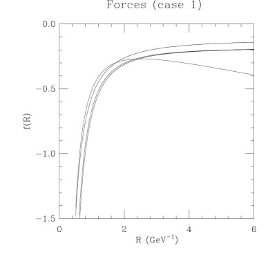
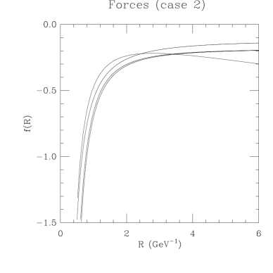
Figure 1:  Plot of: (i) our force $f(R)$ in the $SU(3)$ case (the curve which is decreasing at large $R$), (ii) the forces (for the $c{\overline{c}}$ and the $b{\overline{b}}$ cases) derived from the Cornell potential (the two curves very close to each other), and (iii) the Richardson force (the highest curve). In the first case we set the length scale by using Sommer’s proposal (17), while in the second case we use the condition (20).

References

- [1] D. Zwanziger, Lattice Coulomb Hamiltonian and Static Color-Coulomb Field, hep-th/9603203.
- [2] N. Christ and T. D. Lee, Phys. Rev. D22 (1980) 939.
- [3] A. Cucchieri and D. Zwanziger, Static Color-Coulomb Force, hep-th/9607224, NYU-ThPhCZ7-22-96 preprint.
- [4] M. Baker, J. S. Ball and F. Zachariasen, Nucl. Phys. B186 (1981) 560.
- [5] A. Cucchieri, Numerical results in minimal lattice Coulomb and Landau gauges: color-coulomb potential and gluon and ghost propagators, PhD thesis, New York University (May 1996).
- [6] G. S. Bali and K. Schilling, Nucl. Phys. B (Proc. Suppl.) 34 (1994) 147.
- [7] E. Eichten et al., Phys. Rev. Lett. 34 (1975) 369; E. Eichten et al., Phys. Rev. D21 (1980) 203; E. Eichten and F. Feinberg, Phys. Rev. D23 (1981) 2724.
- [8] J. L. Richardson, Phys. Lett. B82 (1979) 272.
- [9] R. Sommer, Nucl. Phys. B411 (1994) 839.
- [10] A. Billoire, Phys. Lett. B104 (1981) 472.
- [11] Particle Data Group, Review of Particle Properties, Phys. Rev. D50 (1994) 1173.