CERN-TH/96-267

IFUP-TH/62-96

hep-th/9611039

TOWARDS A NON-SINGULAR PRE-BIG BANG COSMOLOGY

M. Gasperini

Theory Division, CERN, CH-1211 Geneva 23, Switzerland

M. Maggiore

Istituto Nazionale di Fisica Nucleare and Dipartimento di Fisica dell’Università,
Piazza Torricelli 2, I-56100 Pisa, Italy

and

G. Veneziano

Theory Division, CERN, CH-1211 Geneva 23, Switzerland

Abstract

We discuss general features of the $\beta$-function equations for spatially flat, $(d+1)$-dimensional cosmological backgrounds at lowest order in the string-loop expansion, but to all orders in $\alpha^{\prime}$. In the special case of constant curvature and a linear dilaton these equations reduce to $(d+1)$ algebraic equations in $(d+1)$ unknowns, whose solutions can act as late-time regularizing attractors for the singular lowest-order pre-big bang solutions. We illustrate the phenomenon in a first order example, thus providing an explicit realization of the previously conjectured transition from the dilaton to the string phase in the weak coupling regime of string cosmology. The complementary role of $\alpha^{\prime}$ corrections and string loops for completing the transition to the standard cosmological scenario is also briefly discussed.

Published in Nucl. Phys. B 494, 315 (1997)

CERN-TH/96-267

September 1996

1 Introduction

Standard cosmology [1] assumes that the primordial Universe was in a hot, dense, and highly curved state, very close indeed to the so-called big-bang singularity. By contrast, the duality symmetries of string theory [2, 3, 4] motivate a class of “pre-big bang” cosmological models [3, 5] in which the Universe starts very near the cold, empty and flat perturbative vacuum. This scenario, although theoretically appealing, can only make sense phenomenologically if such unconventional initial conditions evolve naturally into those of the standard scenario at some later time, smoothing out the big-bang singularity. Does this happen?

The early evolution of a Universe that starts at very low curvature and coupling is well described by the low-energy, tree-level string effective action [6, 7]. The corresponding field equations imply that the string perturbative vacuum, with vanishing coupling constant $g_{s}=e^{\phi/2}=0$, is actually unstable towards small homogeneous fluctuations of the metric and the dilaton $\phi$, which can easily ignite an accelerated growth of the curvature and of the coupling [3, 5]. However, in the absence of higher-order corrections to the effective action, such a growth is unbounded: as conjectured in [8] (and later proved to a large extent in [9]), a singularity in the curvature and/or the coupling is reached in a finite amount of cosmic time, for any realistic choice of the (local) dilaton potential. Is such a singularity unavoidable?

Higher-order corrections to the effective action of string theory are controlled by two independent expansion parameters. One is the field-dependent (and thus in principle space-time-dependent) coupling $g_{s}$, which controls the importance of string-loop corrections. The other parameter, $\alpha^{\prime}$, controls the importance of finite-string-size corrections, which are small if fields vary little over a string-length distance $\lambda_{s}=\sqrt{\alpha^{\prime}}$. Only when this second expansion parameter is small, can the higher-derivative corrections to the action be neglected and does string theory go over to an effective quantum field theory.

As discussed in previous examples [10]-[13], quantum corrections arising in the strong coupling regime can regularize the curvature singularity of the tree-level pre-big bang models, already at the one-loop order. With the exception of the very particular case of two space-time dimensions, the inclusion of loops is necessarily associated with the appearance of higher-derivative terms in the effective action, and thus requires also, for consistency, the inclusion of higher orders in $\alpha^{\prime}$. Instead, if the initial value of the string coupling is small enough, it is quite possible that the Universe reaches the high-curvature regime in which higher-derivative ($\alpha^{\prime}$) corrections become important, while the coupling is still small enough to neglect loop corrections.

According to the above considerations, we shall discuss hereafter the regularization of the curvature singularity just as a result of “stringy” $\alpha^{\prime}$ corrections, but at lowest order in $g_{s}$. We will consider, in particular, the possibility that a cosmological background evolving from the perturbative vacuum be attracted into a state of constant curvature and linearly running dilaton, i.e. of constant $H$ and $\dot{\phi}$ ($H=\dot{a}/a$ is the Hubble parameter in the so-called string frame, i.e. in the frame most directly related to the $\sigma$-model parametrization of the action, and the dot stands for differentiation with respect to cosmic time in that frame).

A high-curvature string phase with frozen string-size values of $H$ and $\dot{\phi}$ was previously conjectured as a crucial ingredient for a successful pre-big bang scenario, and has important phenomenological consequences [14]. Such a state exists in general as a cosmological solution of higher-curvature effective actions, but is in general disconnected from the perturbative vacuum (the trivial solution with $H=\dot{\phi}=0$) by a singularity, or by an unphysical region in which $H$ becomes imaginary. String theory, on the contrary, provides examples in which the two states are smoothly joined by the evolution of the background already to first order in $\alpha^{\prime}$, as we will show in this paper. In this sense string theory automatically implements, without a scalar potential and in any number of dimensions, the “limiting curvature” hypothesis previously introduced ad-hoc, with various mechanisms [15, 16], to regularize the curvature of cosmological backgrounds.

A final state with linearly evolving dilaton can also be obtained in the context of one-loop-regularized models. The main difference between the loop case and the one at hand is that our final shifted dilaton $\overline{\phi}$ satisfies, in $d$ isotropic spatial dimensions, $\dot{\overline{\phi}}\equiv\dot{\phi}-dH<0$. This is a necessary condition for the background to be subsequently attracted by an appropriate potential in a state with expanding metric ($H>0$) and frozen dilaton ($\dot{\phi}=0$), the starting point of standard cosmology. In fact, since the dilaton keeps growing after the transition to the string phase, the effects of loops, of a non-perturbative dilaton potential, and of the back-reaction from particle production must eventually become important, and are expected to play an essential role in the second transition from the string phase to the usual hot big bang scenario. Leaving this second transition to further investigation, the main purpose of this paper is to give arguments in favour of the occurrence of a smooth evolution, in the weak coupling regime, from the dilaton phase to the constant curvature string phase dominated by the $\alpha^{\prime}$ corrections.

The paper is organized as follows. In Section 2 we discuss the general structure of tree-level, $\sigma$-model $\beta$-functions for generic Bianchi-type I backgrounds (including a time-dependent dilaton). In Section 3 we specialize the equations to the case of constant curvature and linear dilaton, and show that in this case we obtain a system of $(d+1)$ algebraic equations in $(d+1)$ unknowns ($d$ Hubble constants and $\dot{\phi}$). The equations look like those for the fixed points of a renormalization group (RG) flow in physical cosmic time (as opposed to the RG “time”). In Section 4 we consider an example to first order in $\alpha^{\prime}$ (i.e. four derivatives), determine the fixed points, and show, by numerical integration, that any isotropic pre-big bang background necessarily evolves smoothly towards the regular fixed points, thus avoiding the singularity. The fixed points have in general an attraction basin of finite area, in the space of initial conditions, also for anisotropic backgrounds. Section 5 contains our conclusions.

2 Bianchi I tree-level $\beta$-functions

It is well known [6, 7] that the field equations for the background fields appearing in the $\sigma$-model action of string theory correspond to the vanishing of a set of $\beta$-function(al)s. We shall call the latter “$\sigma$-model $\beta$-functions” in order to avoid a possible confusion with another set of effective $\beta$-functions to be introduced later. It is also known [6, 7] that the $\sigma$-model $\beta$-functions vanish on a set of field equations that can be derived by varying a space-time effective action $\Gamma$, which is also the generating functional of the string $S$-matrix.

We shall consider in this paper a $\sigma$-model background in ($d+1$) dimensions, consisting of just a time-dependent dilaton $\phi(t)$ and an anisotropic Bianchi-type I metric, $g_{\mu\nu}$, which can be conveniently parametrized as:

$$g_{\mu\nu}={\rm diag}\left(N^{2}(t),-a_{i}^{2}(t)\delta_{ij}\right);~{}~{}~{}~{}~{}~{}~{}~{}i,j=1,...,d.$$ (2.1)

Here $N(t)$ is the lapse function and $a_{i}(t)$ are the scale factors along the $d$ different spatial directions. We will not consider, for the sake of simplicity, an additional antisymmetric-tensor background $B_{\mu\nu}$, which is needed in order to discuss the $O(d,d)$ symmetries [17, 18] associated with the presence of $d$ Abelian isometries, but our considerations can easily be extended to such a case.

Using the general covariance of the string effective action and the fact that, at tree-level in the string-loop expansion, the dependence on a constant dilaton is fixed in the string frame, we can immediately write the exact, tree-level effective action for this background, in terms of the fields

$$\overline{\phi}=\phi-\sum_{i}\beta_{i},~{}~{}~{}~{}~{}~{}~{}~{}~{}~{}\beta_{i}=\ln~{}a_{i},$$ (2.2)

in the form:

$$\Gamma=\int dtNe^{-\overline{\phi}}{\rm L}\left(\dot{\beta}_{i}^{(n)},\dot{\overline{\phi}}_{i}^{(n)}\right).$$ (2.3)

The effective Lagrangian $\rm{L}$ is a general function of the (properly covariantized) time derivatives of the fields $\beta_{i}$ and $\overline{\phi}$, at all orders in $n\geq 1$:

$$\dot{\beta}_{i}^{(n)}=\prod_{k=1}^{n}\left({1\over N}{d\over dt}\right)^{k}\beta(t),~{}~{}~{}~{}~{}~{}~{}~{}\dot{\overline{\phi}}^{(n)}=\prod_{k=1}^{n}\left({1\over N}{d\over dt}\right)^{k}\overline{\phi}(t).$$ (2.4)

In this paper we shall limit our attention to the case of critical (super)strings in which no cosmological constant appears in ${\rm L}$. Thus, even when we discuss the case $d\not=d_{{\rm crit}}$ we shall assume that other “passive” sectors are present to cancel the central charge deficit $(d-d_{{\rm crit}})/3\alpha^{\prime}$.

There are just three kinds of $\sigma$-model $\beta$-function equations that follow from (2.3). They correspond, respectively, to the field equation for the lapse, for each scale factor, and for the dilaton $\overline{\phi}$. However, these ($d+1$) equations are not independent. The relation among them follows from the general fact that, in a theory with coordinate reparametrization invariance, the set of “non-dynamical” field equations representing constraints on the initial data are covariantly conserved [1], as a consequence of the Bianchi identities. In our particular case, the residual time reparametrization invariance implies the relation:

$$\dot{\beta_{i}}{\delta\Gamma\over\delta{\beta_{i}}}\;+\dot{\overline{\phi}}{\delta\Gamma\over\delta{\overline{\phi}}}=N{d\over dt}{\delta\Gamma\over\delta N}.$$ (2.5)

On the equations of motion each one of the three terms in eq. (2.5) vanishes separately, so that only $(d+1)$ equations are independent, to all orders, in agreement with a general property of the $\sigma$-model $\beta$-functions [19].

The variation of the action (2.3), in the cosmic time gauge $N=1$, gives rise to the following system of field equations:

$${\partial{\rm L}\over\partial\dot{\beta_{i}}}-e^{\overline{\phi}}{d\over dt}\left(e^{-\overline{\phi}}{\partial{\rm L}\over\partial\ddot{\beta_{i}}}\right)+\dots=e^{\bar{\phi}}Q_{i},$$ (2.6)

$$-\rm{L}-e^{\overline{\phi}}{d\over dt}\left(e^{-\overline{\phi}}{\partial\rm{L}\over\partial\dot{\overline{\phi}}}\right)+e^{\overline{\phi}}{d^{2}\over dt^{2}}\left(e^{-\overline{\phi}}{\partial\rm{L}\over\partial\ddot{\overline{\phi}}}\right)+\dots=0\;,$$ (2.7)

$${\rm L}-\dot{\overline{\phi}}{\partial{\rm L}\over\partial\dot{\overline{\phi}}}-\dot{\beta_{i}}{\partial{\rm L}\over\partial\dot{\beta_{i}}}-2\ddot{\beta_{i}}{\partial{\rm L}\over\partial\ddot{\beta_{i}}}-2\ddot{\overline{\phi}}{\partial{\rm L}\over\partial\ddot{\overline{\phi}}}+e^{\bar{\phi}}{d\over dt}\left(e^{-\bar{\phi}}\dot{\beta_{i}}{\partial{\rm L}\over\partial\ddot{\beta_{i}}}+e^{-\bar{\phi}}\dot{\overline{\phi}}{\partial{\rm L}\over\partial\ddot{\overline{\phi}}}\right)+\dots=0.$$ (2.8)

Equation (2.6), obtained by varying $\beta_{i}$, defines a set of $d$ charges $Q_{i}$ whose conservation follows from the fact that $\Gamma$ depends only upon derivatives of the $\beta_{i}$. The second equation is the (shifted) dilaton equation, while the last equation is the so-called Hamiltonian constraint, following from the variation of the lapse. Relation (2.5) can be directly checked at the level of eqs. (2.6)–(2.8).

Equation (2.5) can be exploited in several ways when solving the system (2.6)–(2.8). The first way, which we adopt here, is to solve the first two equations and to impose the constraint only on the initial data. After solving the equations numerically, we can double check that the constraint remains valid at all times. Alternatively, we can just use the constraint and the conservation equations and ignore the dilaton equation. Equation (2.5) then guarantees that the dilaton equation is automatically satisfied provided $\dot{\overline{\phi}}$ is not identically zero.

3 The constant curvature case

Let us now consider a very special class of backgrounds, those with constant curvature and a linear dilaton, $\dot{\beta}_{i}$ and $\dot{\overline{\phi}}$ constant, where the fields are referred to the so-called string frame defined by the action (2.3). In our coordinate system they correspond to the ansatz:

$$ds^{2}=dt^{2}-\sum_{i}e^{2H_{i}t}dx^{i}dx^{i},~{}~{}~{}~{}~{}~{}~{}\phi(t)=ct+\phi_{0}$$ (3.1)

parametrized by the $(d+1)$ constants $c$ and $H_{i}$.

The only known (all-order) solutions of this type have a trivial Minkowski metric and a constant or linear dilaton [20] depending on whether $d=d_{\rm{crit}}$ or $d>d_{{\rm crit}}$. The existence of other high-curvature solutions of this type is all but excluded [21], however, provided the dilaton is not a constant, $c\not=0$. Note, incidentally, that it is quite crucial that one looks at constant curvature solutions in the string frame [21]. Because of the dilaton’s time-dependence this is not equivalent to a constant curvature in the Einstein frame, for which no-go theorems probably apply [22]. Let us thus discuss the necessary and sufficient conditions for the existence of solutions of this type, which, in accordance with previously used terminology [14], we will term string-phase solutions.

It is clear, by inspection, that, for this class of backgrounds, eqs. (2.6)–(2.8) reduce to $(d+2)$ algebraic equations in the $(d+1)$ unknowns $H_{i}$ and $c$. However, as already discussed, only $(d+1)$ equations are really independent, giving rise to the hope that isolated solutions other than the already mentioned trivial ones might exist. Actually, from eq. (2.6), we easily see that the l.h.s. is constant for a string-phase solution. Thus, in order for the r.h.s. to be constant as well, two possibilities exist: either $\overline{\phi}$ itself is constant with $Q_{i}$ arbitrary, or $Q_{i}=0$ for all $i$. Let us discuss these two possibilities in turn:

• $\dot{\overline{\phi}}\equiv 0$.

  This case looks more attractive at first sight. However, with $\dot{\overline{\phi}}\equiv 0$, the remaining two equations are independent (see discussion in the previous Section) and give two constraints among the $d$ conserved charges $Q_{i}$. Since these charges are already related by the initial (pre-big bang) conditions, fine-tuned initial conditions would be needed in order to flow into a string phase of this kind. For this reason we will concentrate here on the second alternative.

• $\dot{\overline{\phi}}\not=0,\;Q_{i}=0$.

  This case looks at first even worse because, instead of having two constraints among the $d$ conserved charges, we now have set all of them to zero while they are certainly non-vanishing on the pre-big bang solution. However, if $\dot{\overline{\phi}}<0$, both sides of eq.(2.6) will go exponentially to zero at late times, irrespectively of the $Q_{i}$’s. Therefore, as we shall see explicitly in the following section, string-phase solutions with $\dot{\overline{\phi}}<0$ can play the role of late-time attractors for solutions coming from pre-big bang initial conditions.

Although $\dot{\overline{\phi}}<0$ is a necessary condition for the above phenomenon to occur, it turns out not to be always sufficient. This can be most easily understood by using a RG description. Our differential equations (2.6)–(2.8) define a set of RG equations in physical (cosmic) time where $\dot{\overline{\phi}}$, $\dot{\beta_{i}}$ play the role of running couplings. Time-derivatives of the couplings define some new kind of $\beta$-functions whose zeros correspond to the constant-curvature, linear-dilaton fixed points. Trivial Minkowski space (with $\dot{\overline{\phi}}=0$) corresponds to a trivial quadratic zero of the $\beta$-functions and, consequently, is a late-time (early-time) attractor for post-big bang (pre-big bang) initial conditions.

By contrast, a non-trivial simple zero with $\dot{\bar{\phi}}<0$ is a late-time attractor from any initial condition sufficiently close to it. In order that pre-big bang initial conditions flow to this attractor, it is necessary that no other zeros or singularities separate the trivial fixed point from the non-trivial one. If this is the case, the long-conjectured transition from the dilaton to the string phase does indeed take place. In the next section we shall see explicit examples of such an interesting phenomenon.

4 A first-order example

To the first order in $\alpha^{\prime}$, and in the string frame, the simplest effective action that reproduces the massless bosonic sector of the tree-level string $S$-matrix can be written in the form [7]:

$$S=-{1\over 2\lambda_{s}^{d-1}}\int d^{d+1}x\sqrt{|g|}e^{-\phi}\left[R+(\nabla\phi)^{2}-{k\alpha^{\prime}\over 4}R_{\mu\nu\alpha\beta}^{2}\right]\;,$$ (4.1)

where $k=1,1/2$ for the bosonic and heterotic string, respectively (remember that we have assumed the torsion background to be trivial). The corresponding field equations are equivalent, in the sense discussed in [7], to the conditions of $\sigma$-model conformal invariance represented by the vanishing of the $\beta$-functions.

In order to discuss cosmological solutions, it is convenient to perform a field redefinition (preserving, however, the $\sigma$-model parametrization of the action) that eliminates terms with higher than second derivatives from the effective equations. This can be easily done, as is well known, by replacing the square of the Riemann tensor with the Gauss–Bonnet invariant [23] $R^{2}_{GB}\equiv R_{\mu\nu\alpha\beta}^{2}-4R_{\mu\nu}^{2}+R^{2}$, at the price of introducing dilaton-dependent $\alpha^{\prime}$ corrections. The field redefinition

$$\tilde{g}_{\mu\nu}=g_{\mu\nu}+4k\alpha^{\prime}\left[R_{\mu\nu}-\partial_{\mu}\phi\partial_{\nu}\phi+g_{\mu\nu}(\nabla\phi)^{2}\right],~{}~{}~{}\tilde{\phi}=\phi+k\alpha^{\prime}\left[R+(2d-3)(\nabla\phi)^{2}\right],$$ (4.2)

truncated to first order in $\alpha^{\prime}$, leads in particular to the following simple form of the action (dropping the tilde over the redefined fields):

$$S=-{1\over 2\lambda_{s}^{d-1}}\int d^{d+1}x\sqrt{|g|}e^{-\phi}\left[R+(\nabla\phi)^{2}-{k\alpha^{\prime}\over 4}\left(R^{2}_{GB}-(\nabla\phi)^{4}\right)\right],$$ (4.3)

which we will use throughout this section.

We have explicitly checked that the results of this section are qualitatively reproduced also by using different parametrizations of the string effective action, for instance the one obtained by transforming into the string frame a pure Gauss–Bonnet action in the Einstein frame. Such results are not invariant, however, under field redefinitions that are truncated by keeping first order terms in $\alpha^{\prime}$ in the effective action. With an additional truncated redefinition we can in fact modify eq.(4.3), without re-indroducing second derivatives, and obtain, in particular, the special action that was shown to be off-shell equivalent to the conditions of $\sigma$-model conformal invariance [24] through Zamolodchikov-like equations. The same action has also been recently proposed as the correct one to achieve a higher-order extension of the T-duality symmetry [25]. Such an action does have fixed points; however, these are not smoothly connected to the perturbative vacuum. This field-redefiniton dependence of the background properties is unavoidable as long as the $\alpha^{\prime}$ expansion is truncated at a given finite order.

We specialize the Bianchi I background, for simplicity, to the case in which the spatial sections are the product of two isotropic, conformally flat (“external” and “internal”) manifolds, respectively $d$- and $n$-dimensional, described by the metric

$$g_{00}=N^{2}(t),~{}~{}~{}~{}g_{ij}=-\delta_{ij}e^{\beta(t)},~{}~{}~{}~{}g_{ab}=-\delta_{ab}e^{\gamma(t)},~{}~{}~{}~{}i,j=1,...,d;~{}~{}~{}~{}a,b=d+1,...,d+n$$ (4.4)

(note that the total number of spatial dimensions, previously denoted by $d$, is now redefined to be $d+n$). After integration by parts, the action (4.3) can be written as

$$S\propto\int dte^{d\beta+n\gamma-\phi}\left[{1\over N}\left(-\dot{\phi}^{2}-d(d-1)\dot{\beta}^{2}-n(n-1)\dot{\gamma}^{2}-2dn\dot{\beta}\dot{\gamma}+2d\dot{\beta}\dot{\phi}+2n\dot{\gamma}\dot{\phi}\right)+\right.$$

$$\left.{k\alpha^{\prime}\over 4N^{3}}\left(c_{1}\dot{\beta}^{4}+c_{2}\dot{\gamma}^{4}+c_{3}\dot{\phi}\dot{\beta}^{3}+c_{4}\dot{\phi}\dot{\gamma}^{3}+c_{5}\dot{\phi}\dot{\beta}\dot{\gamma}^{2}+c_{6}\dot{\phi}\dot{\beta}^{2}\dot{\gamma}+c_{7}\dot{\beta}^{2}\dot{\gamma}^{2}+c_{8}\dot{\beta}\dot{\gamma}^{3}+c_{9}\dot{\beta}^{3}\dot{\gamma}-\dot{\phi}^{4}\right)\right]\;,$$ (4.5)

where

$$c_{1} = -{d\over 3}(d-1)(d-2)(d-3),~{}~{}c_{2}=-{n\over 3}(n-1)(n-2)(n-3),$$

$$c_{3} = {4\over 3}d(d-1)(d-2),~{}~{}c_{4}={4\over 3}n(n-1)(n-2),~{}~{}c_{5}=4dn(n-1),~{}~{}c_{6}=4dn(d-1),$$

$$c_{7} = -2dn(d-1)(n-1),~{}c_{8}=-{4\over 3}dn(n-1)(n-2),~{}c_{9}=-{4\over 3}dn(d-1)(d-2).$$ (4.6)

Here we are working, for convenience, with the original dilaton $\phi$, but the action can be easily converted to the general form of section 2 using the definition $\phi\equiv\overline{\phi}+d\beta+n\gamma$.

Let us first look for constant curvature solutions in the isotropic case $n=0$. By varying the action with respect to $\phi$ and $N$, and setting $\dot{\phi}=x={\rm const}$, $\dot{\beta}=y={\rm const}$, in the gauge $N=1$, we get the two independent algebraic equations

$$x^{2} + d(d-1)y^{2}-2dxy-{k\alpha^{\prime}\over 4}\left(c_{1}y^{4}+c_{3}xy^{3}-x^{4}\right)-$$

$$- (dy-x)\left[-2x+2dy+{k\alpha^{\prime}\over 4}\left(c_{3}y^{3}-4x^{3}\right)\right]=0,$$

$$x^{2} + d(d-1)y^{2}-2dxy-{3\over 4}k\alpha^{\prime}\left(c_{1}y^{4}+c_{3}xy^{3}-x^{4}\right)=0.$$ (4.7)

We have explicitly checked that they have real solutions for any $d$ from $1$ to $9$. For $d=3,6,9$, in particular, the coordinates of the fixed point in the plane $(\dot{\phi},\dot{\beta})$ are given by (in units $k\alpha^{\prime}=1$)

$$d = 3~{}~{}~{}~{}~{}~{}~{}~{}~{}~{}x=\pm 1.40...,~{}~{}~{}~{}~{}~{}y=\pm 0.616...,$$

$$d = 6~{}~{}~{}~{}~{}~{}~{}~{}~{}~{}x=\pm 1.37...,~{}~{}~{}~{}~{}~{}y=\pm 0.253...,$$

$$d = 9~{}~{}~{}~{}~{}~{}~{}~{}~{}~{}x=\pm 1.38...,~{}~{}~{}~{}~{}~{}y=\pm 0.163...,~{}~{}.$$ (4.8)

Exactly the same results follow from the system of equations obtained by varying $\{N,\beta\}$ and $\{\phi,\beta\}$. In the last case one gets an additional fixed point, which corresponds, however, to $\dot{\overline{\phi}}=x-dy=0$. In that case the third equation is no longer a consequence of the other two: indeed, by imposing the constraint $\delta S/\delta N=0$, one finds that the additional solution has to be discarded, in agreement with the general discussion of the previous sections. Although we have not made an exhaustive search, it seems that non-isotropic fixed points are excluded in the absence of an exact duality symmetry.

By integrating numerically the field equations for $\beta$ and $\phi$, and imposing the constraint on the initial data, we have verified that, for any given initial condition corresponding to a state of pre-big bang evolution from the vacuum (i.e. $0<\dot{\beta}<x$, $\dot{\overline{\phi}}=\dot{\phi}-d\dot{\beta}>0$), the solution is necessarily attracted to the expanding fixed points (4.8). This is illustrated in Fig. 1, for various numbers of dimensions.

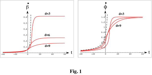
Figure 1: Curvature regularization of a pre-big bang background as a consequence of the first-order $\alpha^{\prime}$ corrections (in units $k\alpha^{\prime}=1$). The dashed curve shows the singular behaviour of the zeroth-order solution in $d=9$. The solid curves approach asymptotically the constant values of eq. (4.8).

In spite of the fact that the fixed points generically appear when higher curvature terms are added to the action, they cannot always be reached from the perturbative vacuum, because of an intermediate singularity or of an unphysical, classically impenetrable region. This is what happens, for instance, if one considers the previously discussed action with the Gauss–Bonnet term alone, which does not correspond, in the string frame, to the correct string effective action. The Gauss–Bonnet invariant, by itself, may parametrize the first-order $\alpha^{\prime}$ corrections only in the Einstein frame, and only in $d=3$ [7].

For the string effective action (4.3), on the contrary, the fixed points are continuously joined to the perturbative vacuum ($\dot{\beta}=0=\dot{\phi}$) by the smooth flow of the background in cosmic time, as illustrated by the “$\beta$-functions” $\ddot{\beta}(\dot{\beta})$, $\ddot{\phi}(\dot{\phi})$ plotted in Fig. 2 ($\dot{\phi}$ and $\dot{\beta}$ are obviously not independent, being related by the constraint equation). They show the running of the curvatures $\dot{\beta}$, $\dot{\phi}$ for the numerical solutions of Fig. 1. The simple action (4.3) thus implements, already to first order in $\alpha^{\prime}$, a smooth transition from the dilaton phase to the string phase of the pre-big bang scenario, in agreement with previous assumptions [14].

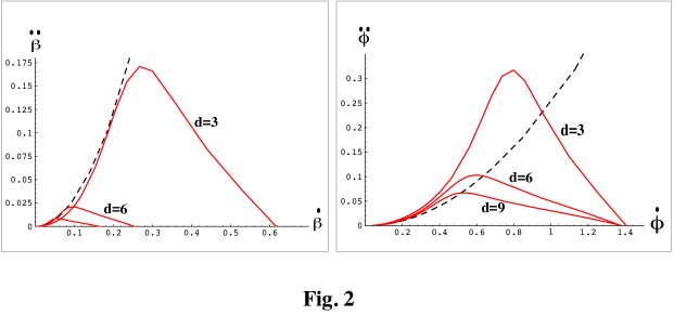
Figure 2: Smooth evolution of the background from the perturbative vacuum, $\dot{\beta}=0=\dot{\phi}$, to the non-trivial fixed points with $\dot{\beta}$ and $\dot{\phi}$ constant reported in eq. (4.8). The dashed curve corresponds to the singular zeroth-order solution.

The contracting fixed points with the negative sign in eq. (4.8) correspond to the time-reversed solutions describing a decelerated, post-big bang contraction, which is also smoothly connected to the perturbative vacuum. The general situation is illustrated in Fig. 3, which shows the time behaviour of the Hubble factor $\dot{\beta}$ (in units $k\alpha^{\prime}=1$) for the case of $d=3$ spatial dimensions. The dashed curves represent the various branches of the singular zeroth-order solution [5]:

$$\sqrt{d}\dot{\beta}=\pm|t|^{-1},~{}~{}~{}~{}~{}~{}~{}~{}~{}~{}~{}~{}~{}\dot{\overline{\phi}}=\pm|t|^{-1},$$ (4.9)

evolving towards ($(a)$ and $(c)$) or from ($(b)$ and $(d)$) the singularity, expanding ($(a)$ and $(b)$) or contracting ($(c)$ and $(d)$). The position of the singularity has been made to coincide with the origin of the time axis, which thus separates the pre-big bang ($t<0$) from the post-big bang ($t>0$) configurations. The four dashed curves are related by T-duality and time-reversal transformation as follows:

$${\rm T-duality} : ~{}~{}~{}~{}~{}~{}~{}~{}~{}(a)\Longleftrightarrow(c),~{}~{}~{}~{}~{}(b)\Longleftrightarrow(d).$$

$${\rm t-reversal} : ~{}~{}~{}~{}~{}~{}~{}~{}~{}(a)\Longleftrightarrow(d),~{}~{}~{}~{}~{}(b)\Longleftrightarrow(c).$$ (4.10)

The numerical integration shows that, at least according to the model (4.3), only expanding pre-big bang and contracting post-big bang configurations are regularized, to first order in $\alpha^{\prime}$, as illustrated by the solid curves. In the context of a theory that is exactly duality-invariant, one may expect, however, a more symmetric situation in which the symmetry pattern of the zeroth-order solutions is maintained after regularization.

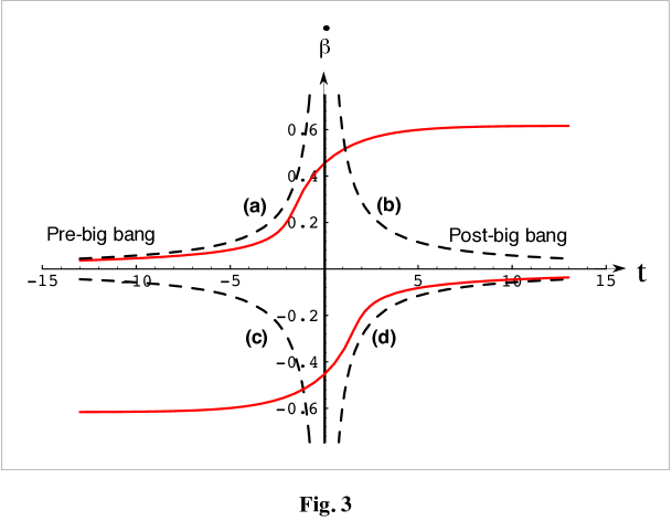
Figure 3: First-order $\alpha^{\prime}$ corrections (solid curves) to the branches of the singular zeroth-order solution (dashed curves).

Since in the present example the dual of the expanding pre-big bang branch is not regularized, no smooth monotonic evolution from growing to decreasing curvature is possible, unlike in models where one-loop corrections are included [10]–[13]. In the loop case, however, the final state of the background tends to remain in the pre-big bang sector with $\dot{\overline{\phi}}>0$, $\dot{\beta}>0$, because of the final growing rate of the dilaton. The expanding fixed point determined by the $\alpha^{\prime}$ corrections corresponds instead to a final configuration of the post-big bang type, with $\dot{\overline{\phi}}<0$, $\dot{\beta}>0$, as illustrated in Fig. 4 by a numerical integration of the $d=3$ field equations. This means that, unlike what happens in the one-loop model of [13], it is not impossible for the background to be attracted by an appropriate potential in the expanding, frozen-dilaton state of the standard scenario.

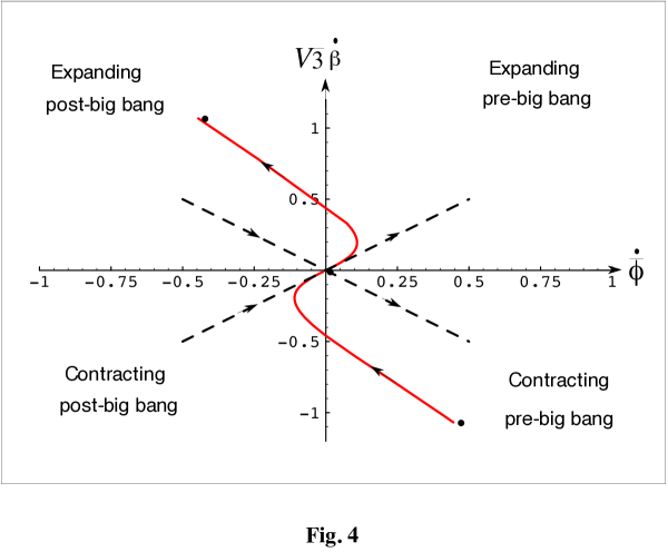
Figure 4: Evolution from the perturbative vacuum to the expanding fixed point (and its time-reversal) to first order in $\alpha^{\prime}$. The dashed lines represent the zeroth-order pre- and post-big bang solutions.

Let us finally stress, to conclude the discussion of our example, that if we start with sufficiently anisotropic initial conditions, the background in general evolves towards a curvature singularity. However, the isotropic fixed points may also attract anisotropic backgrounds, and the set of anisotropic configurations that are eventually attracted by the isotropic fixed point spans a region of finite size in the space of initial conditions. This property of the first-order action (4.3) is illustrated in Fig. 5, where we have plotted various curves $\dot{\gamma}(t)$ and $\dot{\gamma}(\dot{\overline{\phi}})$ obtained through a numerical integration by varying the initial conditions of $\dot{\gamma}$, at fixed initial conditions for $\dot{\beta}$. The plots refer to the case $d=2$, $n=1$ and $\dot{\beta}>0$, but they are qualitatively the same for any $d$ and $n$, and can obviously be symmetrically extended to the plane $\dot{\beta}<0$. When the initial conditions are inside the area spanned by the curves shown in the figure, the curvature is isotropized and regularized, otherwise the singularity is not avoided.

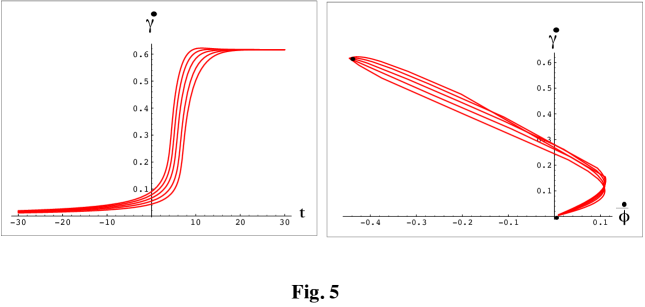
Figure 5: Attraction basin of the fixed points, in the space of anisotropic pre-big bang initial conditions, for the case $d=2$, $n=1$, and for a particular fixed initial value of $\dot{\beta}$.

The size of the attraction basin depends of course on the details of the first-order action. By using, for instance, the $d=3$ effective action obtained by transforming from the Einstein to the string frame the Gauss–Bonnet invariant, we have found a much larger attraction basin than the one illustrated in Fig. 5, so large as to include part of the region $\dot{\gamma}<0$, namely contracting initial conditions. The lack of a complete isotropization is not a negative aspect of the model since, in a higher-dimensional background, the cosmological evolution should indeed implement an effective dimensional reduction by separating three expanding dimensions from the contracting “internal” ones.

5 Conclusions

The evolution of a cosmological background from the string perturbative vacuum may lead to a regime in which higher-derivative contributions to the string effective action are large, while string loop effects are still negligible. We have considered, in that regime, the possible existence of a “string-phase”, with the background curvatures frozen at a scale controlled by the string length parameter $\lambda_{s}$, corresponding to an exponential evolution of the scale factor and a linear evolution of the dilaton (in cosmic time). We have shown that solutions of this kind may represent an exact solution (to all orders in $\alpha^{\prime}$) of the tree-level action, and we have discussed an explicit example (to first order in $\alpha^{\prime}$) in which all expanding isotropic backgrounds, evolving initially from the perturbative vacuum, are necessarily attracted to that constant curvature state.

The main purpose of this paper was to point out the importance of $\alpha^{\prime}$corrections for a singularity-free cosmology: by implementing a mechanism of limiting curvature, they can regularize cosmological backgrounds even in the absence of quantum loop effects. The emergence of such a high-curvature string phase, in the weak coupling regime, leads to a cosmological scenario rich of interesting phenomenological consequences.

In a string-theory context, however, the properties of a background obtained to first order in $\alpha^{\prime}$ (and to any finite order in the $\alpha^{\prime}$ expansion) are characterized by a certain degree of ambiguity [7], because they are not invariant under field redefinitions. A truly unambiguous cosmological background should correspond to the solution of an exact conformal field theory [26], which automatically includes all orders in $\alpha^{\prime}$. In addition, the quantum back-reaction of loops and radiation, as well as an appropriate non-perturbative dilaton potential, are certainly required to complete the transition from the string phase to the radiation-dominated, constant dilaton phase of the standard scenario. In this sense, the results of this paper are still preliminary to the formulation of a complete and realistic string cosmology scenario. Nevertheless, they confirm previous conjectures, clarify the relative role of $\alpha^{\prime}$ and loop corrections, and motivate a more systematic study of higher-order and exact conformal solutions with constant curvature and linear dilatonic evolution.

References

- [1] S. Weinberg, Cosmology and gravitation (Wiley, New York, 1972).
- [2] R. Brandenberger and C. Vafa, Nucl. Phys. B316 (1989) 391.
- [3] G. Veneziano, Phys. Lett. B265 (1991) 287.
- [4] A. A. Tseytlin and C. Vafa, Nucl. Phys. B372 (1992) 443.
- [5] M. Gasperini and G. Veneziano, Astropart. Phys. 1 (1993) 317; Mod. Phys. Lett. A8 (1993) 3701; Phys. Rev. D50 (1994) 2519. An updated collection of papers on the pre-big bang scenario is available at http://www.to.infn.it/teorici/gasperini/.
- [6] C. Lovelace, Phys. Lett. B135 (1984) 75; E. S. Fradkin and A. A Tseytlin, Nucl. Phys. B261 (1985) 1; C. G. Callan et al., Nucl. Phys. B262 (1985) 593; A. Sen, Phys. Rev. Lett. 55 (1985) 1846.
- [7] R. R. Metsaev and A. A. Tseytlin, Nucl. Phys. B293 (1987) 385.
- [8] R. Brustein and G. Veneziano, Phys. Lett. B329 (1994) 429.
- [9] N. Kaloper, R. Madden and K. A. Olive, Nucl. Phys. B452 (1995) 677; Phys. Lett. B371 (1996) 34; R. Easther, K. Maeda and D. Wands, Phys. Rev. D53 (1996) 4247.
-
[10]
I. Antoniadis, J. Rizos and K. Tamvakis,
Nucl. Phys. B415 (1994) 497;
J. Rizos and K. Tamvakis, Phys. Lett. B326 (1994) 57. - [11] R. Easther and K. Maeda, One-loop superstring cosmology and the non-singular universe, hep-th/9605173, Phys. Rev. D, in press.
- [12] S. J. Rey, Phys. Rev. Lett. 77 (1996) 1929.
- [13] M. Gasperini and G. Veneziano, Phys. Lett. B387 (1996) 715.
- [14] R. Brustein, M. Gasperini, M. Giovannini and G. Veneziano, Phys. Lett. B361 (1995) 45; M. Gasperini, M. Giovannini and G. Veneziano, Phys. Rev. Lett. 75 (1995) 3796; M. Gasperini, in “String gravity and physics at the Planck energy scale”, ed. by N. Sanchez and A. Zichichi (Kluwer Acad. Pub., Dordrecht, 1996), p. 305; R. Brustein, M. Gasperini and G. Veneziano, Peak and end point of the relic gravitaton background in string cosmology, CERN-TH/96-37 (hep-th/9604084); A. Buonanno, M. Maggiore and C. Ungarelli, Spectrum of relic gravitational waves in string cosmology, IFUP-TH 25/96 (gr-qc/9605072).
- [15] M. Gasperini, in “Advances in theoretical physics”, ed. by E. R. Caianiello (World Scientific, Singapore, 1991), p. 77.
- [16] V. Mukhanov and R. Brandenberger, Phys. Rev. Lett. 68 (1992) 1969.
- [17] K. A. Meissner and G. Veneziano, Mod. Phys. Lett. A6 (1991)3397; Phys. Lett. B267 (1991) 33; M. Gasperini and G. Veneziano, Phys. Lett. B277 (1992) 256.
- [18] A. Sen, Phys. Lett. B271 (1991) 295; S. F. Hassan and A. Sen, Nucl. Phys. B375 (1992) 103.
- [19] G. Curci and G. Paffuti, Nucl. Phys. B286 (1987) 399.
- [20] C. Myers, Phys. Lett. B199 (1987) 371.
- [21] M. Gasperini and M. Giovannini, Phys. Lett. B287 (1992) 56.
- [22] D. G. Boulware and S. Deser, Phys. Lett. B175 (1986) 409; S. Kalara, C. Kounnas and K. A. Olive, Phys. Lett. B 215 (1988) 265; S. Kalara and K. A. Olive, Phys. Lett. B218 (1989) 148.
- [23] B. Zwiebach, Phys. Lett. B156 (1985) 315.
- [24] N. E. Mavromatos and J. L. Miramontes, Phys. Lett. B201 (1988) 473.
- [25] K. A. Meissner, Symmetries of higher-order string gravity actions, CERN-TH/96-291 (hep-th/9610131).
- [26] E. Kiritsis and C. Kounnas, Phys. Lett. B331 (1994) 51.