CERN-PH-TH/2006-211
F-term uplifting via consistent D-terms

Abstract

The issue of fine-tuning necessary to achieve satisfactory degree of hierarchy between moduli masses, the gravitino mass and the scale of the cosmological constant has been revisited in the context of supergravities with consistent D-terms. We have studied (extended) racetrack models where supersymmetry breaking and moduli stabilisation cannot be separated from each other. We show that even in such cases the realistic hierarchy can be achieved on the expense of a single fine-tuning. The presence of two condensates changes the role of the constant term in the superpotential, $W_{0}$, and solutions with small vacuum energy and large gravitino mass can be found even for very small values of $W_{0}$. Models where D-terms are allowed to vanish at finite vevs of moduli fields - denoted ‘cancellable’ D-terms - and the ones where D-terms may vanish only at infinite vevs of some moduli - denoted ‘non-cancellable’ - differ markedly in their properties. It turns out that the tuning with respect to the Planck scale required in the case of cancellable D-terms is much weaker than in the case of non-cancellable ones. We have shown that, against intuition, a vanishing D-term can trigger F-term uplifting of the vacuum energy due to the stringent constraint it imposes on vacuum expectation values of charged fields. Finally we note that our models only rely on two dimensionful parameters: $M_{P}$ and $W_{0}$.

1 Introduction

The issue of hierarchical supersymmetry breakdown and moduli stabilisation returns as one of the leading themes in superstring phenomenology. One needs to create a potential for various moduli fields which should simultaneously break supersymmetry, split masses of superpartners in observable sector, and fix the remaining parameters of the low energy Lagrangian. Selecting the right vacuum is made more difficult by the existence of a trivial vacuum in stringy models, corresponding to a noninteracting theory. To make the low-energy vacuum stable one needs to make the barrier between the finite and trivial vacua sufficiently high and steep, which in particular implies that the masses of the moduli, like the dilaton and the volume modulus, should be notably larger than the TeV scale (which is also the scale of the gravitino mass in scenarios with gravity mediation). In addition, the scale of the vacuum energy has to be realistically small, orders of magnitude below the TeV scale.

The last requirement is particularly difficult to fulfil, as in generic models of spontaneous supergravity breaking the vacuum energy tends to become negative, of the order $m_{3/2}^{2}M_{P}^{2}$.

There are a limited number of options to uplift the vacuum energy to make it vanish or slightly positive. Firstly, one may add an uplifting term which explicitly breaks local supersymmetry. This route has been known as the KKLT scenario, [1, 2], and has been widely explored by many authors. Secondly, the uplifting could be supersymmetric, if one finds a way to cancel the negative definite term $-3e^{K}|W|^{2}$ in the SUGRA scalar potential by a) $1/2g^{2}D^{2}$ – D-term uplifting or b) $e^{K}K_{i\bar{j}}F^{i}\bar{F}^{\bar{j}}$ – F-term uplifting. The first option has been explored in [3, 4, 5, 6, 7], and, in [5, 6], it was found that with a single non-perturbative sector, the cancellation of the cosmological constant by the D-term while keeping hierarchically small gravitino mass is possible provided certain fine-tuning can be accepted and suitable corrections to the Kähler potential of the volume modulus are introduced. Otherwise, as noted earlier in [3, 8, 9] one tends to obtain a heavy modulus and either a very heavy gravitino mass or an excessively large cosmological constant.

An example of F-term cancellation is no-scale supergravity, which however doesn’t stabilise the no-scale modulus at tree level. A way out of this problem has been proposed in [10] and further explored in [11], where a D-term was suggested as an additional contribution fixing the value of the no-scale modulus. A general study of F-term uplifting given by [12] demonstrated that if supersymmetry is broken by F-terms from a sector that is not strongly influenced by gravity, the SUSY breaking sector can act as an uplifting potential. In fact, it has been subsequently shown that uplifting and simultaneous stabilisation due solely to the F-terms is possible in simple cases of the O’Raifeartaigh type [13], with ISS-type [14] or Polonyi hidden sectors, considered in [15, 16, 17] and in warped backgrounds [18]. However, tuning is necessary in these models too, and in the supersymmetry breaking sector one needs to give up on the (stringy) feature that all dynamically generated mass scales, which eventually provide explanation of hierarchy between the Planck and the electroweak scales, are moduli dependent.

In this letter we present a refined mechanism of supersymmetric F-term uplifting in the presence of consistent D-terms. We introduce two condensing sectors (thus effectively we are employing the racetrack scheme). This has the advantage that the role of the constant term in the superpotential, $W_{0}$, which is crucial in the schemes with a single condensate, changes, as the two condensates compete with each other and not with the $W_{0}$. In addition we introduce a spectator charged scalar. As a result, we can rather easily, without any dramatic tree-level hierarchy among the dimensionful parameters of the Lagrangian, achieve nearly vanishing positive or negative (or zero) cosmological constant with all moduli stabilised and small gravitino mass. The D-terms vanish at the interesting minima, and the cancellation of the negative $-3e^{K}|W|^{2}$ is realised by the F-terms of the moduli fields with the D-term acting indirectly, but non-trivially, as a constraint on the F-term and superpotential contributions to the potential. The D-term also serves as a source of large contribution to the mass matrix, hence one of the fields becomes very heavy while the others stay light. The existence of a state heavier than the condensation scale is consistent with the fact that stabilisation and cancellation of the vacuum energy result from the interplay between the gauge sector and gravity-suppressed contributions. A distinct feature of the model discussed here is that except $W_{0}$ which serves mainly as a source of mass for the lightest scalar, all scales in the hidden sector are dynamically generated with all gauge couplings explicitly field-dependent, as implied by string theory, in contrast to models with ISS-type hidden sectors, [14], considered in [15, 16], where the crucial mass scale in the hidden sector has been put in arbitrarily.

2 General setup

To start with let us assume for simplicity that the dilaton becomes stabilized and decouples at some scale $M_{s}$ close to the Planck scale, and below $M_{s}$ the superpotential for the light volume modulus takes the form $W=W_{0}+W(T)$, where $W_{0}=\langle W(S)\rangle$. With the simple expression $W(T)=Ae^{-aT}$, one stabilizes the $T$-modulus but with a negative cosmological constant, $V_{0}<0$. This can be remedied by adding in a positive “D-term” contribution $\delta_{D}V$ which depends on $T$ in such a way that a) it makes the $V_{0}$ positive or zero, and b) it doesn’t spoil the stabilization of $T$. In the scenario presented by KKLT it has been assumed that $\delta_{D}V=1/2g^{2}D^{2}$, where $D=1/(T+\bar{T})^{n}$. This can be seen as arising from brane-antibrane forces, but then supersymmetry is explicitly broken in the effective 4d Lagrangian. This makes it difficult to reliably study questions about soft supersymmetry breaking within 4d field theoretical framework [19].

Alternatively, an interesting possibility is that the uplifting term could be a FI term coming from gauging of a shift symmetry [20]. However, as noticed by Dudas et al. [5] the simple superpotential $W=W_{0}-Ae^{-aT}$ is not invariant under the local imaginary shift of $T$: $T\rightarrow T+i\delta/2\Lambda$ which produces D-terms of the required form. It turns out that introducing a gauge invariant version of the superpotential changes the rules of the game. We shall follow this route below, putting aside the possibility of gauging an R-symmetry, see Zwirner et al.[9], Binetruy et al.[21].

2.1 Gauging the shift

In this letter we will limit our focus to models which are invariant under non-R $U(1)$ gauge symmetry. Let us consider gauging of the imaginary shift of the modulus $T$. It has been shown in [22] that one can indeed realise such a situation in stringy models. Let $K=K(T+\bar{T})$. The shift $T\rightarrow T+i\delta/2\Lambda$ is generated by the Killing vector $X_{T}=i\delta/2$ where $\delta$ is real. The prepotential $D$ fulfills the Killing equation $K_{T\bar{T}}\bar{X}=i\partial D/\partial T$, and generates the scalar potential $\delta V=1/2g^{2}D^{2}$. One finds, upon solving the Killing equation, $D=-\frac{\delta}{2}\frac{\partial K}{\partial\bar{T}}+\xi$, where $\xi$ is a genuine constant. If $\xi\neq 0$ the gauged symmetry acts on gravitini and becomes a local $U(1)$ R-symmetry, as described earlier. We shall set $\xi=0$ in what follows. To be consistent with global supersymmetry algebra the superpotential must be invariant under any local (non-R) symmetry. The invariant superpotential which is solely a function of the modulus $T$ must therefore be a constant. This is not sufficient to stabilize the $T$.

The solution is to introduce more charged fields:

$$\delta Z=i\Lambda q_{Z}Z;\;\;X_{Z}=iq_{Z}Z.$$ (1)

2.2 Gaugino condensation

Let us assume that the source of the superpotential for $T$ is non-perturbative effects in a strongly coupled gauge theory. For simplicity let us take $SU(N)$ hidden gauge group with $N_{f}<N$ pairs of $N$ and $\bar{N}$ representations. In addition, let us assume that the fields are charged under a local $U(1)$. Below the condensation scale the effective non-perturbative superpotential is

$$W_{npert}=(N-N_{f})\left(\frac{\Lambda_{cond}^{b_{0}}}{detM}\right)^{\frac{1}{N-N_{f}}},$$ (2)

where $b_{0}=3N-N_{f}$, $M_{ij}=Q_{i}\bar{Q}_{j}$. The condensation scale is related to the modulus $T$ through the relation $\Lambda_{cond}=e^{-T/b_{0}}$ where $Re(T)=\frac{8\pi^{2}}{g^{2}}$. Let us take $N_{f}=1$. Then the superpotential becomes

$$W_{npert}=(N-1)\left(\frac{e^{-T}}{M}\right)^{\frac{1}{N-1}}.$$ (3)

This is invariant under the local $U(1)$ if $M\rightarrow Me^{i(q+\bar{q})\Lambda}$ with $\delta=-2(q+\bar{q})$. In general this means that $Tr(Q_{U(1)})$ is nonzero, so naively it is anomalous. However, the 4d Green-Schwarz mechanism may be employed to cancel the one-loop anomalous diagrams, or one can imagine adding to the model a number of charged fields which do not enter the superpotential.

To be able to write down the effective potential one needs also the Kähler function for the composite meson fields M. Here one should use symmetries. Possible choices are for instance $K=\bar{M}{M}/M_{P}^{2}$ or $K=\sqrt{\bar{M}{M}}$. Since we do not believe that a particular choice of the Kähler potential could play a significant role, we take the first option which leads to cleaner formulae.

3 Racetrack with consistent D-terms

The simplest model that works analogously to the original KKLT model is the one with a racetrack superpotential stabilizing $T$:

$$W=A_{1}N_{1}\left(\frac{e^{-T}}{M_{1}}\right)^{\frac{1}{N_{1}}}-A_{2}N_{2}\left(\frac{e^{-T}}{M_{2}}\right)^{\frac{1}{N_{2}}}+W_{0},$$ (4)

with

$$V_{D}=\frac{\pi^{2}\delta^{2}}{t}(\frac{b}{2t}+x_{1}^{2}+x_{2}^{2})^{2},$$ (5)

where $x_{i}=|M_{i}|\geq 0$. We assume the Kähler function

$$K=-b\log(T+\bar{T})+M_{1}\bar{M}_{1}+M_{2}\bar{M}_{2}\ ,$$ (6)

with $b=1,2\;{\rm or}\;3$. Notice that there could be a constant contribution to the Kähler potential, $c_{K}$, which would rescale uniformly all terms in the scalar potential by $e^{c_{K}}$, except the contribution $V_{D}$. In this respect $c_{K}$ acts in the way analogous to that of the charge $\delta$, which in turn rescales only $V_{D}$. The superpotential is defined up to the overall complex phase. Hence, one can fix that phase in such a way that the constant part of the superpotential ($W_{0}$) can be considered to be a real number. Then the scalar potential takes the form

$$V=V_{F}+V_{W}+V_{D}\ ,$$ (7)

with

$$V_{F}=(2t)^{-b}e^{x_{1}^{2}+x_{2}^{2}}\Bigg{[} |A_{1}|^{2}\left(\frac{e^{-2t}}{x_{1}^{2}}\right)^{\frac{1}{N_{1}}}\left[b\left(\frac{2t}{b}+N_{1}\right)^{2}+x_{1}^{2}\left(N_{1}-\frac{1}{x_{1}^{2}}\right)^{2}+x_{2}^{2}N_{1}^{2}\right]$$

$$+|A_{2}|^{2}\left(\frac{e^{-2t}}{x_{2}^{2}}\right)^{\frac{1}{N_{2}}}\left[b\left(\frac{2t}{b}+N_{2}\right)^{2}+x_{2}^{2}\left(N_{2}-\frac{1}{x_{2}^{2}}\right)^{2}+x_{1}^{2}N_{2}^{2}\right]$$

$$+W_{0}^{2}\left[b+x_{1}^{2}+x_{2}^{2}\right]$$

$$\begin{aligned} -\ 2|A_{1}||A_{2}|\left(\frac{e^{-t}}{x_{1}}\right)^{\frac{1}{N_{1}}}\left(\frac{e^{-t}}{x_{2}}\right)^{\frac{1}{N_{2}}}\cos\left(\phi_{1}-\phi_{2}\right)\Bigg{[}&b\left(\frac{2t}{b}+N_{1}\right)\left(\frac{2t}{b}+N_{2}\right)\\ &+x_{1}^{2}\left(N_{1}-\frac{1}{x_{1}^{2}}\right)N_{2}+x_{2}^{2}\left(N_{2}-\frac{1}{x_{2}^{2}}\right)N_{1}\Bigg{]}\end{aligned}$$

$$+2W_{0}|A_{1}|\left(\frac{e^{-t}}{x_{1}}\right)^{\frac{1}{N_{1}}}\cos\left(\phi_{1}\right)\left[2t+N_{1}b+N_{1}\left(x_{1}^{2}+x_{2}^{2}\right)-1\right]$$

$$-2W_{0}|A_{2}|\left(\frac{e^{-t}}{x_{2}}\right)^{\frac{1}{N_{2}}}\cos\left(\phi_{2}\right)\left[2t+N_{2}b+N_{2}\left(x_{1}^{2}+x_{2}^{2}\right)-1\right]\Bigg{]}\ ,$$ (8)

and

$$V_{W}=-3(2t)^{-b}e^{x_{1}^{2}+x_{2}^{2}}\Bigg{[} |A_{1}|^{2}\left(\frac{e^{-2t}}{x_{1}^{2}}\right)^{\frac{1}{N_{1}}}N_{1}^{2}+|A_{2}|^{2}\left(\frac{e^{-2t}}{x_{2}^{2}}\right)^{\frac{1}{N_{2}}}N_{2}^{2}+W_{0}^{2}$$

$$-2|A_{1}||A_{2}|\left(\frac{e^{-t}}{x_{1}}\right)^{\frac{1}{N_{1}}}\left(\frac{e^{-t}}{x_{2}}\right)^{\frac{1}{N_{2}}}\cos\left(\phi_{1}-\phi_{2}\right)N_{1}N_{2}$$

$$+2W_{0}|A_{1}|\left(\frac{e^{-t}}{x_{1}}\right)^{\frac{1}{N_{1}}}\cos\left(\phi_{1}\right)N_{1}-2W_{0}|A_{2}|\left(\frac{e^{-t}}{x_{2}}\right)^{\frac{1}{N_{2}}}\cos\left(\phi_{2}\right)N_{2}\Bigg{]}\ ,$$ (9)

where $A_{1}=|A_{1}|e^{i\omega_{1}},\;A_{2}=|A_{2}|e^{i\omega_{2}},\;M_{1}=x_{1}e^{i(\phi_{1}+\omega_{1})N_{1}},\;M_{2}=x_{2}e^{i(\phi_{2}+\omega_{2})N_{2}},\;T=t+ia\,$.

At first glance we have 6 degrees of freedom in this model: $t$, $x_{1}$, $x_{2}$, $a$, $\phi_{1}$ and $\phi_{2}$. In fact only 5 of them are relevant: certain combination of $a$ and two phases $\phi_{1}$ and $\phi_{2}$ forms the longitudinal polarisation of the massive gauge boson, that appears due to spontaneous breakdown of the shift symmetry. Hence, one can gauge away one combination of these fields. Alternatively, one may choose to work with a flat direction in the scalar potential. Hence in practice one needs to solve the potential with respect to $t$, $x_{1}$, $x_{2}$, $\phi_{1}$, $\phi_{2}$ and $a$ then the flat direction can be identified with the longitudinal polarisation. In addition, different choices of $\omega_{1}$ and $\omega_{2}$ correspond to the different settings of the origins of the $\phi_{1}$ and $\phi_{2}$ variables respectively. Without lose of generality, one can put $\omega_{1}=\omega_{2}=0$.

The behaviour of this model is close to that of the racetrack, with the $t$ modulus being stabilised by its F-term potential. The minimum appears close to:

$$\left\langle t\right\rangle=\ln\left(\frac{|A_{1}|x_{2}^{1/N_{2}}}{|A_{2}|x_{1}^{1/N_{1}}}\right)\frac{N_{1}N_{2}}{|N_{2}-N_{1}|}$$ (10)

where the dynamical phases absorb any overall phases, such as the sign of $N_{2}-N_{1}$. We expect $x_{1}$ and $x_{2}$ to be typically order one because they have no sources of hierarchy. Hence the minimum reached will not be exactly the value given by Eq. (10) since there are additional contributions to the potential coming from the F-terms for the condensate fields and the D-term. However, for the values of the parameters considered in this paper the differences are minimal.

In addition to $t$, the $x_{1}$ and $x_{2}$ fields need stabilising. To see that this must happen we need only consider $V_{W}$ and $V_{F}$. Since $V_{W}$ only contains negative, fractional powers of $x_{1}$ and $x_{2}$ it is unbounded from below with $x_{1}$ and $x_{2}$ tending to zero. However, $V_{F}$ includes larger negative powers with positive coefficients, coming from the $\frac{\partial W}{\partial x_{i}}$ terms, and the negative singularity is lifted to be a positive singularity. Finally, $x_{1}$ and $x_{2}$ cannot run off to infinity since the F-terms for $M_{1}$ and $M_{2}$ contain positive powers of $x_{1}$ and $x_{2}$ cancelling the negative powers coming from the superpotential.

Since the phases are cyclic, by definition, stability is guaranteed and the number of flat directions is determined by the global symmetries. With all input parameters set to non-zero values there exists one flat direction corresponding to the anomalous $U(1)$ gauge symmetry.

At this stage, the potential is stable without needing to utilise the D-term. It is clear that the D-term contribution alone cannot stabilise $t$ since it runs off to $\infty$, but it does perturb the minimum reached. The importance of the D-term is in cancelling the cosmological constant. Since $V_{D}$ is very flat at large $t$ its effect on the position of the minimum is minor, but it provides a positive definite contribution to $V$, which allows the cosmological constant to be tuned to zero with arbitrary precision. As expected this closely mirrors the behaviour in the original KKLT formulation, with the D-term lifting playing the role of the explicit SUSY breaking anti–D-brane contribution.

In addition to the direct contribution of $V_{D}$’s energy density to $V$, the D-term indirectly increases the overall energy density through its effect on $V_{F}$ and $V_{W}$. Since $V_{F}+V_{W}$ minimise with $\delta=0$ it follows that any alteration of the position of the minimum will increase the value of $V_{F}+V_{W}$ (assuming no flat directions). It is the combination of these two effects that gives rise to the final expectation values minimising the potential.

Unfortunately these effects are too efficient. A very small $\delta\sim 10^{-14}$ is sufficient to lift from a negative to a positive minimum and a natural, order one, $\delta$ does not allow finite minimisation. In principle, from the point of view of the effective field theory a very small effective $U(1)$ charge of $T$ and $M_{i}$ could be tolerable although it is highly unnatural, and it is also unnatural from the point of view of string theory. Thus we shall try to improve the model in such a way that solutions with $\delta\sim 1$ could be found. To this end we consider a cancellable D-term in the next section.

At this point it is instructive to have a closer look at the breaking of the anomalous $U(1)$. The mass terms come from the kinetic part of the Lagrangian

$$\frac{b\delta^{2}}{16t^{2}}(V_{\mu}-\frac{2}{\delta}\partial_{\mu}{\rm Im}(T))^{2}+x_{i}^{2}q^{2}_{M_{i}}(V_{\mu}-\frac{1}{q_{M_{i}}}\partial_{\mu}\phi_{i}N_{i})^{2},$$ (11)

where $M_{i}=x_{i}e^{i\phi_{i}N_{i}}$ and summation over charged fields is understood. One easily finds out that the mass of the vector boson is given by

$$m^{2}_{V}=\frac{8\pi^{2}}{t}\left(\frac{b\delta^{2}}{8t^{2}}+2q^{2}_{M_{i}}x_{i}^{2}\right)=\frac{4\pi^{2}\delta^{2}}{t}(\frac{b}{4t^{2}}+x_{i}^{2}).$$ (12)

It turns out that in the models we consider here the ‘anomalous’ gauge boson is always rather heavy, see table 1.

4 Natural D-terms and natural charges

Since the D-term in the previous model only minimises for $t\rightarrow\infty$, $x_{1}\rightarrow 0$ and $x_{2}\rightarrow 0$ and contains no sources of hierarchy order one values of $t$, $x_{1}$ and $x_{2}$ imply that $V_{D}$ will be order one. With $V_{W}\sim 10^{-32}$, to obtain a physically reasonable gravitino mass it is clear that $V_{D}$ does not obtain a natural vev, as demonstrated by the smallness of $\delta$. One approach to this problem is to introduce a field that appears with a relative minus sign inside the D-term, such that $V_{D}$ can go to zero for natural input parameter values.

The effect of a cancellable D-term is purely the introduction of a constraint on the rest of the potential. In the limit that the solutions to $\frac{\partial V}{\partial Z_{i}}=0$, where $Z_{i}$ runs over all modulus fields, are governed by the first derivatives of $V_{D}$ then the solution to $\frac{\partial V_{D}}{\partial Z_{i}}=0$ can be imposed as a constraint on $V_{F}$ and $V_{W}$ and, to good approximation, $V_{D}=0$. The simplest possible D-term of this form is obtained by introducing one additional matter field, $C$, with the opposite sign charge to the condensing fields. It sufficient to consider an additional field which does not appear in the superpotential, only in $V_{D}$ and $V_{F}$. We choose to consider a canonical Kähler potential for simplicity.

4.1 Additional Charged Matter

As $C$ does not appear in the superpotential it only interacts via the D-term and through the Kähler derivatives, in the F-terms. This leads to a change of $V_{W}\rightarrow e^{c^{2}}V_{W}$ and a change of $V_{F}\rightarrow e^{c^{2}}V_{F}+V_{F}(c)$, where $c=|C|$ and

$$V_{F}(c)=c^{2}e^{K}|W|^{2}=(2t)^{-b}c^{2}e^{c^{2}}e^{x_{1}^{2}+x_{2}^{2}}\Bigg{[} |A_{1}|^{2}\left(\frac{e^{-2t}}{x_{1}^{2}}\right)^{\frac{1}{N_{1}}}N_{1}^{2}+|A_{2}|^{2}\left(\frac{e^{-2t}}{x_{2}^{2}}\right)^{\frac{1}{N_{2}}}N_{2}^{2}+W_{0}^{2}$$

$$-2|A_{1}||A_{2}|\left(\frac{e^{-t}}{x_{1}}\right)^{\frac{1}{N_{1}}}\left(\frac{e^{-t}}{x_{2}}\right)^{\frac{1}{N_{2}}}\cos\left(\phi_{1}-\phi_{2}\right)N_{1}N_{2}$$

$$+2W_{0}|A_{1}|\left(\frac{e^{-t}}{x_{1}}\right)^{\frac{1}{N_{1}}}\cos\left(\phi_{1}\right)N_{1}-2W_{0}|A_{2}|\left(\frac{e^{-t}}{x_{2}}\right)^{\frac{1}{N_{2}}}\cos\left(\phi_{2}\right)N_{2}\Bigg{]}\ .$$ (13)

The D-term potential is given by

$$V_{D}=\frac{\pi^{2}\delta^{2}}{t}\left(\frac{b}{2t}+x_{1}^{2}+x_{2}^{2}-qc^{2}\right)^{2}$$ (14)

where $q$ is the charge of $C$, defined such that $C\rightarrow e^{iq\delta\Lambda}C$ under the anomalous $U(1)$. If $c$ had no potential, besides the D-term, it would simply move such that it was given by $c^{2}=\frac{1}{q}\left(\frac{b}{2t}+x_{1}^{2}+x_{2}^{2}\right)$ and the minimum for $V_{F}+V_{W}$ would be undisturbed. However $c$ has a mass term from its coupling to $|W|^{2}$ and as such is driven towards zero. Exactly how much $c$ changes from the default value is fixed by the interplay between the minimisation of $t$, $x_{1}$ and $x_{2}$ and the minimisation of $c^{2}|W|^{2}$. The deviation is determined by the size of the mass term for the constraint equation, which is in turn given by $\frac{1}{|q|}|W|^{2}$. The smaller $|q|$ is the larger the effective mass term for the constraint equation and hence the further the solution to the equation will be driven from the preferred value of $V_{F}+V_{W}$. Since moving away from this value will increase the vev of $V_{F}+V_{W}$ a small enough charge lifts the cosmological constant to be positive. In addition to this indirect lifting, the extra matter provides a positive contribution to energy density through the mass term $c^{2}|W|^{2}$. However, since $c^{2}|W|^{2}$ is driven to zero this effect is less important than the effect on $V_{F}+V_{W}$ and, alone, is insufficient to cancel $V_{W}$. The combined effects can lift the potential to be small and positive, as shown in our numerical examples.

The cosmological constant can be sent to zero by tuning the input parameters. It is clear from the previous discussion that there exists a value of the charge $q$ that gives $V=0$, but perhaps a more natural parameter to tune is $W_{0}$. Considering a small $W_{0}$ we see that there is a negligible positive contribution proportional to $W_{0}^{2}$, and two terms coupled to cosines of $\phi_{1}$ and $\phi_{2}$. For small $W_{0}$ the $|A_{1}||A_{2}|\cos(\phi_{1}-\phi_{2})$ term dominates and hence enforces $\phi_{1}=\phi_{2}$. Nonetheless $\phi_{1}$ is still free to align such that the coefficient of $W_{0}$ is negative. Thus a model with a small $W_{0}$ will always result in a lower minimum than the same model with $W_{0}=0$. As a result, $W_{0}$ can be tuned such that $V=0$, assuming that a $q$ is chosen such that when $W_{0}=0$ the minimum is positive.

5 Discussion

We present numerical results and provide approximate, analytic justifications of the results seen.

$\begin{array}[]{|c||c|c|}\hline\cr\text{ Data}&\text{ Non-cancellable }&\text{Cancellable}\\ \hline\cr m_{3/2}&227.761&478.142\\ \hline\cr V_{0}^{1/4}&0&0\\ \hline\cr V_{F}^{1/4}&2.13211\times 10^{10}&3.41239\times 10^{10}\\ \hline\cr V_{D}^{1/4}&1.78276\times 10^{10}&2292.40\\ \hline\cr t&732.348&733.325\\ \hline\cr x_{1}&0.169201&0.173619\\ \hline\cr x_{2}&0.208768&0.237810\\ \hline\cr\phi_{1}&\pi&\pi\\ \hline\cr\phi_{2}&\pi&\pi\\ \hline\cr m_{t}&8.213\times 10^{4}&1.630\times 10^{5}\\ \hline\cr m_{a}&8.277\times 10^{4}&1.646\times 10^{5}\\ \hline\cr m_{x_{1}}&1.760\times 10^{3}&3.141\times 10^{2}\\ \hline\cr m_{x_{2}}&2.369\times 10^{3}&2.427\times 10^{17}\\ \hline\cr m_{c}&\text{N/A}&7.853\times 10^{2}\\ \hline\cr m_{\phi_{1}}&4.914\times 10^{2}&6.000\times 10^{2}\\ \hline\cr m_{\phi_{2}}&0&0\\ \hline\cr m_{V}&4.73\times 10^{3}&8.56\times 10^{17}\\ \hline\cr\end{array}$

Table 1: Comparison of the models. The cosmological constant can be tuned to be as small as the numerical precision allows and hence is set to zero.

In the tables $V_{0}=\left\langle V\right\rangle$ is the cosmological constant and all dimensionful quantities are given in GeV except for the field vevs which are quoted in units in which $M_{P}=1$. Finally, note that the masses quoted are not the masses of the fundamental fields, for which the mass matrix is not diagonal. Instead the masses are labelled by the fundamental field that makes up the largest component of that mass eigenstate.

$\begin{array}[]{|c||c|c|}\hline\cr\text{ Data}&\text{ Non-cancellable }&\text{ Cancellable}\\ \hline\cr b&3&3\\ \hline\cr|A_{1}|&2.62&2.62\\ \hline\cr|A_{2}|&0.3&0.3\\ \hline\cr N_{1}&25&25\\ \hline\cr N_{2}&27&27\\ \hline\cr\delta&6.22\times 10^{-15}&1\\ \hline\cr W_{0}&2\times 10^{-12}&2.13\times 10^{-12}\\ \hline\cr q&N/A&1/2\\ \hline\cr\end{array}$

Table 2: Input parameter values.

Figure 1: Minimisation with a non-cancellable D-term. In addition to the total potential, the F-term, D-term and superpotential contributions are plotted. All quantities are given in units where $M_{P}=1$ and all other fields are fixed at their minimum values.

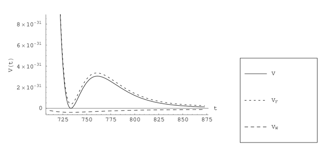
Figure 2: Minimisation with a cancellable D-term. The same potentials are plotted as in figure 1, but with $V_{D}$ removed for clarity and again, $M_{P}=1$ and all other fields are at their minima.

We see that the two models, with similar input parameter values, produce remarkably similar output, but with a few important exceptions. Firstly, $m_{3/2}$ differs markedly between the two models due to the inflation of the potential by $e^{c^{2}}$. Secondly, we see that $m_{x_{2}}$ is many orders of magnitude larger when the D-term is cancellable. This appears because, despite $V_{D}$ and its first derivative being negligible, the second derivative of $V_{D}$ is naturally Planck scale. Notice that the vev of $t$ is essentially the same in both models with the potential having a very similar form as seen in figures 1 and 2. The shows that, since Eq. (10) yields $t=735.816$ and $t=737.096$ for the non-cancellable and cancellable cases respectively, we can conclude that the approximation that the minimum is given by $F_{T}=0$, and hence Eq. (10), is valid for these input parameters.

It is clear that, despite the differences between the models, the fine tuning of $\left\langle V\right\rangle$ to zero can be readily achieved in both cases. The methods of cancellation differ considerably between the two models and it is necessary to consider them separately. Firstly we consider the effect of the cancellable D-term. In this case by setting $W_{0}=0$ and then varying $q$ we see that a small enough charge will lift the potential to be positive. If a small $W_{0}$ is then introduced, the phases will align to ensure that the cross terms produce a negative contribution to the potential (the $W_{0}^{2}$ terms have negligible effect). It has been demonstrated numerically that even small values of $W_{0}$, such as $10^{-11}$, will produce a negative cosmological constant, assuming that $q=1/2$, while $W_{0}=0$ gives $V>0$. Hence for some value of $W_{0}$ in the range $0<W_{0_{c}}<10^{-11}$ it follows that $V=0$ for $W_{0}=W_{0_{c}}$. When varying $W_{0}$ to tune $V$ to zero it is clear that the value of $m_{3/2}$ is essentially independent of the tuning. To be more precise, near $W_{0_{c}}$ the addition of a small $\Delta W_{0}$ will make $V<0$ whereas subtracting $\Delta W_{0}$ will give $V>0$. This will be true in the limit that $\Delta W_{0}\rightarrow 0$, whereas $\Delta m_{3/2}\rightarrow 0$ in this limit. Finally we see that because SUSY is always broken due to the effects of the meson fields $V=0$ has to be obtained by a cancellation between $V_{F}$ and $V_{W}$. This shows that $V=0$ implies a finite $m_{3/2}$ if $t$ stabilises.

In the simple models given here the phase of the field $C$ has no potential whatsoever. However, it is clear that one can add a nontrivial superpotential $\tilde{W}(C)$ to stabilise the phase without affecting stabilisation and cancellation, as long as its expectation value remains smaller than $\langle W\rangle$.

The non-cancellable D-term lifting is both indirect and direct, with the direct lifting from the positive definite contribution to the potential introduced by $V_{D}$. The indirect effect of the non-cancellable D-term is similar to the cancellable D-term’s, the argument of the D-term is driven to zero, which necessarily moves $x_{1}$, $x_{2}$ and $t$ away from the minimum of $V_{F}+V_{W}$ and F-term lifting occurs. In addition to this effect the D-term provides direct lifting analogous to the original KKLT models, with both of these effects being controlled by the size of $\delta$. Hence varying $\delta$ allows the tuning of $V=0$.

Since, in the large $t$ limit, $V_{D}$ is approximately given by $\delta^{2}(x_{1}^{2}+x_{2}^{2})/t$, it is clear that, in this limit, $|\partial V_{D}/\partial t|\ll|V_{D}|$, whereas the exponential dependence of $V_{F}$ ensures that, in this limit, $|\partial V_{F}/\partial t|\sim|\frac{2}{N_{1}}V_{F}|\sim|\frac{2}{N_{2}}V_{F}|$. Since $|V_{F}|$ is of the same order as $|V_{W}|$ and $V$ is tuned to zero, $V_{F}+V_{W}+V_{D}=0$ implies that $V_{D}$ should be of the same order as $|V_{F}|$ and $|V_{W}|$. This, coupled with the fact that $\frac{2}{N_{1}}\gg\frac{1}{t}$, implies that $|\partial V_{F}/\partial t|\gg|\partial V_{D}/\partial t|$. As a result the D-term does not disturb the minimum of $t$. The same is not true for $x_{1}$ and $x_{2}$ since $V_{D}$, $V_{F}$ and $V_{W}$ are all polynomial functions of $x_{1}$ and $x_{2}$ (ignoring the $e^{K}$ factor which is irrelevant to this discussion) and so, very roughly, $\partial V_{F}/\partial x_{i}\sim V_{F}/x_{i}$, $\partial V_{D}/\partial x_{i}\sim V_{D}/x_{i}$ and $\partial V_{W}/\partial x_{i}\sim 0$. This demonstrates that $V_{D}$ and $V_{F}$ have comparable effects on the minima of $x_{i}$ so as a result we expect the minima to shift upon the introduction of $V_{D}$.

6 Summary and outlook

The issue of fine-tuning necessary to achieve satisfactory degree of hierarchy between the moduli masses, gravitino mass and the scale of cosmological constant has been revisited in the context of supergravities with consistent D-terms. We have studied models where supersymmetry breaking and moduli stabilisation cannot be separated from each other: unlike in the models considered in [2, 16] supersymmetry breaking, for finite field vevs, is mandatory. It turns out that even in such a case the realistic hierarchy can be achieved on the expense of a single fine-tuning. In models with cancellable D-terms the tuned parameter turns out to be the constant term in the superpotential, in models with non-cancellable D-term tuning can be restricted to the $U(1)$-charges of moduli. We have studied a refined mechanism of supersymmetric F-term uplifting in the presence of consistent D-terms. We have employed the racetrack scheme enhanced by a constant term in the superpotential. In contrast to the original KKLT construction minimisation is not due to cancellation between $W_{0}$ and the modulus field, but between the separate condensate terms. In addition we introduce a spectator charged scalar. As a result, we can easily, without any dramatic tree-level hierarchy among the dimensionful parameters of the Lagrangian, achieve nearly vanishing positive or negative (or zero) cosmological constant with all moduli stabilised and small gravitino mass. The D-terms vanish at the interesting minima, and the cancellation of the negative $-3e^{K}|W|^{2}$ is realised by the F-terms of the moduli fields. Despite going to zero in the minimum the D-term has a large effect on the mass matrix, inducing a large splitting in the moduli mass spectrum. The existence of a state heavier than the condensation scale is consistent with the fact that stabilisation results from the interplay between the gauge sector and gravity-suppressed contributions. A distinct feature of the model discussed here is that except $W_{0}$, which removes a zero eigenvalue from the mass matrix, all scales in the hidden sector are dynamically generated via running of field dependent gauge couplings, as implied by string theory, in contrast to models with ISS-type hidden sectors considered earlier [15, 16]. Perturbing the model by a small (smaller than $<W>$) superpotential, $\tilde{W}(C)$, for the extra charged scalar doesn’t materially affect the results. Finally, the amount of tuning necessary in the models discussed here is comparable to those in [5, 6, 15, 16].

Acknowledgements

It is a pleasure to thank Stefan Pokorski and Emilian Dudas for helpful discussions.
Z.L. and O.E.-W. thank the CERN Theory Division for hospitality. This work was partially supported by the EC 6th Framework Programme MRTN-CT-2006-035863, by TOK Project MTKD-CT-2005-029466, and by the Polish State Committee for Scientific Research grant KBN 1 P03D 014 26.

References

- [1] S. Kachru, R. Kallosh, A. Linde and S. P. Trivedi, Phys. Rev. D 68 (2003) 046005 [arXiv:hep-th/0301240].
- [2] R. Kallosh and A. Linde, JHEP 0412 (2004) 004 [arXiv:hep-th/0411011].
- [3] A. Achucarro, B. de Carlos, J. A. Casas and L. Doplicher, JHEP 0606 (2006) 014 [arXiv:hep-th/0601190].
- [4] A. P. Braun, A. Hebecker and M. Trapletti, arXiv:hep-th/0611102.
- [5] E. Dudas and S. K. Vempati, Nucl. Phys. B 727 (2005) 139 [arXiv:hep-th/0506172].
- [6] E. Dudas and Y. Mambrini, JHEP 0610 (2006) 044 [arXiv:hep-th/0607077].
- [7] K. Choi and K. S. Jeong, JHEP 0608 (2006) 007 [arXiv:hep-th/0605108].
- [8] G. Villadoro and F. Zwirner, Phys. Rev. Lett. 95, 231602 (2005) [arXiv:hep-th/0508167].
- [9] G. Villadoro and F. Zwirner, JHEP 0603 (2006) 087 [arXiv:hep-th/0602120].
- [10] Z. Lalak, G. G. Ross and S. Sarkar, Nucl. Phys. B (in press) [arXiv:hep-th/0503178].
- [11] J. Ellis, Z. Lalak, S. Pokorski and K. Turzynski, JCAP 0610, 005 (2006) [arXiv:hep-th/0606133].
- [12] M. Gomez-Reino and C. A. Scrucca, JHEP 0605, 015 (2006) [arXiv:hep-th/0602246].
- [13] O. Lebedev, H. P. Nilles and M. Ratz, Phys. Lett. B 636 (2006) 126 [arXiv:hep-th/0603047].
- [14] K. Intriligator, N. Seiberg and D. Shih, JHEP 0604 (2006) 021 [arXiv:hep-th/0602239].
- [15] E. Dudas, C. Papineau and S. Pokorski, [arXiv:hep-th/0610297].
- [16] R. Kallosh and A. Linde, [arXiv:hep-th/0611183].
- [17] H. Abe, T. Higaki, T. Kobayashi and Y. Omura, arXiv:hep-th/0611024.
- [18] F. Brummer, A. Hebecker and M. Trapletti, Nucl. Phys. B 755 (2006) 186 [arXiv:hep-th/0605232].
- [19] K. Choi, A. Falkowski, H. P. Nilles, M. Olechowski and S. Pokorski, JHEP 0411 (2004) 076 [arXiv:hep-th/0411066].
- [20] C. P. Burgess, R. Kallosh and F. Quevedo, JHEP 0310 (2003) 056 [arXiv:hep-th/0309187].
- [21] P. Binetruy, G. Dvali, R. Kallosh and A. Van Proeyen, Class. Quant. Grav. 21 (2004) 3137 [arXiv:hep-th/0402046].
- [22] M. Haack, D. Krefl, D. Lust, A. Van Proeyen and M. Zagermann, JHEP 0701, 078 (2007) [arXiv:hep-th/0609211].