KUNS-2060 Heterotic orbifold models on Lie lattice
with discrete torsion

1 Introduction

The standard model is a remarkably successful theory which explains experimental data with good accuracy. It is a chiral gauge theory with the gauge group SU(3)$\times$SU(2)$\times$U(1) and three generations of quarks and leptons. On the other hand, we can not answer why there exist three generations of matter, and dark matter in the universe. It is a challenging issue to elucidate the origin of parameters of the standard model, and to understand the deep structure of nature. Superstring theory is a most promising candidate to give the explanation. Heterotic orbifold constructions are interesting attempts to realize realistic string models [1, 2]. Some of ${\mathcal{N}}$=1 supersymmetric models include three generations of chiral fields with SU(3)$\times$SU(2)$\times$U(1)ⁿ. In spite of such a nice feature, it seems difficult to derive realistic Yukawa matrices. So as to reproduce the complete spectrum, it is important to study new types of compactifications.

Most of heterotic orbifold models constructed so far are based on abelian discrete groups ${\mathbb{Z}}_{N}$ and ${\mathbb{Z}}_{N}\times{\mathbb{Z}}_{M}$ [3, 4, 5]. These abelian orbifold models are classified by Coxeter elements, which are subgroups of Weyl group of Lie lattice [6]. In ${\mathbb{Z}}_{N}\times{\mathbb{Z}}_{M}$ Coxeter orbifold models the compact spaces are factorized to $T^{2}\times T^{2}\times T^{2}$. However the geometry of compact space would be non-factorizable in general, just like Calabi-Yau threefold. Recently non-factorizable ${\mathbb{Z}}_{2}\times{\mathbb{Z}}_{2}$ orbifold models of E${}_{8}\times$E₈ heterotic string are examined [7] . Due to the tilted structure of compact space the fixed tori by ${\mathbb{Z}}_{2}$ action have nontrivial geometry, and the number of fixed tori can be less than that of factorizable models. In some cases the structures of Yukawa interactions are also changed [8].

We find that ${\mathbb{Z}}_{2}\times{\mathbb{Z}}_{3}$, ${\mathbb{Z}}_{2}\times{\mathbb{Z}}_{4}$ and ${\mathbb{Z}}_{4}\times{\mathbb{Z}}_{4}$ non-factorizable orbifolds are allowed by automorphisms of Lie lattice and have ${\mathcal{N}}=1$ chiral massless modes. ${\mathbb{Z}}_{N}\times{\mathbb{Z}}_{M}$ orbifold models with $N,M\geq 2$ allow the addition of discrete torsion [9], and the generation numbers of matter can be significantly reduced [10, 11]. We classify these new abelian orbifold models in the standard embedding of gauge group with and without discrete torsion, and find some of these models have different Euler numbers from the factorizable case.

The paper is organized as follows. In section 2 we review the heterotic orbifold, and some conditions for model buildings. In section 3 we give an example of ${\mathbb{Z}}_{2}\times{\mathbb{Z}}_{2}$ orbifold model, and explain the idea of non-factorizable orbifold. Section 4 addresses model building of ${\mathbb{Z}}_{N}\times{\mathbb{Z}}_{M}$ orbifold. We give some examples and detail calculation of these models. Section 5 is devoted to conclusion and discussions. All results of ${\mathbb{Z}}_{N}\times{\mathbb{Z}}_{M}$ models on non-factorizable tori are listed in appendix A, and tables would be convenient for future works. Appendix B contains the basics of Weyl reflection, Coxeter elements and their explicit representations. By the use of these representations, we construct all point group elements of orbifold in our paper.

2 Automorphism of Lie lattice

2.1 Weyl reflection and orbifold

We compactify six dimensions on a torus $T^{6}$ in order to construct four dimensional models. $T^{6}$ is obtained by compactifying ${\mathbb{R}}^{6}$ on a lattice $\Lambda$,

$$T^{6}=R^{6}/\Lambda.$$ (1)

Points in ${\mathbb{R}}^{6}$ differing by a lattice vector $L\in\Lambda$ are identified as follows,

$$x\sim x+2\pi L.$$ (2)

In heterotic string construction, the resulting spectrum has ${\mathcal{N}}=4$ supersymmetry. This theory is non-chiral, and there is no matter field with bi-fundamental representation. It is interesting to consider orbifold [1, 2] in order to obtain a chiral theory with ${\mathcal{N}}=1$ supersymmetry. An orbifold is defined to be the quotient of a torus over a discrete set of isometries of the torus, called the point group $P$, i.e.

$${\mathcal{O}}=T^{6}/P=R^{6}/S.$$ (3)

Here $S$ is called the space group, and is the semidirect product of the point group $P$ and the translation group. In this paper we consider the case that $\Lambda$ is generated by Lie lattice. For any simply laced Lie group of rank $l$ and dimension $d$, the Lie lattice is given as

$$\Lambda\equiv\{\sum_{i=1}^{l}n_{i}\alpha_{i}|n_{i}\in{\mathbb{Z}}\}.$$ (4)

The point group of orbifold must be automorphisms of the lattice. The automorphisms of the Lie lattice can be realized by Weyl reflection and outer automorphism which includes graph automorphism of Dynkin diagram. The Weyl group ${\mathcal{W}}$ is generated by the following Weyl reflections

$$r_{\alpha_{k}}:\lambda\rightarrow\lambda-2{\alpha_{k}\cdot\lambda\over\alpha_{k}\cdot\alpha_{k}}\alpha_{k}.$$ (5)

The point group, $\theta$ and $\phi$, of ${\mathbb{Z}}_{N}\times{\mathbb{Z}}_{M}$ orbifold on Lie lattice can be defined by two commutative elements from Weyl group and outer automorphism $G_{out}$, i.e.

$$\theta,~{}\phi\in\{{\mathcal{W}},G_{out}\}.$$ (6)

Here, Weyl reflections $r_{\alpha}\in{\mathcal{W}}$ and outer automorphisms $g\in G_{out}$ generate larger group than ${\mathcal{W}}$, then we write this group as $\{{\mathcal{W}},G_{out}\}$. If we select pairs of elements $\theta$, $\phi$ as the generators of point groups, we can construct hundreds of ${\mathbb{Z}}_{N}\times{\mathbb{Z}}_{M}$ orbifold models. However in ${\mathbb{Z}}_{2}\times{\mathbb{Z}}_{2}$ models there are only 8 classes [8], which have different numbers of twisted sectors. This is because the six dimensional tori in ${\mathbb{Z}}_{2}\times{\mathbb{Z}}_{2}$ models are decomposed to two or three dimensional tori by continuous deformation of geometric moduli, and the numbers of fixed points or fixed tori by ${\mathbb{Z}}_{2}$ action on these decomposed torus is 1,2, or 4. The other ${\mathbb{Z}}_{N}\times{\mathbb{Z}}_{M}$ orbifold models are also classified to several classes as we will see.

The idea of non-factorizable orbifold can be understood easily by two dimensional example. The Cartesian coordinates $e^{1}$ and $e^{2}$ are given by

$$e^{1} = (1,0),$$

$$e^{2} = (0,1).$$ (7)

We call this basis as the SO(4) root lattice. The basis of SU(3) root lattice is given by simple roots,

$$\alpha^{1}= (1,0),$$

$$\alpha^{2}= \left(-\frac{1}{2},\frac{\sqrt{3}}{2}\right).$$ (8)

We choose the orbifold action as,

$$\theta\equiv r_{e_{1}}=r_{\alpha_{1}}=\left(\begin{array}[]{cc}-1&0\\ 0&1\end{array}\right).$$ (9)

When $\theta$ acts on the SO(4) root lattice, there are two fixed tori and $\theta$-twisted sector strings live on these tori. On the other hand, $\theta$ action on SU(3) root lattice generates only one fixed torus, because two lines in figure 1 are connected owing to the tilted structure of lattice. The SU(3) model has only a half number of twisted sectors than that of SO(4) model, and is a simple example of non-factorizable orbifold.

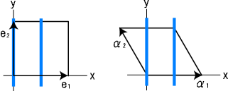
Figure 1: ${\mathbb{Z}}_{2}\times{\mathbb{Z}}_{2}$ orbifold. The left figure is factorizable orbifold, and the right one is non-factorizable one. Blue colored lines are fixed tori $T^{1}$.

This mechanism can be applied to higher dimensional Lie lattices, and generally the torus can not be factorized to $T^{2}\times T^{2}\times T^{2}$. We classify all ${\mathbb{Z}}_{N}\times{\mathbb{Z}}_{M}$ orbifold on SU($N$) and SO($N$) Lie lattice.

2.2 Supersymmetric condition

One can always choose diagonal basis for $\theta$ on SO(6):

$$\theta=\exp(2\pi i(aJ_{12}+bJ_{34}+cJ_{56})).$$ (10)

Then the eight eigenvalues of $\theta$ acting on the spinor of SO(8) are $e^{\pi i(\pm a+\pm b+\pm c)}$. To preserve ${\mathcal{N}}=1$ supersymmetry at least two of them should be left invariant. For convenience we list the thirteen shift vectors $(|a|,|b|,|c|)$ which are allowed by these conditions [2].

	$(|a|,|b|,|c|)$
$(0,\frac{1}{2},\frac{1}{2})$	$(0,\frac{1}{3},\frac{1}{3})$	$(\frac{1}{3},\frac{1}{3},\frac{2}{3})$	$(0,\frac{1}{4},\frac{1}{4})$	$(\frac{1}{4},\frac{1}{4},\frac{1}{2})$
$(0,\frac{1}{6},\frac{1}{6})$	$(\frac{1}{6},\frac{1}{6},\frac{1}{3})$	$(\frac{1}{6},\frac{1}{3},\frac{1}{2})$	$(\frac{1}{7},\frac{2}{7},\frac{3}{7})$	$(\frac{1}{8},\frac{1}{4},\frac{3}{8})$
$(\frac{1}{8},\frac{3}{8},\frac{1}{2})$	$(\frac{1}{12},\frac{1}{3},\frac{5}{12})$	$(\frac{1}{12},\frac{5}{12},\frac{1}{2})$

Table 1: The shift vectors of point group $\theta$, which satisfy the tachyon free condition.

In this paper ${\mathbb{Z}}_{2}\times{\mathbb{Z}}_{2}$, ${\mathbb{Z}}_{2}\times{\mathbb{Z}}_{3}$, ${\mathbb{Z}}_{2}\times{\mathbb{Z}}_{4}$ and ${\mathbb{Z}}_{4}\times{\mathbb{Z}}_{4}$ models are investigated. In following models, we can always select the shift vectors $v$ ($w$) of point group elements $\theta$ ($\phi$) of ${\mathbb{Z}}_{N}\times{\mathbb{Z}}_{M}$ as

$$\theta:~{}v = (n,-n,0)$$

$$\phi:~{}w = (0,m,-m)$$ (11)

where $n,m=\frac{1}{2}$ or $\frac{1}{3}$ or $\frac{1}{4}$. This projects out six components of the spinor, and leaves two chiral spinors $|\pm(\frac{1}{2},\frac{1}{2},\frac{1}{2},\frac{1}{2})\rangle$ invariant. Then ${\mathcal{N}}=1$ supersymmetry will be unbroken in four dimension.

A point group element of ${\mathbb{Z}}_{N}$ orbifold, which has no eigenvalues equal to 1 when acting on the six dimensional Lie lattice, is called non-degenerate. These elements which are generated by Weyl reflection on six dimensional Lie lattice, are classified by Carter diagram in ref.[13]. In Appendix.B we review Carter diagram and Coxeter elements shortly.

2.3 Modular invariance and discrete torsion

Heterotic orbifold models must satisfy some consistency conditions required by the modular invariance. The modular invariance guarantees the anomaly cancellation in low energy theory [9]. For $Z_{N}$ orbifolds with prime $N$, the level matching conditions are necessary and sufficient for modular invariance to all loops of string amplitude. For the $\theta^{k}\phi^{l}$-twisted sector, the level matching condition is

$$N^{\prime}[(kV+lW)^{2}-(kv+lw)^{2}]=0\bmod 2,$$ (12)

$$k=0,\cdots,N-1,~{}~{}l=0,\cdots,M-1,$$

where $N^{\prime}$ is the order of the twist $\theta^{k}\phi^{l}$, and $V$ and $W$ are the shift vectors in gauge sector associated to $\theta$ and $\phi$ respectively. In our paper we consider E${}_{8}\times$E${}_{8}^{\prime}$ heterotic string models with standard embedding. The shift vectors of gauge sector E₈ are given as

$$v=(n,-n,0)~{} \rightarrow V=(n,-n,0,0,0,0,0,0),$$ (13)

$$w=(0,m,-m)~{} \rightarrow W=(0,m,-m,0,0,0,0,0).$$

Thus the level matching condition is trivially satisfied in the standard embedding. This corresponds to embedding the spin connection in the gauge connection.

Turning on background antisymmetric field $B_{\mu\nu}$ on the torus it introduces phases to string state [9][10]. This effect can be described by the general form of one-loop partition function,

$$Z=\frac{1}{MN}\sum_{\theta,\phi}\epsilon(\theta,\phi)Z(\theta,\phi).$$ (14)

The phase $\epsilon(\theta,\phi)$ is called discrete torsion. In a ${\mathbb{Z}}_{N}$ orbifold these phase are fixed by one-loop modular invariance. On the other hand in ${\mathbb{Z}}_{N}\times{\mathbb{Z}}_{M}$ orbifolds, where $M$ is generally divisible by $N$, the phase is restricted to $N$-th root of unity,

$$\epsilon(\theta,\phi)\equiv\epsilon,~{}\epsilon^{N}=1.$$ (15)

Then the phases for general twisted sectors are given by

$$\epsilon(\theta^{k}\phi^{l},\theta^{t}\omega^{s})=\epsilon^{(ks-lt)}.$$ (16)

For orbifolds with non-prime $N$, we need to generalize the GSO projection [10]. The number of $\theta^{k}\phi^{l}$-twisted states is given by

$$D(\theta^{k}\phi^{l})=\frac{1}{MN}\sum_{t=0}^{N-1}\sum_{s=0}^{M-1}\epsilon^{(ks-lt)}\tilde{\chi}(\theta^{k}\phi^{l},\theta^{t}\omega^{s})\Delta(k,l;t,s),$$ (17)

where $\tilde{\chi}$ is the number of points left simultaneously fixed by $\theta^{k}\phi^{l}$ and $\theta^{t}\phi^{s}$. If $\theta^{k}\phi^{l}$ leaves unrotated some of the coordinates, $\tilde{\chi}$ must be calculated using only the sub-lattice which is rotated. $\Delta(k,l;t,s)$ is a state dependent phase. In the case of standard embedding it is given by

$$\Delta(k,l;t,s)=P^{(k,l)}\exp\{2\pi i[(p+kV+lW)(tV+sW)-(q+kv+lw)(tv+sw)]\},$$ (18)

where $P^{(k,l)}$ indicates a contribution of oscillators. $p$ is momentum of the E${}_{8}\times$E${}_{8}^{\prime}$ gauge sectors, and $q$ is H-momentum of the twisted states.

The generalization of the Euler characteristic of $Z_{N}$ orbifold is given by

$$\chi_{\epsilon}=\frac{1}{MN}\sum_{k,t=0}^{N-1}\sum_{l,s=0}^{M-1}\epsilon^{(ks-lt)}\chi(\theta^{k}\phi^{l},\theta^{t}\omega^{s}),$$ (19)

where $\chi$ is the number of points left simultaneously fixed by $\theta^{k}\phi^{l}$ and $\theta^{t}\phi^{s}$. The number of generations is equal to $\chi_{\epsilon}/2$. In section 4, we construct orbifold models for allowed values of $\epsilon$.

3 ${\mathbb{Z}}_{2}\times{\mathbb{Z}}_{2}$ orbifold: Factorisable VS non-factorizable

${\mathbb{Z}}_{2}\times{\mathbb{Z}}_{2}$ orbifold is phenomenologically interesting model, because some three generation models are presented with the aid of Wilson lines, and three generations may be associated to three complex dimension of compact space [4].

In heterotic orbifold model there are two classes of string states. One is untwisted sector in bulk and the other is twisted sector which localizes at fixed torus. The chirality of untwisted sector of ${\mathbb{Z}}_{2}\times{\mathbb{Z}}_{2}$ is left-right symmetric, so it does not contribute to the number of generations. The number of zero modes of twisted sector is related to the number of fixed tori. In a factorizable model with the action $\theta$ and $\phi$, whose shift vectors are $v=(\frac{1}{2},-\frac{1}{2},0)$ and $w=(0,\frac{1}{2},-\frac{1}{2})$ respectively, the number of tori of $\theta$-twisted sector is $4^{2}$, because there are four fixed points in the first and second tori, and the third torus is free from the action of $\theta$. Therefore the total number of zero modes of three twisted sectors is 48, and this corresponds to the generation numbers of ${\mathcal{N}}=1$ chiral matter which have gauge charge $27\in$ E₆ in the standard embedding.

We can confirm this result by calculating the Euler number, because the number of generations is equal to a half of Euler number [1],

$$\chi=\frac{1}{N}\sum_{[g,h]=0}\chi_{g,h},$$ (20)

where $\chi_{g,h}$ is the number of fixed points by action $g$ and $h$, and $N$ is the order of point group. For ${\mathbb{Z}}_{2}\times{\mathbb{Z}}_{2}$ orbifold, this equation is simplified to

$$\chi=\frac{3}{2}\chi_{\theta,\phi}.$$ (21)

Here, $\chi_{\theta,\phi}$ is the number of points left simultaneously fixed by $\theta$ and $\phi$, and is equal to $4^{3}$. Then we have $\chi=96$, and this agrees with the former result.

In the case of non-factorizable model it is easier to use Lefschetz fixed point theorem [7]. The number of fixed tori (#FT) of $\theta$-twisted sector is

$$\#FT={vol((1-\theta)\Lambda)\over vol(N)},$$ (22)

where $N$ is the lattice normal to the sub-lattice invariant by the action.

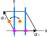
Figure 2: ${\mathbb{Z}}_{2}\times{\mathbb{Z}}_{2}$ orbifold. The blue colored lines are fixed tori by action of $\theta$. The circles and triangles are fixed points by action of $\phi$. The twisted states on the circles are mapped to the other by $\theta$, and the linear combinations of states are eigenstates of orbifold.

As an example we consider the orbifold model on SU(3)$\times$SO(8) root lattice, whose basis is given by simple roots,

$$\alpha_{1} = \sqrt{2}(1,0,0,0,0,0),$$

$$\alpha_{2} = \sqrt{2}\left(-\frac{1}{2},\frac{\sqrt{3}}{2},0,0,0,0\right),$$

$$\alpha_{3} = (0,0,1,-1,0,0),$$

$$\alpha_{4} = (0,0,0,1,-1,0),$$ (23)

$$\alpha_{5} = (0,0,0,0,1,-1),$$

$$\alpha_{6} = (0,0,0,0,1,1),$$

and ${\mathbb{Z}}_{2}\times{\mathbb{Z}}_{2}$ orbifold actions, $\theta$, $\phi$, are given by

$$\theta=\left(\begin{array}[]{cccccc}-1&0&0&0&0&0\\ 0&1&0&0&0&0\\ 0&0&1&0&0&0\\ 0&0&0&-1&0&0\\ 0&0&0&0&-1&0\\ 0&0&0&0&0&-1\end{array}\right),$$ (30)

$$\phi=\left(\begin{array}[]{cccccc}-1&0&0&0&0&0\\ 0&-1&0&0&0&0\\ 0&0&-1&0&0&0\\ 0&0&0&-1&0&0\\ 0&0&0&0&1&0\\ 0&0&0&0&0&1\end{array}\right).$$ (37)

The common fixed points by the actions of $\theta$ and $\phi$ are,

$$(0,0,0,0,0,0),~{}(0,0,1,0,0,0),~{}(0,0,0,0,\frac{1}{2},\pm\frac{1}{2}),$$

$$(\frac{\sqrt{2}}{2},0,0,0,0,0),~{}(\frac{\sqrt{2}}{2},0,1,0,0,0),~{}(\frac{\sqrt{2}}{2},0,0,0,\frac{1}{2},\pm\frac{1}{2}),$$

$$~{}(0,0,\frac{1}{2},\frac{1}{2},\underline{\pm\frac{1}{2},0}),~{}(\frac{\sqrt{2}}{2},0,\frac{1}{2},\frac{1}{2},\underline{\pm\frac{1}{2},0}),$$ (38)

where the underlined entries can be permuted. This leads to $\chi_{\theta,\phi}=16$ and $\chi=24$. Then the generation number is twelve. We can reconfirm this result by counting the number of fixed tori as follows. There are four independent fixed tori of the $\theta$-twisted sector,

$$(0,x,y,0,0,0),$$

$$(0,x,y,\underline{\frac{1}{2},\frac{1}{2},0}).$$ (39)

Note that these tori are identified by the sub lattice $(1-\theta)\Lambda$. The $\theta\phi$-twisted sector also has four fixed tori. In the $\phi$-twisted sector there are eight fixed tori,

$$(0,0,0,0,x,y),~{}(0,0,\frac{1}{2},\frac{1}{2},x,y),(\frac{\sqrt{2}}{2},0,0,0,x,y),~{}(\frac{\sqrt{2}}{2},0,\frac{1}{2},\frac{1}{2},x,y),$$

$$(\pm\frac{\sqrt{2}}{4},\frac{1}{2}\sqrt{\frac{3}{2}},0,0,x,y),~{}(\pm\frac{\sqrt{2}}{4},\frac{1}{2}\sqrt{\frac{3}{2}},\frac{1}{2},\frac{1}{2},x,y).$$ (40)

Then the total number of tori is 16, and does not match the generation number.

This is because two of fixed tori of the $\phi$-twisted sector are not invariant by the action of $\theta$. On the SU(3) torus in figure 2, there are four fixed points, and can be labeled by shift vector, $v=n\alpha_{1}+m\alpha_{2},~{}n,m=0,1$. The $\theta$-invariant states are

$$|0\rangle,~{}~{}|\alpha_{1}\rangle.$$ (41)

These are charged matter of representation $27$. We can take linear combination of remaining two states as eigenstates of action of $\theta$,

$$+1: ~{}|\alpha_{2}\rangle+|\alpha_{1}+\alpha_{2}\rangle,$$

$$-1: ~{}|\alpha_{2}\rangle-|\alpha_{1}+\alpha_{2}\rangle,$$ (42)

where $\pm 1$ denote the eigenvalue of these states under the action of $\theta$. The phase of physical states should be cancelled with $\Delta$-phase (18). These are the same chirality states with the charge of representation in $27$ and $\overline{27}$ respectively, and they do not contribute to the number of generations [7]. The generation number from the $\phi$-sector is four, and we have twelve generations from three twisted sectors, which is equal to a half of $\chi$. This is significantly small compared to the generation number of factorizable model.

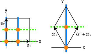
Figure 3: ${\mathbb{Z}}_{2}\times{\mathbb{Z}}_{2}$ orbifold. Blue colored lines are fixed tori by $\theta$ action, and green colored dotted lines are by $\theta\phi$ action. The circles are common fixed points.

The diminution of fixed tori and fixed points in SU(3) torus can be seen in figure 3. In this figure the basis of the SU(3) root lattice is changed to $\alpha_{1}+\alpha_{2}$ and $\alpha_{1}$, and that makes it easier to draw the orbifold action. In this figure we can see that the decrease of $\theta$ fixed tori of the non-factorizable model is related to direction which is left invariant by the action of $\theta$. Therefore the diminution does not occur in non-degenerate orbifold such as Coxeter orbifold which rotates the whole space of $T^{6}$.

4 ${\mathbb{Z}}_{N}\times{\mathbb{Z}}_{M}$ non-factorizable orbifold

As we have seen in ${\mathbb{Z}}_{2}\times{\mathbb{Z}}_{2}$ model, the number of fixed tori on non-factorizable orbifold is less than that of factorizable model due to the topological difference of fixed tori. The following shift vectors of point group elements which generate tori are

$$(0,\frac{1}{2},\frac{1}{2}),~{}(0,\frac{1}{3},\frac{1}{3}),~{}(0,\frac{1}{4},\frac{1}{4}),~{}(0,\frac{1}{6},\frac{1}{6}).$$ (43)

We call these elements degenerate. That means some eigenvalues of the point group element are equal to one. Then the model has ${\mathcal{N}}=2$ supersymmetry and non-chiral. In order for the resulting orbifold model to have ${\mathcal{N}}=1$ supersymmetry the point group of orbifold should be ${\mathbb{Z}}_{N}\times{\mathbb{Z}}_{M}$, and this is totally non-degenerate. We can embed some of these point group elements to non-factorizable tori.

Non-factorizable tori are defined by root lattices. Lie lattice of SO($2N$) are given by the simple roots,

$$\alpha_{1} = (1,-1,0,0,\cdots,0),$$

$$\alpha_{2} = (0,1,-1,0,\cdots,0),$$

$$\vdots$$

$$\alpha_{N-1} = (0,\cdots,0,1,-1),$$ (44)

$$\alpha_{N} = (0,\cdots,0,1,1),$$

and simple roots of SU($N$) are

$$\alpha_{1} = (1,-1,0,0,\cdots,0),$$

$$\alpha_{2} = (0,1,-1,0,\cdots,0),$$

$$\vdots$$

$$\alpha_{N-1} = (0,\cdots,1,-1,0),$$ (45)

$$\alpha_{N} = (0,\cdots,0,1,-1).$$

For simplicity we use the basis for SU(2) root lattice,

$$\alpha_{1}=(1).$$ (46)

Hereafter we use direct sum of these simple roots for the basis of compact space $T^{6}$.

4.1 ${\mathbb{Z}}_{2}\times{\mathbb{Z}}_{4}$ models

As an example we consider a model on SO(12) root lattice, which is the case that $N=6$ in (4). The only consistent point group action on this lattice, except its conjugate representation, is

$$\theta = \left(\begin{array}[]{ccccccc}0&-1&0&0&0&0\\ 1&0&0&0&0&0\\ 0&0&0&1&0&0\\ 0&0&-1&0&0&0\\ 0&0&0&0&1&0\\ 0&0&0&0&0&1\end{array}\right),$$ (53)

$$\phi = diag(1,1,-1,-1,-1,-1).$$

We count the number of states with representations $27$ and $\overline{27}$ by the use of the coordinates of fixed points and fixed tori . The $\theta^{i}\phi^{j}$-twisted sector $T_{ij}$ localizes at fixed points or tori as follows,

$$\begin{array}[]{ll}T_{01}:&(x,y,0,0,0,0),~{}(x,y,\underline{\frac{1}{2},\frac{1}{2},0,0}),~{}(x,y,\frac{1}{2},\frac{1}{2},\frac{1}{2},\frac{1}{2}),\\ T_{10}:&(0,0,x,y,0,0),~{}(\frac{1}{2},\frac{1}{2},x,y,\frac{1}{2},\frac{1}{2}),\\ T_{11}:&(0,0,0,0,0,0),~{}(1,0,0,0,0,0),~{}(\frac{1}{2},\frac{1}{2},0,0,\frac{1}{2},\pm\frac{1}{2}),\\ &(\frac{1}{2},\frac{1}{2},\underline{\pm\frac{1}{2},0},0,0),~{}(0,0,\underline{\frac{1}{2},0},\frac{1}{2},\pm\frac{1}{2}),\\ &(0,0,\frac{1}{2},\pm\frac{1}{2},0,0),~{}(\frac{1}{2},\frac{1}{2},\frac{1}{2},\frac{1}{2},\frac{1}{2},\pm\frac{1}{2}),\\ T_{20}:&(0,0,x,y,0,0),~{}(\frac{1}{2},\frac{1}{2},x,y,0,0),~{}(0,0,x,y,\frac{1}{2},\frac{1}{2})\\ &(\underline{\frac{1}{2},0},x,y,\underline{\frac{1}{2},0}),~{}(\frac{1}{2},\frac{1}{2},x,y,\frac{1}{2},\frac{1}{2}),\\ T_{21}:&(0,0,0,0,x,y),~{}(\underline{\frac{1}{2},\frac{1}{2},0,0},x,y),~{}(\frac{1}{2},\frac{1}{2},\frac{1}{2},\frac{1}{2},x,y).\end{array}$$ (62)

In the orbifolds of ${\mathbb{Z}}_{N}$ with non-prime $N$, the physical state of $\theta^{k}$-sector is generally linear combination of state at fixed points by the action $\theta^{k}$ [11, 6]. If $f_{k}$ is a fixed point of $\theta^{k}$ such that $l$ is the smallest number giving $\theta^{l}f_{k}=f_{k}+u,~{}u\in\Lambda$, then the eigenstates of $\theta$ are

$$|p\rangle=\sum_{r=0}^{n-1}e^{i\gamma r}|\theta^{r}f_{k}\rangle,$$ (63)

with $\gamma=2\pi/l$, $p=0,1,\cdots,N-1$. Then the physical states of $T_{01}$ sector by orbifold are linear combinations of them,

$$1: |(x,y,0,0,0,0)\rangle,~{}|(x,y,\frac{1}{2},\frac{1}{2},\frac{1}{2},\frac{1}{2})\rangle,$$

$$|(x,y,\frac{1}{2},\frac{1}{2},0,0)\rangle,~{}|(x,y,0,0,\frac{1}{2},\frac{1}{2})\rangle,$$

$$|(x,y,\frac{1}{2},0,\frac{1}{2},0)\rangle+|(x,y,0,\frac{1}{2},\frac{1}{2},0)\rangle,$$

$$|(x,y,\frac{1}{2},0,0,\frac{1}{2})\rangle+|(x,y,0,\frac{1}{2},0,\frac{1}{2})\rangle,$$

$$-1: |(x,y,\frac{1}{2},0,\frac{1}{2},0)\rangle-|(x,y,0,\frac{1}{2},\frac{1}{2},0)\rangle,$$

$$|(x,y,\frac{1}{2},0,0,\frac{1}{2})\rangle-|(x,y,0,\frac{1}{2},0,\frac{1}{2})\rangle,$$

where $\pm 1$ denote eigenvalues under the action of $\theta$. Then there are six states of $27\in E_{6}$, but the negative eigenvalue state does not make $\overline{27}$ state because it does not cancel the $\Delta$-phase (18). In this way we confirm the number of $27$ states is 34, and that of $\overline{27}$ states is 0. The untwisted sector is the same as factorizable model, that is $h^{1,1}_{untwisted}=3$ and $h^{2,1}_{untwisted}=1$. This is because the untwisted sector is determined by local action of orbifold and not affected by global structure of Lie lattice.

This result is confirmed by the Euler number (20),

$$\chi = \frac{1}{8}\left(24\chi_{\theta.\phi}+\chi_{1.\theta\phi}+\chi_{\theta^{2}.\phi}\right),$$

$$\chi_{-1} = \frac{1}{8}\left(-24\chi_{\theta.\phi}+\chi_{1.\theta\phi}+\chi_{\theta^{2}.\phi}\right).$$ (66)

Here, $\chi_{-1}/2$ is the generation number of the model with discrete torsion $\epsilon=-1$. The fixed points by the action of $\theta$ and $\phi$ are

$$(0,0,0,0,0,0),~{}(1,0,0,0,0,0),~{}(\frac{1}{2},\frac{1}{2},\frac{1}{2},\frac{1}{2},\frac{1}{2},\pm\frac{1}{2}),$$ (67)

$$(0,0,\frac{1}{2},\pm\frac{1}{2},0,0),~{}(\frac{1}{2},\frac{1}{2},0,0,\frac{1}{2},\pm\frac{1}{2}).$$

The fixed points of action of $\theta\phi$ are

$$(0,0,0,0,0,0),~{}(1,0,0,0,0,0),~{}(\frac{1}{2},\frac{1}{2},\frac{1}{2},\frac{1}{2},\frac{1}{2},\pm\frac{1}{2}),$$

$$(0,0,\frac{1}{2},\pm\frac{1}{2},0,0),~{}(\frac{1}{2},\frac{1}{2},0,0,\frac{1}{2},\pm\frac{1}{2}),$$ (68)

$$(\frac{1}{2},\frac{1}{2},\underline{\pm\frac{1}{2},0},0,0),~{}(0,0,\underline{\frac{1}{2},0},\frac{1}{2},\pm\frac{1}{2}).$$

The fixed points of action of $\theta^{2}$ and $\phi$ are

$$(0,0,0,0,0,0),~{}(1,0,0,0,0,0),~{}(\underline{\frac{1}{2},0},\underline{\frac{1}{2},0},\underline{\pm\frac{1}{2},0}),$$

$$(\frac{1}{2},\pm\frac{1}{2},0,0,0,0),~{}(0,0,\frac{1}{2},\pm\frac{1}{2},0,0),~{}(0,0,0,0,\frac{1}{2},\pm\frac{1}{2}),~{}$$ (69)

$$(\frac{1}{2},\frac{1}{2},\underline{\pm\frac{1}{2},0},0,0),~{}(0,0,\underline{\frac{1}{2},0},\frac{1}{2},\pm\frac{1}{2}),~{}(\frac{1}{2},\frac{1}{2},\frac{1}{2},\frac{1}{2},\frac{1}{2},\pm\frac{1}{2}).$$

As a result we have $\chi_{\theta.\phi}=8$, $\chi_{1.\theta\phi}=16$ and $\chi_{\theta^{2}.\phi}=32$. The generation numbers in these models are

$$\chi/2 = 36,$$

$$\chi_{-1}/2 = 12,$$ (70)

This result is different from that of factorizable tori SO(4)$\times$SO(4)$\times T^{2}$, i.e. $\chi/2=60$ and $\chi_{-1}/2=12$. All other models on non-factorizable tori are listed in Table 3 of Appendix.A.

4.2 ${\mathbb{Z}}_{4}\times{\mathbb{Z}}_{4}$ models

The basis of six dimensional tori SO(12) is given by (4). In SO(12) root lattice the only consistent point group action, except its conjugate representation, is

$$\theta = \left(\begin{array}[]{ccccccc}0&-1&0&0&0&0\\ 1&0&0&0&0&0\\ 0&0&0&1&0&0\\ 0&0&-1&0&0&0\\ 0&0&0&0&1&0\\ 0&0&0&0&0&1\end{array}\right),$$ (77)

$$\phi = \left(\begin{array}[]{ccccccc}1&0&0&0&0&0\\ 0&1&0&0&0&0\\ 0&0&0&-1&0&0\\ 0&0&1&0&0&0\\ 0&0&0&0&0&1\\ 0&0&0&0&-1&0\end{array}\right).$$ (84)

The $\theta^{i}\phi^{j}$-twisted sector $T_{ij}$ localizes at fixed points or tori as follows,

$$\begin{array}[]{ll}T_{01}:&(x,y,0,0,0,0),~{}(x,y,\frac{1}{2},\frac{1}{2},\frac{1}{2},\frac{1}{2}),\\ T_{02}:&(x,y,0,0,0,0),~{}(x,y,\underline{\frac{1}{2},\frac{1}{2},0,0}),~{}(x,y,\frac{1}{2},\frac{1}{2},\frac{1}{2},\frac{1}{2}),\\ T_{10}:&(0,0,0,0,x,y),~{}(\frac{1}{2},\frac{1}{2},\frac{1}{2},\frac{1}{2},x,y),\\ T_{11}:&(0,0,x,y,0,0),~{}(\frac{1}{2},\frac{1}{2},x,y,\frac{1}{2},\frac{1}{2}),\\ T_{12}:&(0,0,0,0,0,0),~{}(1,0,0,0,0,0),~{}(\frac{1}{2},\frac{1}{2},\frac{1}{2},\frac{1}{2},\frac{1}{2},\pm\frac{1}{2}),\\ &(\frac{1}{2},\frac{1}{2},\frac{1}{2},\pm\frac{1}{2},0,0),~{}(0,0,0,0,\frac{1}{2},\pm\frac{1}{2}),\\ &(\frac{1}{2},\frac{1}{2},0,0,\underline{\pm\frac{1}{2},0}),~{}(0,0,\frac{1}{2},\frac{1}{2},\underline{\pm\frac{1}{2},0}),\\ T_{13}:&(0,0,0,0,0,0),~{}(1,0,0,0,0,0),~{}(\frac{1}{2},\frac{1}{2},\frac{1}{2},\frac{1}{2},\frac{1}{2},\pm\frac{1}{2}),\\ &(0,0,\frac{1}{2},\pm\frac{1}{2},0,0),~{}(\frac{1}{2},\frac{1}{2},0,0,\frac{1}{2},\pm\frac{1}{2}),\\ &(\frac{1}{2},\frac{1}{2},\underline{\pm\frac{1}{2},0},0,0),~{}(0,0,\underline{\frac{1}{2},0},\frac{1}{2},\pm\frac{1}{2}),\\ T_{20}:&(0,0,0,0,x,y),~{}(\underline{\frac{1}{2},\frac{1}{2},0,0},x,y),~{}(\frac{1}{2},\frac{1}{2},\frac{1}{2},\frac{1}{2},x,y),\\ T_{22}:&(0,0,x,y,0,0),~{}(\underline{\frac{1}{2},\frac{1}{2}},x,y,\underline{0,0}),~{}(\frac{1}{2},\frac{1}{2},x,y,\frac{1}{2},\frac{1}{2}),\\ T_{23}:&(0,0,0,0,0,0),~{}(1,0,0,0,0,0),~{}(\frac{1}{2},\frac{1}{2},\frac{1}{2},\frac{1}{2},\frac{1}{2},\pm\frac{1}{2}),\\ &(0,0,\frac{1}{2},\frac{1}{2},\frac{1}{2},\pm\frac{1}{2}),~{}(\frac{1}{2},\pm\frac{1}{2},0,0,0,0),\\ &(\underline{\frac{1}{2},0},\frac{1}{2},\pm\frac{1}{2},0,0),~{}(\underline{\frac{1}{2},0},0,0,\frac{1}{2},\pm\frac{1}{2}).\end{array}$$ (100)

There are 51 orbifold invariant states, $h^{1,1}_{twisted}=51$ and $h^{2,1}_{twisted}=0$. The untwisted sector is the same as factorizable model, that is $h^{1,1}_{untwisted}=3$ and $h^{2,1}_{untwisted}=0$.

This result is confirmed by the Euler number (20),

$$\chi = \frac{1}{16}\{96\chi_{\theta.\phi}+24(\chi_{\theta^{2}.\phi}+\chi_{\theta.\phi^{2}}+\chi_{\theta\phi,\phi^{2}})$$

$$+12(\chi_{1.\theta\phi^{2}}+\chi_{1.\theta\phi^{3}}+\chi_{1.\theta^{2}\phi})+6\chi_{\theta^{2}.\phi^{2}}\},$$

$$\chi_{-1} = \frac{1}{16}\{-96\chi_{\theta.\phi}+24(\chi_{\theta^{2}.\phi}+\chi_{\theta.\phi^{2}}+\chi_{\theta\phi,\phi^{2}})$$ (101)

$$+12(\chi_{1.\theta\phi^{2}}+\chi_{1.\theta\phi^{3}}+\chi_{1.\theta^{2}\phi})+6\chi_{\theta^{2}.\phi^{2}}\},$$

$$\chi_{\pm i} = \frac{1}{16}\{-24(\chi_{\theta^{2}.\phi}+\chi_{\theta.\phi^{2}}+\chi_{\theta\phi,\phi^{2}})$$

$$+12(\chi_{1.\theta\phi^{2}}+\chi_{1.\theta\phi^{3}}+\chi_{1.\theta^{2}\phi})+6\chi_{\theta^{2}.\phi^{2}}\}.$$

Here, $\chi_{-1}/2$ and $\chi_{\pm i}/2$ are equal to generation numbers of the models with discrete torsion $\epsilon=-1$ and $\epsilon=\pm i$ respectively. We can calculate these quantities in a similar manner with the former section, and the result is

$$\chi_{\theta.\phi}=4,~{}\chi_{1.\theta\phi}=16,~{}\chi_{\theta^{2}.\phi}=8,~{}\chi_{\theta^{2}.\phi^{2}}=32,$$ (102)

and the generation numbers in these models are obtained as

$$\chi/2 = 54,$$

$$\chi_{-1}/2 = 30,$$

$$\chi_{\pm i}/2 = 6,$$ (103)

This result is different from that of factorizable tori SO(4)$\times$SO(4)$\times$SO(4), i.e. $\chi/2=90$, $\chi_{-1}/2=42$ and $\chi_{\pm i}/2=-6$.

In the ${\mathbb{Z}}_{4}\times{\mathbb{Z}}_{4}$ orbifold, only three lattices are allowed, and the last one is SO(8)$\times$SO(4). The basis of six dimensional tori SO(8)$\times$SO(4) are given by

$$\alpha_{1} = (1,-1,0,0,0,0),$$

$$\alpha_{2} = (0,1,-1,0,0,0),$$

$$\alpha_{3} = (0,0,1,-1,0,0),$$

$$\alpha_{4} = (0,0,1,1,0,0),$$ (104)

$$\alpha_{5} = (0,0,0,0,1,-1),$$

$$\alpha_{6} = (0,0,0,0,1,1).$$

The point group actions are the same as that of (84). However the number of fixed tori is different from that of SO(12) lattice. The numbers of fixed points are

$$\chi_{\theta.\phi}=4,~{}\chi_{1.\theta\phi}=16,~{}\chi_{\theta^{2}.\phi}=8,~{}\chi_{\theta^{2}.\phi^{2}}=32,$$ (105)

and the generation numbers of these models are obtained as

$$\chi/2 = 60,$$

$$\chi_{-1}/2 = 36,$$

$$\chi_{\pm i}/2 = 0.$$ (106)

These are all models which are allowed in the ${\mathbb{Z}}_{4}\times{\mathbb{Z}}_{4}$ orbifold on Lie lattices.

4.3 ${\mathbb{Z}}_{2}\times{\mathbb{Z}}_{3}$ models

The point group elements $\theta$, $\phi$ of ${\mathbb{Z}}_{2}\times{\mathbb{Z}}_{3}$ orbifold can be expressed by one element $\theta\phi\in{\mathbb{Z}}_{6}$ which is non-degenerate. Let $\omega$ be defined by $\omega\equiv\theta\phi$. Then we have $\theta=\omega^{4}$ and $\phi=\omega^{3}$. This implies ${\mathbb{Z}}_{2}\times{\mathbb{Z}}_{3}$ orbifold is essentially non-degenerate and does not provide new models which have different Euler number compared to factorizable model. The Euler characteristic of ${\mathbb{Z}}_{2}\times{\mathbb{Z}}_{3}$ orbifold is evaluated by (20), and it is simplified to

$$\chi=4\chi_{1.\omega}.\\$$ (107)

We see that only non-degenerate element $\omega\in{\mathbb{Z}}_{6}$ contributes to the generation numbers of these models. However the Hodge numbers are dependent on lattices as we see below.

For example the basis of six dimensional tori SO(6)$\times$SU(3)$\times$SU(2) is given by

$$\alpha_{1} = (1,-1,0,0,0,0,0),$$

$$\alpha_{2} = (0,1,-1,0,0,0,0),$$

$$\alpha_{3} = (0,1,1,0,0,0,0),$$

$$\alpha_{4} = (0,0,0,1,-1,0,0),$$ (108)

$$\alpha_{5} = (0,0,0,0,1,-1,0),$$

$$\alpha_{6} = (0,0,0,0,0,0,1).$$

In the SO(6)$\times$SU(3)$\times$SU(2) root lattice the only consistent point group action, except its conjugate, is

$$\theta = \left(\begin{array}[]{ccccccc}0&1&0&0&0&0&0\\ 0&0&1&0&0&0&0\\ 1&0&0&0&0&0&0\\ 0&0&0&0&1&0&0\\ 0&0&0&0&0&1&0\\ 0&0&0&1&0&0&0\\ 0&0&0&0&0&0&1\end{array}\right),$$ (116)

$$\phi = diag(-1,-1,-1,1,1,1,-1).$$

In SO(6) root lattice subspace there is only one fixed tori, which is depicted as figure 4.

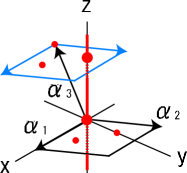
Figure 4: ${\mathbb{Z}}_{2}\times{\mathbb{Z}}_{3}$ non-factorizable orbifold. Circles are points on the $\theta$ fixed tori which are parallel to z-axis. Red colored line on z-axis is a fixed tori by $\theta$ action, and we can see two circles are on the line. Due to lattice structure all circles are on the same fixed torus. So there is only one fixed torus in $\theta$-twisted sector.

The Hodge numbers are calculated as $h^{1,1}_{twisted}=26$ and $h^{2,1}_{twisted}=4$ from the $\omega^{i}$-twisted sector $T_{i}$ localizing at fixed points or tori. The untwisted sector is the same as factorizable model, that is $h^{1,1}_{untwisted}=3$ and $h^{2,1}_{untwisted}=1$. As we have mentioned the number of generations is 24, which is the same as the factorizable model. However this model has different Hodge numbers from that of the factorizable model on SU(3)³ root lattice.

Similarly the other two ${\mathbb{Z}}_{2}\times{\mathbb{Z}}_{3}$ models are examined, and the results are listed in Appendix A. The non-factorizable models are not same orbifolds as factorizable one and the structure of Yukawa coupling can be different from the factorizable model.

5 Conclusion and discussion

In this paper we have generalized ${\mathbb{Z}}_{2}\times{\mathbb{Z}}_{2}$ non-factorizable orbifold [7] to ${\mathbb{Z}}_{N}\times{\mathbb{Z}}_{M}$, and show that it provides new classes of abelian orbifolds. In Appendix A, we give fairly complete classification of non-factorizable abelian orbifolds on SO($N$) and SU($N$) root lattices. The generation numbers of the models $\chi_{\epsilon}/2$ are always multiples of 12. As we have explained in sections 3 and 4, the Euler numbers of non-factorizable orbifolds are smaller than that of factorizable models. This will be favorable for phenomenological motivation to have three generation matter. Moreover the Yukawa coupling can be changed in non-factorizable models [8], and there is a possibility to realize the quark and lepton mass matrix with appropriate mixing.

To construct realistic orbifold heterotic string, introducing Wilson lines will be important. It is interesting to look for realistic models using the techniques introduced in this paper. There may be correspondence between ${\mathbb{Z}}_{N}\times{\mathbb{Z}}_{M}$ non-factorizable orbifolds and the free fermionic models of heterotic string. We see that there are wide classes of ${\mathbb{Z}}_{N}\times{\mathbb{Z}}_{M}$ orbifolds, and they are interesting in their own right.

Acknowledgement

I would like to thank T.Kobayashi for valuable discussions and advice, and M.Hanada, and the other members of particle physics group of Kyoto University. I am grateful to P.Vaudrevange and S.Ramos-Sanchez for pointing out some errors on the tables, and interesting coincidence [14]. K. T. is supported by the Grand-in-Aid for Scientific Research #172131.

Appendix A Non-factorizable orbifold models

In this appendix we list the all non-factorizable models, especially the compactified Lie lattices and their generation numbers. All results of our paper are listed here. We observe the generation numbers of the models $\chi_{\epsilon}/2$ are always multiples of 12.

General remark is as follows. If we give the Lie lattice for ${\mathbb{Z}}_{N}\times{\mathbb{Z}}_{M}$ orbifold, the point group elements are uniquely determined up to their conjugate representations. Therefore we classify ${\mathbb{Z}}_{N}\times{\mathbb{Z}}_{M}$ orbifolds by their Lie lattices. As we include Weyl group and graph automorphisms to the point groups, SU(3) and G₂ root lattices are equivalent, and the same for SO(8) and F₄ root lattices, SO($2N$) and SO($2N+1$) root lattices respectively.

We also calculate the generation numbers $\chi/2$ by

$$\frac{\chi}{2}=h^{1,1}_{untwisted}-h^{2,1}_{untwisted}+h^{1,1}_{twisted}-h^{2,1}_{twisted},$$ (117)

where $h^{1,1}_{twisted}$ and $h^{2,1}_{twisted}$ are the numbers of chiral matter fields from twisted sectors with representation in $27$ and $\overline{27}$ respectively. Similarly $h^{1,1}_{untwisted}$ and $h^{2,1}_{untwisted}$ are that of untwisted sectors, and they are independent of Lattice structure.

A.1 ${\mathbb{Z}}_{2}\times{\mathbb{Z}}_{2}$

The result of ${\mathbb{Z}}_{2}\times{\mathbb{Z}}_{2}$ orbifold models are examined in ref [7, 8]. The Euler number is simplified as

$$\chi=\frac{3}{2}\chi_{\theta,\phi}.$$ (118)

The allowed values of discrete torsion are

$$\epsilon=\pm 1.$$ (119)

However these discrete torsions do not make difference of generation numbers, except its sign. For all models, the numbers of zero modes of untwisted sector are

$$h^{1,1}_{untwisted}=h^{2,1}_{untwisted}=3.$$ (120)

The Hodge number of twisted sectors and the generation numbers of ${\mathbb{Z}}_{2}\times{\mathbb{Z}}_{2}$ orbifold models are listed in table 2. The factorizable model is expressed as $T^{2}\times T^{2}\times T^{2}$, because the complex structure of each torus is not fixed by orbifold action.

Lattice	$\epsilon$	$\chi$	$h^{1,1}_{twisted}$	$h^{2,1}_{twisted}$
$T^{2}\times T^{2}\times T^{2}$	1	96	48	0
	-1	-96	0	48
SU(3)$\times$SU(2)4	1	48	28	4
	-1	-48	4	28
SU(4)$\times$SU(2)3	1	48	24	0
	-1	-48	0	24
SU(3)${}^{2}\times$SU(2)${}^{2}-I$	1	24	18	6
	-1	-24	6	18
SU(3)${}^{2}\times$SU(2)${}^{2}-II$	1	24	16	4
	-1	-24	4	16
SU(4)$\times$SU(3)$\times$SU(2)	1	24	14	2
	-1	-24	2	14
SU(4)2	1	24	12	0
	-1	-24	0	12
SU(3)3	1	12	9	3
	-1	-12	3	9

Table 2: ${\mathbb{Z}}_{2}\times{\mathbb{Z}}_{2}$ orbifold models for standard embedding: The second column denotes values of the discrete torsion $\epsilon$. The generation numbers are given by $\chi/2$.

A.2 ${\mathbb{Z}}_{2}\times{\mathbb{Z}}_{4}$

The Euler number and the number of generations with the discrete torsion are

$$\chi = \frac{1}{8}\left(24\chi_{\theta.\phi}+\chi_{1.\theta\phi}+\chi_{\theta^{2}.\phi}\right),$$

$$\chi_{-1} = \frac{1}{8}\left(-24\chi_{\theta.\phi}+\chi_{1.\theta\phi}+\chi_{\theta^{2}.\phi}\right).$$ (121)

The allowed values of discrete torsion are

$$\epsilon=\pm 1.$$ (122)

For all models, the number of zero modes of untwisted sector are

$$h^{1,1}_{untwisted}=3,~{}h^{2,1}_{untwisted}=1.$$ (123)

The ${\mathbb{Z}}_{2}\times{\mathbb{Z}}_{4}$ orbifold models are listed in table 3. The factorizable model is expressed as SO(4)$\times$SO(4)$\times T^{2}$.

Lattice	$\epsilon$	$\chi$	$h^{1,1}_{twisted}$	$h^{2,1}_{twisted}$
SO(4)$\times$SO(4)$\times T^{2}$	1	120	58	0
	-1	24	18	8
SO(6)2	1	48	24	2
	-1	24	14	4
SO(6)$\times$SO(4)$\times$SU(2)	1	72	36	2
	-1	24	16	6
SO(8)$\times T^{2}$	1	96	48	2
	-1	0	8	10
SO(8)$\times$SO(4)	1	72	36	2
	-1	24	16	6
SO(10)$\times$SU(2)	1	72	34	0
	-1	24	14	4
SO(12)	1	72	34	0
	-1	24	14	4

Table 3: ${\mathbb{Z}}_{2}\times{\mathbb{Z}}_{4}$ orbifold models for standard embedding.

A.3 ${\mathbb{Z}}_{4}\times{\mathbb{Z}}_{4}$

The Euler number and the numbers of generations with the discrete torsions are

$$\chi = \frac{1}{16}\{96\chi_{\theta.\phi}+24(\chi_{\theta^{2}.\phi}+\chi_{\theta.\phi^{2}}+\chi_{\theta\phi,\phi^{2}})$$

$$+12(\chi_{1.\theta\phi^{2}}+\chi_{1.\theta\phi^{3}}+\chi_{1.\theta^{2}\phi})+6\chi_{\theta^{2}.\phi^{2}}\},$$

$$\chi_{-1} = \frac{1}{16}\{-96\chi_{\theta.\phi}+24(\chi_{\theta^{2}.\phi}+\chi_{\theta.\phi^{2}}+\chi_{\theta\phi,\phi^{2}})$$ (124)

$$+12(\chi_{1.\theta\phi^{2}}+\chi_{1.\theta\phi^{3}}+\chi_{1.\theta^{2}\phi})+6\chi_{\theta^{2}.\phi^{2}}\},$$

$$\chi_{\pm i} = \frac{1}{16}\{-24(\chi_{\theta^{2}.\phi}+\chi_{\theta.\phi^{2}}+\chi_{\theta\phi,\phi^{2}})$$

$$+12(\chi_{1.\theta\phi^{2}}+\chi_{1.\theta\phi^{3}}+\chi_{1.\theta^{2}\phi})+6\chi_{\theta^{2}.\phi^{2}}\}.$$

The allowed values of discrete torsion are

$$\epsilon=\pm 1,~{}\pm i.$$ (125)

For all models, the numbers of zero modes of untwisted sector are

$$h^{1,1}_{untwisted}=3,~{}h^{2,1}_{untwisted}=0.$$ (126)

The ${\mathbb{Z}}_{4}\times{\mathbb{Z}}_{4}$ orbifold models are listed in table 4. The factorizable model is expressed as SO(4)$\times$SO(4)$\times$SO(4).

Lattice	$\epsilon$	$\chi$	$h^{1,1}_{twisted}$	$h^{2,1}_{twisted}$
SO(4)$\times$SO(4)$\times$SO(4)	1	180	87	0
	-1	84	39	0
	$\pm i$	-12	3	12
SO(8)$\times$SO(4)	1	120	58	1
	-1	72	34	1
	$\pm i$	0	6	9
SO(12)	1	108	51	0
	-1	60	27	0
	$\pm i$	12	9	6

Table 4: ${\mathbb{Z}}_{4}\times{\mathbb{Z}}_{4}$ orbifold models for standard embedding.

A.4 ${\mathbb{Z}}_{2}\times{\mathbb{Z}}_{3}$

The Euler number is simplified as

$$\chi=4\chi_{1.\omega},\\$$ (127)

The discrete torsion is trivial in this case, i.e.

$$\epsilon=1.$$ (128)

For all models, the numbers of zero modes of untwisted sector are

$$h^{1,1}_{untwisted}=3,~{}h^{2,1}_{untwisted}=1.$$ (129)

The ${\mathbb{Z}}_{2}\times{\mathbb{Z}}_{3}$ orbifold models are listed in table 5. As we mentioned before, we do not distinguish SU(3) root lattice from $G_{2}$ root lattice, then the factorizable model can be expressed as SU(3)³.

Lattice	$\epsilon$	$\chi$	$h^{1,1}_{twisted}$	$h^{2,1}_{twisted}$
SU(3)3	1	48	32	10
SO(6)$\times$SU(3)$\times$SU(2)	1	48	26	4
SO(8)$\times$SU(3)	1	48	26	4
SU(5)$\times$SU(3)	1	48	26	4

Table 5: ${\mathbb{Z}}_{2}\times{\mathbb{Z}}_{3}$ orbifold models for standard embedding.

The numbers of $h^{1,1}_{twisted}$ and $h^{2,1}_{twisted}$ are same in non-factorizable models. This implies they are in equivalent class of orbifolds, and connected by continuous deformation of geometric moduli.

Appendix B Lie lattice and Weyl group

The basics of Weyl reflection, Coxeter elements and their explicit representations are given in this appendix. The point groups considered so far [6, 11, 12] are generated by Coxeter elements from Cater diagrams or generalized Coxeter elements which include graph automorphisms. We give explicit representations of point group elements generated by Weyl reflections and graph automorphisms of Lie lattices. Besides the generalized Coxeter elements this point group contains non-Coxeter elements. We utilize these elements for point group of our orbifold models.

B.1 Weyl reflection and graph automorphism

The Weyl group ${\mathcal{W}}$ is generated by the following Weyl reflections

$$r_{\alpha_{k}}:\lambda\rightarrow\lambda-2{\alpha_{k}\cdot\lambda\over\alpha_{k}\cdot\alpha_{k}}\alpha_{k},$$ (130)

where $\alpha_{k}$ is a simple root of the Lie lattice.

Convenient basis for simple root of SO($2N$) lattice can be set by $N$ elements vectors,

$$\alpha_{1} = (1,-1,0,0,\cdots,0),$$

$$\alpha_{2} = (0,1,-1,0,\cdots,0),$$

$$\vdots$$

$$\alpha_{N-1} = (0,\cdots,0,1,-1),$$ (131)

$$\alpha_{N} = (0,\cdots,0,1,1).$$

Then the Weyl reflections of these roots are represented by $N\times N$ matrices,

$$r_{\alpha_{n}}=\bordermatrix{&&&&n&n+1&&\cr&1&0&\cdots&0&0&\cdots&0\cr&0&1&\cdots&0&0&\cdots&0\cr&\vdots&\vdots&&\vdots&\vdots&&\vdots\cr&0&0&\cdots&0&1&\cdots&0\cr&0&0&\cdots&1&0&\cdots&0\cr&\vdots&\vdots&&\vdots&\vdots&&\vdots\cr&0&0&\cdots&0&0&\cdots&1}\begin{array}[]{ l }\\ \\ \\ n\\ n+1\\ \\ \\ \end{array},$$ (132)

for $n=1,\cdots,N-1$, and

$$r_{\alpha_{N}}=\left(\begin{array}[]{ c c c c c c}1&0&\cdots&0&0&0\\ 0&1&\cdots&0&0&0\\ \vdots&\vdots&&\vdots&\vdots&\vdots\\ 0&0&\cdots&1&0&0\\ 0&0&\cdots&0&0&-1\\ 0&0&\cdots&0&-1&0\end{array}\right).$$ (133)

The graph automorphism $g$ of Cartan diagram is represented as

$$g=\left(\begin{array}[]{ c c c c c}1&0&\cdots&0&0\\ 0&1&\cdots&0&0\\ \vdots&\vdots&&\vdots&\vdots\\ 0&0&\cdots&1&0\\ 0&0&\cdots&0&-1\end{array}\right).$$ (134)

One can easily find that $r_{\alpha_{n}}$ for $n=1,\cdots,N-1$ generate permutation group $S_{N}$. For example, the product of two Weyl reflections which do not commute each other makes up ${\mathbb{Z}}_{3}$ element, and the group is $S_{3}$. Moreover if we add the graph automorphism $g\in G_{out}$ to Weyl group, we can change the sign of any matrix elements of $S_{N}$. Then the orders of group ${\mathcal{W}}$ and $\{{\mathcal{W}},G_{out}\}$ are evaluated as table 6.

For SU($N-1$), we take the basis of $N$ elements, $\alpha_{n}$, $n=1,\cdots,N-1$, and graph automorphism is given by the following $N\times N$ matrix,

$$g=\left(\begin{array}[]{ c c c c c}0&0&\cdots&0&-1\\ 0&0&\cdots&-1&0\\ \vdots&\vdots&&\vdots&\vdots\\ 0&-1&\cdots&0&0\\ -1&0&\cdots&0&0\end{array}\right).$$ (135)

We can always diagonalize $g$ by the elements of ${\mathcal{W}}$, and this is negative of identity matrix, $-1\!\!1_{N}\equiv diag(-1,-1,\cdots,-1)$, this means $\{{\mathcal{W}},G_{out}\}=\{{\mathcal{W}},-1\!\!1_{N}\}$. Therefore the order of $\{{\mathcal{W}},G_{out}\}$ is twice as that of ${\mathcal{W}}$, as in table 6.

	${\mathcal{W}}$	$\{{\mathcal{W}},G_{out}\}$
SO($2N$)	$2^{N-1}N!$	$2^{N}N!$
SU($N$)	$N!$	$2N!$

Table 6: The order of Weyl group and graph automorphism

B.2 Coxeter element

The Coxeter element of the Lie lattice is defined by product of all simple roots,

$$D_{n}\equiv r_{\alpha_{1}}r_{\alpha_{2}}\cdots r_{\alpha_{N}}.$$ (136)

The other Coxeter elements, which are generated by different ordering of product, are conjugate to one another, and lead to the same class of orbifold.

In general there are other non-degenerate elements generated by Weyl reflections. These non-degenerate orbifold can be classified by the Carter diagrams [13]. The Coxeter elements of SO(8) from Carter diagrams are

$$D_{4} = r_{\alpha_{1}}r_{\alpha_{2}}r_{\alpha_{3}}r_{\alpha_{4}}=\left(\begin{array}[]{cccc}0&0&-1&0\\ 1&0&0&0\\ 0&1&0&0\\ 0&0&0&-1\end{array}\right),~{}$$ (141)

$$D_{4}(a1) = r_{\alpha_{1}}r_{\alpha_{2}}r_{\alpha_{3}}r_{\alpha_{2}+\alpha_{3}+\alpha_{4}}=\left(\begin{array}[]{cccc}0&-1&0&0\\ 1&0&0&0\\ 0&0&0&1\\ 0&0&-1&0\end{array}\right),~{}$$ (146)

where $r_{\alpha_{2}+\alpha_{3}+\alpha_{4}}$ is a Weyl reflection of the root generated by the sum of simple roots $\alpha_{2}+\alpha_{3}+\alpha_{4}$. Then the order of $D_{4}$ is six, and that of $D_{4}(a1)$ is four.

Figure 5: Carter diagrams

If we add the graph automorphism of Dynkin diagram to Weyl group, we can define generalized Coxeter elements. For example the SO($2N$) Lie lattice has graph automorphism $g\in G_{out}$ which exchanges the simple root $\alpha_{N-1}$ and $\alpha_{N}$, then we can define the generalized Coxeter element,

$$C^{[2]}\equiv r_{\alpha_{1}}r_{\alpha_{2}}\cdots r_{\alpha_{N-2}}g.$$ (147)

The generalized Coxeter element of SO(8) are

$$C^{[2]}=r_{\alpha_{1}}r_{\alpha_{2}}r_{\alpha_{3}}g=\left(\begin{array}[]{cccc}0&0&0&-1\\ 1&0&0&0\\ 0&1&0&0\\ 0&0&1&0\end{array}\right).$$ (148)

The order of this element is eight.

In the case of SO(8) lattice there is another graph automorphism $g^{\prime}\in G_{out}$, which permutes $\alpha_{1}\rightarrow\alpha_{3}\rightarrow\alpha_{4}$ cyclically. The generalized Coxeter element of this graph automorphism is

$$C^{[3]}\equiv r_{\alpha_{1}}r_{\alpha_{2}}g^{\prime}=\left(\begin{array}[]{cccc}\frac{1}{2}&\frac{-1}{2}&\frac{1}{2}&\frac{1}{2}\\ \frac{1}{2}&\frac{1}{2}&\frac{1}{2}&\frac{-1}{2}\\ \frac{1}{2}&\frac{1}{2}&\frac{-1}{2}&\frac{1}{2}\\ \frac{1}{2}&\frac{-1}{2}&\frac{-1}{2}&\frac{-1}{2}\end{array}\right).$$ (149)

However this graph automorphism does not provide new orbifold in the non-factorizable models.

B.3 General point group element on Lie lattice

In the case of ${\mathbb{Z}}_{N}\times{\mathbb{Z}}_{M}$ orbifolds there are other ${\mathcal{N}}=1$ supersymmetric models which are not generated by Coxeter elements, because one element of point group can be degenerate.

We can explicitly see all ${\mathbb{Z}}_{2}$ elements of SO($N$) lattice are

$$\theta_{{\mathbb{Z}}_{2}}=\left(\begin{array}[]{ c c c c c c c c c}0&1&&&&&&\cdots&0\\ 1&0&&&&&&&\vdots\\ &&\ddots&&&&&&\\ &&&0&-1&&&&\\ &&&-1&0&&&&\\ &&&&&\ddots&&&\\ &&&&&&-1&&\\ \vdots&&&&&&&\ddots&\\ 0&\cdots&&&&&&&1\end{array}\right),$$ (150)

and its permutations of Cartesian coordinates. The ${\mathbb{Z}}_{N}$ elements are constructed similarly. For example ${\mathbb{Z}}_{3}$ elements are constructed by the following sub-matrices,

$$\left(\begin{array}[]{ccc}0&0&1\\ 1&0&0\\ 0&1&0\end{array}\right),~{}\left(\begin{array}[]{ccc}0&0&1\\ -1&0&0\\ 0&-1&0\end{array}\right).$$ (151)

and their permutations. ${\mathbb{Z}}_{4}$ elements includes the following sub-matrices,

$$\left(\begin{array}[]{cccc}0&0&0&1\\ 1&0&0&0\\ 0&1&0&0\\ 0&0&1&0\end{array}\right),~{}\left(\begin{array}[]{cccc}0&0&0&1\\ -1&0&0&0\\ 0&-1&0&0\\ 0&0&1&0\end{array}\right),~{}\left(\begin{array}[]{cccc}0&0&0&-1\\ -1&0&0&0\\ 0&-1&0&0\\ 0&0&-1&0\end{array}\right),~{}\left(\begin{array}[]{cc}0&-1\\ 1&0\end{array}\right),$$ (152)

and their permutations.

In this way we can construct Coxeter and generalized Coxeter elements of Weyl group easily and intuitively. Similarly all point group elements we use in this paper can be expressed by Weyl reflections and the graph automorphism.

References

• [1] L. J. Dixon, J. A. Harvey, C. Vafa and E. Witten, Nucl. Phys. B 261 (1985) 678.
• [2] L. J. Dixon, J. A. Harvey, C. Vafa and E. Witten, Nucl. Phys. B 274 (1986) 285.
• [3] T. Kobayashi, S. Raby and R. J. Zhang, Phys. Lett. B 593, 262 (2004) [arXiv:hep-ph/0403065]; Nucl. Phys. B 704, 3 (2005) [arXiv:hep-ph/0409098].
• [4] S. Förste, H. P. Nilles, P. K. S. Vaudrevange and A. Wingerter, Phys. Rev. D 70, 106008 (2004);
• [5] S. Förste, H. P. Nilles and A. Wingerter, Phys. Rev. D 72, 026001 (2005) [arXiv:hep-th/0504117]; Phys. Rev. D 73, 066011 (2006) [arXiv:hep-th/0512270]. W. Buchmüller, K. Hamaguchi, O. Lebedev and M. Ratz, Nucl. Phys. B 712, 139 (2005) [arXiv:hep-ph/0412318]; Phys. Rev. Lett.  96, 121602 (2006) [arXiv:hep-ph/0511035]; arXiv:hep-th/0606187; H. P. Nilles, S. Ramos-Sanchez, P. K. S. Vaudrevange and A. Wingerter, JHEP 0604, 050 (2006) [arXiv:hep-th/0603086];
• [6] D. Bailin and A. Love, Phys. Rept.  315 (1999) 285.
• [7] A. E. Faraggi, S. Forste and C. Timirgaziu, JHEP 0608 (2006) 057 [arXiv:hep-th/0605117].
• [8] S. Forste, T. Kobayashi, H. Ohki and K. j. Takahashi, arXiv:hep-th/0612044.
• [9] C. Vafa, Nucl. Phys. B 273 (1986) 592.
• [10] A. Font, L. E. Ibanez and F. Quevedo, Phys. Lett. B 217 (1989) 272.
• [11] T. Kobayashi and N. Ohtsubo, Phys. Lett. B 262 (1991) 425.
• [12] T. Kobayashi and N. Ohtsubo, Int. J. Mod. Phys. A 9 (1994) 87.
• [13] A. N. Schellekens and N. P. Warner, Nucl. Phys. B 308 (1988) 397.
• [14] F. Ploger, S. Ramos-Sanchez, M. Ratz and P. K. S. Vaudrevange, arXiv:hep-th/0702176.