HD-THEP-07-4

Yang-Mills thermodynamics at low temperature

Ralf Hofmann

Institut für Theoretische Physik

Universität Heidelberg

Philosophenweg 16

69120 Heidelberg, Germany

For the confining phase of SU(2) Yang-Mills thermodynamics we show that the asymptotic series representing the pressure is Borel summable for negative (unphysical) values of a suitably defined coupling constant. The inverse Borel transform is meromorphic except for a branch cut along the positive-real axis. The physical pressure is precisely nil at vanishing and acquires a small imaginary admixture at small temperature the latter indicating violations of thermal equilibrium (turbulences).

1 Introduction and miniature review

To understand the (thermo-)dynamics of strongly coupled Yang-Mills theories is of importance both in view of an unearthing of their interesting mathematical structures and an exploitation of these theories in physical applications.

As discussed in [1, 2], SU(2) and SU(3) Yang-Mills theories occur in three phases. The deconfining, high-temperature phase, see also [3, 4], possesses a nontrivial ground state which is composed of interacting (anti)calorons of unit topological charge modulus. To analytically access this highly complex dynamics one is lead to perform a spatial coarse-graining leading to an effective theory subject to a maximal resolution $|\phi|$. Here $\phi$ denotes an emergent, inert, adjoint, spatially homogeneous, and BPS saturated scalar field [1, 2, 5]. The loop expansion of thermodynamical quantities, carried by coarse-grained, topologically trivial modes of potential resolution smaller than $|\phi|$, converges very rapidly [6]: There is infrared stability due to the emergence of mass (adjoint Higgs mechanism), and the action of collective quantum fluctuations swiftly decreases with a growing number of loops.

For a small window of intermediate temperatures a preconfining phase occurs, see also [7]. The ground state of this phase is composed of condensed magnetic (anti)monopoles. A spatial coarse-graining uniquely generates a scale of maximal resolution given by the modulus of a spatially homogeneous, inert, and BPS saturated complex scalar field $\varphi$. The stable excitations in the preconfining phase are noninteracting, massive, dual gauge modes, and thus the loop expansion of thermodynamical quantities is trivial. (It is represented by a ground-state plus a one-loop contribution.)

The objective of the present work is an investigation of the dependence on temperature $T$ of thermodynamical quantities in the confining phase of SU(2) Yang-Mills theory, for detailed discussions see also [8, 9], where all gauge modes are infinitely heavy, the ground state is a condensate of paired, (massless) magnetic center-vortex loops, and the propagating excitations are massless or massive spin-1/2 fermions. These solitons are classified according to their topology arising from the number $n$ of selfintersections. The latter give rise to a naked mass $n\Lambda$, $\Lambda$ being the Yang-Mills scale (or the mass of the stable soliton with $n=1$). Naively, that is, when neglecting the excitability of internal degrees of freedom within a given soliton and when disregarding the (contact) interactions between solitons the total pressure is represented in terms of an asymptotic series in powers of a dimensionless coupling $\lambda\equiv\exp(-\Lambda/T)$. Notice that $\lambda$ is strictly smaller than unity for $T\leq\Lambda$.

The question then arises whether, as a matter of principle, sufficient information is contained in the asymptotic series to generate the temperature dependence of the physical pressure. The main result of the present work is to answer this question with yes albeit subject to a surprise: Our result predicts the exact vanishing of the physical pressure at $T=0$ and the perceptible breakdown of thermodynamical equilibrium at a sufficiently large temperature. This effect is manifested in terms of an imaginary admixture to the real pressure. Once the temperature dependence of this real part is known other thermodynamical quantities can be computed by Legendre transformations. Our analysis invokes a combination of Borel-transformation and analytical-continuation arguments for both $\lambda$ and the Borel parameter.

The article is organized as follows. In Sec. 2 we discuss and set up an asymptotic series representing the pressure in the confining phase of an SU(2) Yang-Mills theory. Modulo an algebraic-in-$n$ uncertainty this series is explicitly known. Sec. 3 processes the asymptotic series. Namely, in Sec. 3.1 we perform a Borel transformation which recasts the part of the pressure arising from massive excitations into a linear combination of polylogarithms. Some of the analyticity structure of the latter is discussed subsequently. In Sec. 3.2 we perform the inverse Borel transformation numerically for negative arguments of the polylogarithms and observe that the inverse Borel transform is a meromorphic function except for a branch cut along the positive-real axis. Motivated numerical fits to the inverse Borel transforms of the first few relevant polylogarithms are carried out in Sec. 3.3 for negative values of the argument. Subsequently, the fits are continued to positive values of the real part of the argument. It is observed that the real parts of the inverse Borel transforms are continuous across the cut while the moduli of the imaginary parts are smaller than those of the real parts for sufficiently small values of $\lambda$. An interpretation of this result (violation of thermal equilibrium by turbulences) is given in Sec. 3.4. In Sec. 4 we summarize our results and point towards applications and future research.

2 Naive series for the pressure

The excitations in the confining phase of an SU(2) Yang-Mills theory are generated by phase jumps and an increase in modulus of a complex scalar field $\Phi$ which measures the expectation of the ’t Hooft loop operator [10]. The latter is a dual order parameter for confinement. The phase of $\Phi$ is given by a line integral of the dual (abelian) gauge field along an $S^{1}$ of infinite radius measuring, by Stokes’ theorem, the magnetic flux through its minimal surface ${\cal M}_{1}$. The creation of a magnetic center-vortex loop is understood as the process of having an infinitely thin flux line and its oppositely directed partner (travelling in from infinity) intersect with the $S^{1}$ which leads to their subsequent piercing the surface ${\cal M}_{1}$. This brings into existence a propagating, single center-vortex loop. The required energy needed is provided by a potential $V(\Phi)$ which is initiated by a decaying monopole condensate at the Hagedorn phase boundary. The potential $V(\Phi)$ forces the field $\Phi$ to change its phase discontinuously in units of $\pi$ (units of center flux). Collisions of single center-vortex loops lead to twisting and merging thus creating selfintersections. This process converts kinetic energy into mass. In reality the very process of thermalization proceeds via instable high-mass excitations: Annihilations of oppositely, $Z_{2}$ charged intersection points locally elevate the energy density of the field $\Phi$. Subsequently, $\Phi$ ejects this energy by phase jumps and an increase of its modulus thus recreating center-vortex loops. In the hypothetic case of absolutely stable excitations at arbitrarily large selfintersection number $n$, which once and forever were thermalized to a given temperature by a single relaxation process of the field $\Phi$ to one of its minima, there is no ground-state contribution to the pressure. Here we are concerned with this hypothetical situation which allows for drastic simplifications compared to the direct analytical treatment of the full physical situation and, as we will see below, captures sufficient information to recover the latter.

The total pressure at temperature $T$ is then represented by the following (asymptotic) series (sum over partial pressures of fermionic particles stemming from the sectors with $n$ selfintersections)

$$P=\sum_{n=0}^{\infty}P_{n}\equiv T\sum_{n=0}^{\infty}M_{n}\int_{0}^{\infty}dp\,\frac{p^{2}}{2\pi^{2}}\,\log\left(1+\mbox{e}^{-\beta\omega_{n}}\right)\,,$$ (1)

where $\beta\equiv\frac{1}{T}$, $\omega_{n}\equiv\sqrt{p^{2}+(n\Lambda)^{2}}$, $\Lambda$ the Yang-Mills scale, and the number $M_{n}$ denotes the multiplicity for solitons with $n$ selfintersections (and naked mass $n\Lambda$):

$$M_{n}\equiv 2\,N_{n}\,C_{n}\,.$$ (2)

Here the factors of 2, of $N_{n}$, and of $C_{n}$ stand for the spin multiplicity, the number of distinct topologies, and the $Z_{2}$ charge multiplicity, respectively. One has (two possibilities at each intersection point)

$$C_{n}=2^{n}\,.$$ (3)

In Fig. 1 we list soliton topologies for $n\leq 3$. It is obvious that $N_{n}$ represents the number of connected vacuum bubble diagrams with $n$ vertices in a $\lambda\phi^{4}$-theory.

Figure 1: A list of the soliton topologies for $n\leq 3$. The number $N_{n}$ is the number of connected vacuum bubbles with $n$ vertices in a $\lambda\phi^{4}$-theory.

Modulo algebraic-in-$n$ factors and for large $n$ the number of such diagrams in a $\lambda\phi^{2{\cal M}}$-theory was found to be

$$[n({\cal M}-1)]![\frac{2{\cal M}}{{\cal M}-1}]^{{\cal M}n}({\cal M}-1)^{n}$$ (4)

by Bender and Wu [11]. Thus for ${\cal M}=2$ we have

$$N_{n}\sim n!16^{n}\,,$$ (5)

where the $\sim$ sign signals a dependence modulo a factor of the form $\sum_{l=1}^{L}a_{l}\,n^{l}\,,$ ($L<\infty$ and $a_{l}$ integer). The total pressure $P$ is then represented by the following asymptotic series:

$$P_{\tiny\mbox{as}} = \frac{\Lambda^{4}}{2\pi^{2}}{\hat{\beta}}^{-4}\left(\frac{7\pi^{4}}{180}+{\hat{\beta}}^{3}\sum_{n\geq 1}M_{n}\int_{0}^{\infty}dx\,x^{2}\,\log\left(1+\mbox{e}^{-\hat{\beta}\sqrt{n^{2}+x^{2}}}\right)\right)$$ (6)

$$\leq \frac{\Lambda^{4}}{2\pi^{2}}{\hat{\beta}}^{-4}\left(\frac{7\pi^{4}}{180}+{\hat{\beta}}^{3}\sum_{n\geq 1}M_{n}\int_{0}^{\infty}dx\,x^{2}\,\mbox{e}^{-\hat{\beta}\sqrt{n^{2}+x^{2}}}\right)$$

$$= \frac{\Lambda^{4}}{2\pi^{2}}{\hat{\beta}}^{-4}\left(\frac{7\pi^{4}}{180}+{\hat{\beta}}^{2}\sum_{n\geq 1}M_{n}\,n^{2}\,K_{2}(n\hat{\beta})\right)$$

$$\sim \frac{\Lambda^{4}}{2\pi^{2}}{\hat{\beta}}^{-4}\left(\frac{7\pi^{4}}{180}+\sqrt{\frac{\pi}{2}}\,{\hat{\beta}}^{\frac{3}{2}}\sum_{n\geq 1}M_{n}\,\lambda^{n}\,n^{\frac{3}{2}}\right)$$

$$\leq \frac{\Lambda^{4}}{2\pi^{2}}{\hat{\beta}}^{-4}\left(\frac{7\pi^{4}}{180}+\sqrt{2\pi}\,{\hat{\beta}}^{\frac{3}{2}}\sum^{L}_{l=0}a_{l}\sum_{n\geq 1}(32\lambda)^{n}\,n!\,n^{\frac{3}{2}+l}\right)\,.$$

In Eq. (6) we have defined $\hat{\beta}\equiv\frac{\Lambda}{T}$, $\lambda\equiv\mbox{e}^{-\hat{\beta}}$, and $K_{2}$ denotes a modified Bessel function. From the $\lambda$ dependence of the sought-after physical pressure it should later become clear that the very concept of thermalization ceases to be useful for $T\nearrow\Lambda$ or for $\lambda\nearrow e^{-1}$ due to the vicinity to the Hagedorn transition [1, 2]. In Eq. (6) the first $\leq$ sign holds strictly for the linear truncation of the expansion of the logarithm about unity, and the $\sim$ sign indicates that terms of order $(\hat{\beta}n)^{-1}$ have been neglected in the expansion of the nonexponential factor in the Bessel function. The second $\leq$ sign holds because we have used the large-$n$ expression for $N_{n}$ of Eq. (5). The coefficients $a_{l}$, which determine the algebraic factor in $N_{n}$, are unknown at present.

Obviously, the sum in the last line of Eq. (6) diverges but exhibits the characteristics of an asymptotic expansion. Notice the formal similarity of the expansion in Eq. (6) with the perturbative loop expansion of the ground-state energy in a $\lambda\phi^{4}$-theory in one dimension for which Borel summability was proven, see [14] and references therein.

3 Borel transform and physical pressure

Our strategy to elute the physical pressure from the asymptotic expansion in Eq. (6) is to perform a Borel transformation of this series. Subsequently, we investigate the region of analyticity of the Borel transform. Only for $\lambda<0$ is the inverse Borel transform real-analytic in $\lambda$. However, we can analytically continue our results for $\lambda<0$ to $\lambda=\mbox{Re}\,\lambda\pm i0$ , ($\mbox{Re}\,\lambda\geq 0$) , thus obtaining a prediction of the theory for the (perceptible) physical real part of the pressure at physical coupling.

3.1 Borel transformation

The Borel transformation removes the factors of $n!$ in the coefficients of the power series in Eq. (6):

$$\bar{P}_{\tiny\mbox{mass}}(\bar{\lambda})\equiv\sum^{L}_{l=0}a_{l}\sum_{n\geq 1}{\bar{\lambda}}^{n}\,n!\,n^{\frac{3}{2}+l}\ \ \ \overset{{\tiny\mbox{Borel}}}{\longrightarrow}\ \ \ B_{\bar{P}_{\tiny\mbox{mass}}}(\bar{\lambda})\equiv\sum^{L}_{l=0}a_{l}\sum_{n\geq 1}^{n}{\bar{\lambda}}^{n}\,n^{\frac{3}{2}+l}\,,$$ (7)

where $\bar{\lambda}\equiv 32\lambda$. A sum over $n$ as in Eq. (7) defines the polylogarithm $\mbox{Li}_{s}(z)$ for complex numbers $s$ and $z$ with $|z|<1$ (here $s=-\left(\frac{3}{2}+l\right)$ and $z=\bar{\lambda}$):

$$\mbox{Li}_{-\left(\frac{3}{2}+l\right)}(\bar{\lambda})\equiv\sum_{n\geq 1}{\bar{\lambda}}^{n}\,n^{\frac{3}{2}+l}\,.$$ (8)

By analytical continuation the function $\mbox{Li}_{-\left(\frac{3}{2}+l\right)}(\bar{\lambda})$ is defined for a much larger range in $\bar{\lambda}$ than the definition in Eq. (8) seems to suggest. In any case, there is a branch cut for positive-real values of $\bar{\lambda}$ with $\bar{\lambda}\geq 1$. One has [15]

$$\mbox{Im}\,\mbox{Li}_{-\left(\frac{3}{2}+l\right)}(\bar{\lambda}\pm i0)=\pm\pi\frac{(\log(\bar{\lambda}))^{-\left(\frac{5}{2}+l\right)}}{\Gamma(-\left(\frac{3}{2}+l\right))}\,,\ \ \ \ \ \ \ (\bar{\lambda}\geq 1)\,,$$ (9)

where $\Gamma(s)\equiv\int_{0}^{\infty}dt\,\mbox{e}^{-t}\,t^{s-1}$ the gamma function. Notice that $\Gamma(-\left(\frac{3}{2}+l\right))$ is finite and real due to the fractional nature of its negative argument. Notice also that there is a singularity $\propto(\bar{\lambda}-1)^{-\left(\frac{5}{2}+l\right)}$ at $\bar{\lambda}=1$. To the left (right) of $\bar{\lambda}=1$ this singularity looks like a real (imaginary), nonintegrable pole which follows from the limit formula [15]

$$\lim_{|\mu|\to 0}\mbox{Li}_{s}(\mbox{e}^{\mu})=\Gamma(1-s)(-\mu)^{s-1}\,,\ \ \ \ \ \ \ (s=-\left(\frac{3}{2}+l\right)<1)\,.$$ (10)

3.2 Inverse Borel transformation for $\bar{\lambda}<0$

The inverse Borel transform $\hat{P}_{\tiny\mbox{mass}}(\bar{\lambda})$ of $B_{\bar{P}_{\tiny\mbox{mass}}}(\bar{\lambda})$ is defined as

$$\hat{P}_{\tiny\mbox{mass}}(\bar{\lambda})\equiv\sum_{l=0}^{L}a_{l}\hat{P}_{l}(\bar{\lambda})\equiv\int_{0}^{\infty}dt\,\mbox{e}^{-t}\,B_{\bar{P}_{\tiny\mbox{mass}}}(\bar{\lambda}\,t)\,,$$ (11)

where

$$\hat{P}_{l}(\bar{\lambda})\equiv\int_{0}^{\infty}dt\,\mbox{e}^{-t}\,\mbox{Li}_{-\left(\frac{3}{2}+l\right)}(\bar{\lambda}\,t)\,.$$ (12)

The following integral representation of $\mbox{Li}_{s}(z)$ holds for all complex $s$ and $z$ [16]:

$$\mbox{Li}_{s}(z)=\frac{iz}{2}\int_{C}du\,\frac{(-z)^{u}}{(1+u)^{s}\,\sin(\pi u)}\,,$$ (13)

where the path $C$ is along the imaginary axis from $-i\infty$ to $+i\infty$ with an indentation to the left of the origin. Inserting Eq. (13) into Eq. (12) for $\bar{\lambda}=-|\bar{\lambda}|\leq 0$ and interchanging the order of integration, we have

$$\hat{P}_{l}(\bar{\lambda})=-i\int_{C}du\,\frac{(1+u)^{\frac{3}{2}+l}}{1-\mbox{e}^{-2\pi i\,u}}\,\mbox{e}^{-\pi i\,u}\,\mbox{e}^{(1+u)\log(-\bar{\lambda})}\,\Gamma(u+2)\,.$$ (14)

Since, by Stirling’s formula the gamma function $\Gamma(u+2)$ decays exponentially fast for $u\to\pm i\,\infty$ , the integral over $u$ in Eq. (14) exists and defines the real-analytic function $\hat{P}_{l}(\bar{\lambda})\,,$  ($\bar{\lambda}<0$).

We have performed the inverse Borel transformation in Eq. (12) numerically for $l=0,1,2,3,4$. In Fig. 2 we have plotted the functions $\hat{P}_{l}(\bar{\lambda})\,,\ (l=0,1,2,3,4)\,,$ for $-15\leq\bar{\lambda}\leq 0$.

Figure 2: The functions $\hat{P}_{l}(\bar{\lambda})$ for $l=0$ (a), $l=1$ (b), $l=2$ (c), $l=3$ (d), $l=4$ (e) and $-15\leq\bar{\lambda}\leq 0$. Amusingly, $l$ measures the (increasing) time at which snapshots are taken of an ‘ocean wave’ crashing against the ‘beach’ at $\bar{\lambda}=0$ where $\hat{P}_{l}\equiv 0$.

Modulo powers in $u$ and for $|u|\gg 1$ the integrand in Eq. (14) roughly is of the form

$$c\cos(\log(-\bar{\lambda})x)\,e^{-ax}+s\sin(\log(-\bar{\lambda})x)\,e^{-ax}\,,\ \ \ \ (c,a\ \mbox{real}\,,\,a>0;\,s\ \mbox{imaginary})\,,$$ (15)

where $x$ denotes the positive-real integration variable. Thus a fit function $\Phi_{l}(\bar{\lambda})$ of the following form is suggested:

$$\Phi_{l}(\bar{\lambda})=\frac{\sum_{r=0}^{R_{l}}\alpha_{2r+1}(\log(-\gamma_{2r+1}\bar{\lambda}))^{2r+1}}{\sum_{s=0}^{S_{l}}\beta_{2s}(\log(-\delta_{2s}\bar{\lambda}))^{2s}}\,,$$ (17)

where the $\gamma_{2r+1}$, $\delta_{2s}$ are positive-real, and $\alpha_{2r+1}$, $\beta_{2s}$ are real. The reasons for introducing higher (even and odd) powers of $\log(-\bar{\lambda})$ into the numerator and denominator of Eq. (17) (not setting $\delta_{2s}=\gamma_{2r+1}\equiv 1$ and $S_{l}=R_{l}+1=1$) are due to the contributions to the integral in Eq. (14) from moderate values of $|u|$ and the presence of the factor $(1+u)^{3/2+l}$. We have checked that the functions displayed in Fig. 2, indeed, fall off logarithmically slowly for $-\bar{\lambda}\to\infty$. Except for the branch cut along the positive-real axis $\Phi_{l}$ is a meromorphic function of $\bar{\lambda}$. As such it can be continued arbitrarily close to the cut.

3.3 The case $\bar{\lambda}\geq 0$

The functions $\hat{P}_{l}(\bar{\lambda})$ exhibit a branch cut along the positive-real axis. This is because of their dependence on powers of $\log(-\bar{\lambda})$ as suggested by Eq. (14). At $\bar{\lambda}=0$ there is a cusp in $\mbox{Re}\,\hat{P}_{l}(\bar{\lambda})$ with $\mbox{Re}\,\hat{P}_{l}(\bar{\lambda}=0)=0$, see Fig. 3. The slope of $\mbox{Re}\,\hat{P}_{l}(\bar{\lambda})$ at $\bar{\lambda}=\mp 0$ is $\pm\,\infty$.

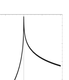
Figure 3: The behavior of the function $\mbox{Re}\,\hat{P}_{0}(\bar{\lambda})$ in the vicinity of $\bar{\lambda}=0$.

Excellent fits reveal the following expressions for $\Phi_{l}\,,\ \ (l=0,1,2,3,4,5)$:

$$\Phi_{0}(\bar{\lambda}) = 0.0570\frac{\log(-0.154\bar{\lambda})}{1+0.220(\log(-0.494\bar{\lambda}))^{2}}\,,$$

$$\Phi_{1}(\bar{\lambda}) = \frac{0.0212\log(-10.2\bar{\lambda})+0.00142(\log(-0.109\bar{\lambda}))^{3}}{1+0.128(\log(-1.09\bar{\lambda}))^{2}+0.0544(\log(-0.886\bar{\lambda}))^{4}}\,,$$

$$\Phi_{3}(\bar{\lambda}) = -0.0544\frac{\log(-0.367\bar{\lambda})}{1+0.641(\log(-0.513\bar{\lambda}))^{2}}\,,$$

$$\Phi_{4}(\bar{\lambda}) = \frac{-0.0722\log(-1.66\bar{\lambda})+0.00780(\log(-1.95\bar{\lambda}))^{3}}{1+0.212(\log(-1.90\bar{\lambda}))^{2}+0.0864(\log(-1.06\bar{\lambda}))^{4}}\,,$$

$$\Phi_{5}(\bar{\lambda}) = \frac{14.7\log(-0.505\bar{\lambda})-1.01(\log(-0.917\bar{\lambda}))^{3}-0.0172(\log(-0.0568\bar{\lambda}))^{5}}{1+5.84(\log(-0.0156\bar{\lambda}))^{2}+0.925(\log(-10.3\bar{\lambda}))^{4}+1.68(\log(-0.641\bar{\lambda}))^{6}}\,.$$

Fig. 4 shows for $\bar{\lambda}\geq 0$ plots of the $\mbox{Re}\,\Phi_{l}$, which are continuous across the cut, and $\mbox{Im}\,\Phi_{l}$, whose respective signs are chosen such as to minimize the value of $\bar{\lambda}>0$ where they first intersect with $\mbox{Re}\,\Phi_{l}$ (approach to the cut as $\bar{\lambda}=\mbox{Re}\,\bar{\lambda}\pm i\,0$).

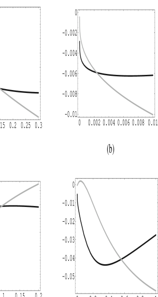
Figure 4: The real (black) and the imaginary (grey) part of the functions $\hat{P}_{l}(\bar{\lambda})$ for $l=0$ (a), $l=1$ (b), $l=2$ (c), $l=3$ (d), $l=4$ (e) and positive $\bar{\lambda}$.

Notice that $\mbox{Re}\,\Phi_{l}$ and $\mbox{Im}\,\Phi_{l}$ vanish precisely at $\bar{\lambda}=0$. Notice also that for $\bar{\lambda}\geq 0$ and in the vicinity of $\bar{\lambda}=0$ the modulus of $\mbox{Re}\,\Phi_{l}$ grows much more rapidly than the modulus of $\mbox{Im}\,\Phi_{l}$.

3.4 Interpretation of the results of Sec. 3.3

Due to the meromorphic nature of the functions $\Phi_{l}$ away from the cut along the positive-real axis and the fact that $\mbox{Re}\,\Phi_{l}$ is continuous across this cut we have no choice but to regard, up to a modification involving finitely many terms, the quantity

$$P_{\tiny\mbox{mass}}(\hat{\beta})\equiv\frac{\Lambda^{4}}{\sqrt{2}\,\pi^{\frac{3}{2}}\,{\hat{\beta}}^{\frac{5}{2}}}\,\mbox{Re}\,\sum^{L}_{l=0}a_{l}\,\hat{P}_{l}\left(\bar{\lambda}(\hat{\beta})\right)$$ (19)

as a unique prediction for the pressure exerted by the massive modes in the confining phase of an SU(2) Yang-Mills theory, compare with Eq. (6). We expect this pressure to be positive and rapidly growing for $\bar{\lambda}>0$, see [9] where the asymptotic expansion of Eq. (6) was used to predict the temperature dependence of the pressure for an ‘electron’ gas. For accurate numerical predictions the integer coefficients $a_{l}$ would have to be known. In a $\lambda\phi^{4}$-theory the algebraic dependence of the number of connected vacuum bubble diagrams on $n$ should be extractable from a numerical analysis of the ground-state energy of an anharmonic oscillator, see [12, 13].

It is important to realize that at $\hat{\beta}=\infty$ (or $T=0$ or $\bar{\lambda}=0$) we have $P_{\tiny\mbox{mass}}(\hat{\beta}=\infty)=0$. That is, the contribution to the cosmological constant arising from an SU(2) Yang-Mills theory at zero temperature is nil. Thus the according ‘tree-level’ result [1, 2], which relates to the zero of the effective potential for the vortex condensate ($\propto$ the ’t Hooft-loop expectation [1, 2]) survives the integration of fluctuations as performed in the present work.

But what about the imaginary part in $P_{\tiny\mbox{mass}}$? As is readily observed from Fig. 4 (and is easily proven analytically for all $l$) the modulus of $\mbox{Re}\,\Phi_{l}(\bar{\lambda})$ grows much faster than $|\mbox{Im}\,\Phi_{l}(\bar{\lambda})|$ with increasing $\bar{\lambda}$ starting at $\bar{\lambda}=0$. Thus for a certain range of small values $\hat{\beta}^{-1}$ the pressure $P_{\tiny\mbox{mass}}(\hat{\beta})$ is dominated by the real part.

The presence of a growing imaginary contamination signals an increasing deviation of the system from a thermodynamical behavior. Namely, we interprete the occurrence of a sign-indefinite imaginary part as an indication for the violation of a basic thermodynamical property: Spatial homogeneity. That is, the growth of the ratio $R\equiv\mbox{Im}\,P_{\tiny\mbox{mass}}/\mbox{Re}\,P_{\tiny\mbox{mass}}$ with increasing temperature is a measure for the increasing importance of turbulence-like phenomena in the plasma. At $R=1$ the thermodynamical description of the system fails badly; the system then is highly ‘nervous’ and close to the Hagedorn transition.

We believe that the so-predicted occurrence of sizably nonthermal behavior at sufficiently large temperature is the reason for the failure of stabilization of the magnetically confined plasma in tokamak experiments. This presumes that the description of the electron and its neutrino and their quantum mechanics [18] is based on a pure SU(2) Yang-Mills theory of scale $\Lambda=m_{e}=511\,$keV, see [1, 2, 9]. Notice that the electron and its neutrino are the only stable excitations in the confining phase of this theory, compare with Fig. 1. The occurrence of poorly understood microturbulences and internal transport barriers in tokamaks was reported for $\frac{T}{\Lambda}\sim 0.05\,...\,0.09$, see JET’s results and ITER’s design report.

4 Summary and Outlook

In the present work we have performed an in-principle calculation of the pressure of an SU(2) Yang-Mills theory at low temperature. In particular, we have shown that the pressure vanishes precisely at zero temperature. We have also demonstrated that nonthermal effects start to become sizable at a certain critical temperature $T_{*}$. Numerical predictions for $T_{*}$ and the dependence of the pressure on temperature need input about the precise algebraic dependence of the number of connected vacuum bubbles on the number $n\gg 1$ of vertices in a $\lambda\phi^{4}$-theory. Also, one would need to know these numbers for the first few $n$. We hope that this information will be available soon.

The tool employed to derive the above results is to show Borel summability of an asymptotic-series representation of the pressure at negative values of a coupling constant $\bar{\lambda}$ suitably defined for $T\geq 0$. The so-obtained functional dependence is meromorphic in the entire complex $\bar{\lambda}$-plane except for a branch cut along the positive-real axis. The crucial observation is that the real part of this function is continuous across the cut and that its modulus grows faster than that of the imaginary part for a certain range of increasing $\bar{\lambda}\geq 0$. The presence of the imaginary contamination signals a deviation from thermal equilibrium by local violations of spatial homogeneity (plasma turbulences). We believe that our results are of relevance in addressing the observed but poorly understood microturbulences and internal transport barriers ocurring in terrestial fusion experiments with magnetic plasma confinement.

The generalization of our SU(2) results to SU(3) is trivial since for SU(3) the number of vortex-loop species at a given time is just twice that of the SU(2) case.

References

- [1] R. Hofmann, Int. J. Mod. Phys. A 20, 4123 (2005), Erratum-ibid. A 21, 6515 (2006).
- [2] R. Hofmann, Mod. Phys. Lett. A 21, 999 (2006), Erratum-ibid. A 21, 3049 (2006).
- [3] R. Hofmann, hep-th/0507033.
- [4] R. Hofmann, hep-th/0607106, in proceedings of 7th Workshop on Continuous Advances in QCD, Minneapolis, Minnesota, 11-14 May 2006.
- [5] U. Herbst and R. Hofmann, hep-th/0411214 (unpublished).
- [6] R. Hofmann, hep-th/0609033.
- [7] R. Hofmann, hep-th/0507122 (unpublished).
- [8] R. Hofmann, hep-th/0508212 (unpublished).
- [9] F. Giacosa, R. Hofmann, and M. Schwarz, Mod. Phys. Lett. A 21, 2709 (2006).
- [10] G. ’t Hooft, Nucl. Phys. B 138, 1 (1978).
- [11] C. M. Bender and T. T. Wu, Phys. Rev. Lett. 37, 117 (1976).
- [12] C. M. Bender and T. T. Wu, Phys. Rev. 184, 1231 (1969).
- [13] C. M. Bender and T. T. Wu, Phys. Rev. Lett. 27, 461 (1971).
- [14] H. Kleinert and V. Schulte-Frohlinde, Critical Properties of -Theories, World Scientific Publishing Co. (2001).
- [15] D. Wood, Technical Report 15-92 (June, 1992), University of Kent computing Laboratory, University of Kent, Canterbury, UK.
- [16] L. Lewin, Polylogarithms and associated functions, Elsevier North Holland Inc. (1981), p. 236, Eq. (7.193).
- [17] E. Freitag and R. Busam, Funktionentheorie, Springer (1995), p. 204, Theorem 1.14.
- [18] F. Giacosa and R. Hofmann, Eur. Phys. J. C 50, 635 (2007).