hep-th/0610275 UT-06-22 IHES/P/06/53

Correlator of Fundamental and Anti-symmetric
Wilson Loops in AdS/CFT Correspondence

Ta-Sheng Tai^a and Satoshi Yamaguchi^b

^a Department of Physics, Faculty of Science, University of Tokyo

Hongo, Bunkyo-ku, Tokyo 113-0033, JAPAN

^b IHES, Le Bois-Marie, 35, Route de Chartres F-91440 Bures-sur-Yvette, FRANCE

We study the two circular Wilson loop correlator in which one is of anti-symmetric representation, while the other is of fundamental representation in 4-dimensional ${\cal N}=4$ super Yang-Mills theory. This correlator has a good AdS dual, which is a system of a D5-brane and a fundamental string. We calculated the on-shell action of the string, and clarified the Gross-Ooguri transition in this correlator. Some limiting cases are also examined.

1 Introduction and summary

The Wilson loop is one of the most interesting quantities which appeared in the AdS/CFT correspondence [1]. In the computation of the expectation value of the Wilson loop, the stringy effect (not just the supergravity) is essential. Actually, it is calculated on the AdS side as the on-shell action of a classical macroscopic string[2, 3] in the limit of large $N$ and large ’t Hooft coupling $\lambda=4\pi g_{s}N=g^{2}_{YM}N$.

Recently, certain D-brane pictures of Wilson loops have drawn wide attention because they are powerful in evaluating the Wilson loop of higher rank representation. The D3-brane with electric flux, which has already been investigated in [2], is found to describe Wilson loops of symmetric representations (or multiply wound Wilson loops) by Drukker and Fiol [4]. On the other hand, the Wilson loop of anti-symmetric representation is found to be described by a D5-brane with electric flux[5, 6, 7]. In both cases, the results show successful agreement with the gauge theory side calculations [8, 9]. Other further investigations along this line can be found in [10, 11, 12, 13, 14, 15].

One of the interesting phenomena in the AdS picture of Wilson loops is the phase transition, which occurs in the two Wilson loop correlator. This is first anticipated by Gross and Ooguri [16], and further explored in [17, 18, 19, 20, 21, 22, 23]. If the two loops are close enough, the classical string of annulus topology leads to the smallest action, which dominates the connected correlator. By contrast, when the two loops get far enough, two disk solution with massless propagating modes dominates the connected correlator. Between them, there exists a critical point.

In this paper, we study two concentric circular Wilson loop correlator of different representations, i.e. one is fundamental and the other is anti-symmetric. Because the circular anti-symmetric Wilson loop has a gravity dual as a D5-brane with electric flux, this correlator can thus be recognized as a system of a D5-brane and an F-string. More explicitly, it is realized as a string which propagates between the AdS boundary and the D5-brane.

Here let us summarize the results of this paper. We calculated the correlator by evaluating the on-shell action of the string worldsheet. This correlator also exibits the phase transition. The phase structure is shown in figures 3, 4 and 5. The critical surface of the phase transition is represented by a solid line. There is also a critical surface represented by a dashed line where the annulus solution becomes unstable.

The parameter $\Theta$ (direction in $S^{5}$) dependence is quite nontrivial and interesting. As easily seen from the figures 3, 4 and 5, as well as from the expression in section 3, the correlator has the symmetry $\Theta\to 2\theta_{k}-\Theta$, where $\theta_{k}$ is a function of $k$ as in eq.(3.4). Especially, the point $\Theta=2\theta_{k}-\pi$ looks similar to the point $\Theta=\pi$. At $\Theta=\pi$, it is always in the disk phase, since it is BPS even when two loops get on top of each other. On the other hand, $\Theta=2\theta_{k}-\pi$ is not a priori related to the BPS configuration, but it is always in the disk phase. This fact implies that overlapped loops at $\Theta=2\theta_{k}-\pi$ bear a similar nature to the BPS loops.

Another interesting feature related to $\Theta$ dependence is the maximum of the critical distance. The critical distance is maximal at $\Theta=\theta_{k}$. This is reasonable in the AdS picture since the D5-brane sits at $\theta=\theta_{k}$. However, it is rather misterious because the origin of $\theta_{k}$ is quite different from $\Theta$ on the gauge theory side. It should be interesting and useful to consider the origin of $\theta_{k}$ more geometrically on the gause theory side.

We also studied a couple of limiting cases. The solution of two fundamental Wilson loop correlator first examined by Zarembo[17] is recovered, meanwhile the Coulomb-like behavior is found when the separation is much smaller than the circle radii.

As a future work, the Yang-Mills side analysis like [24, 25] seems to be interesting. Correlators of Wilson loops of other representations by using the D3-brane [4] or supergravity solutions [26, 27] are as well worthy of study. Also, the extension to finite temperature cases is in progress.

The rest of this paper is organized as follows. In sec.2, the detailed setup is given. In sec.3, the AdS side calculation is performed through a series of elliptic integrals. Finally, in sec.4, we plotted the phase diagram, which visualizes clearly the Gross-Ooguri transition. Comments on these solutions are also provided, where known results appear as limiting cases. Some definitions and algebra involving elliptic integrals are added in the appendix A. The explicit forms of the Coulomb coefficients are shown in appendix B.

2 Setup

In $\mathcal{N}=4$ Super Yang-Mills theory, the Wilson loop is defined as

$$W_{\mathsf{R}}(C):=\operatorname*{{\rm Tr}}_{\mathsf{R}}\big{[}P\exp\oint_{C}d\tau(iA_{\mu}{\dot{x}}^{\mu}+\Phi_{I}n^{I}(\tau)|\dot{x}|)\big{]},$$ (2.1)

where $A_{\mu}$ is the gauge field, $\Phi_{I}$’s are six scalar fields, $C$ is a closed trajectory in 4-dimensional spacetime parameterized by $\tau$, $n_{I}$ is a 6-dimensional unit vector, and $\mathsf{R}$ is a representation of SU($N$). In this paper, we consider the following type of correlation function

$$\left\langle W_{A_{k}}(C_{1})W_{\Box}(C_{2})\right\rangle.$$ (2.2)

We take the trajectories $C_{1}$ and $C_{2}$ as two circles. Both of them are embedded in a 3-dimensional hyperplane of 4-dimensional space. They are parallel and the centers of them are on the axis which is orthogonal to the circles. If we introduce the Cartesian coordinate $x_{\mu}$, $C_{1}$ is expressed via $\tau$ as

$$x_{\mu}=(0,R_{1}\cos\tau,R_{1}\sin\tau,0),\qquad n^{I}=(1,0,0,0,0,0),$$ (2.3)

while $C_{2}$ is

$$x_{\mu}=(L,R_{2}\cos\tau,-R_{2}\sin\tau,0),\qquad n^{I}=(\cos\Theta,\sin\Theta,0,0,0,0),\qquad(0<L,~{}0\leq\Theta\leq\pi).$$ (2.4)

So parameters of this configuration are $R_{1},R_{2},L,\Theta$.

The correlator (2.2) factorizes in the leading term of the $1/N$ expansion. But this term does not depend on parameters $L,R_{1},R_{2},\Theta$. In order to see their dependence, the subleading terms become relevant. In other words, what we have to consider is the “connected correlator”

$$\left\langle W_{A_{k}}(C_{1})W_{\Box}(C_{2})\right\rangle_{conn}=\left\langle W_{A_{k}}(C_{1})W_{\Box}(C_{2})\right\rangle-\left\langle W_{A_{k}}(C_{1})\right\rangle\left\langle W_{\Box}(C_{2})\right\rangle.$$ (2.5)

As we will see later, it is convenient to define the function $V_{k}(R_{1},R_{2},L,\Theta)$ as

$$V_{k}(R_{1},R_{2},L,\Theta):=\frac{\left\langle W_{A_{k}}(C_{1})W_{\Box}(C_{2})\right\rangle-\left\langle W_{A_{k}}(C_{1})\right\rangle\left\langle W_{\Box}(C_{2})\right\rangle}{\left\langle W_{A_{k}}(C_{1})\right\rangle}.$$ (2.6)

On the AdS side, this correlation function is described by a system of a D5-brane and a fundamental string subject to certain boundary conditions. The D5-brane is rigid because it is much heavier than the fundamental string. By contrast, the string is flexible, so various kinds of contributions should be considered.

There are two possible leading contributions to $V_{k}$. One is a disk bounded by $C_{2}$ with massless propagating modes connecting the F-string and the D5-brane (see figure 1). The other is an annulus whose boundaries are attached to the D5-brane and $C_{2}$ (see figure 2). These two contributions are of the same order $\simeq{\cal O}(N^{0})$ in $1/N$ expansion. Their magnitudes are estimated by the on-shell action of the annulus and the disk, respectively, in large $\lambda$ limit.

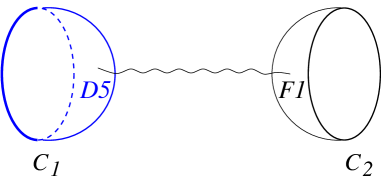
Figure 1: The schematical picture of the disk solution with massless propagating modes. The disk solution is of order $1/g_{s}$, the massless propagator is of order $g_{s}^{2}$ and the coupling to the D5-brane is of order $1/g_{s}$. Totally, the contribution is of order $g_{s}^{0}$, which is the same order as the annulus contribution.

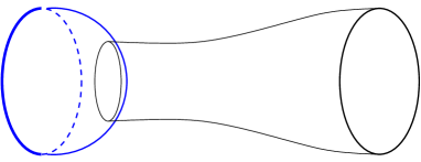
Figure 2: The schematical picture of the annulus. Since the D5-brane is much heavier than the fundamental string, the D5-brane is not deformed. The contribution from this annulus solution is as well of order $g_{s}^{0}$.

In summary, in large $\lambda$ limit, $V_{k}$ is approximated as

$$V_{k}(R_{1},R_{2},L,\Theta)=\exp(-S_{min}),$$ (2.7)

where $S_{min}$ is the global minimum of the string action. The classical on-shell action of the disk, which corresponds to a single circular Wilson loop, has been calculated in [28]. The result is

$$S_{disk,min}=-\sqrt{\lambda}.$$ (2.8)

The question now is the competition of (2.8) and that of the annulus. We will investigate the classical annulus solution and compare it with (2.8) in this paper.

Before doing this, we can make some observation upon using the conformal symmetry. There are certain constraints on the correlation function. For example, we have a relation from the dilatation

$$V_{k}(R_{1},R_{2},L,\Theta)=V_{k}(aR_{1},aR_{2},aL,\Theta),$$ (2.9)

where $a$ is a real positive parameter of the dilatation. We can also use the special conformal transformation with a vector parameter $b^{\mu}$

$$x^{\prime\mu}=\frac{x^{\mu}-b^{\mu}|x|^{2}}{1-2b^{\mu}x_{\mu}+|b|^{2}|x|^{2}}.$$ (2.10)

This special conformal transformation (2.10) along $x_{1}$, i.e. $b^{\mu}=(h,0,0,0)$ makes

$$\begin{aligned} &V_{k}(R_{1},R_{2},L,\Theta)=V_{k}(R_{1}^{\prime},R_{2}^{\prime},L^{\prime},\Theta),\\ &R_{1}^{\prime}=\frac{R_{1}}{1+h^{2}R_{1}^{2}},\qquad R_{2}^{\prime}=\frac{R_{2}}{1-2hL+h^{2}(L^{2}+R_{2}^{2})},\\ &L^{\prime}=\frac{L-h(L^{2}+R_{2}^{2})}{1-2hL+h^{2}(L^{2}+R_{2}^{2})}+\frac{hR_{1}^{2}}{1+h^{2}R_{1}^{2}}.\end{aligned}$$ (2.11)

Therefore, $V_{k}$ is a function of the invariant combination $\eta$ as

$$V_{k}(R_{1},R_{2},L,\Theta)=\widetilde{V}_{k}(\eta,\Theta),\qquad\eta=\frac{R_{1}^{2}+R_{2}^{2}+L^{2}}{2R_{1}R_{2}}.$$ (2.12)

On the AdS side, this simple dependence on $(\eta,\Theta)$ is not quite trivial. This is due to the introduction of the cutoff, which makes the conformal symmetry not manifest. In order to check this conformal symmetry, we keep the parameters $(R_{1},R_{2},L)$ generic in the calculation in the next section. We will find that the constraint (2.12) is actually satisfied.

3 Classical solution of the annulus

In this section, we will investigate the annulus solution. We use similar techniques employed by [17, 18, 19]. We write down the solution and the corresponding on-shell action. One can see the “phase structure” from the result.

3.1 Ansatz and equations of motion

In this paper, we use the following notation for $AdS_{5}\times S^{5}$ with radius $\sqrt{\alpha^{\prime}}\lambda^{1/4}$

$$ds^{2}=\frac{\alpha^{\prime}\sqrt{\lambda}}{y^{2}}(dy^{2}+dr^{2}+r^{2}d\varphi^{2}+dt^{2}+dx^{2})+\alpha^{\prime}\sqrt{\lambda}(d\theta^{2}+\sin^{2}\theta d\Omega_{4}^{2}).$$ (3.1)

The boundary of $AdS_{5}$ is at $y=0$. The coordinate $(r,\varphi,t,x)$ at the boundary is related to the Cartesian coordinate $x_{\mu}$ introduced in the previous section as

$$x_{1}=x,\qquad x_{2}=r\cos\varphi,\qquad x_{3}=r\sin\varphi,\qquad x_{4}=t.$$ (3.2)

The string dual of $W_{A_{k}}(C_{1})$ is a D5-brane [6, 7]. Its explicit form[29, 30] is expressed as

$$r^{2}+y^{2}=R_{1}^{2},\qquad\theta=\theta_{k},$$ (3.3)

where $R_{1}$ is the radius of $C_{1}$, and $\theta_{k}$ is related to $k$ as

$$\frac{k}{N}=\frac{1}{\pi}\left(\theta_{k}-\frac{1}{2}\sin 2\theta_{k}\right).$$ (3.4)

The gauge field excitation on the D5-brane worldvolume has the field strength

$${\cal F}_{y\varphi}=-i\cos\theta_{k}\frac{\alpha^{\prime}\sqrt{\lambda}R_{1}}{y^{2}},\qquad{\cal F}:=2\pi\alpha^{\prime}dA.$$ (3.5)

The worldsheet stretching between this D5-brane and $C_{2}$ is symmetric under the rotation $\varphi\to\varphi+\alpha,\ \alpha$: real constant parameter. Hence, we can assign this symmetry to our solution. The reparameterization degrees of freedom enable one to set the worldsheet coordinates as $(\sigma,\varphi)$, where $\varphi$ is the same as the spacetime $\varphi$. The ansatz used is written as

$$y =y(\sigma),\qquad r=r(\sigma),\qquad x=x(\sigma),\qquad\theta=\theta(\sigma).$$ (3.6)

In this ansatz, we include $\sigma$ dependence of $\theta$ because the two boundaries are separated in $S^{5}$ in general, i.e. the D5-brane is wrapped on an $S^{4}$ at $\theta=\theta_{k}$, while $C_{2}$ sits at a point $\theta=\Theta$ in $S^{5}$. This kind of separation in $S^{5}$ is first considered extensively in [21]. Their method of solving the equation of motion is applicable to the problem here, if one uses the conformal symmetry and simplifies the configuration. Here, however, we do not use the conformal symmetry to simplify the configuration. This is because one purpose of this calculation is to check the conformal symmetry.

The bulk part comes from the Nambu-Goto action

$$S_{bulk}=\frac{1}{2\pi\alpha^{\prime}}\int d\sigma d\varphi\sqrt{\det G},$$ (3.7)

where $G$ is the induced metric. Plugging (3.6) and integrating out $\varphi$, we obtain

$$S_{bulk}=\sqrt{\lambda}\int d\sigma\frac{r}{y^{2}}\sqrt{x^{\prime 2}+r^{\prime 2}+y^{\prime 2}+y^{2}\theta^{\prime 2}},$$ (3.8)

where prime ^′ denotes the $\sigma$ derivative.

At both boundaries, we need to include proper boundary terms. Let $\sigma=\sigma_{1}$ be the boundary on the D5-brane, whereas $\sigma=\sigma_{2}$ be the boundary at $C_{2}$ with $\sigma_{1}<\sigma_{2}$. At $\sigma=\sigma_{1}$, the boundary is constrained on the rigid D5-brane in (3.3), and should satisfy at least the following conditions

$$r^{2}+y^{2}=R_{1}^{2},\qquad x=0,\qquad\theta=\theta_{k}.$$ (3.9)

These are not all the conditions however. Due to the gauge field excitation in (3.5), we should add

$$\begin{aligned} S_{bdy,1}=i\oint_{\sigma=\sigma_{1}}d\varphi~{}A_{\varphi}~{}+(\text{constant})=\sqrt{\lambda}\cos{\theta_{k}}\left(1-\frac{R_{1}}{y}\right),~{}&&A_{\varphi}=\frac{1}{2\pi\alpha^{\prime}}i\cos{\theta_{k}}\frac{\alpha^{\prime}\sqrt{\lambda}R_{1}}{y}.\end{aligned}$$ (3.10)

The (constant) ensures that $S_{bdy,1}=0$ when $y=R_{1}$, where the circle of $\varphi$ shrinks to a point. The boundary condition is derived from the variational principle. The variation of the bulk action has boundary terms at $\sigma=\sigma_{1}$ as

$$\delta S_{bulk}|_{bdy,1}= -p_{r}\delta r-p_{y}\delta y-p_{x}\delta x-p_{\theta}\delta\theta.$$ (3.11)

The momenta $p$ are written as

$$p_{r}=\sqrt{\lambda}\frac{r}{y^{2}}\frac{r^{\prime}}{\sqrt{x^{\prime 2}+r^{\prime 2}+y^{\prime 2}+y^{2}\theta^{\prime 2}}},$$ (3.12)

$$p_{y}=\sqrt{\lambda}\frac{r}{y^{2}}\frac{y^{\prime}}{\sqrt{x^{\prime 2}+r^{\prime 2}+y^{\prime 2}+y^{2}\theta^{\prime 2}}},$$ (3.13)

$$p_{x}=\sqrt{\lambda}\frac{r}{y^{2}}\frac{x^{\prime}}{\sqrt{x^{\prime 2}+r^{\prime 2}+y^{\prime 2}+y^{2}\theta^{\prime 2}}},$$ (3.14)

$$p_{\theta}=\sqrt{\lambda}\frac{r\theta^{\prime}}{\sqrt{x^{\prime 2}+r^{\prime 2}+y^{\prime 2}+y^{2}\theta^{\prime 2}}}.$$ (3.15)

Due to $r^{2}+y^{2}=R_{1}$, it is convenient to rewrite (3.11) as

$$\delta S_{bulk}|_{bdy,1} =-\frac{1}{2}\left(\frac{p_{r}}{r}+\frac{p_{y}}{y}\right)\left(r\delta r+y\delta y\right)-\frac{1}{2}\left(\frac{p_{r}}{r}-\frac{p_{y}}{y}\right)\left(r\delta r-y\delta y\right)-p_{x}\delta x-p_{\theta}\delta\theta.$$ (3.16)

On the other hand, the variation of $S_{bdy,1}$ is written as (using the condition $r\delta r+y\delta y=0$)

$$\delta S_{bdy,1}=-\frac{1}{2}\sqrt{\lambda}\cos\theta_{k}\frac{R_{1}}{y^{3}}(r\delta r-y\delta y).$$ (3.17)

We obtain totally

$$\delta S_{bulk}|_{bdy,1}+\delta S_{bdy,1} =-\frac{1}{2}\left(\frac{p_{r}}{r}+\frac{p_{y}}{y}\right)\left(r\delta r+y\delta y\right)-\frac{1}{2}\left(\frac{p_{r}}{r}-\frac{p_{y}}{y}+\sqrt{\lambda}\cos\theta_{k}\frac{R_{1}}{y^{3}}\right)\left(r\delta r-y\delta y\right)$$

$$\qquad-p_{x}\delta x-p_{\theta}\delta\theta.$$ (3.18)

The first, third and fourth term vanish because of (3.9). From the second term, it can be seen that the additional boundary condition at $\sigma=\sigma_{1}$ is

$$\frac{p_{r}}{r}-\frac{p_{y}}{y}+\sqrt{\lambda}\cos\theta_{k}\frac{R_{1}}{y^{3}}=0.$$ (3.19)

Next, let us turn to the other boundary at $\sigma=\sigma_{2}$. Naively, the area of the minimal surface is infinite. It is necessary to introduce a cutoff at $y=\epsilon$ in order to regularize the action. We follow [31] and perform the Legendre transformation. This gives a boundary term

$$S_{bdy,2}=-p_{y}y-p_{\theta}(\theta-\Theta),~{}~{}~{}~{}\text{at}~{}\sigma=\sigma_{2}.$$ (3.20)

Now we solve the equations of motion subject to the above boundary conditions. Each equation of motion of $r,y,x,\theta$, respectively, derived from (3.8) can be listed as

$$\frac{1}{y^{2}}\sqrt{x^{\prime 2}+r^{\prime 2}+y^{\prime 2}+y^{2}\theta^{\prime 2}}-\partial_{\sigma}\left(\frac{r}{y^{2}}\frac{r^{\prime}}{\sqrt{x^{\prime 2}+r^{\prime 2}+y^{\prime 2}+y^{2}\theta^{\prime 2}}}\right)=0,$$ (3.21)

$$-2\frac{r}{y^{3}}\sqrt{x^{\prime 2}+r^{\prime 2}+y^{\prime 2}+y^{2}\theta^{\prime 2}}+\frac{r}{y}\frac{\theta^{\prime 2}}{\sqrt{x^{\prime 2}+r^{\prime 2}+y^{\prime 2}+y^{2}\theta^{\prime 2}}}-\partial_{\sigma}\left(\frac{r}{y^{2}}\frac{y^{\prime}}{\sqrt{x^{\prime 2}+r^{\prime 2}+y^{\prime 2}+y^{2}\theta^{\prime 2}}}\right)=0,$$ (3.22)

$$\partial_{\sigma}\left(\frac{r}{y^{2}}\frac{x^{\prime}}{\sqrt{x^{\prime 2}+r^{\prime 2}+y^{\prime 2}+y^{2}\theta^{\prime 2}}}\right)=0,$$ (3.23)

$$\partial_{\sigma}\left(\frac{r\theta^{\prime}}{\sqrt{x^{\prime 2}+r^{\prime 2}+y^{\prime 2}+y^{2}\theta^{\prime 2}}}\right)=0.$$ (3.24)

Following [17, 18], we integrate (3.23), (3.24) and fix the reparameterization of $\sigma$ as $x=\sigma$ to obtain

$$\frac{r}{y^{2}}\frac{1}{\sqrt{1+r^{\prime 2}+y^{\prime 2}+y^{2}\theta^{\prime 2}}}=\ell,$$ (3.25)

$$\frac{r\theta^{\prime}}{\sqrt{1+r^{\prime 2}+y^{\prime 2}+y^{2}\theta^{\prime 2}}}=m,$$ (3.26)

where $\ell$ and $m$ are integration constants. We can assume $\ell>0$ without loss of generality. Plugging these into (3.21) and (3.22), we obtain

$$\frac{r}{\ell^{2}y^{4}}-r^{\prime\prime} =0,$$ (3.27)

$$-\frac{2r^{2}}{\ell^{2}y^{5}}+\frac{m^{2}}{\ell^{2}y^{3}}-y^{\prime\prime} =0,$$ (3.28)

and they combine to be

$$0=1+r^{\prime 2}+y^{\prime 2}-\frac{r^{2}}{\ell^{2}y^{4}}+\frac{m^{2}}{\ell^{2}y^{2}}.$$ (3.29)

Adding (3.27) multiplied by $r$ to (3.28) multiplied by $y$ leads to

$$(r^{2}+y^{2})^{\prime\prime}+2=0.$$ (3.30)

This equation is integrated to be

$$r^{2}+y^{2}+(x+c)^{2}=a^{2},$$ (3.31)

where $a$ and $c$ are integration constants. At $x=0$ (D5-brane side), $r^{2}+y^{2}=R_{1}^{2}$ leads to

$$a^{2}-c^{2}=R_{1}^{2},$$ (3.32)

while at $x=L$ (AdS boundary,) $r=R_{2}$ and $y=0$ lead to

$$a^{2}-(L+c)^{2}=R_{2}^{2}.$$ (3.33)

Based on these, $a$ and $c$ can be expressed in terms of $R_{1},R_{2},L$ as

$$c=\frac{R_{1}^{2}-R_{2}^{2}-L^{2}}{2L},\qquad a=\frac{\sqrt{(R_{1}^{2}+R_{2}^{2}+L^{2})^{2}-4R_{1}^{2}R_{2}^{2}}}{2L}.$$ (3.34)

By using the trigonometric parameterization

$$r=\sqrt{a^{2}-(x+c)^{2}}\cos\phi,~{}~{}~{}~{}y=\sqrt{a^{2}-(x+c)^{2}}\sin\phi,\qquad 0\leq\phi\leq\frac{\pi}{2},$$ (3.35)

(3.29) becomes

$$\phi^{\prime}=\pm\left(\frac{a}{a^{2}-(x+c)^{2}}\right)\frac{\sqrt{\cos^{2}\phi-m^{2}\sin^{2}\phi-\ell^{2}a^{2}\sin^{4}\phi}}{\ell a\sin^{2}\phi}.$$ (3.36)

Furthermore, the boundary condition (3.19) can be rewritten as a constraint on $\phi_{1}:=\phi(0)$ and $\phi^{\prime}(0)$ as

$$\phi^{\prime}(0)=\cos\theta_{k}\frac{\sin\phi_{1}}{\ell R_{1}^{2}\cos^{2}\phi_{1}},$$ (3.37)

where we have used (3.35). Also, (3.37) and (3.36) lead to the expression of $\phi_{1}$ as

$$\sin^{2}\phi_{1}=\frac{-(m^{2}+\sin^{2}\theta_{k})+\sqrt{(m^{2}+\sin^{2}\theta_{k})^{2}+4\ell^{2}a^{2}\sin^{2}\theta_{k}}}{2\ell^{2}a^{2}}.$$ (3.38)

Finally, (3.26) can be rewritten as

$$\theta^{\prime}=\frac{m}{\ell(a^{2}-(x+c)^{2})\sin^{2}\phi}$$ (3.39)

by using (3.25) and (3.35). This and (3.36) together lead to

$$\frac{d\phi}{d\theta}=\frac{\phi^{\prime}}{\theta^{\prime}}=\pm\frac{1}{m}\sqrt{\cos^{2}\phi-m^{2}\sin^{2}\phi-\ell^{2}a^{2}\sin^{4}\phi}.$$ (3.40)

Now, we have almost done. Note that (3.36) and (3.40) can be easily integrated. The remaining subtlety is to choose the right branch from them. At $x=0$, we find that the sign of $\phi^{\prime}(0)$ is determined by the sign of $\cos\theta_{k}$ from (3.37). We will examine two cases: $\theta_{k}>\pi/2$ and $\theta_{k}<\pi/2$ in turn. The case of $\theta_{k}=\pi/2$ is realized as the limit of either case.

3.2 $\theta_{k}>\pi/2$: monotonically decreasing $\phi$

When $\theta_{k}>\pi/2$, $\phi^{\prime}(0)$ is negative by virture of (3.37), i.e. around $x=0$, $\phi$ decreases. Defining what inside the square root in (3.36) as a function of $\phi$ :

$${\cal H}(\phi):=\cos^{2}\phi-m^{2}\sin^{2}\phi-\ell^{2}a^{2}\sin^{4}\phi,$$ (3.41)

we see that ${\cal H}(\phi)$ is a monotonically decreasing function on $0\leq\phi\leq\pi/2$, and ${\cal H}(\phi_{1})>0$ according to (3.38). Hence as $\phi$ decreases, ${\cal H}$ becomes bigger and never reaches the branching point ${\cal H}=0$. Therefore, $\phi(x)$ is a monotonically decreasing function over $0\leq x\leq L$. We thus take the minus sign in (3.36), (3.40), and then integrate them to obtain

$$\int_{\phi_{1}}^{\phi}\frac{\ell a\sin^{2}\psi d\psi}{\sqrt{\cos^{2}\psi-m^{2}\sin^{2}\psi-\ell^{2}a^{2}\sin^{4}\psi}}=-\frac{1}{2}\log\frac{a+x+c}{a-x-c}+\frac{1}{2}\log\frac{a+c}{a-c},$$ (3.42)

$$\int_{\phi_{1}}^{\phi}\frac{md\psi}{\sqrt{\cos^{2}\psi-m^{2}\sin^{2}\psi-\ell^{2}a^{2}\sin^{4}\psi}}=-\theta+\theta_{k}.$$ (3.43)

Note that $\phi(x)$ and $\theta(x)$ can be completely fixed by solving the above equations implemented with the boundary conditions :

$$\phi(L)=0,\qquad\theta(L)=\Theta,$$ (3.44)

which in turn determine $m$ and $\ell$. To see this more explicitly, it is convenient to introduce

$$f(m,\ell a) =\int_{0}^{\phi_{1}}\frac{\ell a\sin^{2}\psi d\psi}{\sqrt{\cos^{2}\psi-m^{2}\sin^{2}\psi-\ell^{2}a^{2}\sin^{4}\psi}},$$ (3.45)

$$g(m,\ell a) =\int_{0}^{\phi_{1}}\frac{md\psi}{\sqrt{\cos^{2}\psi-m^{2}\sin^{2}\psi-\ell^{2}a^{2}\sin^{4}\psi}}.$$ (3.46)

Rewriting the L.H.S. of (3.42) at $x=L$ via (3.34) into

$$\begin{aligned} -\frac{1}{2}\log\frac{a+L+c}{a-L-c}+\frac{1}{2}\log\frac{a+c}{a-c}&=-\log\frac{R_{1}^{2}+R_{2}^{2}+L^{2}+\sqrt{(R_{1}^{2}-R_{2}^{2})^{2}+L^{4}+2L^{2}(R_{1}^{2}+R_{2}^{2})}}{2R_{1}R_{2}}\\ &=-\log\left[\eta+\sqrt{\eta^{2}-1}\right],\end{aligned}$$ (3.47)

where $\eta$ is defined in (2.12), we can re-express (3.44) as

$$\cosh[f(m,\ell a)]=\eta,\qquad g(m,\ell a)=\Theta-\theta_{k}.$$ (3.48)

Namely, $m$ and $\ell a$ are determined in terms of $\eta,\Theta$ if exist. Let us compute the on-shell action. The bulk action (3.8) now takes the form

$$S_{bulk}=\sqrt{\lambda}\int_{0}^{L}dx\frac{r}{y^{2}}\sqrt{1+r^{\prime 2}+y^{\prime 2}+y^{2}\theta^{\prime 2}}=\sqrt{\lambda}\int^{\phi_{1}}_{\frac{\epsilon}{R_{2}}}\frac{d\phi\cot^{2}\phi}{\sqrt{\cos^{2}\phi-m^{2}\sin^{2}\phi-{\ell^{2}a^{2}}\sin^{4}\phi}},$$ (3.49)

where we have put a cutoff at $y=\epsilon$. We ignore terms which vanish when $\epsilon\to 0$. Also, there are two boundary terms

$$x=0,~{}~{}~{}~{}S_{bdy,1}=\sqrt{\lambda}\cos\theta_{k}(1-\csc\phi_{1}),$$ (3.50)

$$x=L,~{}~{}~{}~{}S_{bdy,2}=-\sqrt{\lambda}\frac{R_{2}}{\epsilon},$$ (3.51)

from (3.10) and (3.20), respectively. The total on-shell action is $S_{tot}=S_{bulk}+S_{bdy,1}+S_{bdy,2}$.

Here we summarize the result of this subsection. When $\theta_{k}>\pi/2$, the on-shell action can be written by using the formulas in appendix A.2 as

$$\begin{aligned} \frac{S_{tot}}{\sqrt{\lambda}}=&[(m^{2}+1)^{2}+4\ell^{2}a^{2}]^{1/4}\Bigg{[}-\cot\chi(\phi_{1})\sqrt{1-\kappa^{2}\sin^{2}\chi(\phi_{1})}-E(\chi(\phi_{1}),\kappa)\\ &\qquad\qquad\qquad\qquad+(1-\kappa^{2})F(\chi(\phi_{1}),\kappa)\Bigg{]}+\cos\theta_{k}(1-\csc\phi_{1}).\end{aligned}$$ (3.52)

Note that $\phi_{1}$ is defined in (3.38), whereas $\chi(\phi),\kappa$ and $C$ are defined in (A.17). Here $F$ and $E$ are the elliptic integrals of the first and second kind, respectively. The integration constants $m,\ell a$ are determined by

$$\operatorname{{\rm arccosh}}\eta =\frac{(m^{2}+1)+\sqrt{(m^{2}+1)^{2}+4\ell^{2}a^{2}}}{2\ell a\left[(m^{2}+1)^{2}+4\ell^{2}a^{2}\right]^{1/4}}\left[\Pi(\chi(\phi_{1}),C,\kappa)-F(\chi(\phi_{1}),\kappa)\right],$$ (3.53)

$$\Theta-\theta_{k} =m[(m^{2}+1)^{2}+4\ell^{2}a^{2}]^{-1/4}F(\chi(\phi_{1}),\kappa),$$ (3.54)

where $\Pi$ is the elliptic integral of the third kind. We found that this result satisfies the conformal symmetry condition indicated in (2.12).

3.3 $\theta_{k}<\pi/2$: increasing and decreasing $\phi$

When $\theta_{k}<\pi/2$, $\phi^{\prime}(0)$ is positive by virtue of (3.37). Note that $\phi$ keeps increasing from $x=0$ (during when ${\cal H}$ in (3.41) decreases) untill the branching point (${\cal H}=0$) is reached at $x=x_{0}$. This causes a sign change in (3.36) and (3.40) such that $\phi$ starts to decrease all the way to zero at $x=L$. Consequently, we take the plus branch for $x\leq x_{0}$, and the minus branch for $x\geq x_{0}$ in (3.36) and (3.40).

It is convenient to define $\phi_{0}:=\phi(x_{0})$, which satisfies ${\cal H}(\phi_{0})=0$ and can be solved as

$$\sin^{2}\phi_{0}=\frac{-(m^{2}+1)+\sqrt{(m^{2}+1)^{2}+4\ell^{2}a^{2}}}{2\ell^{2}a^{2}}.$$ (3.55)

When $x\leq x_{0}$, integrating (3.36) and (3.40) gives

$$\int_{\phi_{1}}^{\phi}\frac{\ell a\sin^{2}\psi d\psi}{\sqrt{\cos^{2}\psi-m^{2}\sin^{2}\psi-\ell^{2}a^{2}\sin^{4}\psi}}=\frac{1}{2}\log\frac{a+x+c}{a-x-c}-\frac{1}{2}\log\frac{a+c}{a-c},$$ (3.56)

$$\int_{\phi_{1}}^{\phi}\frac{md\psi}{\sqrt{\cos^{2}\psi-m^{2}\sin^{2}\psi-\ell^{2}a^{2}\sin^{4}\psi}}=\theta-\theta_{k}.$$ (3.57)

On the other hand, when $x\geq x_{0}$,

$$\left(\int_{\phi_{1}}^{\phi_{0}}-\int_{\phi_{0}}^{\phi}\right)\frac{\ell a\sin^{2}\psi d\psi}{\sqrt{\cos^{2}\psi-m^{2}\sin^{2}\psi-\ell^{2}a^{2}\sin^{4}\psi}}=\frac{1}{2}\log\frac{a+x+c}{a-x-c}-\frac{1}{2}\log\frac{a+c}{a-c},$$ (3.58)

$$\left(\int_{\phi_{1}}^{\phi_{0}}-\int_{\phi_{0}}^{\phi}\right)\frac{md\psi}{\sqrt{\cos^{2}\psi-m^{2}\sin^{2}\psi-\ell^{2}a^{2}\sin^{4}\psi}}=\theta-\theta_{k}.$$ (3.59)

We again define

$$\tilde{f}(m,\ell a) =\left(\int_{\phi_{1}}^{\phi_{0}}+\int_{0}^{\phi_{0}}\right)\frac{\ell a\sin^{2}\psi d\psi}{\sqrt{\cos^{2}\psi-m^{2}\sin^{2}\psi-{\ell^{2}a^{2}}\sin^{4}\psi}},$$ (3.60)

$$\tilde{g}(m,\ell a) =\left(\int_{\phi_{1}}^{\phi_{0}}+\int_{0}^{\phi_{0}}\right)\frac{md\psi}{\sqrt{\cos^{2}\psi-m^{2}\sin^{2}\psi-{\ell^{2}a^{2}}\sin^{4}\psi}}$$ (3.61)

as before in order to incorporate the boundary condition (3.44). (3.58), (3.59) and (3.44) lead to

$$\eta=\cosh[\tilde{f}(m,\ell a)],\qquad\tilde{g}(m,\ell a)=\Theta-\theta_{k}.$$ (3.62)

Here, $m$ and $\ell a$ are determined in terms of $\eta,\Theta$ if exist. The on-shell action $S_{tot}$ contains the bulk part

$$\begin{aligned} S_{bulk}&=\sqrt{\lambda}\left(\int_{\phi_{1}}^{\phi_{0}}+\int_{\frac{\epsilon}{R_{2}}}^{\phi_{0}}\right)\frac{d\phi\cot^{2}\phi}{\sqrt{\cos^{2}\phi-m^{2}\sin^{2}\phi-{\ell^{2}a^{2}}\sin^{4}\phi}}\end{aligned}$$ (3.63)

as well as boundary terms which are the same as (3.50) and (3.51).

We summarize the result of this subsection. When $\theta_{k}<\pi/2$, the on-shell action can be written by using the formulas in appendix A.2 as

$$\begin{aligned} \frac{S_{tot}}{\sqrt{\lambda}}=&[(m^{2}+1)^{2}+4\ell^{2}a^{2}]^{1/4}\Bigg{[}\cot\chi(\phi_{1})\sqrt{1-\kappa^{2}\sin^{2}\chi(\phi_{1})}\\ &+E(\chi(\phi_{1}),\kappa)-(1-\kappa^{2})F(\chi(\phi_{1}),\kappa)-2E(\kappa)+2(1-\kappa^{2})K(\kappa)\Bigg{]}+\cos\theta_{k}(1-\csc\phi_{1}),\end{aligned}$$ (3.64)

where $\phi_{1}$ is defined in (3.38), while $\chi(\phi),\kappa$, and $C$ are defined in (A.17). The integration constants $m,\ell a$ are determined by

$$\operatorname{{\rm arccosh}}\eta=\frac{(m^{2}+1)+\sqrt{(m^{2}+1)^{2}+4\ell^{2}a^{2}}}{2\ell a\left[(m^{2}+1)^{2}+4\ell^{2}a^{2}\right]^{1/4}}\left[2\Pi(C,\kappa)-2K(\kappa)-\Pi(\chi(\phi_{1}),C,\kappa)+F(\chi(\phi_{1}),\kappa)\right],$$ (3.65)

$$\Theta-\theta_{k}=m[(m^{2}+1)^{2}+4\ell^{2}a^{2}]^{-1/4}[2K(\kappa)-F(\chi(\phi_{1}),\kappa)].$$ (3.66)

Again, the conformal symmetry condition in (2.12) is satisfied.

4 Comments on the solutions

4.1 Gross-Ooguri phase transition

Let us consider the Gross-Ooguri (GO) phase transition here. We compare (3.52)-(3.54) (or (3.64)-(3.66), when $\theta_{k}<\pi/2$) and (2.8). We are also interested in how far the annulus solution can stretch along $\eta$. For example, when $\theta_{k}>\pi/2$, the annulus solution exists, if and only if (3.53) and (3.54) can be solved by some $(m,\ell a)$ for a given $(\eta,\Theta)$ pair.

Figures 3, 4 and 5 present the phase diagrams plotted against the $\eta$-$\Theta$ plane at $\theta_{k}=\pi/2$, $\ 2\pi/3$ and $\ \pi/3$, respectively. The black solid line indicates the critical line of the GO phase transition. The red dashed line stands for the critical line where the annulus solution becomes unstable.

One finds that $\Theta=\pi$ is always in the disk phase. This observation has a good explanation. When $\Theta=\pi$, two loops get overlapped ($\eta=1$) so that this configuration becomes BPS. Therefore, the annulus solution does not exist.

The solution obtained in the previous section has a “duality” for a fixed $k$, i.e. $(\Theta,\eta)\to(2\theta_{k}-\Theta,\eta)$. Consequently, for $k\geq N/2$ ($\theta_{k}\geq\pi/2$), $\Theta\leq 2\theta_{k}-\pi$ is always in the disk phase. In paticular, the point $\Theta=2\theta_{k}-\pi,\ \eta=0$ bears a similar nature to the BPS point $\Theta=\pi,\ \eta=0$ in the approximation used here.

In addition, $\Theta$ dependence of the phase diagram is interesting. The critical distance marks a maximum at $\Theta=\theta_{k}$ when $\theta_{k}$ is fixed. This fact is quite reasonable from the AdS point of view. However, it is rather mysterious from the gauge theory side, since $\Theta$ and $\theta_{k}$ have rather different origins; $\Theta$ is the direction of the scalar as in (2.4), while $\theta_{k}$ is determined by the rank of the anti-symmetric representation as in (3.4). To consider this fact from the gauge theory is an interesting future work.

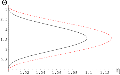
Figure 3: Phase diagram on $\eta$-$\Theta$ plane with $\theta_{k}=\pi/2$. The solid black line indicates the critical line of the GO transition. Inside (outside) the solid line, the annulus (disk) solution dominates the connected correlator. The red dashed line represents the critical line where the annulus solution becomes unstable. The annulus solution does not exist outside the red dashed line.

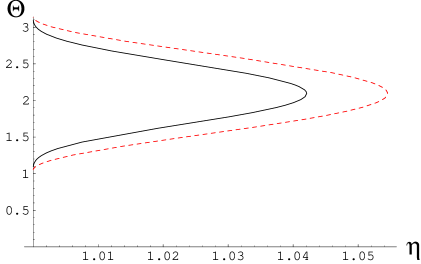
Figure 4: Phase diagram on $\eta$-$\Theta$ plane with $\theta_{k}=2\pi/3$.

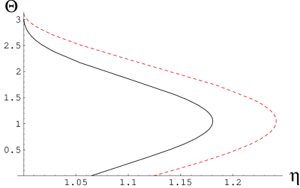
Figure 5: Phase diagram on $\eta$-$\Theta$ plane with $\theta_{k}=\pi/3$.

4.2 $k=1$

It is illuminating to check some limiting aspects of the above solutions. When $k=1$, the $k$-th anti-symmetric representation reduces to the fundamental one. Assuming $k=1$, one may expect (3.64)-(3.66) reproduce the correlator of two fundamental loops. We will see this is actually the case. It is nontrivial in the sense that the D5-brane picture of the anti-symmetric loop is valid only when $k$ is large and comparable to $N$. From (3.4), it is seen that $\lim_{k\rightarrow 1}\theta_{k}\cong\left(\frac{3\pi}{2N}\right)^{1/3}\ll 1$. Due to $\theta_{k}\ll 1$, one finds $\phi_{1}\ll 1$ by using (3.38). This means that the endpoint on the D5-brane is drawn closely to the AdS boundary.

Taking these facts into account, we can express the results (3.64)-(3.66) for $k=1$ as

$$\begin{aligned} S_{tot}=&\sqrt{\lambda}+2\sqrt{\lambda}[(m^{2}+1)^{2}+4\ell^{2}a^{2}]^{1/4}\left[-E(\kappa)+(1-\kappa^{2})K(\kappa)\right]\end{aligned}$$ (4.1)

$$\operatorname{{\rm arccosh}}\eta=\frac{(m^{2}+1)+\sqrt{(m^{2}+1)^{2}+4\ell^{2}a^{2}}}{\ell a\left[(m^{2}+1)^{2}+4\ell^{2}a^{2}\right]^{1/4}}\left[\Pi(C,\kappa)-K(\kappa)\right],$$ (4.2)

$$\Theta=2m[(m^{2}+1)^{2}+4\ell^{2}a^{2}]^{-1/4}K(\kappa).$$ (4.3)

Recall that $S_{tot}$ is identified with $-\log V_{k}$ in (2.7). The first term in $S_{tot}$ is interpreted as the contribution from the denominator in (2.6). The second term in (4.1) is completely the same as the one in the correlator of two fundamental Wilson loops, see [21]. If one takes further the limit $\Theta\to 0$ in the above expression, it reproduces the results of [17, 18, 19].

4.3 Limit to anti-parallel lines

When $R_{1}=R_{2}\gg L$, the Wilson loop correlator reduces to the anti-parallel lines. In this case, one expects that the correlator exhibits the Coulomb’s law as

$$-\log V_{k}(R_{1},R_{2},L,\Theta)\cong 2\pi R_{2}\frac{M}{L},$$ (4.4)

where $M$ is a constant determined by $k$ and $\Theta$. In terms of $\ell$ and $m$, this limit is realized via $\ell a\to\infty$ with $\gamma=\frac{m^{2}}{2\ell a}$ fixed. The explicit form of the coefficient $M$ is written down in appendix B.

Acknowledgements

We would like to thank Changhyun Ahn, Yosuke Imamura, Feng-Li Lin, Yutaka Matsuo, Nikita Nekrasov, Soo-Jong Rey and Jung-Tay Yee for useful discussions and comments. The work of S.Y. was supported in part by the European Research Training Network contract 005104 “ForcesUniverse.”

Appendix A Elliptic integrals

A.1 Definitions and some formulas of the standard elliptic integrals

$$F(\varphi,k):=\int_{0}^{\sin\varphi}dz\frac{1}{\sqrt{(1-z^{2})(1-k^{2}z^{2})}},$$ (A.1)

$$E(\varphi,k):=\int_{0}^{\sin\varphi}dz\sqrt{\frac{1-k^{2}z^{2}}{1-z^{2}}},$$ (A.2)

$$\Pi(\varphi,C,k):=\int_{0}^{\sin\varphi}dz\frac{1}{(1-Cz^{2})\sqrt{(1-z^{2})(1-k^{2}z^{2})}}.$$ (A.3)

Complete elliptic integrals are

$$K(k):=F(\pi/2,k),\qquad E(k):=E(\pi/2,k),\qquad\Pi(C,k):=\Pi(\pi/2,C,k).$$ (A.4)

When $C=k^{2}$, the third elliptic integral is related to the second one as

$$\Pi(\varphi,k^{2},k)=\frac{1}{1-k^{2}}E(\varphi,k)-\frac{k^{2}}{1-k^{2}}\frac{\sin\varphi\cos\varphi}{\sqrt{1-k^{2}\sin^{2}\varphi}}.$$ (A.5)

Let $a,b,c,d$ be four real constants which satisfies $a<b<c<d$. We assume the real variable $u$ satisfies $b\leq u\leq c$. If two variable $u$ and $z$ are related as

$$z^{2}:=\frac{(c-a)(u-b)}{(c-b)(u-a)},\quad\text{or}\quad u=\frac{(c-a)b-(c-b)az^{2}}{(c-a)-(c-b)z^{2}},$$ (A.6)

there is a 1-form relation

$$\frac{du}{\sqrt{(u-a)(u-b)(u-c)(u-d)}}=\frac{2}{\sqrt{(c-a)(d-b)}}\frac{dz}{\sqrt{(1-z^{2})(1-k^{2}z^{2})}},$$ (A.7)

$$k^{2}:=\frac{(c-b)(d-a)}{(c-a)(d-b)}.$$ (A.8)

We obtain the following formula.

$$\int_{b}^{v}\frac{du}{\sqrt{(u-a)(u-b)(u-c)(u-d)}}=\frac{2}{\sqrt{(c-a)(d-b)}}F(\varphi,k),$$ (A.9)

$$\sin\varphi:=\frac{(c-a)(v-b)}{(c-b)(v-a)}.$$ (A.10)

$$\int_{b}^{v}du\sqrt{\frac{(u-b)}{(u-a)(u-c)(u-d)}}=\frac{2(b-a)}{\sqrt{(c-a)(d-b)}}\left[\Pi(\varphi,C,k)-F(\varphi,k)\right],$$ (A.11)

$$C=\frac{c-b}{c-a}.$$ (A.12)

Let $\delta$ be a small number.

$$\int_{b+\delta}^{v} \frac{1}{(u-b)\sqrt{(u-a)(u-b)(u-c)(u-d)}}=$$

$$\frac{2}{\sqrt{(c-a)(d-b)}}\Bigg{\{}\sqrt{\frac{c-a}{(c-b)(b-a)}}\frac{1}{\sqrt{\delta}}-\frac{(c-a)}{(c-b)(b-a)}\cot\varphi\sqrt{1-k^{2}\sin^{2}\varphi}$$

$$\qquad\qquad-\frac{(c-a)}{(c-b)(b-a)}E(\varphi,k)+\frac{1}{c-b}F(\varphi,k)\Bigg{\}}+(\text{terms vanishing when }\delta\to 0).$$ (A.13)

In order to derive this formula, the relation

$$\frac{1}{z^{2}\sqrt{(1-z^{2})(1-k^{2}z^{2})}}=\frac{d}{dz}\left[\frac{-1}{z}\sqrt{(1-z^{2})(1-k^{2}z^{2})}\right]+\sqrt{\frac{1-k^{2}z^{2}}{1-z^{2}}}+\sqrt{(1-z^{2})(1-k^{2}z^{2})}$$ (A.14)

is useful.

A.2 Expressions of some integrals in terms of the standard elliptic integrals

$$u=\sin^{2}\psi,\qquad v=\sin^{2}\phi,\qquad\beta_{\pm}=\frac{-(m^{2}+1)\pm\sqrt{(m^{2}+1)^{2}+4\ell^{2}a^{2}}}{2\ell^{2}a^{2}},$$ (A.15)

where $\beta_{-}<0\leq v\leq\beta_{+}<1$, and

$$\frac{d\psi}{\sqrt{\cos^{2}\psi-m^{2}\sin^{2}\psi-\ell^{2}a^{2}\sin^{4}\psi}}=\frac{du}{2\ell a\sqrt{(u-\beta_{-})u(u-\beta_{+})(u-1)}}.$$ (A.16)

$$\kappa:=\sqrt{\frac{\beta_{+}(1-\beta_{-})}{\beta_{+}-\beta_{-}}},\qquad C:=\frac{\beta_{+}}{\beta_{+}-\beta_{-}},\qquad\chi(\phi):=\sin^{-1}\sqrt{\frac{(\beta_{+}-\beta_{-})\sin^{2}\phi}{\beta_{+}(\sin^{2}\phi-\beta_{-})}}.$$ (A.17)

$$\begin{aligned} &\int_{0}^{\phi}d\psi\frac{\ell a\sin^{2}\psi d\psi}{\sqrt{\cos^{2}\psi-m^{2}\sin^{2}\psi-\ell^{2}a^{2}\sin^{4}\psi}}=\frac{1}{2}\int_{0}^{v}du\sqrt{\frac{u}{(u-\beta_{-})(u-\beta_{+})(u-1)}}\\ &=\frac{(m^{2}+1)+\sqrt{(m^{2}+1)^{2}+4\ell^{2}a^{2}}}{2\ell a\left[(m^{2}+1)^{2}+4\ell^{2}a^{2}\right]^{1/4}}\left[\Pi(\chi(\phi),C,\kappa)-F(\chi(\phi),\kappa)\right].\end{aligned}$$ (A.18)

$$\begin{aligned} &\int_{0}^{\phi}d\psi\frac{md\psi}{\sqrt{\cos^{2}\psi-m^{2}\sin^{2}\psi-\ell^{2}a^{2}\sin^{4}\psi}}=\frac{1}{2\ell a}\int_{0}^{v}du\frac{m}{\sqrt{(u-\beta_{-})u(u-\beta_{+})(u-1)}}\\ &=m[(m^{2}+1)^{2}+4\ell^{2}a^{2}]^{-1/4}F(\chi(\phi),\kappa).\end{aligned}$$ (A.19)

$$\begin{aligned} &\int_{\frac{\epsilon}{R_{2}}}^{\phi}d\psi\frac{\cot^{2}\psi d\psi}{\sqrt{\cos^{2}\psi-m^{2}\sin^{2}\psi-\ell^{2}a^{2}\sin^{4}\psi}}=\frac{1}{2\ell a}\int_{\frac{\epsilon^{2}}{R_{2}^{2}}}^{v}du\frac{1-u}{u\sqrt{(u-\beta_{-})u(u-\beta_{+})(u-1)}}\\ &=\frac{R_{2}}{\epsilon}+[(m^{2}+1)^{2}+4\ell^{2}a^{2}]^{1/4}\left[-\cot\chi(\phi)\sqrt{1-\kappa^{2}\sin^{2}\chi(\phi)}-E(\chi(\phi),\kappa)+(1-\kappa^{2})F(\chi(\phi),\kappa)\right].\end{aligned}$$ (A.20)

When $\phi=\phi_{0}$, each integral becomes a complete elliptic integral, i.e.

$$\int_{0}^{\phi_{0}}d\psi\frac{\ell a\sin^{2}\psi d\psi}{\sqrt{\cos^{2}\psi-m^{2}\sin^{2}\psi-\ell^{2}a^{2}\sin^{4}\psi}} =\frac{(m^{2}+1)+\sqrt{(m^{2}+1)^{2}+4\ell^{2}a^{2}}}{2\ell a\left[(m^{2}+1)^{2}+4\ell^{2}a^{2}\right]^{1/4}}\left[\Pi(C,\kappa)-K(\kappa)\right],$$ (A.21)

$$\int_{0}^{\phi_{0}}d\psi\frac{md\psi}{\sqrt{\cos^{2}\psi-m^{2}\sin^{2}\psi-\ell^{2}a^{2}\sin^{4}\psi}} =m[(m^{2}+1)^{2}+4\ell^{2}a^{2}]^{-1/4}K(\kappa),$$ (A.22)

$$\int_{\frac{\epsilon}{R_{2}}}^{\phi_{0}}d\psi\frac{\cot^{2}\psi d\psi}{\sqrt{\cos^{2}\psi-m^{2}\sin^{2}\psi-\ell^{2}a^{2}\sin^{4}\psi}} =\frac{R_{2}}{\epsilon}+[(m^{2}+1)^{2}+4\ell^{2}a^{2}]^{1/4}\left[-E(\kappa)+(1-\kappa^{2})K(\kappa)\right].$$ (A.23)

Appendix B Explicit form of the coulomb coefficient

Here we write the explicit form mentioned in section 4.3.

$$\begin{aligned} \beta_{\pm}&=\frac{-\gamma\pm\sqrt{\gamma^{2}+1}}{\ell a},\qquad\kappa^{2}=C=\frac{-\gamma+\sqrt{\gamma^{2}+1}}{2\sqrt{\gamma^{2}+1}},\qquad\sin^{2}\phi_{1}=\frac{-\gamma+\sqrt{\gamma^{2}+\sin^{2}\theta_{k}}}{\ell a},\\ \chi(\phi_{1})&=\sin^{-1}\sqrt{\frac{2(-\gamma+\sqrt{\gamma^{2}+\sin^{2}\theta_{k}})\sqrt{\gamma^{2}+1}}{(-\gamma+\sqrt{\gamma^{2}+1})(\sqrt{\gamma^{2}+\sin^{2}\theta_{k}}+\sqrt{\gamma^{2}+1})}},\qquad\eta=1+\frac{1}{2}\left(\frac{L}{R_{2}}\right)^{2}.\end{aligned}$$ (B.1)

B.1 $\theta_{k}>\pi/2$

$\gamma$ is related to $\Theta$ by

$$\Theta-\theta_{k}=\frac{\sqrt{\gamma}}{(\gamma^{2}+1)^{1/4}}F(\chi(\phi_{1}),\kappa).$$ (B.2)

The potential is

$$S_{tot}=2\pi R_{2}\frac{M}{L},$$ (B.3)

where the coefficient can be written as

$$M= \frac{1}{2\pi}\frac{\gamma+\sqrt{\gamma^{2}+1}}{\sqrt{2}(\gamma^{2}+1)^{1/4}}\left[\Pi(\chi(\phi_{1}),\kappa^{2},\kappa)-F(\chi(\phi_{1}),\kappa)\right]$$

$$\times\sqrt{\lambda}\Bigg{[}-\frac{\cos\theta_{k}}{\sqrt{-\gamma+\sqrt{\gamma^{2}+\sin^{2}\theta_{k}}}}$$

$$+\sqrt{2}(\gamma^{2}+1)^{1/4}\left\{-\cot\chi(\phi_{1})\sqrt{1-\kappa^{2}\sin^{2}\chi(\phi_{1})}-E(\chi(\phi_{1}),\kappa)+(1-\kappa^{2})F(\chi(\phi_{1}),\kappa)\right\}\Bigg{]}.$$ (B.4)

B.2 $\theta_{k}<\pi/2$

$$\Theta-\theta_{k}=\frac{\sqrt{\gamma}}{(\gamma^{2}+1)^{1/4}}\left[2K(\kappa)-F(\chi(\phi_{1}),\kappa)\right].$$ (B.5)

$$M= \frac{1}{2\pi}\frac{\gamma+\sqrt{\gamma^{2}+1}}{\sqrt{2}(\gamma^{2}+1)^{1/4}}\left[2\Pi(\kappa^{2},\kappa)-\Pi(\chi(\phi_{1}),\kappa^{2},\kappa)-2K(\kappa)+F(\chi(\phi_{1}),\kappa)\right]$$

$$\times\sqrt{\lambda}\Bigg{[}-\frac{\cos\theta_{k}}{\sqrt{-\gamma+\sqrt{\gamma^{2}+\sin^{2}\theta_{k}}}}+\sqrt{2}(\gamma^{2}+1)^{1/4}\Big{\{}\cot\chi(\phi_{1})\sqrt{1-\kappa^{2}\sin^{2}\chi(\phi_{1})}$$

$$-2E(\kappa)+E(\chi(\phi_{1}),\kappa)+2(1-\kappa^{2})K(\kappa)-(1-\kappa^{2})F(\chi(\phi_{1}),\kappa)\Big{\}}\Bigg{]}.$$ (B.6)

References

• [1] J. M. Maldacena, “The large N limit of superconformal field theories and supergravity,” Adv. Theor. Math. Phys. 2 (1998) 231–252, [hep-th/9711200].
• [2] S.-J. Rey and J.-T. Yee, “Macroscopic strings as heavy quarks in large N gauge theory and anti-de Sitter supergravity,” Eur. Phys. J. C22 (2001) 379–394, [hep-th/9803001].
• [3] J. M. Maldacena, “Wilson loops in large N field theories,” Phys. Rev. Lett. 80 (1998) 4859–4862, [hep-th/9803002].
• [4] N. Drukker and B. Fiol, “All-genus calculation of Wilson loops using D-branes,” JHEP 02 (2005) 010, [hep-th/0501109].
• [5] S. A. Hartnoll and S. Prem Kumar, “Multiply wound Polyakov loops at strong coupling,” Phys. Rev. D74 (2006) 026001, [hep-th/0603190].
• [6] S. Yamaguchi, “Wilson loops of anti-symmetric representation and D5-branes,” JHEP 05 (2006) 037, [hep-th/0603208].
• [7] J. Gomis and F. Passerini, “Holographic Wilson loops,” JHEP 08 (2006) 074, [hep-th/0604007].
• [8] J. K. Erickson, G. W. Semenoff and K. Zarembo, “Wilson loops in N = 4 supersymmetric Yang-Mills theory,” Nucl. Phys. B582 (2000) 155–175, [hep-th/0003055].
• [9] N. Drukker and D. J. Gross, “An exact prediction of N = 4 SUSYM theory for string theory,” J. Math. Phys. 42 (2001) 2896–2914, [hep-th/0010274].
• [10] D. Rodriguez-Gomez, “Computing Wilson lines with dielectric branes,” Nucl. Phys. B752 (2006) 316–326, [hep-th/0604031].
• [11] K. Okuyama and G. W. Semenoff, “Wilson loops in N = 4 SYM and fermion droplets,” JHEP 06 (2006) 057, [hep-th/0604209].
• [12] S. A. Hartnoll and S. P. Kumar, “Higher rank Wilson loops from a matrix model,” JHEP 08 (2006) 026, [hep-th/0605027].
• [13] S. A. Hartnoll, “Two universal results for Wilson loops at strong coupling,” hep-th/0606178.
• [14] B. Chen and W. He, “On 1/2-BPS Wilson-’t Hooft loops,” hep-th/0607024.
• [15] S. Giombi, R. Ricci and D. Trancanelli, “Operator product expansion of higher rank Wilson loops from D-branes and matrix models,” hep-th/0608077.
• [16] D. J. Gross and H. Ooguri, “Aspects of large N gauge theory dynamics as seen by string theory,” Phys. Rev. D58 (1998) 106002, [hep-th/9805129].
• [17] K. Zarembo, “Wilson loop correlator in the AdS/CFT correspondence,” Phys. Lett. B459 (1999) 527–534, [hep-th/9904149].
• [18] P. Olesen and K. Zarembo, “Phase transition in Wilson loop correlator from AdS/CFT correspondence,” hep-th/0009210.
• [19] H. Kim, D. K. Park, S. Tamarian and H. J. W. Muller-Kirsten, “Gross-Ooguri phase transition at zero and finite temperature: Two circular Wilson loop case,” JHEP 03 (2001) 003, [hep-th/0101235].
• [20] G. Arutyunov, J. Plefka and M. Staudacher, “Limiting geometries of two circular Maldacena-Wilson loop operators,” JHEP 12 (2001) 014, [hep-th/0111290].
• [21] N. Drukker and B. Fiol, “On the integrability of Wilson loops in $AdS_{5}\times S^{5}$: Some periodic ansatze,” JHEP 01 (2006) 056, [hep-th/0506058].
• [22] A. Tsuji, “Holography of Wilson loop correlator and spinning strings,” hep-th/0606030.
• [23] C. Ahn, “Two circular Wilson loops and marginal deformations,” hep-th/0606073.
• [24] K. Zarembo, “String breaking from ladder diagrams in SYM theory,” JHEP 03 (2001) 042, [hep-th/0103058].
• [25] J. Plefka and M. Staudacher, “Two loops to two loops in N = 4 supersymmetric Yang-Mills theory,” JHEP 09 (2001) 031, [hep-th/0108182].
• [26] S. Yamaguchi, “Bubbling geometries for half BPS Wilson lines,” hep-th/0601089.
• [27] O. Lunin, “On gravitational description of Wilson lines,” JHEP 06 (2006) 026, [hep-th/0604133].
• [28] D. Berenstein, R. Corrado, W. Fischler and J. M. Maldacena, “The operator product expansion for Wilson loops and surfaces in the large N limit,” Phys. Rev. D59 (1999) 105023, [hep-th/9809188].
• [29] J. Pawelczyk and S.-J. Rey, “Ramond-Ramond flux stabilization of D-branes,” Phys. Lett. B493 (2000) 395–401, [hep-th/0007154].
• [30] J. M. Camino, A. Paredes and A. V. Ramallo, “Stable wrapped branes,” JHEP 05 (2001) 011, [hep-th/0104082].
• [31] N. Drukker, D. J. Gross and H. Ooguri, “Wilson loops and minimal surfaces,” Phys. Rev. D60 (1999) 125006, [hep-th/9904191].