Non-perturbative Gravity, Hagedorn Bounce & CMB

Abstract:

In [1] it was shown how non-perturbative corrections to gravity can resolve the big bang singularity, leading to a bouncing universe. Depending on the scale of the non-perturbative corrections, the temperature at the bounce may be close to or higher than the Hagedorn temperature. If matter is made up of strings, then massive string states will be excited near the bounce, and the bounce will occur inside (or at the onset of) the Hagedorn phase for string matter. As we discuss in this paper, in this case cosmological fluctuations can be generated via the string gas mechanism recently proposed in [2]. In fact, the model discussed here demonstrates explicitly that it is possible to realize the assumptions made in [2] in the context of a concrete set of dynamical background equations. We also calculate the spectral tilt of thermodynamic stringy fluctuations generated in the Hagedorn regime in this bouncing universe scenario. Generally we find a scale-invariant spectrum with a red tilt which is very small but does not vanish.

1 Introduction

Recently, a new structure formation scenario has been put forward in [2, 3] (see also [4, 5] for more in depth discussions). In these works it was shown that string thermodynamic fluctuations in a quasi-static primordial Hagedorn phase [6] (during which the temperature hovers near its limiting value in string theory, namely the Hagedorn temperature, $T_{H}$, [7], the metric is almost static, and hence the Hubble radius is almost infinite) can lead to a scale-invariant spectrum of metric fluctuations. To obtain this result, several criteria for the background cosmology need to be satisfied (see [8]). First of all, the background equations must indeed admit a quasi-static (loitering) solution. Next, our three large spatial dimensions must be compact. It is under this condition that [11] the heat capacity $C_{V}$ as a function of radius $r$ scales as $r^{2}$. Thirdly, thermal equilibrium must be present over a scale larger than $1$mm during the stage of the early universe when the fluctuations are generated. Since the scale of thermal equilibrium is bounded from above by the Hubble radius, it follows that in order to have thermal equilibrium on the required scale, the background cosmology should have a quasi-static phase. Finally, the dilaton velocity needs to be negligible during the time interval when fluctuations are generated.

It is not easy to satisfy all of the conditions required for the mechanism proposed in [2] to work. In the context of a dilaton gravity background, the dynamics of the dilaton is important. If the dilaton has not obtained a large mass and a fixed vacuum expectation value (VEV) at a high scale, then it will be rolling towards weak coupling at early times. This will lead to [12, 13] a phase in which the string frame metric is static, and thus the string frame Hubble radius will tend to infinity, i.e. $H\approx 0$. However, the large dilaton velocity during this phase changes the spectrum of fluctuations coming from the stringy Hagedorn phase [8, 9]. In addition, the duration of the Hagedorn phase is too small for the establishment of thermal equilibrium on sufficiently large scales [8] (also see [10]). These problems can be overcome in a model which has fixed dilaton and admits a bouncing solution . Such a bouncing solution for the Einstein frame metric turns out to be a key prediction of a higher-derivative theory of gravity recently proposed by a subset of the current authors [1]. Here, we will show that in the model proposed in [1], the conditions required for the structure formation mechanism of [2] to work are naturally satisfied.

Obtaining a bouncing cosmology without introducing any pathologies is a challenging task. It is believed that superstring theory will lead to a resolution of this problem by modifying the ultraviolet behavior of the Einstein-Hilbert action. Any generally-covariant modification of gravity involves higher derivative extensions of the Einstein-Hilbert action. Thus it is no surprise that string theory indicates such corrections [14, 15]. However, higher derivative theories usually contain ghosts, thereby making them inconsistent. There are two different mechanisms known which can avoid this problem. The first method exploits the fact that gravity is a gauge theory and therefore, even if there are ghosts, they may be benign [16]. It then becomes possible to avoid the “dangerous ghosts” by choosing special combinations of the higher derivative corrections. Gauss-Bonnet gravity [15] is a familiar example of this class (but see also [17] for a more critical analysis). A second method relies on non-perturbative physics and is equally applicable to gauge theories (like gravity) or non-gauge theories, such as scalar field theories. The way non-perturbative modifications avoid the problem of ghosts is by ensuring that the corrections do not introduce any new states, ghosts or otherwise. (Perturbative corrections, i.e. up to some finite order in higher derivatives, inevitably introduce new states.) A well known example of such a theory is the p-adic string theory where the kinetic part of the action contains an infinite series of higher derivative terms [18] (see also [19, 20]).

A non-perturbative ghost-free model of gravity containing “string-inspired” higher derivative corrections was recently proposed in [1], it was also shown that such theories offer a possible resolution to the big bang singularity as they admit bouncing solutions. The discussion of [1] was in the context of radiative matter. However, typically the energy density involved during the bounce is of the order of the cut-off scale which could be of the order of the string scale. It is then natural to imagine that for a string-scale energy density one would excite at least the fundamental strings. If we describe the bounce in terms of three spatial dimensions, assuming that the other spatial dimensions are stabilized, then one could naively expect a gas of closed strings in a Hagedorn phase during the bouncing phase. Here, we first generalize the analysis of [1] and show that non-perturbative gravity actions admit bouncing solutions and therefore can resolve the big bang singularity for general forms of matter (not just radiation), a stringy Hagedorn phase for instance. Then, we show how the structure formation scenario of [2] can be implemented.

As we shall argue, to generate the appropriate metric fluctuations, we would require the bounce to occur just after the onset of the Hagedorn phase, when although the fluctuations in energy is dominated by closed string excitations, the energy density itself is still dominated by the massless string modes (radiation). There are three reasons. First, in order to match the current observations, the amplitude of the metric fluctuations, which will be determined by the ambient temperature, must be small. It turns out that this is easier to achieve if the bounce occurs close to the onset of the Hagedorn phase. Secondly, if the energy density is dominated by the Hagedorn gas of closed strings, then it is hard to keep the dilaton fixed, because in the Einstein frame strings couple to the dilaton and will therefore source it. Finally, in order to apply local physics we need to define a local density which can only be done if energy goes as volume, as it does for radiative matter. The crucial point to note is that all the conditions required for the success of the model are met near the onset of the Hagedorn phase.

The paper is organized as follows: In section 2 we first review non-perturbative gravity models and then discuss the background bouncing geometries that emerges in these models. In section 3 we discuss the spectrum of stringy perturbations that can be generated in the bouncing phase if the bounce occurs within the Hagedorn phase. In particular we estimate the spectral tilt and amplitude for some specific cases. We conclude in section 4 by summarizing the new structure formation mechanism based on singularity free bouncing universe scenario, and also point out possible caveats in the model. There are three appendices devoted to discussing, the technical details of obtaining the bouncing solutions (appendix A), the thermodynamics near the onset of the Hagedorn phase (appendix B), and the dynamics of possible light moduli fields during the course of the bounce (appendix C).

2 Non-Perturbative Gravity and Bouncing Universes

2.1 Review

In string theory, higher-derivative corrections to the Einstein-Hilbert action appear already classically (i.e. , at the tree level), but we do not preclude theories where such corrections (or strings themselves) appear at the loop level or even non perturbatively. From string field theory [21] (either light-cone or covariant) the form of the higher-derivative modifications can be seen to be Gaussian, i.e. there are $e^{\Box}$ factors appearing in all vertices (e.g., $(e^{\Box}\phi)^{3}$). These modifications can be moved to kinetic terms by field redefinitions ($\phi\to e^{-\Box}\phi$). The nonperturbative gravity actions that we consider here will be inspired by such stringy kinetic terms [1]. In this context we note that similar non-local modifications of gravity has been considered previously in the literature [22], while only recently possible modifications to the evolution during the Hagedorn phase due to (perturbative) higher derivative corrections was considered in [23].

It was also noticed in Ref [1] that if we wish to have both a ghost free and an asymptotically free theory of gravity, one has little choice but to look into gravity actions that are non-polynomial in derivatives, such as the ones suggested by string theory. Thus we start by considering the simplest non-polynomial generalization of the Einstein-Hilbert action

$$S=\int d^{4}x\ \sqrt{-g}F(R)\,,$$ (2.1)

where

$$F(R)=R+\sum_{n=0}^{\infty}{c_{n}\over M_{\ast}^{2n}}R\Box^{n}R\,,$$ (2.2)

and $M_{\ast}$ is the scale at which non-perturbative physics becomes important. $c_{n}$’s are typically assumed to be $\sim{\cal O}(1)$ coefficients. It is convenient to define a function,

$$\Gamma(\lambda^{2})\equiv\left(1-6\sum_{0}^{\infty}c_{i}\left({\lambda\over M_{\ast}}\right)^{2(i+1)}\right)\,.$$ (2.3)

One can roughly think of $p^{2}\Gamma(-p^{2})$ as the modified inverse propagator for gravity (see [1] for details). In [1] it was shown that if $\Gamma(\lambda^{2})$ does not have any zeroes, then the action is ghost-free, and in fact one introduces no other states other than the usual massless graviton (there are no extra poles in the propagator). One can also check that if $\Gamma$ goes like an exponential, as expected from stringy arguements, then not only is it ghost-free, but it also describes and asymptotically free theory.

Since we are interested in cosmological solutions, and in particular homogeneous and isotropic cosmologies with a metric (for simplicity we consider the case of a spatially flat universe) given by

$$ds^{2}\,=\,-dt^{2}+a(t)^{2}\bigl{(}dx^{2}+dy^{2}+dz^{2}\bigr{)}\,,$$ (2.4)

where $a(t)$ is the scale factor, it is sufficient to look at the analogue of the Hubble equation for the modified action (2.1,2.2) . This equation is [26, 1]

$$\widetilde{G}_{00}\,=\,F_{0}R_{00}+{F\over 2}-F_{0;\ 00}-\Box F_{0}-\frac{1}{2}\sum_{n=1}^{\infty}F_{n}\Box^{n}R-{3\over 2}\sum_{n=1}^{\infty}\dot{F}_{n}\dot{(\Box^{n-1}R)}\,=\,T_{00}\,,$$ (2.5)

where we have defined

$$F_{m}\,\equiv\,\sum_{n=m}^{\infty}\Box^{n-m}{\partial F\over\partial\Box^{n}R}\,.$$ (2.6)

It was shown in [1] that (2.5) admits exact bouncing solutions of the form

$$a(t)\,=\,\cosh\left({\lambda t\over\sqrt{2}}\right)\,.$$ (2.7)

in the presence of radiative matter sources and a non-zero cosmological constant. Note that this is an exact result, but other approximate bouncing solutions can now also be constructed in the presence of arbitrary matter sources, which can match the gradual contraction before and expansion after the bounce. This is important for several reasons. Firstly, it shows that the cosmological constant is not necessary for the bounce as was already argued in [1]. Secondly, it shows that one can have bounce not only in the presence of radiation but also other sources of matter, such as a stringy hagedorn phase which is expected in the early universe. Finally, we can obtain bouncing solutions for a much larger class of non-perturbative actions thereby exhibiting the intrinsic quality of these corrections to resolve singularities. We now discuss these approximate solutions.

2.2 Approximate Bouncing Solutions for Generic Matter Sources:Energy and Distance Scales

For the purpose of this paper, since we are interested mainly in the bouncing phase, we will assume the bounce to be of the form (2.7) without loss of any generality. The crucial point is to note that the entire dynamics can be analyzed by separating the time evolution into three different regimes. Very close to the bounce all the non-perturbative terms become important and one can approximately compute both the left and the right hand side of the modified Hubble equation (2.5) to obtain solutions which are valid close to the bounce, i.e. for $\lambda|t|<1$. However, it is easy to check (see Appendix A for details) that the non-perturbative corrections fall faster than the Einstein tensor as one goes away from the bounce, and that around $\lambda|t|\sim 1$, Einstein gravity takes over. Thus for $\lambda|t|>1$, both in the contracting and expanding phase, we have the usual evolution governed by ordinary gravity coupled to matter. The main task therefore is to understand the evolution near the bounce (if there exists one).

For this purpose, we will not assume any specific form for the energy density, namely the source term, see the right hand side of (2.5), but just that it is a function of the scale factor:

$$T_{00}\,=\,\rho(a)\,=\,\rho(a(t))\,.$$ (2.8)

What we now can do is to expand both the left and right hand side of (2.5), i.e. , $\tilde{G}_{00}$ and $\rho(a(t))$ as a power series in $t^{2}$ for the bouncing ansatz (2.7). Then by matching the coefficients of the first few powers in $t^{2}$, we can determine the dynamical parameters (see appendix A for details). In principle this calculation can be done for any matter density, as long as we know $\rho(a)$, but for the cases of practical interest $\rho(a)$ behaves as an ideal gas with a specific equation of state parameter $\omega$

$$p\,=\,\omega\rho\,,$$ (2.9)

where $p$ is the pressure of the fluid. This implies

$$\rho\,=\,\rho_{b}a^{-3(1+\omega)}$$ (2.10)

where $\rho_{b}$ is the maximal density attained at the bounce point. Assuming such an ideal gas approximation, after some algebraic manipulations one finds that the time scale of the bounce, $\lambda^{-1}$, is determined by an equation of the form

$${\cal K}\left({\lambda^{2}\over M_{\ast}^{2}}\right)\,=0$$ (2.11)

where ${\cal K}$ is a dimensionless function determined entirely in terms of $\Gamma$ (see appendix A) i.e. , the non-perturbative corrections. This is not surprising as it is these corrections which are responsible for causing the bounce in the first place. Also, one straight away sees that since the coefficients in the function ${\cal K}$ are typically expected to be $\sim{\cal O}(1)$, we should have

$$\lambda\,\sim\,M_{\ast}\,.$$ (2.12)

unless there is some fine-tuning involved. Next, we find that the maximal energy density, $\rho_{b}$ , is given by an equation of the form

$$\rho_{b}\,=\,{3M_{p}^{2}\lambda^{2}{\cal G}({\lambda^{2}\over M_{\ast}^{2}})\over 8}>0\,.$$ (2.13)

where ${\cal G}$ is again a dimensionless function which can be expressed in terms of $\Gamma$, see appendix A for details. It’s specific expression is complicated and not very illuminating, but again one does not need to know the details to understand the basic physics. For instance what is important is to be able to determine the scale of energy density at the bounce point. Again, if no fine-tuning is involved, then ${\cal G}\sim{\cal O}(1)$ and we have

$$\rho\,\sim\,M_{p}^{2}\lambda^{2}\,\sim\,M_{p}^{2}M_{\ast}^{2}\,.$$ (2.14)

It is now clear when we can start to see some effects of a stringy Hagedorn phase: During the phase of radiation domination, the density is given by $\rho\sim T^{4}$. Therefore we would expect stringy effects to show up if $\rho_{b}>T_{H}^{4}\sim M_{s}^{4}$, or in other words as long as

$$M_{\ast}\,>\,{M_{s}^{2}\over M_{p}}\,.$$ (2.15)

If the higher derivative corrections are genuinely stringy in origin, then $M_{\ast}\sim M_{s}$, and one sees that (2.15) is easily satisfied as the string scale is expected to be less than the Planck scale. Thus, in general, one would indeed expect our bouncing universe to probe the very stringy Hagedorn phase of matter.

However, as we will see later, for phenomenological reasons we will be interested in the regime where the bounce probes just the onset of the Hagedorn phase. This is possible if one allows for some fine-tuning in either (2.11) or (2.13). For instance if $\lambda\ll M_{\ast}\sim M_{s}$, then one can easily have $\rho_{b}\sim T_{H}^{4}\sim M_{s}^{4}$ as the last “$\sim$” in (2.14) is no longer true.

Finally, we find that in order to have a consistent bouncing solution we also have a constraint equation which looks like

$$1+\omega\,=\,{16{\cal F}({\lambda^{2}\over M_{\ast}^{2}})\over 3{\cal G}({\lambda^{2}\over M_{\ast}^{2}})}>0$$ (2.16)

(${\cal F}$ is again a dimensionless function expressible in terms of $\Gamma$). For a given equation of state, together with (2.11) it over-determine $\lambda^{2}$, thereby restricting the set of non-perturbative actions ($\Gamma$’s) which can exhibit bouncing solutions of the nature (2.7), for a given equation of state. However firstly, this shows that non-perturbative actions can resolve the singularity not only in the case of radiation (plus a cosmological constant), but also for other general matter sources. In particular one can check that for a large number of ghost free actions one can find solutions with $\omega=1/4$, that is for pure radiation, while we can also find actions admitting solutions deep inside a stringy Hagedorn phase where energy remains approximately constant, i.e. $\omega=1/3$.

Secondly, since we have the freedom to choose $\omega$, even while restricting ourselves to the dominant energy condition (the inequalities in (2.16, 2.13) which essentially implies that for the $\lambda$ which solves the equations, ${\cal F,G}$ have to be positive), we can find a much larger class of actions which manifest the bouncing behaviour, at least for some $\omega$. This illustrates the intrinsic capability of non-perturbative higher derivative corrections to resolve the big bang singularity problem. We note, in passing, that for usual Einstein gravity or $R^{2}$ gravity, the dominant energy condition cannot be satisfied. Indeed, one does not have a non-singular bounce in those theories.

Before concluding this section, let us briefly discuss about another important physical scale, that of the size of the universe, $R_{b}$, at the bounce point. In the context of a bouncing universe, it is quite natural to have this scale much larger than the string scale. In order for the structure formation mechanism of [2] to work, we require that $R_{b}$ is larger than $1$mm. In the context of the string gas cosmology setup proposed in [6, 2], this is not natural. Obtaining such a large initial universe in the context of string gas cosmology leads to a similar entropy problem as is faced in Standard Cosmology (for a possible solution of this problem making use of a gas of branes, see [27]). An interesting aspect of our bouncing universe proposal is that there is no entropy problem, as long as the universe in the contracting phase started out large (which, in the context of a cold initial state, is quite natural).

One more comment: so far we have not discussed the role of the dilaton $\phi$. We have tacitly assumed that the dilaton has been fixed, such that the string coupling $g_{s}\sim e^{\phi/M_{P}}$ is constant. In fact, we can allow the dilaton to be dynamical near the bounce, see Appendix C; typically the dilaton attains a constant value before and after the bounce and jumps by a finite amount during the course of the bounce. The amount of jump however depends on the initial conditions and can be made to be very small, so that it becomes a good approximation to treat the dilaton profile near the bounce to be a constant.

3 Hagedorn Phase and Structure formation

3.1 The New Cosmological Scenario

The bouncing solution obtained in the previous section has interesting consequences for cosmology if the energy density at the bounce point is large enough to lead to a Hagedorn phase of string matter.

We begin with a sketch of the space-time diagram obtained in our scenario (Fig. 1). The vertical axis in Fig. 1 denotes physical time, with the origin of time chosen such that $t=0$ is the bounce point. The horizontal axis denotes comoving spatial coordinates. The two dotted vertical lines labeled by $k_{1}$ and $k_{2}$ denote the comoving wavelengths of cosmological fluctuations with comoving wavenumber $k_{1}$ and $k_{2}$. The solid curve is the Hubble radius, defined as $\cal{H}^{-1}$, where $\cal{H}$ is the Hubble expansion rate in conformal time. The key point is that the Hubble radius becomes infinite at the bounce point. In particular, fluctuations on all scales of interest in cosmology today are sub-Hubble in a time interval about the bounce point. The evolution of the Hubble radius as a function of time for $t>0$ is analogous as in the string gas cosmology setup discussed in [2], where it was shown that string thermodynamic fluctuations during an early quasi-static Hagedorn phase can lead to a scale-invariant spectrum of curvature fluctuations.

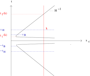
Figure 1: Space-time diagram (sketch) showing the evolution of a fixed comoving scale in our bouncing cosmology under the assumption that the bounce phase lies entirely within the Hagedorn phase. The vertical axis is time, the horizontal axis is comoving distance. The bounce time is chosen to be $t=0$. The Hagedorn phase corresponds to the time interval $-t_{H}<t<t_{H}$, the bounce phase is the interval $-t_{B}<t<t_{B}$. Outside of the bounce phase, the Hubble radius evolves as in a radiation phase of standard cosmology The black solid curve represents the Hubble radius $H^{-1}$. The red vertical line labelled by $k$ depicts a fixed comoving scale. This scale is smaller than the Hubble radius in the central region of the bounce, exits the Hubble radius at the time $t_{i}(k)$, and re-enters at a late time $t_{f}(k)$.

Let us recall the origin of the Hagedorn phase [6]: In the context of perturbative string theory, there is a maximal temperature $T_{H}$, the Hagedorn temperature [7], for a string gas in thermal equilibrium. As the universe contracts in our scenario, the temperature initially increases as in the usual radiation phase of standard cosmology. The energy is in the radiative degrees of freedom, the momentum modes of the strings. As the temperature approaches $T_{H}$, it becomes possible to excite the string oscillatory and winding mode degrees of freedom. In fact, close to the Hagedorn temperature, most of the energy in the string gas is contained in winding strings [28, 29].

The crucial point of the mechanism of [2] is the following: provided that our three large spatial dimensions are compact, the heat capacity $C_{V}$ of a gas of strings in thermal equilibrium scales as $r^{2}$ with the radius of the box. The heat capacity determines the root mean square mass fluctuations via

$$\langle\bigl{(}\delta M\bigr{)}^{2}\rangle\,=\,T^{2}C_{V}\,,$$ (3.17)

which then in turn induce metric perturbations. In longitudinal gauge (see e.g. [30, 31] for reviews of the theory of cosmological perturbations), and in the absence of anisotropic matter stress at late times, the metric takes the form

$$ds^{2}\,=\,-(1+2\Phi)dt^{2}+a(t)^{2}(1-2\Phi)d{\bf x}^{2}\,,$$ (3.18)

where $t$ is physical time, ${\bf x}$ are the comoving spatial coordinates of the three large spatial dimensions, $a(t)$ is the cosmological scale factor and $\Phi({\bf x},t)$ represents the fluctuation mode. On scales smaller than the Hubble radius, the metric fluctuations are driven by the matter fluctuations, on super-Hubble scales it is the metric fluctuations which are dominant since the matter oscillations have frozen out (thermal fluctuations cannot keep up with the Hubble expansion). Thus, to compute the late-time spectrum of metric fluctuations, the philosophy adopted in [2] (see also [32] for a corresponding treatment of fluctuations in inflationary cosmology and [33] for a discussion on the spectrum of thermal fluctuations corresponding to ordinary particles) is, for inhomogeneities on a fixed comoving scale, to follow the matter fluctuations until the scale exits the Hubble radius at time $t_{i}(k)$, and to use the Einstein constraint equations to determine the metric fluctuations at that time. The metric fluctuations will then be conserved on super-Hubble scales.

As long as the background dilaton velocity is negligible, the Einstein constraint equations (specifically, the relativistic Poisson equation)

$$\nabla^{2}\Phi\,=\,4\pi G\delta\rho\,,$$ (3.19)

(where $\rho$ is the energy density) then imply that the power spectrum of the metric fluctuation variable $\Phi$ is scale-invariant (for details on how to get from the spectrum of mass fluctuations to the power spectrum of $\Phi$ see [5]).

In order for (3.19) to apply, it is important that metric and matter fluctuations are related via the Einstein equations, and not e.g. via the dilaton gravity equations [12] (see [8] for a detailed discussion of this point). In our bouncing cosmology, the dilaton is taken to be constant throughout the evolution of the universe. Thus, there are no dilaton corrections to (3.19). We also note that the higher derivative corrections to (3.19) are suppressed by $(\nabla^{2}/M_{\ast}^{2})\sim(k/M_{\ast})^{2}$ (see [1] for a quantitative discussion). The comoving scales that we are interested in corresponds to the Hubble radius today, and one can easily check that this ratio is hugely suppressed (see section B for instance) in a non-inflationary scenario such as ours. In addition, the fact that there are no additional dynamical degrees of freedom compared to those in Einstein’s theory ensures that we need not worry about extra unstable (ghost like) or spurious excitations of the metric.

We are thus led to the following structure formation scenario: The universe begins in a cold contracting phase. The initial Hubble radius is set by the initial gas density, and it is natural to assume that the size of space is at least as large as the initial Hubble radius. If we begin the evolution at a temperature lower than the present radiation temperature, we are then ensured that the size of space at the bounce is sufficiently large to contain all fluctuation modes of current interest in cosmology . Local processes in at the beginning or during the course of the contraction phase establish thermal equilibrium over a scale which contains all fluctuation modes of interest to us. Matter remains homogeneous and isotropic throughout the bounce. In particular, during the Hagedorn phase of the bounce, we have a gas of strings. In the same way that a network of strings forming at a phase transition in a field theory model with cosmic strings [34] will contain strings of length larger than the Hubble radius (in particular, it will contain winding modes), after the transition to the Hagedorn phase, our gas of fundamental strings will contain winding modes, and it is the presence of these winding modes which are the key ingredient to obtain the form of the specific heat we are using. Thus, we are able to use the results of string thermodynamics to compute the spectrum of matter perturbations which then seed the scalar metric fluctuations.

3.2 Thermodynamics, a Brief Review

In order to compute the power spectrum of density fluctuations we have to compute the fluctuations in string energy, $\Delta E$, for these closed string modes inside an arbitrary volume $V$. Once we obtain $\Delta E(V)$, there is a well defined prescription on how to go over to the power spectrum ${\cal P}(k)$ as described in the next subsection. In order to obtain $\Delta E$ and eventually the power spectrum we have to understand the thermodynamics of the Hagedorn phase and here we start with a brief review of the same.

Specifically we are interested in a situation where we have $d=3$ large but compact spatial dimensions. The entropy $S$ of a string gas in thermal equilibrium in this background was derived in [11] (also see [2, 4]). During the Hagedorn phase, and in the case of a volume which is large in string units, the result is

$$S\,=\,{\cal E}+bv-{{\cal E}^{2d-1}\over(2d-1)!}\exp\left[-{c({\cal E}-kv)\over v^{2/3}}\right]\,,$$ (3.20)

where we have introduced the dimensionless variables

$${\cal E}\,\equiv\,{E\over T_{H}}\mbox{ and }v\,\equiv\,VT_{H}^{d}\,,$$ (3.21)

for convenience. $V$ is the volume of the $d$ large dimensions, and $b,c,k$ are ${\cal O}(1)$ constants (see [28, 2, 4]). This formula is valid in the regime ${\cal E}>kv$ (which is characteristic of the Hagedorn phase) and $v\gg v^{2/3}$ (which means that the volume of the universe is much larger than the string length).

Once we have the microcanonical entropy $S(E,V)$ as a function of the energy and the volume, it is straight forward to compute all the thermodynamic quantities. In particular we find that the inverse temperature $\beta$ is given by

$$\beta\,=\,{\partial S\over\partial E}$$ (3.22)

which implies

$${\beta\over\beta_{H}}\,=\,1+{c{\cal E}^{2d-1}\over(2d-1)!v^{2/3}}\exp\left[-{c({\cal E}-kv)\over v^{2/3}}\right]\,,$$ (3.23)

where we have used $v\ll{\cal E}$. Using the same approximation we find from (3.23) that the specific heat (or rather the heat capacity) is given by

$$C_{v}\,\equiv\,\beta_{H}\left({\partial{\cal E}\over\partial T}\right)_{v}\,=\,{(2d-1)!v^{2/3}\over cT(T_{H}-T)}\,,$$ (3.24)

which gives the characteristic scaling $C_{V}\sim r^{2}$ as a function of the radius of the volume which, by the discussion in the previous subsection implies a scale-invariant spectrum of metric fluctuations.

If the decrease in the Hubble radius at the end of the Hagedorn phase is not instantaneous, then the time $t_{i}(k)$ (and thus also the corresponding temperature $T(t_{i}(k))$ will depend on $k$. This will lead to a red tilt in the spectrum. In section (3.4) we will see that using (3.23) and (3.24) one can calculate the spectral tilt in the bouncing universe scenario quite precisely.

3.3 Spectrum of Perturbations

The dimensionless power spectrum of scalar metric fluctuations is defined by

$$P_{\Phi}(k)\,\equiv\,k^{3}|\Phi(k)|^{2}\,$$ (3.25)

where $\Phi(k)$ is the k’th Fourier mode of $\Phi(x)$, and we are using the convention of defining the Fourier transform of a function $f(x)$ including a factor of the square root of the volume of space.

Making use of the relativistic Poisson equation (3.19), (3.25) becomes

$$P_{\Phi}(k)\,=\,16\pi^{2}G^{2}k^{-1}|\delta\rho(k)|^{2}\,.$$ (3.26)

The Fourier space density perturbation of wavenumber $k$ can be determined from the mean square mass fluctuation $|\delta M|^{2}(r)$ in a sphere of radius $r(k)=k^{-1}$ via

$$|\delta\rho(k)|^{2}\,=\,k^{3}|\delta M|^{2}(r(k))\,,$$ (3.27)

and hence (3.25) becomes

$$P_{\Phi}(k)\,=\,16\pi^{2}G^{2}k^{2}(\delta M)^{2}(r(k))\,.$$ (3.28)

Plugging the expression (3.24) for the specific heat capacity of a string gas into (3.17) and then into (3.28) we finally obtain the following result for the power spectrum [2, 5]:

$$P_{\Phi}(k)\,=\,1920\pi^{2}c^{-1}G^{2}T_{H}^{4}\bigl{(}kr(k)\bigr{)}^{2}{T\over{T_{H}(1-T/T_{H})}}\,,$$ (3.29)

where for each value of $k$, the temperature $T$ is to be evaluated at the time that the mode $k$ exits the Hubble radius at time $t_{i}(k)$.

We see immediately that as a consequence of the specific stringy scaling of the heat capacity, we obtain a scale-invariant spectrum of fluctuations in the approximation when $T(t_{i}(k))$ is independent of $k$ as it will be if the Hubble radius drops abruptly. If the decrease of the scale factor is not instantaneous, then a small red tilt of the spectrum will be induced since smaller length scales exit the Hubble radius later, and the temperature then is smaller. We will come back to the issue of the magnitude of the spectral tilt shortly.

The overall amplitude of the spectrum is, as in [2, 5], determined by two factors, firstly the factor $G^{2}T_{H}^{2}$ which is the fourth power of the ratio of the Planck length and the string length, and secondly the final factor in (3.29) which depends on how close the temperature at the bounce point is to the Hagedorn temperature.

3.4 Spectral Tilt: General Formula

In this subsection we compute the spectral tilt $\eta_{s}-1$ which is defined by

$$P(k)\,\sim\,k^{\eta_{s}-1}\,.$$ (3.30)

To keep things general we do not specify the function $T=T(a)$. The spectral tilt can be calculated straightforwardly from (3.29). The key factor is the factor $1-T/T_{H}$ in the denominator of the expression. This is the term that carries the dominant dependence on $k$. The reason is that at all times $t_{i}(k)$, the temperature is very close to the Hagedorn temperature so that the only other factor which depends on $k$, namely the factor $T$ in the numerator of (3.29) can be taken to be constant. From (3.29)

$$\ln{\cal P}\,=\,\ln C-\ln(1-T/T_{H})\,,$$ (3.31)

where the constant $C$ stands for the product of all terms in (3.29) which do not depend on $k$. Hence,

$${d\ln{\cal P}\over dk}\,=\,{d\ln{\cal P}\over da}{da\over dk}\,,$$ (3.32)

where the comoving wave-vector $k$ exits the Hubble radius when the scale factor $a$ is given by

$$k\,=\,Ha\,=\,\dot{a}$$ (3.33)

which implies

$$\dot{k}\,=\,\ddot{a}\,.$$ (3.34)

Note that (3.33) determines $k$ as a function of the scale factor $a$, and through its dependence on time, also as a function of time, $k=k(a)=k(a(t))$.

From (3.33) we find

$${da\over dk}\,=\,\left({da\over dt}\right)/{dk\over dt}\,=\,{\dot{a}\over\ddot{a}}\,.$$ (3.35)

Thus,

$${d\ln{\cal P}\over dk}\,=\,{d\ln{\cal P}\over da}{\dot{a}\over\ddot{a}}\,.$$ (3.36)

Now, straightforwardly one finds

$${d\ln{\cal P}\over da}\,=\,{T^{\prime}T_{H}\over(T_{H}-T)T}\,,$$ (3.37)

where ^′ denotes the differentiation with respect to the scale factor. Putting all the things together we have

$${d\ln{\cal P}\over dk}\,=\,{\dot{a}\over\ddot{a}}{T^{\prime}T_{H}\over(T_{H}-T)T}\,,$$ (3.38)

and, finally,

$$\eta_{s}-1\,\equiv\,{d\ln{\cal P}\over d\ln k}\,=\,k{d\ln{\cal P}\over dk}\,=\,{\dot{a}^{2}\over\ddot{a}}{T^{\prime}T_{H}\over(T_{H}-T)T}$$ (3.39)

This is a general result which holds for any $T(a)$ and $a(t)$. One can further simplify (3.39) using the following redefinition:

$$a(t)\,=\,e^{{\cal N}(t)}$$ (3.40)

One can check that the expression for the spectral tilt then reduces to

$$\eta_{s}-1\,=\,\left[{H^{2}\over H^{2}+\dot{H}}\right]\left[{1\over T}{dT\over d{\cal N}}{T_{H}\over(T_{H}-T)}\right]\,\equiv\,XY\,,$$ (3.41)

where $X(Y)$ denotes the term in the first (second) set of brackets. Note that while the first term depends on how the scale factor evolves with time, the second term primarily depends on how the temperature changes with the expansion of the universe, $T({\cal N})$.

3.5 Spectral Tilt and Amplitude during Bounce

In this section we evaluate the magnitude of the spectral tilt in our scenario keeping in mind the various consistency requirements of the mechanism and the fact that we have to reproduce the correct amplitude of fluctuation in CMB. We recall that, as in inflationary cosmology, the cosmological fluctuations on a fixed comoving scale $k$ freeze out at the time $t_{i}(k)$ when their wavelength crosses the Hubble radius. This is similar to what happens in the case of cosmological inflation. However, whereas in inflationary cosmology physical scales are increasing exponentially while the Hubble radius stays approximately constant, and thus scales are “expelled” from the Hubble volume, in a bouncing scenario such as the one presented in this paper, scales exit the Hubble radius in spite of the fact that during the relevant time interval the universe (and hence the physical scales) expands very little. Instead, the Hubble radius sharply decreases to a microscopic value starting from infinity (at the bounce point).

Since the scale of the bounce is governed by $\lambda\sim M_{\ast}$ which is expected to be of the order of the string scale, approximately in a string time the Hubble radius decreases to string length from infinity. All the scales which we observe today exit the Hubble radius in the process .

Let us first compute the temperature dependent factor $Y$ in the equation (3.41) for the spectral tilt. As we will soon see phenomenological constraints will tell us that the bounce has to occur just after the onset of the Hagedorn phase when the background evolution is still governed by radiation (massless modes) as explained in the appendix B. The task of computing $Y$ is then easy as the temperature is just given by

$$T\,=\,T_{b}e^{-{\cal N}}\approx T_{H}e^{-{\cal N}}\,.$$ (3.42)

Hence,

$$Y\,=\,{T_{H}\over T_{H}-T}\,\approx\,{T_{H}\over T_{H}-T_{b}}\,,$$ (3.43)

since all the relevant modes are effectively expelled out of the Hubble radius very near to the bounce point.

For (2.7) one can easily compute the first term, $X$, in the expression of the spectral tilt (3.41), obtaining

$$X\,\equiv\,{H^{2}\over H^{2}+\dot{H}}\,=\,{\tanh^{2}(\lambda t/\sqrt{2})\over\tanh^{2}(\lambda t/\sqrt{2})+\mathtt{sech}^{2}(\lambda t/\sqrt{2})}\approx{\lambda^{2}t^{2}\over 2+{\cal O}(\lambda^{4}t^{4})}\,.$$ (3.44)

Putting everything together, we have a rather simple expression for the spectral tilt evaluated at a length scale given by the comoving wavenumber $k$ (note that the tilt in general is scale-dependent)

$$\eta_{s}-1\,=\,-{\lambda^{2}t_{k}^{2}\over 2}{T_{H}\over T_{H}-T_{b}}\,\equiv\,-{\lambda^{2}t_{k}^{2}\over 2}{T_{H}\over\Delta T}$$ (3.45)

and we recall that the physical wavelength of the mode exits the Hubble radius at a time denoted by $t_{i}(k)$.

We will soon find out that for the physical scales that we observe in the CMB, $t_{i}(k)<<\lambda^{-1}$. In this approximation $t_{i}(k)$ is determined by:

$$k\,=\,Ha\,=\,\dot{a}\,=\,{\lambda\over\sqrt{2}}\sinh{\lambda t\over\sqrt{2}}\approx{\lambda^{2}t_{i}(k)\over 2}$$ (3.46)

so that

$$\eta_{s}-1\,\approx\,-\lambda^{2}t_{k}^{2}{T_{H}\over\Delta T}\,=\,-2\left({k\over\lambda}\right)^{2}{T_{H}\over\Delta T}$$ (3.47)

The comoving wave number corresponding to the Hubble radius today is given by

$$k_{0}\,=\,H_{0}a_{0}\,,$$ (3.48)

and thus we have

$$\eta_{s}-1\,=\,-2\left({H_{0}a_{0}\over\lambda}\right)^{2}{T_{H}\over\Delta T}$$ (3.49)

Since during the bounce phase the universe expands very little, one can easily estimate $a_{0}\sim T_{0}/T_{H}$ using the usual scaling during radiation era. Then it is easy to check that (see also appendix B)

$$|\eta_{s}-1|\approx 10^{-60}\left({M_{s}\over\lambda}\right)^{2}{T_{H}\over\Delta T}$$ (3.50)

Thus we observe that the “bounce factor” $X$ is typically very small and thus, as long as the temperature dependent factor $Y$ is not too large we will reproduce a scale-invariant spectrum.

For illustration let us consider a specific example which is consistent with all the requirements, viz. (i) we get a scale invariant spectrum, (ii) amplitude of fluctuation $\sim 10^{-10}$ as required by CMB, (iii) bounce occurs near the transition, i.e. $\rho_{b}\sim M_{s}^{2}\sim M_{p}^{2}\lambda^{2}$, and finally (iv) the fluctuations in energy are dominated by the closed strings in the Hagedorn phase. As explained in the appendix, the last constraint is met as long as

$${\Delta T\over T_{H}}<10^{-30}$$ (3.51)

We will consider the limiting case, when $\Delta T/T_{H}\sim 10^{-30}$. Now the amplitude of fluctuation is approximately given by

$$\delta_{\mathtt{CMB}}^{2}\sim 10^{-10}\sim\left({M_{s}\over M_{p}}\right)^{4}{T_{H}\over\Delta T}\Rightarrow M_{s}\sim 10^{-10}M_{p}$$ (3.52)

In other words an $M_{s}\sim 10^{-10}M_{p}$, reproduces the required amplitude of perturbations observed in CMB. Requirement (ii) now forces $\lambda\sim 10^{-10}M_{s}$ giving rise to a very small red spectral tilt

$$|\eta_{s}-1|\sim 10^{-10}$$ (3.53)

This situation can of course change once we include additional corrections to the entropy relation, $S({\cal E},v)$ near the transition, or if the scales involved are different. In fact, a really interesting case emerges if one considers the string scale to be around ($Tev$) which is also interesting from the point of view of particle physics phenomenology. In this case, $\lambda\sim 10^{-15}M_{s}\sim 10^{-30}M_{p}$, and one obtains a spectral tilt which is just becoming observationally significant!

Before ending this section let us point out why for the phenomenological success, we require the bounce to occur close to the transition. If $\Delta T/T_{H}\ll 10^{-30}$, for instance, then in order to get the amplitude of spectrum right, one has consider an unacceptably low string scale. Typically, deep inside the Hagedorn phase $\Delta T/T_{H}$ is indeed very small, it is suppressed by an exponential of an exponential, and thus is not phenomenologically viable.

4 Conclusions and Discussion

In this paper we have extended the non-singular bouncing cosmology construction obtained in [1] to more general matter sources, including a gas of closed strings. We have shown that this model leads to a simple implementation of the string gas structure formation mechanism proposed in [2], provided that the energy density at the bounce is sufficiently large to lead a Hagedorn phase of the string gas, and the three large spatial dimensions are compact.

The higher derivative gravity model discovered in [1] is distinguished by being free of ghosts. No new gravitational degrees of freedom appear compared to those of Einstein gravity. The dilaton can be consistently taken to be frozen at all times. Thus, it is reasonable to assume that the metric fluctuations can be described using the equations of general relativistic perturbation theory.

In this case, all of the conditions to obtain a scale-invariant spectrum of scalar metric fluctuations detailed in [5, 8] are satisfied. The matter fluctuations in the Hagedorn phase around the bounce time, when the Hubble radius diverges, are characterized by a heat capacity $C_{V}$ which scales as $r^{2}$ with the size of the region [11, 2, 4]. Via the relativistic Poisson equation, these matter fluctuations induce a scale-invariant spectrum of metric fluctuations which propagate to late times. being squeezed, but without modification of the spectral shape. The spectrum has a red tilt, like in the string gas cosmology scenario [2, 5]. However, the magnitude of the tilt - calculated in this paper - is very small.

Assuming that the initial state is chosen very early in the contracting phase, when the matter density is smaller than the current density, and assuming that the spatial size is at least one Hubble volume at that time, we obtain a cosmology which resolves the horizon and entropy problems of standard cosmology . Thermal equilibrium over large distances is established in the contracting phase, thus allowing us to use equilibrium thermodynamics of strings in the Hagedorn phase, even if the latter is of a duration short compared to the physical length at the bounce time of perturbations relevant to current cosmology. Thus, our model provides an explicit toy model which demonstrates, in the context of an explicit action for the background space-time, that all the criteria required to obtain a scale-invariant spectrum in the scenario of [2] can be realized, and thus successfully addressed the concerns raised in [9].

Appendix A Exact and Approximate Bounce Solutions

In the previous work [1], the presence of a cosmological constant was required for the late-time consistency of the ansatz (2.7) for the solution. To see this consider the behavior at large times. It is clear that the scale factor tends to a de Sitter solution:

$$a(t)\,\rightarrow\,{1\over 2}e^{\sqrt{w\over 2}\ t}\,,$$ (A.54)

while one can check that all the higher curvature terms vanish:

$$\widetilde{G}_{00}^{HD}\,\equiv\,\sum_{n=0}^{\infty}\widetilde{G}_{00}^{n}\rightarrow\mathtt{sech}^{2}\left(\sqrt{w\over 2}\ t\right)\rightarrow 0\,.$$ (A.55)

As a result, we are just left with Einstein’s theory of gravity. In the absence of the cosmological constant, at large times when the higher derivative corrections become small, we will instead make a transition to the usual radiation dominated era of Einstein gravity.

For the cosine hyperbolic ansatz the modified Einstein tensor looks like

$$\widetilde{G}_{00}\, = \,L_{0}+L_{2}\mathtt{sech}^{2}\left(\lambda t/\sqrt{2}\right)+L_{4}\mathtt{sech}^{4}\left(\lambda t/\sqrt{2}\right)+L_{6}\mathtt{sech}^{6}\left(\lambda t/\sqrt{2}\right)$$ (A.56)

$$= \,C_{0}+C_{2}\lambda^{2}t^{2}+C_{4}\lambda^{4}t^{4}+{\cal O}(\lambda^{6}t^{6})\,,$$ (A.57)

where the $L$’s are given in terms of the function $\Gamma$ by

$$L_{0}(\lambda^{2})\, = \,{3\lambda^{2}\over 2}\,,$$ (A.58)

$$L_{2}(\lambda^{2})\, = \,{9\lambda^{2}\over 2}\left[1-\Gamma(\lambda^{2})-4{c_{0}\over M^{2}}\lambda^{2}\right]-{3\lambda^{2}\over 2}\,,$$ (A.59)

$$L_{4}(\lambda^{2}) = {9\lambda^{2}\over 2}\left[2{c_{0}\over M^{2}}\lambda^{2}+{5\over 6}\Gamma^{\prime}(\lambda^{2})\lambda^{2}\right]\,,$$ (A.60)

$$L_{6}(\lambda^{2})\, = \,{9\lambda^{2}\over 2}\left[\Gamma(\lambda^{2})-1-\Gamma^{\prime}(\lambda^{2})\lambda^{2}\right]\,,$$ (A.61)

and the $C$’s can be read off from $L$’s:

$$C_{0}\, = \,L_{0}+L_{2}+L_{4}+L_{6}\,,$$ (A.62)

$$C_{2}\, = \,-\frac{1}{2}\left(L_{2}+2L_{4}+3L_{6}\right)\,,$$ (A.63)

$$C_{4}\, = \,{1\over 16}\left(L_{2}+6L_{4}+15L_{6}\right)\,,$$ (A.64)

and now we can match them with the coefficients coming from the stress energy tensor.

Near the bounce point ($t=0$ and $a=1$ by convention), we can expand the function $\rho(t)$ in a Taylor series:

$$\rho(t)\,=\,\left.\rho\right|_{t=0}+\left.{d\rho\over dt}\right|_{t=0}t+\left.{1\over 2}{d^{2}\rho\over dt^{2}}\right|_{t=0}t^{2}+\left.{1\over 6}{d^{3}\rho\over dt^{3}}\right|_{t=0}t^{3}+\left.{1\over 24}{d^{4}\rho\over dt^{4}}\right|_{t=0}t^{4}+\dots$$ (A.65)

The terms with odd powers of $t$ vanish by our assumption of a symmetric bounce with bounce point $t=0$. Replacing time derivatives by derivatives with respect to the scale factor, we obtain

$$\rho(t)\,\approx\,\left.\rho\right|_{a=1}+\left.{\lambda^{2}t^{2}\over 4}{d\rho\over da}\right|_{a=1}+\left.{\lambda^{4}t^{4}\over 96}\left({d\rho\over da}\right|_{a=1}+\left.3{d^{2}\rho\over da^{2}}\right|_{a=1}\right)\,,$$ (A.66)

where we have used the specific ansatz (2.7).

Thus, by matching the $C$ ’s in (A.57) with the coefficients of the stress energy tensor (A.66), we essentially have three equations which determine the two dynamical quantities, $\rho_{b},\lambda$ along with giving us a constraint. One can check that the exact solutions that were found in [1] in the presence of a cosmological constant and radiation is a subset of the approximate solutions described above.

In the case when one can apply the ideal fluid approximation (2.9), the equations simplify considerably and one obtains

$$-{3\lambda^{2}(12{c_{0}\over M^{2}}\lambda^{2}+\Gamma^{\prime}\lambda^{2})\over 8}\,=\,{2\lambda^{2}\left[6\Gamma-7-4\Gamma^{\prime}\lambda^{2}\right]\over 1+\omega}\,=\,{48\lambda^{2}\left[42\Gamma-43-30\Gamma^{\prime}\lambda^{2}+24c_{0}\lambda^{2}\right]\over(1+\omega)(9\omega+11)}\,=\,{\rho_{b}\over M_{p}^{2}}\,.$$ (A.67)

determining $\lambda^{2},\rho_{b}$ and giving rise to an additional constraint. One can rewrite the above equations in a more illuminating form:

$${\cal K}\left({\lambda^{2}\over M_{\ast}^{2}}\right)=0$$

$$1+\omega\,=\,{16{\cal F}({\lambda^{2}\over M_{\ast}^{2}})\over 3\lambda^{2}{\cal G}\left({\lambda^{2}\over M_{\ast}^{2}}\right)}$$

and

$$\rho_{b}\,=\,{3M_{p}^{2}\lambda^{2}{\cal G}({\lambda^{2}\over M_{\ast}^{2}})\over 8}\,$$

where we have defined dimensionless functions:

$${\cal F}\left({\lambda^{2}\over M_{\ast}^{2}}\right)\equiv 6\Gamma-7-4\Gamma^{\prime}\lambda^{2}$$ (A.68)

$${\cal G}\left({\lambda^{2}\over M_{\ast}^{2}}\right)\equiv-\left(12{c_{0}\lambda^{2}\over M^{2}}+\lambda^{2}\Gamma^{\prime}\right)$$ (A.69)

and

$${\cal K}\left({\lambda^{2}\over M_{\ast}^{2}}\right)\equiv{942\Gamma-955-676\Gamma^{\prime}\lambda^{2}+576{c_{0}\lambda^{2}\over M^{2}}\over 36{c_{0}\lambda^{2}\over M^{2}}-61\Gamma^{\prime}\lambda^{2}+96\Gamma-112}-3{{\cal F}\left({\lambda^{2}\over M_{\ast}^{2}}\right)\over{\cal G}\left({\lambda^{2}\over M_{\ast}^{2}}\right)}\,$$ (A.70)

A few comments are now in order. Since we want to restrict ourselves only to matter sources which are “consistent” (for instance ghost-free), they have to satisfy the dominant energy condition. This, in particular, implies

$$\rho(1)\,>\,0\mbox{ and }\left.{d\rho\over da}\right|_{a=1}\,<\,0\,\Longleftrightarrow-1\leq\omega\leq 1$$ (A.71)

imposing crucial restrictions on when one can have such a bounce and therefore prevent the singularity. Specifically, it says that the dimensionless functions that we introduced, viz. ${\cal F,\ G,\ K}$, has to be positive at the solution point.

One may also wonder why we need to keep track of terms up to ${\cal O}(t^{4})$. Naively, one would expect that matching terms up to ${\cal O}(t^{2})$ should be sufficient to capture the physics near the bounce. We should remember that, for consistency, we need to solve the full Einstein equations, i.e. $\widetilde{G}_{mn}=T_{mn}$ up to ${\cal O}(t^{2})$. In terms of the “Hubble equation” (2.5) this is equivalent to looking at terms up to ${\cal O}(t^{4})$.

Appendix B Modeling the transition from Hagedorn to Radiation

We have seen in our analysis that for phenomenological success of the model, the bounce point should occur when string scale energy density is reached, i.e. right around the time when the massive modes are being excited and we are entering (or just entered the Hagedorn phase). In fact this is also important for the consistency of our computations of the perturbation spectrum, as we now illustrate. In order to be able to do any kind of “local” analysis with the metric fluctuations it is imperative that we are able to define a local matter density function, $\rho(x)$, which is sourcing the metric. Now this is possible if the following limit is well defined:

$$\rho(x)\,=\,\lim_{r\rightarrow 0}{M_{r}\over V_{r}}\,,$$ (B.72)

where $M_{r}$ and $V_{r}$ are the mass/energy and volume respectively inside a sphere of radius $r$ around the point $x$. It is clear that a non-trivial and a well-defined limit only exists iff $M_{r}\sim r^{3}$ which is indeed the case for ordinary particles. However in the Hagedorn phase $E\sim r^{2}$ and therefore the density function is ill defined and accordingly one cannot proceed to obtain its Fourier transform or power spectrum for that matter. Thus in order for us to perform the usual density perturbation analysis it is imperative that for the distance scales that are relevant for CMB, the energy is still dominated by the contribution from the massless modes which would give rise to an $r^{3}$ term.

Now, in order to check whether this is true one would need to compare the energy in the massive string modes (Hagedorn matter) given by (3.23)

$$E_{\mathtt{massive}}\,=\,c_{\mathtt{hag}}r^{2}M_{s}^{3}\left\{\ln\left[{T\over 1-T/T_{H}}\right]+\log\log\mbox{ terms}\right\}$$ (B.73)

with that of radiation (massless modes)

$$E_{\mathtt{rad}}\,=\,c_{\mathtt{rad}}T^{4}r^{3}$$ (B.74)

inside spheres of the relevant scales. Here $c_{\mathtt{rad}},c_{\mathtt{hag}}\sim{\cal O}(1)$ constants. Now, in order for the limit (B.72) to exist, minimally we require

$$\zeta_{E}\,\equiv\,{E_{\mathtt{rad}}\over E_{\mathtt{massive}}}\,\sim\,\left({T\over M_{s}}\right)^{4}{M_{s}r_{0}\over\ln\left[{T\over 1-T/T_{H}}\right]}\,>\,1\,,$$ (B.75)

where $r_{0}$ is the physical scale at the time of the bounce corresponding to the Hubble radius today. Therefore as long as the logarithm in the denominator $\sim{\cal O}(1)$, since at the time of the bounce $T\sim M_{s}$, to satisfy (B.75) we simply require

$$\zeta_{E}\,\sim\,M_{s}r_{0}\,>\,1\,.$$ (B.76)

It is easy to estimate this quantity. We know that during the bounce the universe expands very little. Therefore, making the simplifying assumption that most of the expansion of our universe occurred during the radiation era since string scale energy density, we have

$${r_{0}\over H_{0}^{-1}}\,=\,{T_{0}\over M_{s}}\Rightarrow M_{s}r_{0}\,\sim\,{M_{p}\over T_{0}}\sim 10^{30}\,\gg\,1\,.$$ (B.77)

Indeed, (B.75) is easily satisfied for the relevant scales that we are observing in CMB today and therefore our analysis of perturbation spectrum is well justified. As an aside, we notice that for all scales $r>r_{0}$ the energy is going to be dominated by radiation and in particular the evolution of our universe would also be governed by radiation.

What now becomes crucial is to verify that it is still the massive string modes of the Hagedorn phase that dominate the energy fluctuations in a sphere of radius $r_{0}$, and not the massless modes. The amplitudes of fluctuation is proportional to the respective specific heats (more precisely the heat capacities) and therefore in order for the power spectrum (3.29) to hold we need

$$\zeta_{C}\,\equiv\,{C_{\mathtt{rad}}\over C_{\mathtt{massive}}}\,<\,1$$ (B.78)

Differentiating the expressions for the energies with respect to temperature for the respective phases we have

$$\zeta_{C}\,=\,r_{0}M_{s}\bigl{(}1-{T\over{T_{H}}}\bigr{)}\,.$$ (B.79)

Thus, in order to satisfy (B.78) one requires

$${\Delta T\over T_{H}}\,\equiv\,1-{T\over T_{H}}\,<\,10^{-30}\,.$$ (B.80)

Appendix C Including the Dilaton and Other Light Moduli Fields

So far we have not discussed the possible role of moduli fields, such as the dilaton or radion that are present in any string theory compactifications. It is well-known that for consistency of late time physics (fifth force constraints, and bounds on variation of physical constants) one typically requires that these moduli fields are stabilized at a scale which is at least higher than the scale of big bang nucleosynthesis, i.e. Mev. There are two different possibilities that are compatible with our scenario. (i) If the scale of stabilization is higher than the string scale, then the bounce never probes this regime and the moduli fields always remain frozen playing no role either in the background evolution or in the generation of fluctuations. (ii) A second possibility, that the moduli are stabilized at a scale much lower than the string scale where all the dynamics is taking place is also consistent with our scenario. Let us look at this more carefully.

In the Einstein frame, the action for these scalars just looks like a free theory

$$S_{\phi}\,=\,-\frac{1}{2}\int d^{4}x\sqrt{-g}(\partial\phi)^{2}\,,$$ (C.81)

where $\phi$ has been appropriately normalized. An important subtlety is that after the conformal transformation (i.e. in the Einstein frame) the moduli fields such as the dilaton couple to the massive string modes. Thus, if there is stringy Hagedorn matter (massive closed string modes) present, then such matter would typically source the dilaton. However, as we explained before, we are primarily interested in a scenario where the energy density is not yet dominated by Hagedorn matter (only the fluctuations are) and in fact its energy density is hugely suppressed as compared to radiation. Therefore, such a source term can be completely ignored. In this context we note that since radiation is conformal, it does not yield any coupling to the dilaton after the conformal transformation. Let us therefore investigate the evolution of the free theory (C.81).

Once we include the dilaton, the generalized Einstein equation reads

$$\widetilde{G}_{00}\,=\,{1\over M_{p}^{2}}(\rho_{\mathtt{rad}}+\rho_{\phi})$$ (C.82)

where

$$\rho_{\phi}\,=\,{\dot{\phi}^{2}\over 2}\,.$$ (C.83)

This has to be supplemented by the dilaton equation

$$\ddot{\phi}+3H\dot{\phi}\,=\,0\,.$$ (C.84)

One can solve these equations. For instance, the dilaton equation yields

$$\rho_{\phi}\,=\,{\dot{\phi}^{2}\over 2}=\rho_{\phi,b}a^{-6}\,.$$ (C.85)

Using the specific bounce solution we find

$$\phi(t)\,=\,\phi_{b}+\sqrt{\rho_{\phi,b}\over M_{p}^{2}\lambda^{2}}\left[\tanh(t\sqrt{\lambda/2})\mathtt{sech}(t\sqrt{\lambda/2})+2\tan^{-1}(e^{t\sqrt{\lambda/2}})-{\pi\over 2}\right]\,.$$ (C.86)

It is interesting to note that during the course of the bounce $\phi$ changes only by a finite amount:

$$\Delta\phi\equiv\phi(\infty)-\phi(-\infty)\,=\,\pi\sqrt{\rho_{\phi,b}\over M_{p}^{2}\lambda^{2}}\,.$$ (C.87)

Thus, we observe that if

$${\rho_{\phi,b}\over M_{p}^{2}\lambda^{2}}\,\ll\,1\,,$$ (C.88)

the string coupling

$$g_{s}\,\sim\,e^{\phi/M_{p}}$$ (C.89)

changes very little. Moreover, since the kinetic energy of the dilaton is small, it does not effect the evolution of the metric. In particular, it is completely consistent to set the value of $\phi$ to be a constant.

References

- [1] T. Biswas, A. Mazumdar and W. Siegel, “Bouncing universes in string-inspired gravity,” JCAP 0603, 009 (2006) [arXiv:hep-th/0508194].
- [2] A. Nayeri, R. H. Brandenberger and C. Vafa, “Producing a scale-invariant spectrum of perturbations in a Hagedorn phase of string cosmology,” arXiv:hep-th/0511140.
- [3] R. H. Brandenberger, A. Nayeri, S. P. Patil and C. Vafa, “String gas cosmology and structure formation,” arXiv:hep-th/0608121.
- [4] A. Nayeri, “Inflation free, stringy generation of scale-invariant cosmological fluctuations in D = 3 + 1 dimensions,” arXiv:hep-th/0607073.
- [5] R. H. Brandenberger, A. Nayeri, S. P. Patil and C. Vafa, “String gas cosmology and structure formation,” arXiv:hep-th/0608121.
- [6] R. H. Brandenberger and C. Vafa, “Superstrings In The Early Universe,” Nucl. Phys. B 316, 391 (1989).
- [7] R. Hagedorn, “Statistical Thermodynamics Of Strong Interactions At High-Energies,” Nuovo Cim. Suppl. 3, 147 (1965).
- [8] R. H. Brandenberger et al., “More on the spectrum of perturbations in string gas cosmology,” arXiv:hep-th/0608186.
- [9] N. Kaloper, L. Kofman, A. Linde and V. Mukhanov, “On the new string theory inspired mechanism of generation of cosmological perturbations,” arXiv:hep-th/0608200.
- [10] R. Danos, A. R. Frey and A. Mazumdar, Phys. Rev. D 70, 106010 (2004) [arXiv:hep-th/0409162].
- [11] N. Deo, S. Jain, O. Narayan and C. I. Tan, “The Effect of topology on the thermodynamic limit for a string gas,” Phys. Rev. D 45, 3641 (1992).
- [12] A. A. Tseytlin and C. Vafa, “Elements of string cosmology,” Nucl. Phys. B 372, 443 (1992) [arXiv:hep-th/9109048].
- [13] G. Veneziano, “Scale Factor Duality For Classical And Quantum Strings,” Phys. Lett. B 265, 287 (1991).
-
[14]
D. J. Gross and E. Witten,
“Superstring Modifications Of Einstein’s Equations,”
Nucl. Phys. B 277, 1 (1986);
A. A. Tseytlin, “Ambiguity in the Effective Action in String Theories,” Phys. Lett. B 176, 92 (1986). - [15] B. Zwiebach, “Curvature Squared Terms And String Theories,” Phys. Lett. B 156, 315 (1985).
-
[16]
P. Van Nieuwenhuizen,
“On Ghost-Free Tensor Lagrangians And Linearized Gravitation,”
Nucl. Phys. B 60, 478 (1973);
A. Nunez and S. Solganik, “Ghost constraints on modified gravity,” Phys. Lett. B 608, 189 (2005) [arXiv:hep-th/0411102];
T. Chiba, “Generalized gravity and ghost,” JCAP 0503, 008 (2005) [arXiv:gr-qc/0502070]. - [17] G. Calcagni, B. de Carlos and A. De Felice, “Ghost conditions for Gauss-Bonnet cosmologies,” Nucl. Phys. B 752, 404 (2006) [arXiv:hep-th/0604201].
- [18] N. Moeller and B. Zwiebach, “Dynamics with infinitely many time derivatives and rolling tachyons,” JHEP 0210, 034 (2002) [arXiv:hep-th/0207107].
- [19] T. Biswas, M. Grisaru and W. Siegel, “Linear Regge trajectories from worldsheet lattice parton field theory,” Nucl. Phys. B 708, 317 (2005) [arXiv:hep-th/0409089].
- [20] W. Siegel, “Stringy gravity at short distances,” arXiv:hep-th/0309093.
-
[21]
S. Mandelstam,
“Interacting String Picture of Dual Resonance Models,”
Nucl. Phys. B 64, 205 (1973);
M. Kaku and K. Kikkawa, “The Field Theory Of Relativistic Strings, Pt. 1: Trees,” Phys. Rev. D 10, 1110 (1974);
M. Kaku, “The Field Theory Of Spinning Strings,” Phys. Rev. D 10, 3943 (1974);
M. Kaku and K. Kikkawa, “The Field Theory Of Relativistic Strings. Pt. 2: Loops And Pomerons,” Phys. Rev. D 10, 1823 (1974);
E. Cremmer and J. L. Gervais, “Combining And Splitting Relativistic Strings,” Nucl. Phys. B 76, 209 (1974);
E. Cremmer and J. L. Gervais, “Infinite Component Field Theory Of Interacting Relativistic Strings And Dual Theory,” Nucl. Phys. B 90, 410 (1975);
M. B. Green and J. H. Schwarz, “Superstring Field Theory,” Nucl. Phys. B 243, 475 (1984);
E. Witten, “Noncommutative Geometry And String Field Theory,” Nucl. Phys. B 268, 253 (1986);
D. J. Gross and A. Jevicki, “Operator Formulation of Interacting String Field Theory,” Nucl. Phys. B 283, 1 (1987);
Z. Hlousek and A. Jevicki, “Bose-Fermi Equivalence In Witten’s Interacting String Field Theory,” Nucl. Phys. B 288, 131 (1987);
D. J. Gross and A. Jevicki, “Operator Formulation Of Interacting String Field Theory. 2,” Nucl. Phys. B 287, 225 (1987);
E. Cremmer, A. Schwimmer and C. B. Thorn, “The Vertex Function in Witten’s Formulation of String Field Theory,” Phys. Lett. B 179, 57 (1986). -
[22]
D. Evens, J. W. Moffat, G. Kleppe and R. P. Woodard,
“Nonlocal Regularizations Of Gauge Theories,”
user
/Subtype /Link
/Border [ 0 0 0 ]
/A ¡¡ /S /URI /URI (http://www-spires.slac.stanford.edu/spires/find/hep/www?j=PHRVA%2CD43%2C499) ¿¿Phys. Rev. D 43 (1991) 499;
A. A. Tseytlin, “On singularities of spherically symmetric backgrounds in string theory,” Phys. Lett. B 363, 223 (1995) [arXiv:hep-th/9509050]. - [23] M. Borunda and L. Boubekeur, “The effect of alpha’ corrections in string gas cosmology,” arXiv:hep-th/0604085.
-
[24]
S. Weinberg, Critical phenomena for field theorists, in Understanding the fundamental
constituents of matter, proc. of the International School of Subnuclear Physics, Erice,
1976, ed. A. Zichichi (Plenum, New York, 1978) p. 1;
Ultraviolet divergences in quantum theories of gravitation, in General relativity: an Einstein centenary survey, eds. S.W. Hawking and W. Israel (Cambridge University, Cambridge, 1979) p. 790. - [25] R. P. Woodard, “Avoiding dark energy with 1/R modifications of gravity,” arXiv:astro-ph/0601672.
- [26] H. J. Schmidt, “Variational derivatives of arbitrarily high order and multiinflation cosmological models,” Class. Quant. Grav. 7, 1023 (1990).
- [27] R. Brandenberger and N. Shuhmaher, “The confining heterotic brane gas: A non-inflationary solution to the entropy and horizon problems of standard cosmology,” JHEP 0601, 074 (2006) [arXiv:hep-th/0511299].
- [28] N. Deo, S. Jain and C. I. Tan, “String Statistical Mechanics Above Hagedorn Energy Density,” Phys. Rev. D 40, 2626 (1989).
- [29] D. Mitchell and N. Turok, “Statistical Properties of Cosmic Strings,” Nucl. Phys. B 294, 1138 (1987).
- [30] V. F. Mukhanov, H. A. Feldman and R. H. Brandenberger, “Theory Of Cosmological Perturbations. Part 1. Classical Perturbations. Part 2. Quantum Theory Of Perturbations. Part 3. Extensions,” Phys. Rept. 215, 203 (1992).
- [31] R. H. Brandenberger, “Lectures on the theory of cosmological perturbations,” Lect. Notes Phys. 646, 127 (2004) [arXiv:hep-th/0306071].
- [32] R. H. Brandenberger and R. Kahn, “Cosmological Perturbations In Inflationary Universe Models,” Phys. Rev. D 29, 2172 (1984).
- [33] J. Magueijo and L. Pogosian, “Could thermal fluctuations seed cosmic structure?,” Phys. Rev. D 67, 043518 (2003) [arXiv:astro-ph/0211337].
-
[34]
A. Vilenkin and E.P.S. Shellard, “Cosmic Strings and Other
Topological Defects,” (Cambridge Univ. Press, Cambridge, 1994);
M. B. Hindmarsh and T. W. B. Kibble, “Cosmic strings,” Rept. Prog. Phys. 58, 477 (1995) [arXiv:hep-ph/9411342];
R. H. Brandenberger, “Topological defects and structure formation,” Int. J. Mod. Phys. A 9, 2117 (1994) [arXiv:astro-ph/9310041]. -
[35]
T. Biswas and A. Mazumdar,
“Can we have a stringy origin behind Omega(Lambda)(t) infinity
Omega(m)(t)?,”
arXiv:hep-th/0408026;
“A stringy origin of the recent acceleration,” Phys. Lett. B 634, 437 (2006). T. Biswas, R. Brandenberger, A. Mazumdar and T. Multamaki, “Current acceleration from dilaton and stringy cold dark matter,” Phys. Rev. D 74, 063501 (2006) [arXiv:hep-th/0507199].