Abstract

As an extension of holography with flavour, we analyze in detail the embedding of a $\text{D}7$-brane probe into the Polchinski-Strassler gravity background, in which the breaking of conformal symmetry is induced by a $3$-form flux $G_{3}$. This corresponds to giving masses to the adjoint chiral multiplets. We consider the ${\cal N}=2$ supersymmetric case in which one of the adjoint chiral multiplets is kept massless while the masses of the other two are equal. This setup requires a generalization of the known expressions for the backreaction of $G_{3}$ in the case of three equal masses to generic mass values. We work to second order in the masses to obtain the embedding of $\text{D}7$-brane probes in the background. At this order, the $2$-form potentials corresponding to the background flux induce an $8$-form potential which couples to the worldvolume of the $\text{D}7$-branes. We show that the embeddings preserve an $SU(2)\times SU(2)$ symmetry. We study possible embeddings both analytically in a particular approximation, as well as numerically. The embeddings preserve supersymmetry, as we investigate using the approach of holographic renormalization. The meson spectrum associated to one of the embeddings found reflects the presence of the adjoint masses by displaying a mass gap.

1 Introduction and summary

Over the last years, substantial progress has been made in the context of the AdS/CFT correspondence [1] towards a gravity dual description of QCD-like theories, in particular also for theories which involve fields in the fundamental representation of the gauge group, i.e. quarks [2] - [4]. Quark fields in the fundamental representation can be introduced for instance by adding $\text{D}7$-brane probes in addition to the $\text{D}3$-branes responsible for the adjoint degrees of freedom. Moreover, supersymmetry can be broken further by turning on additional background fields, i.e. by embedding the branes into less supersymmetric backgrounds. For theories of this kind, holographic descriptions in particular of meson spectra and decay constants [5, 6] chiral symmetry breaking by quark condensates [7] - [10] and thermal phase transitions [11, 12] have been found, using a variety of brane constructions in different supergravity backgrounds. In a number of examples, there is astonishing agreement with experimental results. There have also been phenomenological ‘bottom-up’ approaches inspired by the string-theoretical results [13, 14]. Moreover from a more theoretical point of view there have been embeddings of brane probes in the Klebanov-Strassler [15] and Maldacena-Nuñez [16] backgrounds [17, 18], and progress towards holographic models of flavour beyond the probe approximation has been made [19, 20].

All of these holographic models have been perfectioned in a number of respects. However, even if remaining in the supergravity approximation and in the probe limit, there are still aspects which are desirable to improve. For instance, it is desirable to embed a $\text{D}7$-brane probe into a gravity background with a well-controlled infrared behaviour in the interior, which in addition returns to a well-controlled four-dimensional field theory in the ultraviolet near the boundary. As we discuss in this paper, this is achieved by embedding a $\text{D}7$-brane probe into the ${\cal N}=2$ version of the Polchinski-Strassler background [21]. The field theory dual to this background is known as ${\cal N}=2^{*}$ theory and corresponds to giving mass to the adjoint ${\cal N}=2$ hypermultiplet in the ${\cal N}=4$ theory.

Moreover, intrinsically the models considered for holography with flavour have only one scale parameter, usually associated to the supergravity background, which sets the scale of both supersymmetry breaking and conformal symmetry breaking. Generically the observables calculated in these models are also of the order of magnitude of this same scale. This is unsatisfactory from the phenomenological point of view, since the meson masses, for instance, are known to be much smaller than the SUSY breaking scale. A possible approach to separating the two scales (i.e. meson masses and SUSY breaking scale) may be an appropriately adapted version of the Giddings-Kachru-Polchinski mechanism [22, 23] in which scales are separated by fluxes. As a precursor to such a mechanism, in this paper we study $\text{AdS}/\text{CFT}$ with flavour in a supergravity background where the symmetry breaking is generated by the $3$-form flux $G_{3}$. These are our two main motivations for embedding a $\text{D}7$-brane probe into a suitable form of the Polchinski-Strassler background.

For embedding a $\text{D}7$-brane probe, it turns out that a sufficiently symmetric and thus tractable background is the ${\cal N}=2$ version where two of the adjoint chiral multiplet masses are equal, while the third vanishes. We consider this background in an expansion in the adjoint masses $m_{p}$, $p=1,2,3$ to second order. For the ${\cal N}=1^{*}$ case, such extensions have been computed in [24] and to third order in [25], which lead to a dynamical formation of a gaugino condensate. Here, we modify these results in order to obtain the ${\cal N}=2^{*}$ case with $m_{1}=0$, $m_{2}=m_{3}=m$.

To all orders in the adjoint masses, the corresponding supergravity solution has been constructed in [26, 27, 28], however without explicit reference to the fluxes. Thus it is a slightly different approach from the one considered here. On the field theory side, the theory corresponding to this background flows to the Donagi-Witten integrable field theory [29] in the infrared.

We discuss the structure of our order $\mathcal{O}(m^{2})$ metric in the deep interior of the space. We find that two overlapping 2-spheres form whose radius is of order $\mathcal{O}(m)$. Denoting the ten dimensions by $x^{\mu}$, $\mu=0,\dots,3$ and $y^{i}$, $i=4,\dots,9$, the two spheres form in the $y^{5},y^{6},y^{7}$ and $y^{7},y^{8},y^{9}$ directions, respectively. They give rise to an $SU(2)\times SU(2)$ symmetry of the background, which is isomorphic to $SO(4)$.

For the $\text{D}7$-brane embedding in the ${\cal N}=2$ version of Polchinski-Strassler, we find that these symmetries are sufficient to ensure that the differential equation determining the embedding is ordinary. This is achieved by embedding the $\text{D}7$-brane probe in the $y^{5},y^{6},y^{8},y^{9}$ directions which correspond to the adjoint matter with mass $m$ in the $\mathcal{N}=2^{*}$ theory. The variable $r$ given by $r^{2}=\rho^{2}+(y^{4})^{2}+(y^{7})^{2}$ is then the direction perpendicular to the boundary of the deformed AdS space, which may be interpreted as the energy scale.

The background generically breaks the $U(1)$ symmetry in the $y^{4},y^{7}$ plane perpendicular to the $\text{D}7$-brane. We find that there are solutions for the embedding for which the angular coordinate in this subspace is constant, such that $y^{7}=0$ and $y^{4}=y^{4}(\rho)$. Another type of solutions has $y^{4}=0$ and $y^{7}=y^{7}(\rho)$. Since there is no background two-sphere in the $y_{4}$ directions, the embeddings of the form $y_{4}(\rho)$ are repelled by the singularity at $r=0$. By applying the methods of holographic renormalization, we confirm that these particular embeddings preserve supersymmetry.

The other type of embedding solutions of the form $y^{7}=y^{7}(\rho)$ with $y_{4}=0$ feel the effect of the shell of polarized $\text{D}3$-branes forming the background. At small values of the quark mass, they merge with the shell of polarized $\text{D}3$-branes in the deep interior of the space. These embeddings are supersymmetric too.

Although both of the above embeddings have similar behaviour, the fields living on their worldvolumes are different. The pullback of $B$ induces source terms in the equations of motion for $F$. Since $F$ lives on the four-dimensional brane volume transverse to $x^{\mu}$, the equations of motion derived from the combined Dirac-Born-Infeld and Chern-Simons action only contain the primitive $(1,1)$ components of $F$. Thus, there must not appear source terms for the $(2,0)$ and $(0,2)$ components. In other words, the field strength components $\operatorname{d}\!(P[B]_{2,0}+P[B]_{0,2})$ along the $\text{D}7$-brane directions derived from the $(2,0)$ and $(0,2)$ components of $B$ must vanish. This is a constraint on the embedding. In the $\mathcal{N}=2$ case, for our choices of the embedding, $P[B]_{(2,0)}$ and $P[B]_{(0,2)}$ vanish themselves and do not give non-trivial constraints. In [30] the absence of the $(2,0)$ and $(0,2)$ components was found as a condition for supersymmetry to be preserved.

Finally, for the embedding of type $y^{7}=y^{7}(\rho)$, $y^{4}=0$ we calculate the lowest-lying radial meson mode by considering small fluctuations about the embedding. In the range of parameters for which our order $m^{2}$ approximation to the Polchinski-Strassler background is valid, we find that the meson mass satisfies $M=\sqrt{b\,m_{\text{q}}^{2}+c}$, with $m_{\text{q}}$ the quark mass and $b$, $c$ some constants. This behaviour coincides with expectations from field theory: The offset $c$ results from the presence of the adjoint hypermultiplet masses and corresponds to a mass gap for the mesons.

In this paper we are mainly concerned with the technical aspects of embedding a $\text{D}7$-brane in the Polchinski-Strassler background, and leave physical applications for the future. Still, let us mention the interesting possibility of D-term supersymmetry breaking in the dual field theory by switching on a non-commutative instanton on the $\text{D}7$-brane, along the lines of [31, 32] (see also [33]). This may provide a gravity dual realization of metastable SUSY vacua [34], complementary to [35]. The effect of commutative instantons on the $\text{D}7$-brane in the AdS/CFT context was studied in [36, 11].

The outline of the paper is as follows. In section 2, we obtain the ${\cal N}=2$ background to order $\mathcal{O}(m^{2})$ in the flux perturbation, adapting the ${\cal N}=1^{*}$ results of [24, 25]. Moreover we discuss the structure of the metric in the deep interior of the space, which is helpful for understanding the symmetries and the infrared behaviour of the embedding.

In section 3 we present the necessary Ramond-Ramond forms for the DBI analysis, and in particular calculate the form $C_{8}$.

In section 4 we perform the embedding by establishing the Dirac-Born-Infeld and Chern-Simons actions, deriving the equations of motion for the embedding, and discussing the solutions. Moreover we discuss the role of the gauge and $B$ fields. By expanding the embedding functions to second order in the adjoint masses, we find analytic solutions for the embedding. We show that they are consistent with supersymmetry by applying holographic renormalization.

In section 5 we present a numerical analysis of the embeddings. Moreover, as an example for an associated meson mass, we calculate the meson mass obtained from small radial fluctuations about the embedding $y^{7}=y^{7}(\rho)$, $y^{4}=0$.

We conclude in section 6. A number of lengthy and involved calculations are relegated to a series of appendices.

2 Polchinski-Strassler background to order $m^{2}$

2.1 Metric

The metric of $\text{AdS}_{5}\times\text{S}^{5}$ in the Einstein frame reads (see Appendix A for our notation and conventions)

$$\operatorname{d}\!s^{2} =Z^{-\frac{1}{2}}\eta_{\mu\nu}\operatorname{d}\!x^{\mu}\operatorname{d}\!x^{\nu}+Z^{\frac{1}{2}}\delta_{ij}\operatorname{d}\!y^{i}\operatorname{d}\!y^{j}\leavevmode\nobreak\ ,$$ (2.1)

$$Z(r) =\frac{R^{4}}{r^{4}}\leavevmode\nobreak\ ,\qquad r^{2}=y^{i}y^{i}\leavevmode\nobreak\ ,\qquad R^{4}=4\pi g_{\text{s}}N\alpha^{\prime 2}\leavevmode\nobreak\ ,$$ (2.2)

where $\mu,\nu=0,1,2,3$, $i,j=4,\dots,9$. The other fields of the background read simply

$$F_{0123i} =\operatorname{e}^{-\hat{\phi}}\partial_{i}Z^{-1}\leavevmode\nobreak\ ,$$ (2.3)

$$\hat{\tau} =\hat{C}_{0}+i\operatorname{e}^{-\hat{\phi}}=\text{const.}\leavevmode\nobreak\ ,$$

where we put a ‘hat’ on $C_{0}$, $\tau$ to denote the unperturbed $\text{AdS}_{5}\times\text{S}^{5}$ quantities. The unperturbed dilaton $\hat{\phi}$ is related to the string coupling constant $g_{\text{s}}$ as $\operatorname{e}^{\hat{\phi}}=g_{\text{s}}$.

The $5$-form field strength $F_{5}$ follows from the $4$-form potential $C_{4}$ that reads

$$\hat{C}_{0123}=Z^{-1}$$ (2.4)

by taking the exterior derivative and then imposing the condition of self-duality.

On the field theory side, $\mathcal{N}=4$ supersymmetry is broken by adding mass terms for the three adjoint chiral multiplets to the superpotential

$$\Delta W=\frac{1}{g^{2}_{\text{YM}}}(m_{1}\operatorname{tr}\Phi_{1}^{2}+m_{2}\operatorname{tr}\Phi_{2}^{2}+m_{3}\operatorname{tr}\Phi_{3}^{2})\leavevmode\nobreak\ ,$$ (2.5)

where $g_{\text{YM}}^{2}=4\pi g_{\text{s}}$. For generic masses, the theory has $\mathcal{N}=1$ supersymmetry, while for $m_{1}=0$, $m_{2}=m_{3}$ it has $\mathcal{N}=2$ supersymmetry.

As shown in [21], on the gravity side the perturbation by the relevant mass operators (2.5) corresponds to a non-trivial $G_{3}$ flux, which is constructed from an imaginary anti-self dual tensor $T_{3}$, i.e. $T_{3}$ fulfills

$$(\star_{6}+i)T_{3}=0\leavevmode\nobreak\ ,$$ (2.6)

where $\star_{6}$ is the six-dimensional Hodge star in flat space. This condition ensures that $T_{3}$ forms a $\underline{\overline{10}}$ representation of the $SO(6)$ isometry group of $\text{S}^{5}$, and hence transforms in the same way as the fermion mass matrix in the dual gauge theory. The tensor field $G_{3}$ with the necessary asymptotic behaviour to be dual to the mass perturbation is given by

$$G_{3}=\operatorname{e}^{-\hat{\phi}}\frac{\zeta}{3}\operatorname{d}\!(ZS_{2})\leavevmode\nobreak\ ,$$ (2.7)

where $\zeta$ is a numerical constant ($\zeta=-3\sqrt{2}$ in a proper normalization scheme [21]). The $2$-form potential $S_{2}$ is constructed from the components of $T_{3}$ as follows,

$$S_{2}=\frac{1}{2}T_{ijk}y^{i}\operatorname{d}\!y^{j}\wedge\operatorname{d}\!y^{k}\leavevmode\nobreak\ .$$ (2.8)

To present the explicit form of $T_{3}$ it is advantageous to work in a basis of three complex coordinates $z^{p}$ for the transverse space directions $y^{i}$ which is defined by

$$z^{p}=\frac{1}{\sqrt{2}}(y^{p+3}+iy^{p+6})\leavevmode\nobreak\ ,\qquad p=1,2,3\,.$$ (2.9)

The $z^{p}$ coordinates are dual to the three complex scalars $\phi^{p}$ of the chiral multiplets $\Phi^{p}$.

In this basis, a constant anti-selfdual antisymmetric $3$-tensor $T_{3}$ for a diagonal mass matrix with eigenvalues $m_{p}$, $p=1,2,3$ is given by

$$T_{3} =m_{1}\operatorname{d}\!z^{1}\wedge\operatorname{d}\!\bar{z}^{2}\wedge\operatorname{d}\!\bar{z}^{3}+m_{2}\operatorname{d}\!\bar{z}^{1}\wedge\operatorname{d}\!z^{2}\wedge\operatorname{d}\!\bar{z}^{3}+m_{3}\operatorname{d}\!\bar{z}^{1}\wedge\operatorname{d}\!\bar{z}^{2}\wedge\operatorname{d}\!z^{3}\leavevmode\nobreak\ .$$ (2.10)

In components the tensor $T_{3}$ reads

$$T_{pqr}=T_{\bar{p}\bar{q}\bar{r}}=T_{\bar{p}qr}=0\leavevmode\nobreak\ ,\qquad T_{p\bar{q}\bar{r}}=\epsilon_{pqr}m_{p}\leavevmode\nobreak\ .$$ (2.11)

$S_{2}$ is proportional to the potential of $G_{3}$, which up to quadratic order in the mass perturbation (where only the constant $\hat{\tau}$ enters the definition of $G_{3}$) reads,

$$C_{2}-\hat{\tau}B=\operatorname{e}^{-\hat{\phi}}\frac{\zeta}{3}ZS_{2}\leavevmode\nobreak\ .$$ (2.12)

The above given complex expression decomposes into real and imaginary part as

$$\tilde{C}_{2}=C_{2}-C_{0}B=\operatorname{e}^{-\hat{\phi}}\frac{\zeta}{3}Z\operatorname{Re}S_{2}\leavevmode\nobreak\ ,\qquad B=-\frac{\zeta}{3}Z\operatorname{Im}S_{2}\leavevmode\nobreak\ .$$ (2.13)

As shown in [21], the solution corresponding to the mass peturbation in the $\underline{\overline{10}}$ obeys

$$\hat{Z}^{-1}(\star_{6}-i)G_{3}=-i\operatorname{e}^{-\hat{\phi}}\frac{2\zeta}{9}\operatorname{d}\!S_{2}\leavevmode\nobreak\ .$$ (2.14)

2.2 Backreactions

The unperturbed background is given by the $\text{AdS}_{5}\times\text{S}^{5}$ metric (2.1) with the $5$-form field strength and constant axion dilaton as in (2.3).

A non-vanishing mass perturbation parameterized by $G_{3}$ starts at linear order in the masses $m_{p}$. At linear order in $m_{p}$ away from the $\text{D}3$-brane source the background is then given by the unperturbed result, $G_{3}$ itself and an induced $6$-form potential. This potential has to be included in an analysis of $5$-brane probes, and its RR part $C_{6}$, was determined to be [21]

$$C_{6}=\frac{2}{3}B\wedge\hat{C}_{4}\leavevmode\nobreak\ .$$ (2.15)

Beyond the linear approximation, at quadratic order in $m_{p}$ the corrections also effect the metric, $4$-form potential $C_{4}$, and the complex dilation axion $\tau$. Furthermore, we will show that also an $8$-form potential is induced, to which the $\text{D}7$-brane probe couples. The deformations at quadratic order for the metric, $C_{4}$ and $\tau$ have been computed in [24] with an appropriate gauge choice. At this order, the deformed metric reads

$$\operatorname{d}\!s^{2}=(Z^{-\frac{1}{2}}+h_{0})\eta_{\mu\nu}\operatorname{d}\!x^{\mu}\operatorname{d}\!x^{\nu}+\Big{[}(5Z^{\frac{1}{2}}+p)I_{ij}+(Z^{\frac{1}{2}}+q)\frac{y^{i}y^{j}}{r^{2}}+wW_{ij}\Big{]}\operatorname{d}\!y^{i}\operatorname{d}\!y^{j}\leavevmode\nobreak\ ,$$ (2.16)

where the tensors $I_{ij}$ and $W_{ij}$ are given by

$$I_{ij} =\frac{1}{5}\Big{(}\delta_{ij}-\frac{y^{i}y^{j}}{r^{2}}\Big{)}\leavevmode\nobreak\ ,$$ (2.17)

$$W_{ij} =\frac{1}{|T_{3}|^{2}}\operatorname{Re}(T_{ipk}\bar{T}_{jpl})\frac{y^{k}y^{l}}{r^{2}}-I_{ij}\leavevmode\nobreak\ ,\qquad|T_{3}|^{2}=\frac{1}{3!}T_{ijk}\bar{T}_{ijk}\leavevmode\nobreak\ .$$

It is important to remark that our definition of $|T_{3}|^{2}$ deviates from the one in [24] by an extra factor $\frac{1}{3!}$, such that

$$|T_{3}|^{2}=m_{1}^{2}+m_{2}^{2}+m_{3}^{2}=M^{2}\leavevmode\nobreak\ .$$ (2.18)

The function $h,w,p,q$ are given by

$$w =-\frac{\zeta^{2}M^{2}R^{2}}{18}Z\leavevmode\nobreak\ ,\qquad p =-\frac{\zeta^{2}M^{2}R^{2}}{48}Z\leavevmode\nobreak\ ,\qquad q =\frac{\zeta^{2}M^{2}R^{2}}{1296}Z\leavevmode\nobreak\ ,\qquad h_{0} =\frac{7\zeta^{2}M^{2}R^{2}}{1296}\leavevmode\nobreak\ ,$$ (2.19)

and according to [24] they satisfy

$$4h_{0}Z=q-p\leavevmode\nobreak\ .$$ (2.20)

It is essential to note that the metric (2.16) has a curvature singularity at the origin, where the Ricci scalar is given by

$$\mathcal{R}=M^{2}\frac{5}{2}\frac{R^{2}}{r^{2}}\leavevmode\nobreak\ .$$ (2.21)

For completeness we also state the expression for the dilaton $\phi$ here [24]. It is determined by the equation of motion (A.14) for the complex dilaton-axion $\tau$ defined as the combination in (2.3). As shown in Appendix B, the dilaton solution obtained from (A.14) can be factorized into a purely radial and a purely angular part according to $\phi=\varphi Y_{+}$. The explicit results taken from (B.34) and (B.36) then read

$$\varphi =\frac{\zeta^{2}M^{2}R^{2}}{108}Z^{\frac{1}{2}}\leavevmode\nobreak\ ,\qquad Y_{+}=\frac{3}{M^{2}r^{2}}\big{(}m_{2}m_{3}(y_{4}^{2}-y_{7}^{2})+m_{1}m_{3}(y_{5}^{2}-y_{8}^{2})+m_{1}m_{2}(y_{6}^{2}-y_{9}^{2})\big{)}\leavevmode\nobreak\ .$$ (2.22)

2.3 Polarization of $\text{D}3$-branes

For discussing the symmetries of this metric and for finding suitable $\text{D}7$-brane embeddings, it is essential to discuss the infrared behaviour of the metric (2.16). As has been found by [37], a stack of $\text{D}p$-branes couples to higher $r$-form potentials ($r>p+1$) due to the non-commutativity of their matrix-valued positions. This coupling has an interpretation as a polarization of the $\text{D}p$-brane, with its worldvolume becoming higher dimensional. In the presence of potentials $B$ and $\tilde{C}_{2}$ which generate the non-vanishing $3$-form flux $G_{3}$, the effective potential for the positions of the matrix-valued coordinates $y^{i}$ is minimized if

$$\left[y^{i}\smash[b]{\mathbin{,}}y^{j}\right]=i2\pi\alpha^{\prime}c\zeta\operatorname{Im}T_{ijk}\,y^{k}\leavevmode\nobreak\ ,$$ (2.23)

$c=-\frac{2}{3}$. The imaginary part of $T_{ijk}$, i.e. $B$ alone is therefore responsible for the polarization at this order. Using the expressions for $T_{ijk}$ in the real coordinates given in (B.19), one finds the concrete form of the polarizations.

We first discuss the $\mathcal{N}=2$ supersymmetric case, where $m_{1}=0$, $m_{2}=m_{3}=m$. The only non-vanishing independent components are given by

$$T_{456}=iT_{789}=iT_{567}=T_{489}=\frac{m}{\sqrt{2}}\leavevmode\nobreak\ .$$ (2.24)

Inserting the non-vanishing imaginary parts into the equation for the embedding matrices $y^{i}$, gives rise to two $\mathfrak{su}(2)$ Lie algebras in the $y^{5}$, $y^{6}$, $y^{7}$ and $y^{7}$, $y^{8}$, $y^{9}$ directions. That means the $\text{D}3$-branes polarize into two $\text{S}^{2}$, having in common the $y^{7}$ direction. The equations for the $2$-spheres read

$$(y^{5})^{2}+(y^{6})^{2}+(y^{7})^{2}=r_{0}^{2}\leavevmode\nobreak\ ,\qquad(y^{7})^{2}+(y^{8})^{2}+(y^{9})^{2}=r_{0}^{2}\leavevmode\nobreak\ ,$$ (2.25)

from which it follows

$$(y^{5})^{2}+(y^{6})^{2}+(y^{8})^{2}+(y^{9})^{2}=2(r_{0}^{2}-(y^{7})^{2})=\rho^{2}\leavevmode\nobreak\ .$$ (2.26)

This equation defines a four-dimensional ball $\text{B}^{4}$ in the subplane spanned by $y^{5}$, $y^{6}$, $y^{8}$, $y^{9}$ with radial coordinate $\rho$.

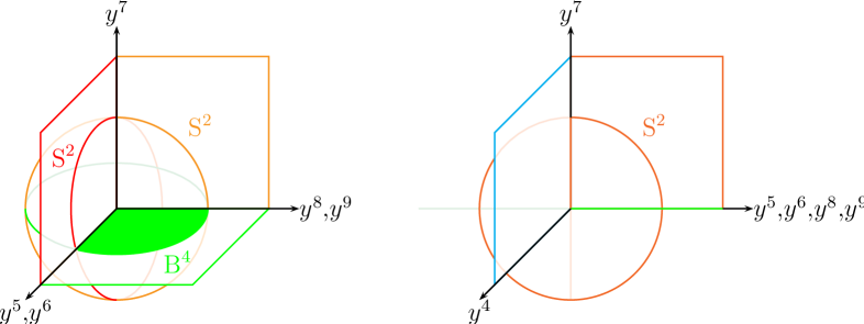
Figure 1: Directions of the polarization of the $\text{D}3$-branes in the $\mathcal{N}=2$ supersymmetric case $m_{1}=0$, $m_{2}=m_{3}=m$.

As shown in figure 1, the $\text{D}3$-branes are polarized into all their transverse directions except of $y^{4}$ with the same radius $r_{0}=\pi\alpha^{\prime}|c\zeta|m\sqrt{N^{2}-1}$, spanning a four-dimensional subspace. In the subplanes spanned by $y^{5}$, $y^{6}$, $y^{7}$ (depicted in red) and $y^{8}$, $y^{9}$, $y^{7}$ (depicted in orange), the coordinates are noncommutative, while in the subplane $y^{5}$, $y^{6}$, $y^{8}$, $y^{9}$ (depicted in green) the two sets of coordinates commute. The volume into which the $\text{D}3$-branes polarize is therefore a four-dimensional ball in the subplane $y^{5}$, $y^{6}$, $y^{8}$, $y^{9}$, where different values of $y^{7}$ correspond to different $\text{S}^{3}$ orbits within the ball. This configuration is symmetric under rotations of $y^{5}$, $y^{6}$, $y^{8}$, $y^{9}$ and hence should also lead to an embedding of a $\text{D}7$-brane which is symmetric under these rotations, e.g. which does only depend on the radial coordinate $\rho$. The $\text{D}3$-branes are also smeared out along these directions of the $\text{D}7$-branes. Since the $\text{D}3$-branes are only polarized into the direction $y^{7}$, this also means that the rotational invariance in the $y^{4}$, $y^{7}$ plane is lost. This corresponds to the breaking of the $U(1)$ symmetry.

For comparison let us also consider the ${\cal N}=1^{*}$ case where all adjoint chiral masses are equal. Here, the tensor components of $T_{3}$ in (B.19) become

$$T_{456}=iT_{789}=\frac{3m}{2\sqrt{2}}\leavevmode\nobreak\ ,\qquad iT_{459}=T_{678}=-iT_{468}=-T_{579}=iT_{567}=T_{489}=\frac{m}{2\sqrt{2}}\leavevmode\nobreak\ .$$ (2.27)

The $\text{D}3$-branes are also extended in the $y^{4}$-direction. There are $2$-spheres embedded in $y^{4}$, $y^{5}$, $y^{9}$. and in $y^{4}$, $y^{6}$, $y^{8}$, and as in the $\mathcal{N}=2$ case in $y^{5}$, $y^{6}$, $y^{7}$ and $y^{7}$, $y^{8}$, $y^{9}$, While the prior two have radius smaller by a factor $\frac{1}{2}$ w.r.t. $r_{0}$ in the $\mathcal{N}=2$ case discussed above, the latter two have a radius bigger by a factor of $\frac{3}{2}$. Hence, the projection as discussed before in the $\mathcal{N}=2$ case cannot longer be a simple $B^{4}$. The equations for the spheres including $y^{4}$ read

$$(y^{4})^{2}+(y^{5})^{2}+(y^{9})^{2}=\frac{r_{0}^{2}}{4}\leavevmode\nobreak\ ,\qquad(y^{4})^{2}+(y^{6})^{2}+(y^{8})^{2}=\frac{r_{0}^{2}}{4}\leavevmode\nobreak\ .$$ (2.28)

The polarization into the subspace $y^{4}$, $y^{5}$, $y^{6}$, $y^{8}$, $y^{9}$ then is similar to the one shown in the first picture in figure (1), but with a radius which is smaller by a factor of $\frac{1}{2}$, and an exchange e.g. of $y^{6}$ and $y^{9}$. The situation is different for the two $2$-spheres having in common $y^{7}$. Their equations read

$$(y^{5})^{2}+(y^{6})^{2}+(y^{7})^{2}=\frac{r_{0}^{2}}{4}\leavevmode\nobreak\ ,\qquad(y^{7})^{2}+(y^{8})^{2}+(y^{9})^{2}=\frac{9r_{0}^{2}}{4}\leavevmode\nobreak\ .$$ (2.29)

They are of different sizes. The above equations induce the relation

$$(y^{5})^{2}+(y^{6})^{2}+\frac{1}{9}(y^{8})^{2}+\frac{1}{9}(y^{9})^{2}=\frac{1}{2}r_{0}^{2}-\frac{10}{9}(y^{7})^{2}\leavevmode\nobreak\ .$$ (2.30)

At $y^{7}=\frac{1}{2}r_{0}$ one has $y^{5}=y^{6}=0$, and the equation becomes

$$(y^{8})^{2}+(y^{9})^{2}=2r_{0}^{2}\leavevmode\nobreak\ .$$ (2.31)

At $y^{7}=0$, one finds a rotational ellipsoid.

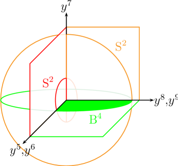
Figure 2: Directions of the polarization of the $\text{D}3$-branes in the equal mass case $m_{1}=m_{2}=m_{3}=m$.

Although topologically one still has a ball $\text{B}^{4}$, the difference in the length of the principal axes breaks the rotational symmetries in the $y^{5}$, $y^{6}$, $y^{8}$, $y^{9}$ plane. Still, the configuration is symmetric under rotations in the $y^{5}$, $y^{6}$ and $y^{8}$, $y^{9}$ planes, but it is no longer symmetric under rotating these planes into each other. This breaking of the underlying $SU(2)\times SU(2)$ symmetry into $U(1)\times U(1)$ prevents one from finding an embedding of a $\text{D}7$-brane depending on the radial coordinate $\rho$ in this plane only.

2.4 Symmetries and field theory action

We proceed by describing the $\text{D}7$-brane embedding and its symmetries. For comparison, we first recall the case of the undeformed $\text{AdS}_{5}\times\text{S}^{5}$ background [4, 5], in which the embedding of a $\text{D}7$-brane probe along $\text{AdS}_{5}\times\text{S}^{3}$ with zero distance from the background generating $\text{D}3$-branes breaks the original $SU(4)$ symmetry to $SU(2)\times SU(2)\times U(1)$, such that there is a remaining ${\cal N}=2$ supersymmetry. This scenario is displayed in figure 3.

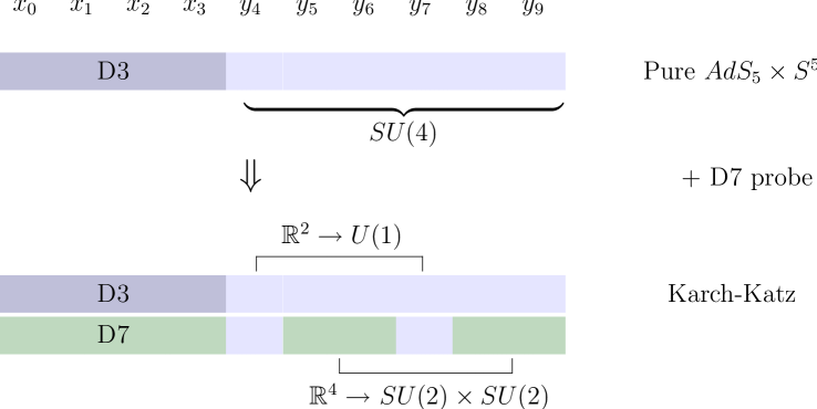
Figure 3: Symmetries for a $\text{D}7$-brane probe in $\text{AdS}_{5}\times\text{S}^{5}$.

Let us now consider the symmetries of the Polchinski-Strassler background with non-trivial $G_{3}$ flux at order $m^{2}$. For simplicity we consider the case in which $m_{1}=0$ and $m_{2}=m_{3}$ and, such that the background preserves ${\cal N}=2$ supersymmetry. As the discussion of section 2.3 shows (see equations (2.24) and (2.25) in particular), the background preserves a global $SU(2)\times SU(2)$ symmetry in this case. The background preserves two 2-spheres which have one direction in common. As (2.26) shows, $\rho$ is an invariant under this $SU(2)\times SU(2)\simeq SO(4)$. It is thus convenient to embed the $\text{D}7$-brane probe into the directions $y_{5}$, $y_{6}$, $y_{8}$, $y_{9}$. This embedding preserves the symmetries of the background. Note that the background does not have any further $U(1)$, which corresponds to the fact that superconformal symmetry is broken by the adjoint hyper mass terms. This embedding is displayed in figure 4. We denote the real directions $5,6,8,9$ along the $\text{D}7$-brane with indices $a,b$, and the directions $4,7$ perpendicular to it with $m,n$. In the complex coordinates (2.9), $a,b=2,3$ and $m=1$.

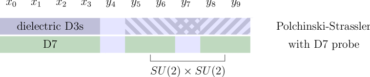
Figure 4: Symmetries for a $\text{D}7$-brane probe in the $\mathcal{N}=2$ Polchinski-Strassler background.

These symmetries are consistent with the symmetries of the ${\cal N}=2$ field theory in which the adjoint hypermultiplet is massive. The corresponding classical ${\cal N}=2$ Lagrangian is

$$\mathcal{L} =\operatorname{Im}\bigg{[}\tau\int\operatorname{d}\!^{2}\theta\operatorname{d}\!^{2}\bar{\theta}\big{(}\operatorname{tr}(\bar{\Phi}_{I}e^{V}\Phi_{I}e^{-V})+Q^{\dagger}e^{V}Q+\tilde{Q}e^{V}\tilde{Q}^{\dagger}\big{)}$$ (2.32)

$$\phantom{{}={}\operatorname{Im}\bigg{[}}+\tau\int\operatorname{d}\!^{2}\theta\big{(}\operatorname{tr}(\mathcal{W}^{\alpha}\mathcal{W}_{\alpha})+W\big{)}+\tau\int\operatorname{d}\!^{2}\bar{\theta}\big{(}\operatorname{tr}(\bar{\mathcal{W}}_{\dot{\alpha}}\bar{\mathcal{W}}^{\dot{\alpha}})+\bar{W}\big{)}\bigg{]}\leavevmode\nobreak\ ,$$

where the superpotential $W$ is

$$W=\operatorname{tr}\big{(}\epsilon^{pqr}\Phi_{p}\Phi_{q}\Phi_{r}+m(\Phi_{2}^{2}+\Phi_{3}^{2})\big{)}+\tilde{Q}(m_{\text{q}}+\Phi_{1})Q\leavevmode\nobreak\ .$$ (2.33)

The superfields $Q$ and $\tilde{Q}$ make up the $\mathcal{N}=2$ fundamental hypermultiplet. Following the assignment of charges of [5, 14], we observe that this Lagrangian has an $SU(2)\times SU(2)_{\text{R}}$ symmetry, where the first $SU(2)$ rotates the two complex scalars in each hypermultiplet into each other. The mass terms explicitly break the $U(1)$ symmetry of the $SU(2)\times U(1)$ superconformal group. This applies already to the adjoint mass term before turning on the fundamental fields, since the $U(1)$ charges of $\Phi_{2}$, $\Phi_{3}$ are zero, whereas a superconformal superpotential requires a $U(1)$ charge of $2$. Thus the field theory symmetries agree with the supergravity symmetries.

3 Forms

3.1 Summary

We have calculated the contributions to the background fields necessary for the $\text{D}7$-brane probe embedding at order $\mathcal{O}(m^{2})$. In particular the induced $C_{8}$ form, which has not been considered in the literature, is needed when adding $\text{D}7$-branes. Its computation is given below in section 3.2.

To summarize, the background RR and NSNS forms read

$$\begin{gathered}C_{4}=\operatorname{e}^{-\hat{\phi}}\Big{(}Z^{-1}+\frac{\zeta^{2}M^{2}R^{2}}{3^{4}2^{3}}Z^{-\frac{1}{2}}\Big{)}\operatorname{d}\!\operatorname{vol}(\mathds{R}^{1,3})+\frac{1}{2}B\wedge C_{2}\leavevmode\nobreak\ ,\qquad F_{5}=\operatorname{d}\!C_{4}+\star\operatorname{d}\!C_{4}\leavevmode\nobreak\ ,\end{gathered}$$ (3.2)

$$\begin{aligned} \tilde{C}_{2}&=\operatorname{e}^{-\hat{\phi}}\frac{\zeta}{3}Z\mbox{Re}\,S_{2}\leavevmode\nobreak\ ,\qquad&B&=-\frac{\zeta}{3}Z\mbox{Im}\,S_{2}\leavevmode\nobreak\ ,\qquad&G_{3}&=\operatorname{d}\!C_{2}-\tau\operatorname{d}\!B\leavevmode\nobreak\ ,\\ C_{6}&=\frac{2}{3}B\wedge\hat{C}_{4}\leavevmode\nobreak\ ,\qquad&B_{6}&=\frac{2}{3}C_{2}\wedge\hat{C}_{4}\leavevmode\nobreak\ ,\qquad&\star G_{3}&=\operatorname{d}\!C_{6}-\tau\operatorname{d}\!B_{6}\leavevmode\nobreak\ ,\\ \end{aligned}$$ (3.3)

$$\begin{gathered}C_{8}=-\frac{1}{6}\big{(}\operatorname{e}^{2\hat{\phi}}\tilde{C}_{2}\wedge\tilde{C}_{2}+B\wedge B\big{)}\wedge\hat{C}_{4}\leavevmode\nobreak\ ,\end{gathered}$$ (3.5)

where $\hat{C}_{4}$ denotes the unperturbed $4$-form potential given by the first term on the r.h.s. in the equation for $C_{4}$ above. The two types of corrections in $C_{4}$ are of order $\mathcal{O}(m^{2})$. One of them has components along the spacetime directions spanned by $x^{\mu}$, the other comes from the redefinition of the $4$-form (A.9) and has no components in these directions. It turns out that only $\hat{C}_{4}$ is relevant for a $\text{D}7$-brane embedding up to order $\mathcal{O}(m^{2})$. We also note that we can ignore the backreaction on $G_{3}$ itself, since it would be of order $\mathcal{O}(m^{3})$.

3.2 The $8$-form potential $C_{8}$

We show that the backreaction of $G_{3}$ on the background at order $m^{2}$ induces a non-vanishing $8$-form potential $C_{8}$ with field strength $\tilde{F}_{9}$. This potential couples to the $\text{D}7$-brane charge and hence has to be considered in an embedding of $\text{D}7$-branes in the Polchinski-Strassler background.

The physical field strengths are defined in (A.7). They are not all independent but are related to their corresponding Hodge duals according to (A.8). From these equations one finds, after transforming to Einstein frame with (A.12), that the $8$-form potential $C_{8}$ obeys the equation

$$\operatorname{d}\!C_{8}=\star\operatorname{d}\!C_{0}+\operatorname{d}\!B\wedge C_{6}\leavevmode\nobreak\ .$$ (3.6)

It therefore depends on the non-constant corrections to $C_{0}$ which start at order $m^{2}$ as well as on non-vanishing potentials $B$ and $C_{6}$. Taking the exterior derivative, thereby using that the $6$-form $C_{6}$ satisfies

$$\operatorname{d}\!C_{6}=-\star\tilde{F}_{3}+\operatorname{d}\!B\wedge C_{4}\leavevmode\nobreak\ ,$$ (3.7)

one finds

$$\operatorname{d}\!^{2}C_{8}=\operatorname{d}\!\star\operatorname{d}\!C_{0}+H_{3}\wedge\star\tilde{F}_{3}\leavevmode\nobreak\ .$$ (3.8)

This expression should vanish identically due to the nilpotency of the exterior derivative. Using the equation of motion for the axion found as the real part of (A.13) which up to quadratic order in the mass perturbation is given by

$$\operatorname{d}\!\star\operatorname{d}\!C_{0}=\frac{\operatorname{e}^{\hat{\phi}}}{2}\operatorname{Im}(G_{3}\wedge\star G_{3})=\operatorname{e}^{\hat{\phi}}\operatorname{Im}G_{3}\wedge\star\operatorname{Re}G_{3}=-H_{3}\wedge\star\tilde{F}_{3}\leavevmode\nobreak\ ,$$ (3.9)

this vanishing is evident. The reversed sign in the relation $\tilde{F}_{7}=-\star\tilde{F}_{3}$ of (A.8) is thereby crucial for the consistency.

Inserting the expression for $C_{6}$ (2.15) into (3.6) and then using (A.15) one finds that $C_{8}$ decomposes as

$$C_{8}=\omega_{4}\wedge\operatorname{d}\!\operatorname{vol}(\mathds{R}^{1,3})\leavevmode\nobreak\ ,$$ (3.10)

where $\omega_{4}$ is a $4$-form which has to be determined from the equation for the remaining components transverse to the worldvolume of the $\text{D}3$-branes

$$\operatorname{d}\!\omega_{4}=\star_{6}\operatorname{d}\!C_{0}-\operatorname{e}^{-\hat{\phi}}\frac{2\zeta}{9}\operatorname{d}\!B\wedge\operatorname{Im}S_{2}=\star_{6}\operatorname{d}\!C_{0}+\frac{2\zeta}{9}\operatorname{Im}G_{3}\wedge\operatorname{Im}S_{2}\leavevmode\nobreak\ .$$ (3.11)

The first term in (3.11) is found from the equation of motion for the complex dilaton-axion $\tau$ which reads after using (A.15) and neglecting terms beyond quadratic order in the masses

$$\operatorname{d}\!\star_{6}\operatorname{d}\!C_{0}=-\frac{\zeta}{18}(G_{3}\wedge\operatorname{d}\!S_{2}+\bar{G}_{3}\wedge\operatorname{d}\!\bar{S}_{2})\leavevmode\nobreak\ .$$ (3.12)

To find the r.h.s. we have also used the identity

$$\hat{Z}^{-1}(G_{3}\wedge\star_{6}G_{3}-\bar{G}_{3}\wedge\star_{6}\bar{G}_{3})=G_{3}\wedge\hat{Z}^{-1}(\star_{6}-i)G_{3}-\bar{G}_{3}\wedge\hat{Z}^{-1}(\star_{6}+i)\bar{G}_{3}$$ (3.13)

together with (2.14) and with (2.7). Considering the Bianchi identity $\operatorname{d}\!G_{3}=0$ this equation can be integrated easily and becomes

$$\star_{6}\operatorname{d}\!C_{0}=\frac{\zeta}{9}\operatorname{Re}(G_{3}\wedge S_{2})\leavevmode\nobreak\ .$$ (3.14)

Inserting this result, the equation (3.11) for $\omega_{4}$ then assumes the form

$$\operatorname{d}\!\omega_{4}=\frac{\zeta}{9}\operatorname{Re}(G_{3}\wedge\bar{S}_{2})=\operatorname{e}^{-\hat{\phi}}\frac{\zeta^{2}}{27}\operatorname{Re}(\operatorname{d}\!(\hat{Z}S_{2})\wedge\bar{S}_{2})\leavevmode\nobreak\ .$$ (3.15)

After some elementary manipulations the Bianchi identity $\operatorname{d}\!^{2}\omega_{4}=0$ becomes

$$\operatorname{d}\!(\operatorname{d}\!\hat{Z}\wedge S_{2}\wedge\bar{S}_{2})=0\leavevmode\nobreak\ .$$ (3.16)

Therefore $\operatorname{d}\!\hat{Z}\wedge S_{2}\wedge\bar{S}_{2}$ must follow from a $4$-form potential. The equation of motion (3.11) can be transformed to

$$\operatorname{d}\!\omega_{4} =\operatorname{e}^{-\hat{\phi}}\frac{\zeta^{2}}{54}\big{(}\operatorname{d}\!\hat{Z}\wedge S_{2}\wedge\bar{S}_{2}+\operatorname{d}\!(\hat{Z}S_{2}\wedge\bar{S}_{2})\big{)}\leavevmode\nobreak\ .$$ (3.17)

The Bianchi identity (3.16) thereby ensures that a potential for the first term and hence a $4$-form $\omega_{4}$ must exist. As shown in Appendix C, the first term in (3.17) can be rewritten as

$$\operatorname{d}\!\hat{Z}\wedge S_{2}\wedge\bar{S}_{2}=-2\operatorname{d}\!(\hat{Z}S_{2}\wedge\bar{S}_{2})\leavevmode\nobreak\ .$$ (3.18)

Using also the reexpression of $S_{2}$ in terms of $B$ and $\tilde{C}_{2}$ (2.13), the $4$-form potential therefore reads

$$\omega_{4} =-\operatorname{e}^{-\hat{\phi}}\frac{\zeta^{2}}{54}\hat{Z}S_{2}\wedge\bar{S}_{2}=-\frac{\operatorname{e}^{-\hat{\phi}}}{6}\hat{Z}^{-1}(\operatorname{e}^{2\hat{\phi}}\tilde{C}_{2}\wedge\tilde{C}_{2}+B\wedge B)\leavevmode\nobreak\ ,$$ (3.19)

and together with (3.10) it determines $C_{8}$. Using the expression for $\hat{C}_{4}$ (2.4), one then finds

$$C_{8}=-\frac{1}{6}(\operatorname{e}^{2\hat{\phi}}\tilde{C}_{2}\wedge\tilde{C}_{2}+B\wedge B)\wedge\hat{C}_{4}\leavevmode\nobreak\ .$$ (3.20)

4 $\text{D}7$-brane action

With these ingredients we are now able to calculate the action for the probe $\text{D}7$-brane in this background, which we present below. Moreover we derive the equation of motion from this action and discuss possible solutions for the brane embedding.

4.1 The action

The action for a $\text{D}7$-brane in the Einstein frame is given by

$$S =S_{\mathrm{DBI}}+S_{\mathrm{CS}}\leavevmode\nobreak\ ,$$ (4.1)

$$S_{\mathrm{DBI}} =-T_{7}\operatorname{e}^{-2\hat{\phi}}\int\operatorname{d}\!^{8}\xi\operatorname{e}^{\phi}\sqrt{\big{|}\det P\big{[}g-\operatorname{e}^{-\frac{\phi-\hat{\phi}}{2}}B\big{]}+2\pi\alpha^{\prime}\operatorname{e}^{-\frac{\phi-\hat{\phi}}{2}}F\big{|}}\leavevmode\nobreak\ ,$$ (4.2)

$$S_{\mathrm{CS}} =-\mu_{7}\int\sum\limits_{r=1}^{4}P\big{[}C_{2r}\wedge\operatorname{e}^{-B}\big{]}\wedge\operatorname{e}^{2\pi\alpha^{\prime}F}\leavevmode\nobreak\ ,$$ (4.3)

where $T_{7}=\mu_{7}$. We use the conventions of [21], in which the transformation between the Einstein and string frame metric contains just the non-constant part $\phi-\hat{\phi}$ of the dilaton $\phi$, where $\operatorname{e}^{\hat{\phi}}=g_{\text{s}}$ is the string coupling constant. See appendix A for details.

In static gauge, the pullback of a generic $2$-tensor $E$ is defined by

$$P[E]_{ab} =E_{ab}+\partial_{a}X^{m}E_{mb}+\partial_{b}X^{n}E_{an}+\partial_{a}X^{m}\partial_{b}X^{n}E_{mn}\leavevmode\nobreak\ .$$ (4.4)

Note the minus sign in (4.3). In principle for the $AdS_{5}\times S^{5}$ background, there is a convention choice here corresponding to the sign choice in the projector $\varepsilon=\pm\Gamma\varepsilon$ for the supersymmetries preserved by the brane. However in the ${\cal N}=2$ Polchinski-Strassler background, there remains only one choice consistent with the supersymmetries of the background. The correct choice corresponds to the minus sign in (4.3). This is also in agreement with [3, 38, 30].

Using the explicit expression for the induced forms $C_{6}$ and $C_{8}$ as in (2.15) (3.20), the Chern-Simons part at order $\mathcal{O}(m^{2})$ reduces to ($P[F]=F$)

$$S_{\mathrm{CS}} =-\mu_{7}\int P\Big{[}\hat{C}_{4}\wedge\Big{(}-\frac{1}{3}B\wedge(B+2\pi\alpha^{\prime}F)+2\pi^{2}\alpha^{\prime 2}F\wedge F-\frac{1}{6}\operatorname{e}^{2\hat{\phi}}\tilde{C}_{2}\wedge\tilde{C}_{2}\Big{)}\Big{]}\leavevmode\nobreak\ .$$ (4.5)

We now expand to quadratic order in the mass perturbation around the unperturbed metric (2.1). For the total $\text{D}7$-brane action we find in appendix D

$$S =-T_{7}\operatorname{e}^{-\hat{\phi}}\int\operatorname{d}\!^{8}\xi\sqrt{\det P[\delta]_{ab}}\Big{[}1+\tilde{\phi}+\frac{1}{2}Z^{\frac{1}{2}}\tilde{g}_{\mu\mu}+\frac{1}{2}Z^{-\frac{1}{2}}P[\delta]^{ab}P[\tilde{g}]_{ab}$$ (4.6)

$$\phantom{={}-T_{7}\operatorname{e}^{-\hat{\phi}}\int\operatorname{d}\!^{8}\xi\sqrt{\det P[\delta]_{ab}}\Big{[}}+\frac{1}{2}Z^{-1}\Big{(}\Big{(}1-\frac{2}{3}\star_{4}\Big{)}P[B]\cdot P[B]$$

$$\phantom{={}-T_{7}\operatorname{e}^{-\hat{\phi}}\int\operatorname{d}\!^{8}\xi\sqrt{\det P[\delta]_{ab}}\Big{[}+\frac{1}{2}Z^{-1}\Big{(}}-4\pi\alpha^{\prime}\Big{(}1+\frac{1}{3}\star_{4}\Big{)}F\cdot P[B]$$

$$\phantom{={}-T_{7}\operatorname{e}^{-\hat{\phi}}\int\operatorname{d}\!^{8}\xi\sqrt{\det P[\delta]_{ab}}\Big{[}+\frac{1}{2}Z^{-1}\Big{(}}+4\pi^{2}\alpha^{\prime 2}(1+\star_{4})F\cdot F \phantom{={}-T_{7}\operatorname{e}^{-\hat{\phi}}\int\operatorname{d}\!^{8}\xi\sqrt{\det P[\delta]_{ab}}\Big{[}+\frac{1}{2}Z^{-1}\Big{(}}-P[B]\cdot\star_{4}P[B]-\frac{4}{3}P[B]\cdot\star_{4}F$$

$$\phantom{={}-T_{7}\operatorname{e}^{-\hat{\phi}}\int\operatorname{d}\!^{8}\xi\sqrt{\det P[\delta]_{ab}}\Big{[}+\frac{1}{2}Z^{-1}\Big{(}}-\frac{1}{3}\operatorname{e}^{2\hat{\phi}}P[\tilde{C}_{2}]\cdot\star_{4}P[\tilde{C}_{2}]\Big{)}\Big{)}\Big{]}\leavevmode\nobreak\ ,$$

where throughout the paper with a ‘tilde’ we denote the order $\mathcal{O}(m^{2})$ corrections to the unperturbed quantities which carry a ‘hat’. We should stress that here the four-dimensional inner product $\cdot$ as well as the Hodge star $\star_{4}$ are understood to be computed with the pullback metric according to (A.16) and (A.17), respectively.

We are going to discuss the equation of motion derived from this action in detail below. However first let us mention why we can neglect the backreaction of the $\text{D}7$-brane on the background. First, as in all probe approximations within AdS/CFT, we have a large number $N$ of background generating $\text{D}3$-branes compared to only a single $\text{D}7$-brane. In the limit $N\to\infty$, $g_{\text{s}}N=\text{fixed}$, the backreaction on the unperturbed $\text{AdS}_{5}\times\text{S}^{5}$ part is negligible. It is of order $g_{\text{s}}N_{\text{f}}$, where $N_{\text{f}}$ is a fixed number of $\text{D}7$-branes [4]. However for the Polchinski-Strassler background, we also have to be sure that the backreaction on the perturbation parameterized by $G_{3}$ is negligible. Otherwise, we would have to consider its effect in the equations of motion from the type II B supergravity action $S_{\text{II}\,\text{B}}$ before determining $G_{3}$ and the correction of the background. In other words, the backreaction of the $\text{D}7$-brane must not be of the same order as the perturbation of the background by $G_{3}$. We see that this is indeed the case: Since $S_{\text{II}\,\text{B}}\sim\operatorname{e}^{-2\hat{\phi}}$ whereas $S\sim\operatorname{e}^{-\hat{\phi}}$, the $\text{D}7$-brane contributes to the background equations of motion at relative order $g_{\text{s}}$.

4.2 Gauge field sources

The action (4.6) contains a linear coupling of the gauge field $F$ to the NSNS field $B$, generating a source term in the equation of motion for $F$. Since the corresponding $F$ is proportional to $\frac{1}{2\pi\alpha^{\prime}}$, it cannot be neglected in the analysis. The equation of motion for $F$ reads

$$\operatorname{d}\!\Big{(}\hat{C}_{4}\wedge\Big{(}2\pi\alpha^{\prime}(\star_{4}+1)F-\Big{(}\star_{4}+\frac{1}{3}\Big{)}P[B]\Big{)}\Big{)}=0\leavevmode\nobreak\ .$$ (4.7)

Integrating the above equation, and decomposing it with (B.16) into its components purely along (anti-)holomorphic directions and along mixed directions, one finds

$$2Z^{-1}\Big{(}2\pi\alpha^{\prime}F_{(1,1)}^{\text{P}}-\frac{2}{3}P[B]_{(1,1)}\Big{)}=\omega_{(1,1)}\leavevmode\nobreak\ ,\qquad-\frac{2}{3}Z^{-1}P[B]_{(2,0)}=\omega_{(2,0)}\leavevmode\nobreak\ ,$$ (4.8)

where we have omitted to indicate with an index P also the primitive part of $P[B]_{(1,1)}$ since it is primitive anyway. The $2$-form $\omega_{2}$ is closed. A separation of this condition into its individual components leads to the equations

$$\partial\omega_{(2,0)}=0\leavevmode\nobreak\ ,\qquad\bar{\partial}\omega_{(2,0)}+\partial\omega_{(1,1)}=0\leavevmode\nobreak\ ,$$ (4.9)

where $\partial$ and $\bar{\partial}$ is the holomorphic and the antiholomorphic part of the exterior derivative operator $\operatorname{d}\!{}$. The first equation is trivially satisfied, since the subspace on which the above forms are defined is only four-dimensional. From the second equation one derives

$$\partial\Big{(}Z^{-1}\Big{(}2\pi\alpha^{\prime}F_{(1,1)}^{\text{P}}-\frac{2}{3}P[B]_{(1,1)}\Big{)}\Big{)}=\frac{1}{3}\bar{\partial}\big{(}Z^{-1}P[B]_{(2,0)}\big{)}\leavevmode\nobreak\ .$$ (4.10)

The above equation is part of the full equation of motion, which reads

$$\partial\Big{(}4\pi\alpha^{\prime}Z^{-1}F_{(1,1)}^{\text{P}}+\frac{\zeta}{9}\Big{(}4P[\operatorname{Im}S_{2}]_{(1,1)}-i\bar{\partial}\varphi\Big{)}\Big{)}$$ (4.11)

$$+\bar{\partial}\Big{(}4\pi\alpha^{\prime}Z^{-1}F_{(1,1)}^{\text{P}}+\frac{\zeta}{9}\Big{(}4P[\operatorname{Im}S_{2}]_{(1,1)}+i\partial\bar{\varphi}\Big{)}\Big{)}$$

$$-\frac{\zeta}{9}(\partial+\bar{\partial})\Big{(}2P[\operatorname{Im}S_{2}]_{(2,0)}+2P[\operatorname{Im}S_{2}]_{(0,2)}+i(\partial\varphi-\bar{\partial}\bar{\varphi})\Big{)}=0\leavevmode\nobreak\ .$$

We have extended the above equation by introducing a $1$-form $\varphi$ with only holomorphic components, which in total does not give any contribution. The reason for this procedure will become clear below.

Without a priori knowledge of the embedding it seems to be impossible to integrate the above equation without further input or assumptions. The reason for this is the non-vanishing of the last term in the above equation. It is present because the coefficients in the linear combination with $\star_{4}$ acting on $P[B]$ in the equation or motion (4.7) do not coincide with the ones in front of $F$. This term would be absent if also a projector $1+\star_{4}$ acted on $P[B]$. One can easily integrate the equation of motion under the assumption that the last term above is vanishing, e.g.

$$(\partial+\bar{\partial})\Big{(}P[\operatorname{Im}S_{2}]_{(2,0)}+P[\operatorname{Im}S_{2}]_{(2,0)}+\frac{i}{2}(\partial\varphi-\bar{\partial}\bar{\varphi})\Big{)}=0\leavevmode\nobreak\ .$$ (4.12)

In this case a solution for $F$ is immediately found as

$$4\pi\alpha^{\prime}Z^{-1}F=-\frac{\zeta}{9}(2(1+\star_{4})P[\operatorname{Im}S_{2}]-i(\bar{\partial}\varphi-\partial\bar{\varphi}))+\operatorname{d}\!A_{0}\leavevmode\nobreak\ ,$$ (4.13)

where we have introduced an exact form $\operatorname{d}\!A_{0}$ which is a solution of the vacuum equations of motion for $F$.

In Appendix B we show that the pullback of the imaginary part of $S_{2}$ decomposes as

$$P[\operatorname{Im}S_{2}]_{(2,0)} =3\operatorname{Im}S_{(2,0)}^{\parallel}-\frac{i}{2}\partial\theta\leavevmode\nobreak\ ,$$ (4.14)

$$P[\operatorname{Im}S_{2}]_{(1,1)} =3\operatorname{Im}S_{(1,1)}^{\parallel}-\frac{i}{2}(\bar{\partial}\theta-\partial\bar{\theta})\leavevmode\nobreak\ ,$$

$$P[\operatorname{Im}S_{2}]_{(0,2)} =3\operatorname{Im}S_{(0,2)}^{\parallel}+\frac{i}{2}\bar{\partial}\bar{\theta}\leavevmode\nobreak\ ,$$

where with $\parallel$ we indicate the components along the directions of the $\text{D}7$-brane explicitly given in (B.23). Furthermore, $\theta$ is a $1$-form defined by

$$\theta=\theta_{(1,0)} =(\bar{T}_{m\bar{a}b}\bar{z}^{a}z^{m}+\bar{T}_{\bar{m}ab}z^{a}\bar{z}^{m}-T_{\bar{m}\bar{a}b}\bar{z}^{a}\bar{z}^{m})\operatorname{d}\!z^{b}\leavevmode\nobreak\ .$$ (4.15)

The components of the condition (4.12) can be separated, and one uses the first of the above relations (4.14) to obtain

$$\bar{\partial}\Big{(}P[\operatorname{Im}S_{2}]_{(2,0)}+\frac{i}{2}\partial\varphi\Big{)} =\bar{\partial}\Big{(}3\operatorname{Im}S_{(2,0)}^{\parallel}-\frac{i}{2}\partial(\theta-\varphi)\Big{)}=0\leavevmode\nobreak\ .$$ (4.16)

The first term in the above equation explicitly reads with the definition of $S_{2}$ in (2.8) in the complex basis

$$\operatorname{Im}S_{(2,0)}^{\parallel}=\frac{i}{4}\bar{T}_{\bar{m}ab}\operatorname{d}\!z^{a}\wedge\operatorname{d}\!z^{b}=0\leavevmode\nobreak\ .$$ (4.17)

It vanishes since it is proportional to $m_{1}=0$. The condition (4.16) is then easily satisfied for an appropriately chosen $\varphi$, e.g. given by

$$\varphi=\theta+\partial h\leavevmode\nobreak\ .$$ (4.18)

We have introduced a function $h$ whose holomorphic derivative is part of the homogeneous solution. Inserting the result for $\varphi$, the solution for $F$ (4.13) hence becomes

$$4\pi\alpha^{\prime}Z^{-1}F=-\frac{\zeta}{9}(2(1+\star_{4})P[\operatorname{Im}S_{2}]-i(\partial\bar{\theta}-\bar{\partial}\theta))+\operatorname{d}\!A_{0}\leavevmode\nobreak\ .$$ (4.19)

One then uses the second relation in (4.14) to eliminate the $\theta$-dependent terms. The result for $F$ then reads

$$4\pi\alpha^{\prime}Z^{-1}F =-\frac{\zeta}{3}(1+\star_{4})(P[\operatorname{Im}S_{2}]-\operatorname{Im}S_{2}^{\parallel}))+\operatorname{d}\!A_{0}\leavevmode\nobreak\ .$$ (4.20)

Using the relation (2.13) to reexpress the imaginary parts of $S_{2}$ in terms of $B$, one finally finds

$$2\pi\alpha^{\prime}F =\frac{1}{2}(1+\star_{4})(P[B]-B^{\parallel})+\frac{Z}{2}\operatorname{d}\!A_{0}\leavevmode\nobreak\ .$$ (4.21)

It is worth to remark that by using the expression for the pullback in static gauge, the linear combination keeps only the derivative terms of the embedding coordinates that come from the pullback. This is a particularity for the coefficients in the linear combination with $\star_{4}$ in front of $P[B]$ in the equation of motion (4.7).

4.3 Expansion of the embedding

At sufficient distance from the polarized brane source, the Polchinski-Strassler background is given by $\text{AdS}_{5}\times\text{S}^{5}$ with corrections at quadratic order in the mass perturbation. One can therefore expand the full embedding coordinates $X^{m}\equiv y^{m}$, $m=4,7$ into a known unperturbed part $\hat{X}^{m}$, which is the constant embedding in $\text{AdS}_{5}\times\text{S}^{5}$ and into a perturbation $\tilde{X}^{m}$, i.e.

$$X^{m}=\hat{X}^{m}+\tilde{X}^{m}\leavevmode\nobreak\ .$$ (4.22)

This decomposition is inserted into the complete action. Then one expands in powers of $\tilde{X}^{m}$, thereby including all corrections to the background such that the resulting equations of motion contain all terms up to quadratic order in the mass perturbation. This yields differential equations for $\tilde{X}^{m}$. In the case of the $\mathcal{N}=2$ embedding to be discussed below, it becomes an ordinary differential equation of second order that can be solved analytically. However, the solution found in this way is accurate only in a regime where the bare embedding coordinates dominate the correction, i.e. where $\hat{X}^{m}\gtrsim\tilde{X}^{m}$.

Inserting (4.22) and the corresponding decompositions for all background fields, as well as the expressions (2.15) and (3.20) for the induced $C_{6}$ and $C_{8}$, one finds that for a constant unperturbed embedding the action (4.6) becomes up to quadratic order in the perturbation

$$S =-T_{7}\operatorname{e}^{-\hat{\phi}}\int\operatorname{d}\!^{8}\xi\Big{[}1+\tilde{\phi}+\frac{1}{2}Z^{\frac{1}{2}}\tilde{g}_{\mu\mu}+\frac{1}{2}Z^{-\frac{1}{2}}\tilde{g}_{aa}+\frac{1}{2}(\partial_{a}\tilde{X}^{m})^{2}+Z^{-\frac{1}{2}}\partial_{a}\tilde{X}^{m}\tilde{g}_{ma}$$ (4.23)

$$\phantom{=-T_{7}\operatorname{e}^{-\hat{\phi}}\int\operatorname{d}\!^{8}\xi\Big{[}}+\frac{1}{2}Z^{-1}\Big{(}\Big{(}1-\frac{2}{3}\star_{4}\Big{)}B\cdot(B+4\partial\tilde{X}B)$$

$$\phantom{=-T_{7}\operatorname{e}^{-\hat{\phi}}\int\operatorname{d}\!^{8}\xi\Big{[}+\frac{1}{4}Z^{-1}\Big{(}}-4\pi\alpha^{\prime}\Big{(}1+\frac{1}{3}\star_{4}\Big{)}F\cdot\big{(}B+2\partial\tilde{X}B\big{)}+4\pi^{2}\alpha^{\prime 2}(1+\star_{4})F\cdot F$$

$$\phantom{=-T_{7}\operatorname{e}^{-\hat{\phi}}\int\operatorname{d}\!^{8}\xi\Big{(}+\frac{1}{4}Z^{-1}\Big{(}}-\frac{1}{3}\operatorname{e}^{2\hat{\phi}}\star_{4}\tilde{C}\cdot\big{(}\tilde{C}+4\partial\tilde{X}\tilde{C}\big{)}\Big{)}\Big{]}\leavevmode\nobreak\ .$$

Since the action at this order does not include terms that depend on the mass perturbation and include the perturbation $\tilde{X}^{m}$ at quadratic order, the Hodge star and the inner product as defined in (A.1), (A.5) become the ordinary ones in flat space for the constant unperturbed embedding. It is also important to remark that in the above expansion terms that are quadratic in the mass perturbation but in addition linear in the perturbation of the embedding $\tilde{X}^{m}$ have been kept. This ensures that in the equations of motion for the fluctuations all terms that are quadratic in the perturbation do appear.

In the above equation we have used the abbreviations

$$(\partial\tilde{X}B)_{ab}=\partial_{a}\tilde{X}^{m}B_{mb}\leavevmode\nobreak\ ,\qquad(B\partial\tilde{X})_{ab}=\partial_{b}\tilde{X}^{m}B_{am}\leavevmode\nobreak\ .$$ (4.24)

They are also of use for an expansion of the expression (4.21) for the gauge field strength $F$, which becomes

$$2\pi\alpha^{\prime}F=\frac{1}{2}(1+\star_{4})(\partial\tilde{X}B+B\partial\tilde{X})\leavevmode\nobreak\ ,$$ (4.25)

and in which we have neglected $A_{0}$ that does not contribute to the source terms. The previously mentioned dependence of $F$ only on derivative terms of the embedding is now obvious. Since $F$ is thus of linear order in the mass perturbation and in the corrections to the embedding, one can directly neglect all terms quadratic in $F$ as well as all terms that contain $F$ and additional dependence of linear order in $\tilde{X}$. The action thus becomes

$$S =-T_{7}\operatorname{e}^{-\hat{\phi}}\int\operatorname{d}\!^{8}\xi\Big{[}1+\tilde{\phi}+\frac{1}{2}Z^{\frac{1}{2}}\tilde{g}_{\mu\mu}+\frac{1}{2}Z^{-\frac{1}{2}}\tilde{g}_{aa}+\frac{1}{2}(\partial_{a}\tilde{X}^{m})^{2}+Z^{-\frac{1}{2}}\partial_{a}\tilde{X}^{m}\tilde{g}_{ma}$$ (4.26)

$$\phantom{=-T_{7}\operatorname{e}^{-\hat{\phi}}\int\operatorname{d}\!^{8}\xi\Big{[}}+\frac{1}{2}Z^{-1}\Big{(}\Big{(}1-\frac{2}{3}\star_{4}\Big{)}B\cdot B+\frac{4}{3}(1-4\star_{4})B\cdot\partial\tilde{X}B$$

$$\phantom{=-T_{7}\operatorname{e}^{-\hat{\phi}}\int\operatorname{d}\!^{8}\xi\Big{(}+\frac{1}{4}Z^{-1}\Big{(}}-\frac{1}{3}\operatorname{e}^{2\hat{\phi}}\star_{4}\tilde{C}\cdot\big{(}\tilde{C}+4\partial\tilde{X}\tilde{C}\big{)}\Big{)}\Big{]}\leavevmode\nobreak\ ,$$

where we have also made use of the fact that $\star_{4}^{2}=1$.

To present the equations of motion, it is advantageous to transform to polar coordinates. The two directions transverse to the $\text{D}7$-brane become

$$X^{4} =u\cos\psi=\hat{u}\cos\hat{\psi}-\hat{u}\tilde{\psi}\sin\hat{\psi}+\tilde{u}\cos\hat{\psi}\leavevmode\nobreak\ ,$$ (4.27)

$$X^{7} =u\sin\psi=\hat{u}\sin\hat{\psi}+\hat{u}\tilde{\psi}\cos\hat{\psi}+\tilde{u}\sin\hat{\psi}\leavevmode\nobreak\ ,$$

where in the final expressions we have expanded up to linear order in the perturbations $\tilde{u}$ and $\tilde{\psi}$ of the radius and angular dependence, respectively.

As shown in appendix E, the equations of motions assume the form

$$\frac{1}{\rho^{3}}\partial_{\rho}(\rho^{3}\partial_{\rho}f(\rho))=g(\rho)\leavevmode\nobreak\ ,\qquad g(\rho)=\frac{\hat{u}}{\hat{r}^{4}}\Big{(}B_{f}+\frac{\hat{u}^{2}}{\hat{r}^{2}}C_{f}\Big{)}\leavevmode\nobreak\ ,\qquad\hat{r}^{2}=\hat{r}^{2}(\rho)=\rho^{2}+\hat{u}^{2}\leavevmode\nobreak\ ,$$ (4.28)

where $f=u$ or $f=\psi$ and $B_{f}$ and $C_{f}$ are constants that depend on the unperturbed embedding coordinates $\hat{u}$, $\hat{\psi}$ and which are of quadratic order in the mass perturbation. We should remark that without the inhomogenity, i.e. $B_{f}=C_{f}=0$, the above equation is the one found for the embedding of $\text{D}7$-branes in pure $\text{AdS}_{5}\times\text{S}^{5}$ at large $r$. Furthermore, the constant embedding $\hat{u}=0$ therefore remains a solution also in presence of the mass perturbation. Note that $\hat{u}$ is identified with the quark mass by virtue of $\hat{u}=2\pi\alpha^{\prime}m_{\text{q}}$.

We discuss the case $\hat{u}\neq 0$. For $f=u$ the constants $B$ and $C$ read

$$B_{u}=\frac{\zeta^{2}m^{2}R^{4}}{54}(-4+\cos 2\hat{\psi})\leavevmode\nobreak\ ,\qquad C_{u}=\frac{\zeta^{2}m^{2}R^{4}}{81}(-10+3\cos 2\hat{\psi})\leavevmode\nobreak\ .$$ (4.29)

For $f=\psi$ one has to identify

$$B_{\psi}=-\frac{\zeta^{2}m^{2}R^{4}}{54\hat{u}}\sin 2\hat{\psi}\leavevmode\nobreak\ ,\qquad C_{\psi}=-\frac{2\zeta^{2}m^{2}R^{4}}{27\hat{u}}\sin 2\hat{\psi}\leavevmode\nobreak\ .$$ (4.30)

The full solution of the differential equation (4.28) reads

$$f(\rho)=\hat{f}+\frac{A_{f}}{\rho^{2}}-\frac{B_{f}}{4}\frac{\hat{u}}{\rho^{2}}(1+\ln\hat{r}^{2})+\frac{C_{f}}{8}\frac{\hat{u}^{3}}{\rho^{2}\hat{r}^{2}}=\hat{f}+\frac{1}{8\rho^{2}}\Big{(}C_{f}\frac{\hat{u}^{3}}{r^{2}}+2(4A_{f}-B_{f}\hat{u})-2B_{f}\hat{u}\ln\hat{r}^{2}\Big{)}\leavevmode\nobreak\ ,$$ (4.31)

where $\hat{f}$ is the unperturbed value of $f$ which is the value of $f$ at the boundary at $\rho\to\infty$. $A_{f}$ is an integration constant that has to be fixed by the condition that the solution does not become singular at $\rho=0$. In the unperturbed $\text{AdS}_{5}\times\text{S}^{5}$ case one would have to set $A_{f}=0$. Here, in contrast, we have to allow $A_{f}\neq 0$ to find a non-singular embedding.

For an embedding that becomes singular at $\rho=0$ the decomposition in (4.22) used to expand the action and equations of motion is only justified for $\rho\gtrsim mR^{2}$, for which $\hat{X}^{m}\gtrsim\tilde{X}^{m}$ holds. This means a more restrictive constraint than the condition under which the Polchinski-Strassler background is given by an expansion around the $\text{AdS}_{5}\times\text{S}^{5}$ background, requiring only that $r\gtrsim mR^{2}$. For the embedding regular at $\rho=0$, however, there is no restriction on $\rho$. We only have to take care that it does not enter the regime where the perturbative description of the background breaks down. We will see that the $\text{D}7$-branes avoid to enter the region of small $r$. For the expansion (4.22) we only have to keep in mind that it is a good approximation only when $\hat{X}^{m}\gtrsim mR^{2}$ such that the corrections $\tilde{X}^{m}$ are small.

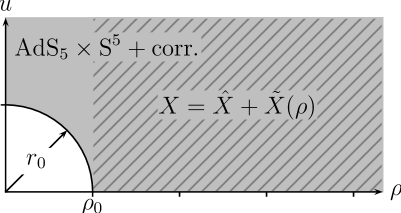
Figure 5: The two radial directions $\rho$ and $u$ in the six-dimensional space perpendicular to $x^{\mu}$. In the grayscaled region, the perturbative treatment of the backreaction around $\text{AdS}_{5}\times\text{S}^{5}$ is valid. In the hatched region, the expansion of the embedding $X^{m}$ into the constant embedding $\hat{X}$ plus a small $\rho$-dependent correction is valid. For regular embeddings the decomposition is valid also for $\rho<\rho_{0}$, provided $r\geq mR^{2}$. At radii smaller than $r_{0}\sim mR^{2}$, the backreaction becomes strong, and the background cannot be described by $\text{AdS}_{5}\times\text{S}^{5}$ plus corrections.

In the following we determine $A_{f}$ to cancel the divergence at $\rho\to 0$ which leads to the regular solution. We find in the limit $\rho^{2}\ll u^{2}$

$$f(\rho)\sim\hat{f}-\frac{C_{f}}{8\hat{u}}-\frac{B_{f}}{4\hat{u}}+\frac{1}{8\rho^{2}}\Big{(}8A_{f}-2B_{f}\hat{u}(1+\ln\hat{u}^{2})+C_{f}\hat{u}\Big{)}\leavevmode\nobreak\ .$$ (4.32)

From this expansion it follows that there exist non-singular solutions in the special case

$$8A_{f}-2B_{f}\hat{u}(1+\ln\hat{u}^{2})+C_{f}\hat{u}=0\leavevmode\nobreak\ .$$ (4.33)

In this case the full solution, which is regular on $0\leq\rho<\infty$, reads

$$f(\rho)=\hat{f}-C_{f}\frac{\hat{u}}{8\hat{r}^{2}}-B_{f}\frac{\hat{u}}{4\rho^{2}}\ln\frac{\hat{r}^{2}}{\hat{u}^{2}}\leavevmode\nobreak\ .$$ (4.34)

It has the asymptotic behaviour

$$\rho\to 0: \qquad f(\rho)\sim\hat{f}-\frac{1}{8\hat{u}}(2B_{f}+C_{f})\leavevmode\nobreak\ ,$$ (4.35)

$$\rho\to\infty: \qquad f(\rho)\sim\hat{f}-B_{f}\frac{\hat{u}}{4\rho^{2}}\ln\rho^{2}-\frac{\hat{u}}{8\rho^{2}}\Big{(}C_{f}-2B_{f}\ln\hat{u}^{2}\Big{)}\leavevmode\nobreak\ .$$

Considering the values $B_{\psi}$ and $C_{\psi}$ which determine the angular dependence of the solution, no $\rho$ dependent perturbation is found for the unperturbed embedding with $\hat{\psi}=0$, where $u=X^{4}$, or $\hat{\psi}=\frac{\pi}{2}$, where $u=X^{7}$. According to figure 1, $y^{7}$ is the only direction into which the $\text{D}3$-branes polarize and which is not parallel to the directions of the $\text{D}7$-brane. The two choices $\hat{\psi}=0$ and $\hat{\psi}=\frac{\pi}{2}$ are singled out, since the polarization direction is respectively perpendicular or along the direction of the separation of the two types of branes.

4.4 Holographic renormalization

The embedding solutions we have derived in the previous section are not constant. We may therefore wonder if their boundary behaviour for $\rho\rightarrow\infty$ might imply the presence of a VEV for the fermion bilinear which would violate supersymmetry. In this section we show that such a fermion condensate is absent. For this, suitable finite counterterms have to be added to the action, such that it vanishes when evaluated on a solution, as required by supersymmetry. According to [42, 43], this addition of counterterms corresponds to a change of renormalization scheme. If we were able to find the canonical coordinates for our background, i.e. those in which the kinetic term is canonically normalized in presence of the order $\mathcal{O}(m^{2})$ corrections, an addition of finite counterterms would not be necessary.

The holographic renormalization of the expanded $\text{D}7$-brane action (4.23) or correspondingly (4.26) is best performed in the coordinate system introduced in [42]. These are essentially Poincaré coordinates in which the $\text{AdS}_{5}$ metric (2.1) is given by

$$\operatorname{d}\!s^{2}=\frac{1}{R^{2}\chi}\eta_{\mu\nu}\operatorname{d}\!x^{\mu}\operatorname{d}\!x^{\nu}+\frac{R^{2}}{4\chi}\operatorname{d}\!\chi\leavevmode\nobreak\ .$$ (4.36)

The only replacement to be done is a redefinition of the holographic direction. Instead of $\rho$ one chooses

$$r=\frac{1}{\sqrt{\chi}}\leavevmode\nobreak\ ,\qquad\frac{\rho\operatorname{d}\!\rho}{r}=-\frac{\operatorname{d}\!\chi}{2\sqrt{\chi}^{3}}\leavevmode\nobreak\ ,\qquad\rho\operatorname{d}\!\rho=-\frac{\operatorname{d}\!\chi}{2\chi^{2}}\leavevmode\nobreak\ ,\qquad\partial_{\rho}=-2\rho\chi^{2}\partial_{\chi}\leavevmode\nobreak\ .$$ (4.37)

In the special case $m_{1}=0$, $m_{2}=m_{3}=m$ the action in the new coordinates is derived in Appendix F. Keeping all terms up to order $\mathcal{O}(m^{2})$ in the on-shell action (F.11), the regularized action is found to be given by

$$S_{\text{reg}} =-\frac{T_{7}}{2}\operatorname{e}^{-\hat{\phi}}\Omega_{3}\int\operatorname{d}\!\xi^{4}\,\Big{[}-\frac{1}{2\hat{\chi}^{2}}+\frac{\hat{u}^{2}}{\hat{\chi}}+\frac{\zeta^{2}m^{2}R^{4}}{108}\Big{(}-\frac{5}{3\hat{\chi}}+\Big{(}c_{0}-\frac{5}{3}\Big{)}\hat{u}^{2}\ln\hat{\chi}-c_{0}\hat{u}^{4}\hat{\chi}\Big{)}\Big{]}_{\epsilon}^{\frac{1}{\hat{u}^{2}}}$$ (4.38)

$$=-\frac{T_{7}}{2}\operatorname{e}^{-\hat{\phi}}\Omega_{3}\int\operatorname{d}\!\xi^{4}\,\Big{[}\frac{\hat{u}^{4}}{2}+\frac{1}{2\epsilon^{2}}-\frac{\hat{u}^{2}}{\epsilon}$$

$$\phantom{{}={}-\frac{T_{7}}{2}\operatorname{e}^{-\hat{\phi}}\Omega_{3}\int\operatorname{d}\!\xi^{4}\,\Big{[}}-\frac{\zeta^{2}m^{2}R^{4}}{108}\Big{(}\Big{(}c_{0}+\frac{5}{3}\Big{)}\hat{u}^{2}-\frac{5}{3\epsilon}+\Big{(}c_{0}-\frac{5}{3}\Big{)}\hat{u}^{2}\ln\epsilon\hat{u}^{2}-c_{0}\hat{u}^{4}\epsilon\Big{)}\Big{]}\leavevmode\nobreak\ ,$$

where the constants found for both types of embeddings are defined in (F.3). Here we have used that the original integration interval $0\leq\rho<\infty$ in the new variable $\hat{\chi}=\frac{1}{\hat{r}^{2}}$ translates to $\frac{1}{\hat{u}^{2}}\geq\hat{\chi}\geq 0$.

According to holographic renormalization, we have to replace the boundary data $\hat{u}$ at the position of the true boundary at $\hat{\chi}=0$ by the data on the regulator hypersurface at $\hat{\chi}=\epsilon$. To this purpose we have to evaluate the solution (F.8) at $\hat{\chi}=\epsilon$ and invert it, making use of an expansion for small $\epsilon$. Denoting the value of the field at the location of the regulator hypersurface by $u_{\epsilon}$, one finds in this way

$$\hat{u} =u_{\epsilon}+\frac{\zeta^{2}m^{2}R^{4}}{216}\epsilon u_{\epsilon}\Big{(}\frac{c_{2}}{2}-c_{3}+\frac{c_{1}}{1-\epsilon\hat{u}^{2}}\ln\epsilon u_{\epsilon}^{2}\Big{)}\leavevmode\nobreak\ .$$ (4.39)

Concretely, one needs the following expressions

$$\frac{\hat{u}^{4}}{2} =\frac{u_{\epsilon}^{4}}{2}+\frac{\zeta^{2}m^{2}R^{4}}{108}\epsilon u_{\epsilon}^{4}\Big{(}\frac{c_{2}}{2}-c_{3}+c_{1}\ln\epsilon u_{\epsilon}^{2}\Big{)}$$ (4.40)

$$\frac{\hat{u}^{2}}{\epsilon} =\frac{u_{\epsilon}^{2}}{\epsilon}+\frac{\zeta^{2}m^{2}R^{4}}{108}u_{\epsilon}^{2}\Big{(}\frac{c_{2}}{2}-c_{3}+c_{1}(1+\epsilon u_{\epsilon}^{2})\ln\epsilon u_{\epsilon}^{2}\Big{)}\leavevmode\nobreak\ ,$$

which give non-divergent contributions that do not depend on $\epsilon$. Inserting them into the action, up to order $\mathcal{O}(\epsilon)$ and $\mathcal{O}(m^{2})$ the regularized action becomes

$$S_{\text{reg}} =-\frac{T_{7}}{2}\operatorname{e}^{-\hat{\phi}}\Omega_{3}\int\operatorname{d}\!\xi^{4}\,\Big{[}\frac{u_{\epsilon}^{4}}{2}+\frac{1}{2\epsilon^{2}}-\frac{u_{\epsilon}^{2}}{\epsilon}$$ (4.41)

$$\phantom{{}={}-\frac{T_{7}}{2}\operatorname{e}^{-\hat{\phi}}\Omega_{3}\int\operatorname{d}\!\xi^{4}\,\Big{[}}-\frac{\zeta^{2}m^{2}R^{4}}{108}\Big{(}\Big{(}c_{0}+\frac{c_{2}}{2}-c_{3}+\frac{5}{3}\Big{)}u_{\epsilon}^{2}-\frac{5}{3\epsilon}+\Big{(}c_{0}+c_{1}-\frac{5}{3}\Big{)}u_{\epsilon}^{2}\ln\epsilon u_{\epsilon}^{2}$$

$$\phantom{{}={}-\frac{T_{7}}{2}\operatorname{e}^{-\hat{\phi}}\Omega_{3}\int\operatorname{d}\!\xi^{4}\,\Big{[}+\frac{\zeta^{2}m^{2}R^{4}}{108}\Big{(}}-\Big{(}c_{0}+\frac{c_{2}}{2}-c_{3}\Big{)}u_{\epsilon}^{4}\epsilon\Big{)}\Big{]}\leavevmode\nobreak\ .$$

Each set of constants $c_{0},\dots,c_{3}$ defined in (F.3) for the two embeddings with constant angles fulfill $c_{0}+c_{1}-\frac{5}{3}=0$. Hence, the logarithmic term in the above expression is absent. The counterterm action is defined as the negative of all terms in the above result which diverge in the limit $\epsilon\to 0$. It hence reads

$$S_{\text{ct}} =\frac{T_{7}}{2}\operatorname{e}^{-\hat{\phi}}\Omega_{3}\int\operatorname{d}\!\xi^{4}\,\Big{[}\frac{1}{2\epsilon^{2}}-\frac{u_{\epsilon}^{2}}{\epsilon}+\frac{\zeta^{2}m^{2}R^{4}}{108}\frac{5}{3\epsilon}\Big{]}\leavevmode\nobreak\ .$$ (4.42)

The subtracted action is given by the sum of the regularized action and the counterterm action. Up to linear order in $\epsilon$ it thus becomes

$$S_{\text{sub}} =-\frac{T_{7}}{2}\operatorname{e}^{-\hat{\phi}}\Omega_{3}\int\operatorname{d}\!\xi^{4}\,\Big{[}\frac{u_{\epsilon}^{4}}{2}-\frac{\zeta^{2}m^{2}R^{4}}{108}\Big{(}\Big{(}c_{0}+\frac{c_{2}}{2}-c_{3}+\frac{5}{3}\Big{)}u_{\epsilon}^{2}-\Big{(}c_{0}+\frac{c_{2}}{2}-c_{3}\Big{)}u_{\epsilon}^{4}\epsilon\Big{)}\Big{]}\leavevmode\nobreak\ .$$ (4.43)

Interestingly, for the two embeddings with constant angles the above combination of the constants defined in (F.3) is universal and given by $c_{0}+\frac{c_{2}}{2}-c_{3}=-\frac{11}{3}$. The value of the subtracted action hence is equal for both types of embeddings. It vanishes if we include a finite counterterm into the counterterm action (4.42) which then reads

$$S_{\text{ct}} =\frac{T_{7}}{2}\operatorname{e}^{-\hat{\phi}}\Omega_{3}\int\operatorname{d}\!\xi^{4}\,\Big{[}\frac{1}{2\epsilon^{2}}-\frac{u_{\epsilon}^{2}}{\epsilon}+\frac{u_{\epsilon}^{4}}{2}+\frac{\zeta^{2}m^{2}R^{4}}{108}\Big{(}\frac{5}{3\epsilon}+2u_{\epsilon}^{2}\Big{)}\Big{]}\leavevmode\nobreak\ .$$ (4.44)

We then find $S_{\text{sub}}=S_{\text{reg}}+S_{\text{ct}}=0$ in agreement with supersymmetry, and hence the vanishing of the quark condensate. Besides the finite counterterm already found in [43], we also have to add a finite counterterm proportional to $m^{2}u_{\epsilon}{}^{2}$. This finite term in $S_{\text{ct}}$ is the same for both types of embeddings considered. This seems to confirm that there should exist a canonical coordinate system in which it is not necessary to add a finite counterterm in order to obtain $S_{\text{sub}}=0$.

5 Full embedding and meson masses

We now move beyond the expansion (4.22) for the embedding an study the resulting embeddings numerically. Our results reflect the anisotropy of the background. As discussed in section 2.3, this anisotropy is due to the fact that the shell of polarized $\text{D}3$-branes extends into the $y_{7}$ but not into the $y_{4}$ direction.

For moving beyond the expansion (4.22) for the embedding, we compute the $\text{D}7$-brane action (4.2) plus (4.5),

$$S =-T_{7}\operatorname{e}^{-2\hat{\phi}}\int\operatorname{d}\!^{8}\xi\operatorname{e}^{\phi}\sqrt{\big{|}\det\big{(}P[g-\operatorname{e}^{-\frac{\phi-\hat{\phi}}{2}}B]+2\pi\alpha^{\prime}\operatorname{e}^{-\frac{\phi-\hat{\phi}}{2}}F\big{)}\big{|}}$$ (5.1)

$$\phantom{{}={}}-\mu_{7}\int P\Big{[}\hat{C}_{4}\wedge\Big{(}-\frac{1}{3}B\wedge(B+2\pi\alpha^{\prime}F)+2\pi^{2}\alpha^{\prime 2}F\wedge F-\frac{1}{6}\operatorname{e}^{2\hat{\phi}}\tilde{C}_{2}\wedge\tilde{C}_{2}\Big{)}\Big{]}$$

in the background (2.16), (3.2), (2.13), (B.36), (B.34), (4.21) evaluated with $m_{1}=0$, $m_{2}=m_{3}$, $m_{1}=0$ for a generic embedding along both $y_{4}(\rho)$ and $y_{7}(\rho)$. We then solve the resulting equations of motion numerically and discuss the two embeddings $y_{4}=y^{4}(\rho)$, $y_{7}=0$ and $y_{7}=y^{7}(\rho)$, $y_{4}=0$, respectively.

The action (4.6) in polar coordinates becomes, with $r^{2}=\rho^{2}+y_{4}^{2}+y_{7}^{2}$,

$$S =-T_{7}\operatorname{e}^{-\hat{\phi}}\int\operatorname{d}\!^{4}\xi\operatorname{d}\!\Omega_{3}\operatorname{d}\!\rho\Big{[}\rho^{3}\sqrt{1+y^{\prime 2}_{4}+y^{\prime 2}_{7}}$$ (5.2)

$$\phantom{{}={}}+\frac{\rho^{3}m^{2}R^{4}}{72r^{4}\sqrt{1+y^{\prime 2}_{4}+y^{\prime 2}_{7}}}\Big{(}\rho^{2}(2+y^{\prime 2}_{4}+y^{\prime 2}_{7})(10+9y^{\prime 2}_{7})$$

$$\phantom{{}={}+\frac{\rho^{3}m^{2}R^{4}}{72r^{4}\sqrt{1+y^{\prime 2}_{4}+y^{\prime 2}_{7}}}\Big{(}}+4\rho(5y_{4}y^{\prime}_{4}+5y_{7}y^{\prime}_{7}+9y_{7}y^{\prime}_{7}(y^{\prime 2}_{4}+y^{\prime 2}_{7}))$$

$$\phantom{{}={}+\frac{\rho^{3}m^{2}R^{4}}{72r^{4}\sqrt{1+y^{\prime 2}_{4}+y^{\prime 2}_{7}}}\Big{(}}+2y_{4}^{2}(14+19y^{\prime 2}_{4}+23y^{\prime 2}_{7})+2y_{7}^{2}(14+5y^{\prime 2}_{4}+y^{\prime 2}_{7})-16y^{\prime}_{4}y^{\prime}_{7}y_{4}y_{7}$$

$$\phantom{{}={}+\frac{\rho^{3}m^{2}R^{4}}{72r^{4}\sqrt{1+y^{\prime 2}_{4}+y^{\prime 2}_{7}}}\Big{(}}+6\sqrt{1+y^{\prime 2}_{4}+y^{\prime 2}_{7}}(-4y_{4}^{2}-8y_{7}^{2}+4\rho(y_{4}y^{\prime}_{4}+3y_{7}y^{\prime}_{7})+\rho^{2}y^{\prime 2}_{7})\Big{)}\Big{]}\leavevmode\nobreak\ .$$

5.1 $y_{4}$ embedding

The equations of motion for $y_{4}$ and $y_{7}$ arising from the action (5.2) allow for solutions of the form $y_{4}=f(\rho)$, $y_{7}=0$ as well as $y_{4}=0$, $y_{7}=f(\rho)$.

As discussed in subsection 4.2, the pullback of $B$ to the $\text{D}7$-brane worldvolume vanishes for the embedding $y_{4}=y(\rho)$, $y_{7}=0$, $r^{2}=\rho^{2}+y^{2}$. In this case we have for (5.1)

$$S =-T_{7}\operatorname{e}^{-\hat{\phi}}\int\operatorname{d}\!^{4}\xi\operatorname{d}\!\Omega_{3}\operatorname{d}\!\rho\Big{[}\rho^{3}\sqrt{1+y^{\prime 2}}$$ (5.3)

$$\phantom{{}={}}+\frac{\rho^{3}m^{2}R^{4}}{36r^{4}\sqrt{1+y^{\prime 2}}}\Big{(}10\rho^{2}+14y^{2}+5\rho^{2}y^{\prime 2}+19y^{2}y^{\prime 2}+10\rho yy^{\prime}-12\sqrt{1+y^{\prime 2}}(y^{2}-\rho yy^{\prime})\Big{)}\Big{]}\leavevmode\nobreak\ .$$

Solving the corresponding equation of motion for $y_{4}$ numerically, we obtain the embeddings shown in figure 6. The quark mass $m_{\text{q}}$ is identified with the boundary value $\hat{y}_{4}$ of the embedding coordinate $y_{4}$ by virtue of $\hat{y}_{4}=y_{4}(\rho\rightarrow\infty)=2\pi\alpha^{\prime}m_{\text{q}}$. For simplicity we choose $R=1$ in the following such that all coordinates are dimensionless, given in units of $R$.

Figure 6: Embeddings along $y_{4}$. As discussed in section 2.3, the background does not form a D-brane shell in this direction. The $\text{D}7$-brane probe is repelled by the singularity at the origin. The AdS radius has been set to $R=1$ and the adjoint deformation to $m=0.2$. Lengths are dimensionless and measured in units of $R$. The dimensionless boundary value $\hat{y}_{4}$ determines the dimensionful quark mass $m_{\text{q}}$ according to $m_{\text{q}}=\frac{R}{2\pi\alpha^{\prime}}\hat{y}_{4}$.

First of all we observe in figure 6 that although our order $m^{2}$ approximation to the full Polchinski-Strassler background breaks down at $r\sim mR^{2}=0.2$, the embeddings remain physical within the metric given beyond this value, since they display monotonic behaviour in $r=\sqrt{\rho^{2}+y_{4}^{2}}$. Moreover we observe that the solutions are repelled by the pointlike singularity at the origin. As discussed in section 2.3, the background shell of polarized $\text{D}3$-branes does not extend into the $y^{4}$ direction. Note that $y^{4}=0$, corresponding to vanishing quark mass, is also a solution for $\rho>0$. Although the solutions for generic quark mass are not constant, they are nevertheless supersymmetric, as discussed using the methods of holographic renormalization in subsection 4.4.

5.2 $y_{7}$ embedding

On the other hand, if we choose the embedding $y_{7}=y(\rho)$, $y_{4}=0$, $r^{2}=\rho^{2}+y^{2}$ instead, it is $P[\tilde{C}_{2}]$ which vanishes, and we have for (5.1)

$$S =-T_{7}\operatorname{e}^{-\hat{\phi}}\int\operatorname{d}\!^{4}\xi\operatorname{d}\!\Omega_{3}\operatorname{d}\!\rho\Big{[}\rho^{3}\sqrt{1+y^{\prime 2}}$$ (5.4)

$$\phantom{{}={}}+\frac{\rho^{3}m^{2}R^{4}}{72r^{4}\sqrt{1+y^{\prime 2}}}\Big{(}\rho^{2}(2+y^{\prime 2})(10+9y^{\prime 2})+2y^{2}(14+y^{\prime 2})+4\rho yy^{\prime}(5+9y^{\prime 2})$$

$$\phantom{{}={}+\frac{\rho^{3}m^{2}R^{4}}{72r^{4}\sqrt{1+y^{\prime 2}}}\Big{(}}+6\sqrt{1+y^{\prime 2}}(-8y^{2}+12\rho yy^{\prime}+\rho^{2}y^{\prime 2})\Big{)}\Big{]}\leavevmode\nobreak\ .$$

The corresponding $\text{D}7$-brane probe embeddings are shown in figure 7. The quark mass $m_{\text{q}}$ is again identified with the boundary value of $y_{7}$, with the same coefficients as given below figure 6.

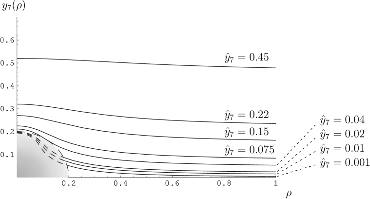
Figure 7: Embedding in the $y_{7}$ direction. The grey area corresponds to $r\leq mR^{2}$, into which also the shell of dielectric $\text{D}3$-branes present in the background is expected to expand ($R=1$ for the radius, $m=0.2$ for the adjoint masses, the dimensionless boundary value $\hat{y}_{4}$ determines the dimensionful quark mass $m_{\text{q}}$ according to $m_{\text{q}}=\frac{R}{2\pi\alpha^{\prime}}\hat{y}_{4}$).

Figure 7 shows that the $\text{D}7$-brane probes remain outside the shell for large values of the quark mass. For very small values of $m_{\text{q}}<0.04$, the approximation of the background metric to order $m^{2}$ in the adjoint masses breaks down: The embeddings are no longer monotonic functions of $r^{2}=\rho^{2}+y^{2}$ for $r<mR^{2}$.

Following the discussion of section 2.3, we expect the brane shell originating from the polarization of the background to expand into the $y_{7}$ direction. From the original probe calculation of [21], we expect the radius of the shell to be $r_{0}\sim kmR^{2}$, of the same order as our expansion parameter $mR^{2}$. $k$ is a number of order one related to the flux of $F_{2}$ on the $\text{D}7$ probe through the $S_{2}$ wrapped by the $\text{D}7$. A definite statement about the repulsion of the $\text{D}7$ probe by the shell in the background appears to be difficult since the shell is expected to be of the same size as our expansion parameter. Nevertheless, our result as displayed in figure 7 provides at least an indication that for small values of $m_{\text{q}}$, the $\text{D}7$ probes embedded in the $y_{7}$ direction merge with the background shell of polarized $\text{D}3$-branes at $r_{0}\sim mR^{2}=0.2$. This is supported further by the comparison with the embeddings in the $y^{4}$ direction, in which the shell does not form, as shown in figure 6. Consider for instance the embeddings with boundary value $\hat{y}_{4}=0.04$ in both figures. We see that $y_{4}(\rho)$ with boundary value $\hat{y}_{4}=0.04$ in figure 6 takes values smaller than $mR^{2}=0.2$, whereas $y^{7}(\rho)$ with boundary value $\hat{y}_{7}=0.04$ as shown in figure 7 is bounded from below by $mR^{2}=0.2$ – in fact, this solution does not enter the region with $r<mR^{2}$.

5.2.1 Meson mass

Finally, let us discuss some aspects of meson masses in the ${\cal N}=2$ Polchinski-Strassler background, as obtained from small fluctuations about the embedding.

Let us first consider what is expected from field theory for the dependence of the meson mass on the quark mass. The contributions to the meson mass arise essentially from the VEV’s of those contributions to the Lagrangian which break the $U(1)$ symmetry [44]. In our case these contributions are

$${\cal L}_{\text{breaking}}=m^{2}\phi_{\text{a}}^{2}+m\bar{\psi}_{\text{a}}\psi_{\text{a}}+m_{\text{q}}\bar{\psi}_{\text{f}}\psi_{\text{f}}+m_{\text{q}}^{2}\phi_{\text{f}}^{2}\leavevmode\nobreak\ ,$$ (5.5)

where ‘a’ stands for adjoint and ‘f’ for fundamental. Within QCD, $M^{2}\propto\langle{\cal L}_{\text{breaking}}\rangle$ implies the famous Gell-Mann-Oakes-Renner relation [45]. However in our case, VEV’s for fermion bilinears are forbidden by supersymmetry (they are F terms of a chiral multiplet and a non-vanishing VEV would imply that the vacuum is not SUSY invariant). Therefore, only scalar VEV’s may contribute to the meson mass and we have $M^{2}=b\,m^{2}+c\,m_{\text{q}}^{2}$, with $b$, $c$ some constants.

For the supergravity computation of the meson spectrum, we consider – as an example – radial fluctuations around the solution $y_{7}=y_{7}(\rho)$, $y_{4}=0$ of the form

$$\delta y^{7}(\rho,x)=\sin(k\cdot x)h(\rho)\leavevmode\nobreak\ ,\qquad M^{2}=-k^{2}\leavevmode\nobreak\ .$$ (5.6)

We insert the ansatz (5.6) into the action (5.1) and obtain the equations of motion linearized in $h$. The values for $M$ for which the solution is regular correspond to the meson masses. The result of this computation for the lowest-lying meson mode is plotted in figure 8.

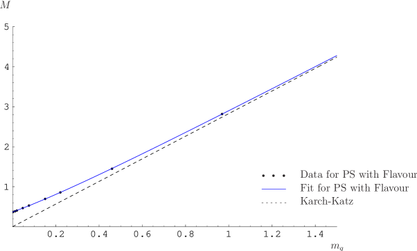
Figure 8: $y_{7}$ embedding: Meson mass in terms of quark mass $m_{\text{q}}$ (measured in units of $\frac{R}{2\pi\alpha^{\prime}}$) for adjoint mass $m=0.2$.

The spectrum shows a mass gap and is in agreement with the behaviour $M=\sqrt{c\,m_{\text{q}}^{2}+b\,m^{2}}$ expected from field theory, at least for $m_{\text{q}}\geq 0.04$ (the quark masses $m_{\text{q}}$ are given in units of $\frac{R}{2\pi\alpha^{\prime}}$). Note that due to our approximation of the gravity background to second order in the adjoint masses, the meson mass calculation breaks down for $m_{\text{q}}<0.04$, where the embeddings become unphysical, as may be seen from figure 7. For large values of $m_{\text{q}}$, the meson mass approaches the AdS result $M\propto m_{\text{q}}$. It is also instructive to plot the square of the meson mass versus the square of the quark mass. This is done in figure 9.

Figure 9: Square of the meson mass of figure 8 in terms of the square of the quark mass $m_{\text{q}}$ (measured in units of $\frac{R}{2\pi\alpha^{\prime}}$) for adjoint mass $m=0.2$.

For $m_{\text{q}}\geq 0.04$ this shows the expected linear behaviour, and for $m_{\text{q}}<0.04$ the expected breakdown of our approximation, which is already seen for the embedding in figure 7.

A detailed analysis of the meson spectra for both radial and angular fluctuations around both possible embeddings is beyond the scope of this paper. Due to the fact that the $U(1)$ symmetry in the two directions perpendicular to the $\text{D}7$ probe is broken already by the background, not just by the brane embedding itself, there may potentially be a mixing of $\delta y^{4}$ and $\delta y^{7}$ fluctuations. We leave a detailed study of the meson spectrum for the future.

6 Conclusions

By embedding a $\text{D}7$-brane probe into the ${\cal N}=2$ Polchinski-Strassler background, we have provided a model of holography with flavour – involving $\text{D}7$-brane probes in a non-conformal background – which is well under control both in the ultraviolet and in the infrared. In particular since the background itself forms a $\text{D}7$-like structure in the infrared via the blow-up of $\text{D}3$-branes, adding flavour via $\text{D}7$-brane probes appears to be natural. Our embeddings preserve the supersymmetry of the background. The meson mass displays a mass gap reflecting the presence of the adjoint masses, in agreement with field theory expectations.

These appealing physical interpretations are encouraging in view of generalizations of our results. It appears to be feasible to embed a $\text{D}7$-brane probe also in the standard ${\cal N}=1$ Polchinski-Strassler background [47]. Moreover from the view of applications to strongly coupled non-supersymmetric gauge theories it would be very interesting to consider the ${\cal N}=0$ background where also the gauginos acquire a mass [48]. Moreover, as mentioned in the introduction, for the ${\cal N}=2$ case there is the possibility of inducing spontaneous supersymmetry breaking via non-commutative instanton solutions on the $\text{D}7$-brane probe.

From a mathematical viewpoint, it would be interesting to investigate our embeddings using $\kappa$ symmetry in order to confirm the choice of sign of the Chern-Simons contribution to the action in (4.3). A further avenue is to investigate the holonomy and spinor structure along the lines of [25, 49, 50]. Moreover, it would be interesting to study how the Donagi-Witten field theory [29] in the infrared is modified by the presence of the $\text{D}7$-brane probe. A further interesting avenue is to make contact with model building [51].

We conclude that embedding $\text{D}7$-brane probes into the Polchinski-Strassler background is a promising approach for studying holography with flavour both conceptionally and in view of applications.

Appendix A Notation and conventions

The Hodge duality operator $\star_{d}$ maps an $r$-form $\omega_{r}$ to a $(d-r)$-form $\star_{d}\omega_{r}$. The latter has the components

$$\star_{d}\omega_{a_{1}\dots a_{d-r}}=\frac{\sqrt{|\det g_{ab}|}}{r!}\epsilon_{a_{1}\dots a_{d-r}}^{\hphantom{a_{1}\dots a_{d-r}}b_{1}\dots b_{r}}\omega_{b_{1}\dots b_{r}}\leavevmode\nobreak\ ,$$ (A.1)

where we have defined

$$\epsilon_{12\dots d}=1\leavevmode\nobreak\ .$$ (A.2)

The wedge product of an $r$-form $\omega_{r}$ and a $(d-r)$-form $\lambda_{d-r}$ in a $d$-dimensional space $\Sigma^{d}$ with metric $g_{ab}$ with $\tau$ negative eigenvalues and volume form

$$\operatorname{d}\!\operatorname{vol}(\Sigma^{d})=\sqrt{|\det g_{ab}|}\operatorname{d}\!^{d}\xi$$ (A.3)

reads

$$\omega_{r}\wedge\lambda_{d-r} =\omega_{r}\cdot(\star_{d}\lambda)_{r}\operatorname{d}\!\operatorname{vol}(\Sigma^{d})\leavevmode\nobreak\ ,\qquad\star_{d}^{2}=(-1)^{r(d-r)+\tau}\leavevmode\nobreak\ .$$ (A.4)

The inner product of two $r$-forms $\omega_{r}$ and $\omega^{\prime}_{r}$ is thereby defined as

$$\omega_{r}\cdot\omega^{\prime}_{r}=\frac{1}{r!}g^{a_{1}b_{1}}\dots g^{a_{r}b_{r}}\omega_{a_{1}\dots a_{r}}\omega^{\prime}_{b_{1}\dots b_{r}}\leavevmode\nobreak\ .$$ (A.5)

The components of the Hodge dual of an $r$-form are given in (A.1). The wedge product therefore becomes

$$\omega_{r}\wedge\lambda_{d-r} =\frac{\det g_{ab}}{r!(d-r)!}\epsilon^{a_{1}\dots a_{r}c_{1}\dots c_{d-r}}\omega_{a_{1}\dots a_{r}}\lambda_{c_{1}\dots c_{d-r}}\operatorname{d}\!\xi^{d}$$ (A.6)

$$=\frac{1}{r!(d-r)!}\epsilon_{a_{1}\dots a_{r}c_{1}\dots c_{d-r}}\omega_{a_{1}\dots a_{r}}\lambda_{c_{1}\dots c_{d-r}}\operatorname{d}\!\xi^{d}\leavevmode\nobreak\ ,$$

where in the last equality the independence of the wedge product of the (curved) metric has been used such that there the summation is understood as in flat space.

In type II B supergravity the physical field strengths are defined as

$$\tilde{F}_{r}=\operatorname{d}\!C_{r-1}-\operatorname{d}\!B\wedge C_{r-3}\leavevmode\nobreak\ ,\qquad r=1,3,5\leavevmode\nobreak\ ,$$ (A.7)

where for $r=1$ the second term is zero. The missing forms of higher degree ($r=7,9$) are found by applying the $(D=10)$-dimensional Hodge duality operator $\star=\star_{10}$

$$\tilde{F}_{9}=\star_{\mathrm{S}}\tilde{F}_{1}\leavevmode\nobreak\ ,\qquad\tilde{F}_{7}=-\star_{\mathrm{S}}\tilde{F}_{3}\leavevmode\nobreak\ ,\qquad\tilde{F}_{5}=\star_{\mathrm{S}}\tilde{F}_{5}\leavevmode\nobreak\ ,$$ (A.8)

where the suffix S indicates the use of the string frame metric in the definition of the Hodge star operator (A.1).

$\tilde{F}_{5}$ is self dual. This is a particularity we have to take into account. Following the conventions of [24], the $5$-form field strength $\tilde{F}_{5}$ is derived from a redefined $4$-form potential $C_{4}$. We have to replace

$$C_{4}\to C_{4}+\frac{1}{2}B\wedge C_{2}\leavevmode\nobreak\ .$$ (A.9)

Inserting this into (A.7), one finds

$$\tilde{F}_{5}=\star\tilde{F}_{5}=F_{5}-\frac{1}{2}C_{2}\wedge H_{3}+\frac{1}{2}F_{3}\wedge B\leavevmode\nobreak\ .$$ (A.10)

The Hodge star operator in (A.8) is evaluated with the string frame metric. Defining the relation

$$g_{MN}^{\mathrm{E}}=\operatorname{e}^{-\frac{\phi-\hat{\phi}}{2}}g_{MN}^{\mathrm{S}}$$ (A.11)

between the metric in the Einstein and the string frame, the corresponding Hodge stars, acting on an $r$-form, are related via

$$\star_{\mathrm{E}}=\operatorname{e}^{\frac{\phi-\hat{\phi}}{2}(r-\frac{D}{2})}\star_{\mathrm{S}}\leavevmode\nobreak\ .$$ (A.12)

We will skip the suffix E, denoting the Einstein frame, since this is the frame in which we work in the paper.

The only equation of motion which we will need for our determination of $C_{8}$ is the one for the complex dilaton-axion $\tau$

$$\operatorname{d}\!\star\operatorname{d}\!\tau-\frac{1}{i\operatorname{Im}\tau}\operatorname{d}\!\tau\wedge\star\operatorname{d}\!\tau-\frac{\operatorname{e}^{\hat{\phi}}}{2i}G_{3}\wedge\star G_{3}=0\leavevmode\nobreak\ .$$ (A.13)

which with the covariant derivative $\mathcal{D}_{M}$ becomes in components

$$\mathcal{D}^{2}\tau-\frac{1}{i\operatorname{Im}\tau}\partial_{M}\tau\partial^{M}\tau-\frac{\operatorname{e}^{\hat{\phi}}}{2i}G_{3}\cdot G_{3} =0\leavevmode\nobreak\ .$$ (A.14)

Since also the corrections to the background respect the four-dimensional Lorentz invariance, the metric always remains block diagonal w.r.t. the four directions longitudinal and the six directions transverse to the $\text{D}3$-brane. All further fields also do not contain mixed components, and hence the ten-dimensional Hodge star w.r.t. the unperturbed metric (2.1) effectively decomposes as

$$\star(\operatorname{d}\!x^{i_{1}}\wedge\dots\wedge\operatorname{d}\!x^{i_{r}})=Z^{\frac{1-r}{2}}\star_{6}(\operatorname{d}\!x^{i_{1}}\wedge\dots\wedge\operatorname{d}\!x^{i_{r}})\wedge\operatorname{d}\!\operatorname{vol}(\mathds{R}^{1,3})\leavevmode\nobreak\ ,$$ (A.15)

where $\star_{6}$ is the six-dimensional Hodge star w.r.t. flat Euclidean space.

In the expressions for the embedding of the $\text{D}7$-brane one has to use the inner product and Hodge star defined w.r.t. the pullback quantities. $P[\delta]_{ab}$ denotes the pullback of the Kronecker delta and $P[\delta]^{ab}$ its inverse. For two $r$-forms $\omega_{r}$, $\lambda_{r}$ they are defined as

$$\omega_{r}\cdot\lambda_{r}=\frac{1}{r!}P[\delta]^{a_{1}b_{1}}\dots P[\delta]^{a_{r}b_{r}}\omega_{a_{1}\dots a_{r}}\lambda_{b_{1}\dots b_{r}}\leavevmode\nobreak\ ,$$ (A.16)

$${\star_{d}}\omega_{a_{1}\dots a_{d-r}}=\frac{\sqrt{\det P[\delta]_{ab}}}{r!}P[\delta]^{c_{1}b_{1}}\dots P[\delta]^{c_{r}b_{r}}\omega_{c_{1}\dots c_{r}}\epsilon_{b_{1}\dots b_{r}a_{1}\dots a_{d-r}}\leavevmode\nobreak\ .$$ (A.17)

The Kronecker delta arises from the metric (2.1) in the six directions $y^{i}$ perpendicular to the $\text{D}3$-branes.

Appendix B The complex basis

It is convenient to introduce a complex basis with coordinates $z^{p}$ and their complex conjugates $\bar{z}^{p}$, defined in (2.9) and given by

$$z^{p}=\frac{1}{\sqrt{2}}(y^{p+3}+iy^{p+6})\leavevmode\nobreak\ ,\qquad p=1,2,3\leavevmode\nobreak\ .$$ (B.1)

In particular, for $\delta_{ij}$ one has in the complex basis

$$\delta_{p\bar{q}}=\delta_{\bar{p}q}=\begin{cases}1&p=q\\ 0&p\neq q\end{cases}\leavevmode\nobreak\ ,\qquad\delta_{pq}=0\leavevmode\nobreak\ .$$ (B.2)

A complex $2$-form can be written as

$$\omega_{2} =\frac{1}{2}\omega_{pq}\operatorname{d}\!z^{p}\wedge\operatorname{d}\!z^{q}+\omega_{p\bar{q}}\operatorname{d}\!z^{p}\wedge\operatorname{d}\!\bar{z}^{q}+\frac{1}{2}\omega_{\bar{p}\bar{q}}\operatorname{d}\!\bar{z}^{p}\wedge\operatorname{d}\!\bar{z}^{q}\leavevmode\nobreak\ ,$$ (B.3)

where we have used $\omega_{p\bar{q}}=-\omega_{\bar{q}p}$. The components of its complex conjugate fulfill

$$\bar{\omega}_{pq}=\overline{\omega_{\bar{p}\bar{q}}}\leavevmode\nobreak\ ,\qquad\bar{\omega}_{p\bar{q}}=\overline{\omega_{\bar{p}q}}\leavevmode\nobreak\ ,\qquad\bar{\omega}_{\bar{p}\bar{q}}=\overline{\omega_{pq}}\leavevmode\nobreak\ .$$ (B.4)

Subtracting and adding to $\omega_{2}$ its complex conjugate, one finds

$$\omega\pm\bar{\omega}_{2} =\frac{1}{2}(\omega_{pq}\pm\overline{\omega_{\bar{p}\bar{q}}})\operatorname{d}\!z^{p}\wedge\operatorname{d}\!z^{q}+(\omega_{p\bar{q}}\pm\overline{\omega_{\bar{p}q}})\operatorname{d}\!z^{p}\wedge\operatorname{d}\!\bar{z}^{q}+\frac{1}{2}(\omega_{\bar{p}\bar{q}}\pm\overline{\omega_{pq}})\operatorname{d}\!\bar{z}^{p}\wedge\operatorname{d}\!\bar{z}^{q}\leavevmode\nobreak\ .$$ (B.5)

The real and imaginary part of $\omega_{2}$ in the complex basis (2.9) are then found to be

$$\begin{aligned} \operatorname{Re}\omega_{pq}&=\frac{1}{2}(\omega_{pq}+\overline{\omega_{\bar{p}\bar{q}}})\leavevmode\nobreak\ ,\\ \operatorname{Re}\omega_{p\bar{q}}&=\frac{1}{2}(\omega_{p\bar{q}}+\overline{\omega_{\bar{p}q}})\leavevmode\nobreak\ ,\\ \operatorname{Re}\omega_{\bar{p}q}&=-\frac{1}{2}(\omega_{q\bar{p}}+\overline{\omega_{\bar{q}p}})\leavevmode\nobreak\ ,\\ \operatorname{Re}\omega_{\bar{p}\bar{q}}&=\frac{1}{2}(\omega_{\bar{p}\bar{q}}+\overline{\omega_{pq}})\leavevmode\nobreak\ ,\end{aligned}\qquad\begin{aligned} \operatorname{Im}\omega_{pq}&=-\frac{i}{2}(\omega_{pq}-\overline{\omega_{\bar{p}\bar{q}}})\leavevmode\nobreak\ ,\\ \operatorname{Im}\omega_{p\bar{q}}&=-\frac{i}{2}(\omega_{p\bar{q}}-\overline{\omega_{\bar{p}q}})\leavevmode\nobreak\ ,\\ \operatorname{Im}\omega_{\bar{p}q}&=\frac{i}{2}(\omega_{q\bar{p}}-\overline{\omega_{\bar{q}p}})\leavevmode\nobreak\ ,\\ \operatorname{Im}\omega_{\bar{p}\bar{q}}&=-\frac{i}{2}(\omega_{\bar{p}\bar{q}}-\overline{\omega_{pq}})\leavevmode\nobreak\ .\end{aligned}$$ (B.6)

In the complex basis (2.9) the inner product of two $2$-forms reads

$$\omega_{2}\cdot\omega^{\prime}_{2}=\frac{1}{2}(\omega_{pq}\omega^{\prime}_{\bar{p}\bar{q}}+\omega_{\bar{p}\bar{q}}\omega^{\prime}_{pq})+\omega_{p\bar{q}}\omega^{\prime}_{\bar{p}q}\leavevmode\nobreak\ ,$$ (B.7)

where summation over repeated indices is understood.

With the convention $\epsilon_{456789}=1$ in the real basis, the non-vanishing components of the six-dimensional total antisymmetric tensor density in the complex basis are given by

$$\epsilon_{123\bar{1}\bar{2}\bar{3}}=-i$$ (B.8)

and permutations thereof. A general component can then be represented as

$$\epsilon_{pqr\bar{s}\bar{t}\bar{u}}=-i\epsilon_{pqr}\epsilon_{\bar{s}\bar{t}\bar{u}}=-i\big{(}(\delta_{p\bar{s}}\delta_{q\bar{t}}-\delta_{p\bar{t}}\delta_{q\bar{s}})\delta_{r\bar{u}}+(\delta_{p\bar{t}}\delta_{q\bar{u}}-\delta_{p\bar{u}}\delta_{q\bar{t}})\delta_{r\bar{s}}+(\delta_{p\bar{u}}\delta_{q\bar{s}}-\delta_{p\bar{s}}\delta_{q\bar{u}})\delta_{r\bar{t}}\big{)}\leavevmode\nobreak\ .$$ (B.9)

Here a warning has to be made. The above representation in that form is valid only for the given order of unbared and bared components, since the r.h.r. is not totally antisymmetric under permutations of bared and unbared indices. In the generic case one has to adjust the global sign of the r.h.s. to take care of the order. For example, interchanging $r$ and $\bar{s}$ yields

$$\epsilon_{pq\bar{s}r\bar{t}\bar{u}}=i\epsilon_{pqr}\epsilon_{\bar{s}\bar{t}\bar{u}}=i\big{(}(\delta_{p\bar{s}}\delta_{q\bar{t}}-\delta_{p\bar{t}}\delta_{q\bar{s}})\delta_{ru}+(\delta_{p\bar{t}}\delta_{q\bar{u}}-\delta_{p\bar{u}}\delta_{q\bar{t}})\delta_{r\bar{s}}+(\delta_{p\bar{u}}\delta_{q\bar{s}}-\delta_{p\bar{s}}\delta_{q\bar{u}})\delta_{r\bar{t}}\big{)}\leavevmode\nobreak\ .$$ (B.10)

An embedding of a $\text{D}7$-brane along $z^{a}$, $z^{b}$, $\bar{z}^{a}$, $\bar{z}^{b}$, $a,b=2,3$ and perpendicular to $z^{m}$, $\bar{z}^{m}$, $m=1$ induces a four-dimensional total antisymmetric tensor density on the parallel four directions. One obtains from (B.9) for the six-dimensional tensor density

$$\epsilon_{mab\bar{m}\bar{c}\bar{d}}=-i\epsilon_{mab}\epsilon_{\bar{m}\bar{c}\bar{d}}=-i(\delta_{a\bar{c}}\delta_{b\bar{d}}-\delta_{a\bar{d}}\delta_{b\bar{c}})\leavevmode\nobreak\ .$$ (B.11)

The four-dimensional $\epsilon$ tensor then reads

$$\epsilon_{ab\bar{c}\bar{d}}=-\epsilon_{a\bar{c}b\bar{d}}=-i\epsilon_{mab\bar{m}\bar{c}\bar{d}}=-\epsilon_{mab}\epsilon_{\bar{m}\bar{c}\bar{d}}=-\delta_{a\bar{c}}\delta_{b\bar{d}}+\delta_{a\bar{d}}\delta_{b\bar{c}}\leavevmode\nobreak\ ,$$ (B.12)

where the factor $i$ is chosen to ensure that in real coordinates the four-dimensional $\epsilon$ tensor is normalized to $1$. With the above results, a four-dimensional Hodge star operator on the parallel four directions is defined. Using the representation (B.12), one finds that $\star_{4}$ acts on a $2$-form $\omega_{2}$ as follows

$$\star_{4}\omega_{ab}=-\omega_{ab}\leavevmode\nobreak\ ,\qquad\star_{4}\omega_{a\bar{b}}=\omega_{a\bar{b}}-\delta_{a\bar{b}}\omega_{c\bar{c}}\leavevmode\nobreak\ ,\qquad\star_{4}\omega_{\bar{a}b}=\omega_{\bar{a}b}-\delta_{a\bar{b}}\omega_{\bar{c}c}\leavevmode\nobreak\ ,\qquad\star_{4}\omega_{\bar{a}\bar{b}}=-\omega_{\bar{a}\bar{b}}\leavevmode\nobreak\ ,$$ (B.13)

where a summation over $c$ is understood. The above relations act differently on the components of $\omega_{2}$ which are parallel to purely (anti)holomorphic directions and which point in mixed directions. A generic $2$-form $\omega_{2}$ behaves as

$$\frac{1}{2}(1-\star_{4})\omega_{2}=\omega_{(2,0)}+\omega_{(0,2)}-\frac{i}{2}\omega_{c\bar{c}}K\leavevmode\nobreak\ ,\qquad\frac{1}{2}(1+\star_{4})\omega_{2}=\omega_{(1,1)}^{\text{P}}\leavevmode\nobreak\ ,$$ (B.14)

where P denotes the primitive part of $\omega_{2}$, i.e. $\omega_{2}^{\text{P}}\cdot K=0$ and

$$K=i\delta_{a\bar{b}}\operatorname{d}\!z^{a}\wedge\operatorname{d}\!\bar{z}^{b}$$ (B.15)

is the Kähler form of the flat four-dimensional space. A general linear combination with $\star_{4}$ then acts as

$$(\alpha-\beta\star_{4})\omega_{2}=(\alpha+\beta)\Big{(}\omega_{(2,0)}+\omega_{(0,2)}-\frac{i}{2}\omega_{c\bar{c}}K\Big{)}+(\alpha-\beta)\omega_{(1,1)}^{\text{P}}\leavevmode\nobreak\ .$$ (B.16)

In the complex basis the exterior derivative operator $\operatorname{d}\!$ splits into its holomorphic and antiholomorphic derivative $\partial$ and $\bar{\partial}$, respectively

$$\operatorname{d}\!=\partial+\bar{\partial}\leavevmode\nobreak\ .$$ (B.17)

The nilpotency of $\operatorname{d}\!$ translates into the relations

$$\partial^{2}=\bar{\partial}^{2}=0\leavevmode\nobreak\ ,\qquad\partial\bar{\partial}=-\bar{\partial}\partial\leavevmode\nobreak\ .$$ (B.18)

The components of the tensor $T_{3}$ (2.11) in the real basis read

$$T_{p+3\,q+3\,r+3} =\phantom{-}\frac{1}{2\sqrt{2}}\epsilon_{pqr}(m_{1}+m_{2}+m_{3})=\phantom{-}iT_{p+6\,q+6\,r+6}\leavevmode\nobreak\ ,$$ (B.19)

$$T_{p+3\,q+3\,r+6} =-\frac{i}{2\sqrt{2}}\epsilon_{pqr}(m_{1}+m_{2}-m_{3})=-iT_{p+6\,q+6\,r+3}\leavevmode\nobreak\ ,$$

$$T_{p+3\,q+6\,r+3} =-\frac{i}{2\sqrt{2}}\epsilon_{pqr}(m_{1}-m_{2}+m_{3})=-iT_{p+6\,q+3\,r+6}\leavevmode\nobreak\ ,$$

$$T_{p+6\,q+3\,r+3} =\phantom{-}\frac{i}{2\sqrt{2}}\epsilon_{pqr}(m_{1}-m_{2}-m_{3})=-iT_{p+3\,q+6\,r+6}\leavevmode\nobreak\ .$$

The $2$-form $S_{2}$ as defined in (2.8) reads

$$S_{2} =\frac{1}{2}\epsilon_{pqr}(m_{p}z^{p}\operatorname{d}\!\bar{z}^{q}\wedge\operatorname{d}\!\bar{z}^{r}+m_{q}\bar{z}^{p}\operatorname{d}\!z^{q}\wedge\operatorname{d}\!\bar{z}^{r}+m_{r}\bar{z}^{p}\operatorname{d}\!\bar{z}^{q}\wedge\operatorname{d}\!z^{r})$$ (B.20)

$$=\frac{1}{2}\epsilon_{pqr}(m_{p}z^{p}\operatorname{d}\!\bar{z}^{q}+2m_{q}\bar{z}^{p}\operatorname{d}\!z^{q})\wedge\operatorname{d}\!\bar{z}^{r}\leavevmode\nobreak\ .$$

One finds from (B.20) that the components of $S_{2}$ are given by

$$S_{p\bar{q}}=\epsilon_{rpq}m_{p}\bar{z}^{r}\leavevmode\nobreak\ ,\qquad S_{\bar{p}q}=\epsilon_{rpq}m_{q}\bar{z}^{r}\leavevmode\nobreak\ ,\qquad S_{\bar{p}\bar{q}}=\epsilon_{rpq}m_{r}z^{r}\leavevmode\nobreak\ .$$ (B.21)

The components of the real and imaginary parts then read

$$\begin{aligned} \operatorname{Re}S_{pq}&=\frac{1}{2}\epsilon_{rpq}m_{r}\bar{z}^{r}\leavevmode\nobreak\ ,\\ \operatorname{Re}S_{p\bar{q}}&=\frac{1}{2}\epsilon_{rpq}(m_{p}\bar{z}^{r}+m_{q}z^{r})\leavevmode\nobreak\ ,\\ \operatorname{Re}S_{\bar{p}q}&=\frac{1}{2}\epsilon_{rpq}(m_{q}\bar{z}^{r}+m_{p}z^{r})\leavevmode\nobreak\ ,\\ \operatorname{Re}S_{\bar{p}\bar{q}}&=\frac{1}{2}\epsilon_{rpq}m_{r}z^{r}\leavevmode\nobreak\ ,\end{aligned}\qquad\begin{aligned} \operatorname{Im}S_{pq}&=\frac{i}{2}\epsilon_{rpq}m_{r}\bar{z}^{r}\leavevmode\nobreak\ ,\\ \operatorname{Im}S_{p\bar{q}}&=-\frac{i}{2}\epsilon_{rpq}(m_{p}\bar{z}^{r}-m_{q}z^{r})\leavevmode\nobreak\ ,\\ \operatorname{Im}S_{\bar{p}q}&=-\frac{i}{2}\epsilon_{rpq}(m_{q}\bar{z}^{r}-m_{p}z^{r})\leavevmode\nobreak\ ,\\ \operatorname{Im}S_{\bar{p}\bar{q}}&=-\frac{i}{2}\epsilon_{rpq}m_{r}z^{r}\leavevmode\nobreak\ ,\end{aligned}$$ (B.22)

where $p$, $q$ are not summed over. It is easily checked that the real and imaginary parts with mixed components are consistent with the antisymmetry of $S_{2}$.

Taking into account the split of the coordinates according to the presence of a $\text{D}7$-brane, the complex $2$-form $S_{2}$ as given in (B.20) decomposes in terms of the coordinates $z^{a}$, $z^{b}$, $\bar{z}^{a}$, $\bar{z}^{b}$ and $z^{m}$, $\bar{z}^{m}$ along and transverse to the $\text{D}7$-brane as

$$S_{2} =S_{2}^{\parallel}+S_{2}^{\text{mixed}}\leavevmode\nobreak\ ,$$ (B.23)

$$S_{2}^{\parallel} =\frac{1}{2}\big{(}T_{m\bar{a}\bar{b}}z^{m}\operatorname{d}\!\bar{z}^{a}\wedge\operatorname{d}\!\bar{z}^{b}+2T_{\bar{m}a\bar{b}}\bar{z}^{m}\operatorname{d}\!z^{a}\wedge\operatorname{d}\!\bar{z}^{b}\big{)}\leavevmode\nobreak\ ,$$

$$S_{2}^{\text{mixed}} =T_{b\bar{a}\bar{m}}z^{b}\operatorname{d}\!\bar{z}^{a}\wedge\operatorname{d}\!\bar{z}^{m}+T_{\bar{b}a\bar{m}}\bar{z}^{b}\operatorname{d}\!z^{a}\wedge\operatorname{d}\!\bar{z}^{m}+T_{\bar{b}m\bar{a}}\bar{z}^{b}\operatorname{d}\!z^{m}\wedge\operatorname{d}\!\bar{z}^{a}\leavevmode\nobreak\ ,$$

where the components in purely transverse directions vanish. We have restored the $3$-tensor $T_{3}$ according to (2.8). This is convenient for a later identification of the individual contributions in terms of the $2$-form potentials. The pullback into the four directions $z^{a}$, $z^{b}$, $\bar{z}^{a}$, $\bar{z}^{b}$ can be recast as follows

$$P[S_{2}] =\frac{3}{2}T_{m\bar{a}\bar{b}}z^{m}\operatorname{d}\!\bar{z}^{a}\wedge\operatorname{d}\!\bar{z}^{b}+3T_{\bar{m}a\bar{b}}\bar{z}^{m}\operatorname{d}\!z^{a}\wedge\operatorname{d}\!\bar{z}^{b}$$ (B.24)

$$\phantom{{}={}}-(\partial+\bar{\partial})(T_{m\bar{a}\bar{b}}z^{m}\bar{z}^{a}\operatorname{d}\!\bar{z}^{b}+T_{\bar{m}a\bar{b}}\bar{z}^{m}z^{a}\operatorname{d}\!\bar{z}^{b}+T_{\bar{m}\bar{a}b}\bar{z}^{m}\bar{z}^{a}\operatorname{d}\!z^{b})\leavevmode\nobreak\ ,$$

where $\partial$, $\bar{\partial}$ act along the four parallel directions. We have rearranged some terms to complete exterior derivatives, which will turn out to be useful in the following. The imaginary part of the above expression then decomposes into its holomorphic and antiholomorphic components as follows

$$P[\operatorname{Im}S_{2}]_{(2,0)} =i\frac{3}{2}\bar{S}_{(2,0)}^{\parallel}-\frac{i}{2}\partial\theta=3\operatorname{Im}S_{(2,0)}^{\parallel}-\frac{i}{2}\partial\theta\leavevmode\nobreak\ ,$$ (B.25)

$$P[\operatorname{Im}S_{2}]_{(1,1)} =-i\frac{3}{2}(S_{(1,1)}^{\parallel}-\bar{S}_{(1,1)}^{\parallel})-\frac{i}{2}(\bar{\partial}\theta-\partial\bar{\theta})=3\operatorname{Im}S_{(1,1)}^{\parallel}-\frac{i}{2}(\bar{\partial}\theta-\partial\bar{\theta})\leavevmode\nobreak\ ,$$

$$P[\operatorname{Im}S_{2}]_{(0,2)} =-i\frac{3}{2}S_{(0,2)}^{\parallel}+\frac{i}{2}\bar{\partial}\bar{\theta}=3\operatorname{Im}S_{(0,2)}^{\parallel}+\frac{i}{2}\bar{\partial}\bar{\theta}\leavevmode\nobreak\ .$$

We have thereby made use of the definition of the parallel components in (B.23), as well as of the results $S_{(2,0)}=0$ and $\bar{S}_{(0,2)}=0$. The $1$-form $\theta$ that appears above is defined as

$$\theta=\theta_{(1,0)} =(\bar{T}_{m\bar{a}b}\bar{z}^{a}z^{m}+\bar{T}_{\bar{m}ab}z^{a}\bar{z}^{m}-T_{\bar{m}\bar{a}b}\bar{z}^{a}\bar{z}^{m})\operatorname{d}\!z^{b}\leavevmode\nobreak\ .$$ (B.26)

Inserting (B.22) into (2.13), one finds that the individual components of $\tilde{C}_{2}$ and $B$ in the complex basis are given by

$$\begin{aligned} \tilde{C}_{pq}&=\operatorname{e}^{-\hat{\phi}}\frac{\zeta}{6}Z\epsilon_{rpq}m_{r}\bar{z}^{r}\leavevmode\nobreak\ ,\\ \tilde{C}_{p\bar{q}}&=\operatorname{e}^{-\hat{\phi}}\frac{\zeta}{6}Z\epsilon_{rpq}(m_{p}\bar{z}^{r}+m_{q}z^{r})\leavevmode\nobreak\ ,\\ \tilde{C}_{\bar{p}q}&=\operatorname{e}^{-\hat{\phi}}\frac{\zeta}{6}Z\epsilon_{rpq}(m_{q}\bar{z}^{r}+m_{p}z^{r})\leavevmode\nobreak\ ,\\ \tilde{C}_{\bar{p}\bar{q}}&=\operatorname{e}^{-\hat{\phi}}\frac{\zeta}{6}Z\epsilon_{rpq}m_{r}z^{r}\leavevmode\nobreak\ ,\end{aligned}\qquad\begin{aligned} B_{pq}&=-i\frac{\zeta}{6}Z\epsilon_{rpq}m_{r}\bar{z}^{r}\leavevmode\nobreak\ ,\\ B_{p\bar{q}}&=i\frac{\zeta}{6}Z\epsilon_{rpq}(m_{p}\bar{z}^{r}-m_{q}z^{r})\leavevmode\nobreak\ ,\\ B_{\bar{p}q}&=i\frac{\zeta}{6}Z\epsilon_{rpq}(m_{q}\bar{z}^{r}-m_{p}z^{r})\leavevmode\nobreak\ ,\\ B_{\bar{p}\bar{q}}&=i\frac{\zeta}{6}Z\epsilon_{rpq}m_{r}z^{r}\leavevmode\nobreak\ .\end{aligned}$$ (B.27)

In the special case $m_{1}=0$, $m_{2}=m_{3}=m$, the inner products in four dimensions hence become

$$\tilde{C}_{2}\cdot\tilde{C}_{2} =\tilde{C}_{ab}\tilde{C}_{\bar{a}\bar{b}}+\tilde{C}_{a\bar{b}}\tilde{C}_{\bar{a}b}=\operatorname{e}^{-2\hat{\phi}}\frac{\zeta^{2}m^{2}}{18}Z^{2}(2z^{m}\bar{z}^{m}+z^{m}z^{m}+\bar{z}^{m}\bar{z}^{m})\leavevmode\nobreak\ ,$$ (B.28)

$$\tilde{C}_{2}\cdot B =\tilde{C}_{ab}B_{\bar{a}\bar{b}}+\tilde{C}_{\bar{a}\bar{b}}B_{ab}+\tilde{C}_{a\bar{b}}B_{\bar{a}b}+\tilde{C}_{b\bar{a}}B_{\bar{b}a}=-i\operatorname{e}^{-\hat{\phi}}\frac{\zeta^{2}m^{2}}{18}Z^{2}(z^{m}z^{m}-\bar{z}^{m}\bar{z}^{m})\leavevmode\nobreak\ ,$$

$$B\cdot B =B_{ab}B_{\bar{a}\bar{b}}+B_{a\bar{b}}B_{\bar{a}b}=\frac{\zeta^{2}m^{2}}{18}Z^{2}(2z^{m}\bar{z}^{m}-z^{m}z^{m}-\bar{z}^{m}\bar{z}^{m})\leavevmode\nobreak\ ,$$

and

$$\tilde{C}_{2}\cdot\star_{4}\tilde{C}_{2} =-\tilde{C}_{ab}\tilde{C}_{\bar{a}\bar{b}}+\tilde{C}_{a\bar{a}}\tilde{C}_{b\bar{b}}+\tilde{C}_{a\bar{b}}\tilde{C}_{\bar{a}b}=\operatorname{e}^{-2\hat{\phi}}\frac{\zeta^{2}m^{2}}{18}Z^{2}(2z^{m}\bar{z}^{m}+z^{m}z^{m}+\bar{z}^{m}\bar{z}^{m})\leavevmode\nobreak\ ,$$ (B.29)

$$\tilde{C}_{2}\cdot\star_{4}B =-\frac{1}{2}(\tilde{C}_{ab}B_{\bar{a}\bar{b}}+\tilde{C}_{\bar{a}\bar{b}}B_{ab})+\tilde{C}_{a\bar{a}}B_{b\bar{b}}+\tilde{C}_{a\bar{b}}B_{\bar{a}b}=i\operatorname{e}^{-\hat{\phi}}\frac{\zeta^{2}m^{2}}{18}Z^{2}(z^{m}z^{m}-\bar{z}^{m}\bar{z}^{m})\leavevmode\nobreak\ ,$$

$$B\cdot\star_{4}B =-B_{ab}B_{\bar{a}\bar{b}}+B_{a\bar{a}}B_{b\bar{b}}+B_{a\bar{b}}B_{\bar{a}b}=\frac{\zeta^{2}m^{2}}{18}Z^{2}(2z^{m}\bar{z}^{m}-z^{m}z^{m}-\bar{z}^{m}\bar{z}^{m})\leavevmode\nobreak\ .$$

A combination that appears in the equations of motion for the embedding is then determined as

$$\frac{1}{2}Z^{-1}\Big{(}1-\frac{2}{3}\star_{4}\Big{)}B\cdot B-\frac{1}{6}\operatorname{e}^{2\hat{\phi}}Z^{-1}\star_{4}\tilde{C}_{2}\cdot\tilde{C}_{2}=-\frac{\zeta^{2}m^{2}}{54}Z(z^{m}z^{m}+\bar{z}^{m}\bar{z}^{m})\leavevmode\nobreak\ ,$$ (B.30)

where $\star_{4}$ is understood to act on the first form on its right.

Furthermore, one needs similar expressions where not all components are summed. They read

$$\frac{Z^{-1}}{3}\big{(}(1-4\star_{4})(B_{ab}B_{m\bar{b}}+B_{a\bar{b}}B_{mb})-\operatorname{e}^{2\hat{\phi}}\star_{4}(\tilde{C}_{ab}\tilde{C}_{m\bar{b}}+\tilde{C}_{a\bar{b}}\tilde{C}_{mb})\big{)}=\frac{\zeta^{2}m^{2}}{54}Z(2\bar{z}^{a}\bar{z}^{m}-\bar{z}^{a}z^{m})\leavevmode\nobreak\ ,$$ (B.31)

$$\frac{Z^{-1}}{3}\big{(}(1-4\star_{4})(B_{\bar{a}b}B_{m\bar{b}}+B_{\bar{a}\bar{b}}B_{mb})-\operatorname{e}^{2\hat{\phi}}\star_{4}(\tilde{C}_{\bar{a}b}\tilde{C}_{m\bar{b}}+\tilde{C}_{\bar{a}\bar{b}}\tilde{C}_{mb})\big{)}=\frac{\zeta^{2}m^{2}}{54}Z(2z^{a}\bar{z}^{m}-z^{a}z^{m})\leavevmode\nobreak\ ,$$

where on the l.h.s. a sum over $b$ is understood, and $a$, $m$ take fixed values. One thereby first has to act with $\star_{4}$ on the right and then extract the required components

The correction to the dilaton decomposes as

$$\tilde{\phi}=\varphi Y_{+}\leavevmode\nobreak\ ,$$ (B.32)

where $\varphi=\varphi(r)$, and the spherical harmonic $Y_{+}$ arises as the real part of the expression

$$T_{ijk}V_{ijk} =V_{ijk}V_{ijk}=\frac{3}{r^{2}}y^{i}y^{l}T_{ijk}T_{ljk}=2M^{2}(Y_{+}-Y_{-})\leavevmode\nobreak\ ,$$ (B.33)

where $M^{2}$ is defined as the sum of the squares of all masses as in (2.18). The tensor $V_{ijk}$ is defined in [21], and for generic masses $Y_{\pm}$ are $SO(6)$ spherical harmonics with eigenvalue $-\frac{12}{R^{2}}$ which are explicitly given by

$$Y_{\pm}=\frac{3}{M^{2}r^{2}}\big{(}m_{2}m_{3}(z^{1}z^{1}\pm\bar{z}^{1}\bar{z}^{1})+m_{1}m_{3}(z^{2}z^{2}\pm\bar{z}^{2}\bar{z}^{2})+m_{1}m_{2}(z^{3}z^{3}\pm\bar{z}^{3}\bar{z}^{3})\big{)}\leavevmode\nobreak\ .$$ (B.34)

The above tensor contraction appears on the r.h.s. in the equation of motion (A.14) for the complex dilation-axion $\tau$.

$$G_{3}\cdot G_{3} =\frac{\zeta^{2}}{3!}Z^{\frac{1}{2}}\Big{(}T_{ijk}-\frac{4}{3}V_{ijk}\Big{)}\Big{(}T_{ijk}-\frac{4}{3}V_{ijk}\Big{)}=-\frac{4\zeta^{2}}{27}Z^{\frac{1}{2}}T_{ijk}V_{ijk}\leavevmode\nobreak\ .$$ (B.35)

With these results, it is easy to determine the radial dependent part in (B.32) as

$$\varphi=\frac{\zeta^{2}M^{2}R^{2}}{108}\hat{Z}^{\frac{1}{2}}\leavevmode\nobreak\ .$$ (B.36)

The tensors (2.17) for the corrected metric (2.16) read in complex coordinates

$$I_{pq}=-\frac{\bar{z}^{p}\bar{z}^{q}}{10z\bar{z}}\leavevmode\nobreak\ ,\qquad I_{p\bar{q}}=\frac{1}{5}\Big{(}\delta_{p\bar{q}}-\frac{\bar{z}^{p}z^{q}}{2z\bar{z}}\Big{)}\leavevmode\nobreak\ ,\qquad$$ (B.37)

and

$$W_{pq} =\frac{1}{4M^{2}z\bar{z}}(2\delta_{p\bar{q}}m_{p}m_{r}\bar{z}^{r}\bar{z}^{r}-(m_{p}^{2}+m_{q}^{2})\bar{z}^{p}\bar{z}^{q})+\frac{\bar{z}^{p}\bar{z}^{q}}{10z\bar{z}}\leavevmode\nobreak\ ,$$ (B.38)

$$W_{p\bar{q}} =\frac{1}{20}\Big{(}\delta_{p\bar{q}}-3\frac{\bar{z}^{p}z^{q}}{z\bar{z}}\Big{)}+\frac{1}{4M^{2}z\bar{z}}((m_{p}^{2}+m_{q}^{2})\bar{z}^{p}z^{q}-2m_{p}m_{q}z^{p}\bar{z}^{q})\leavevmode\nobreak\ .$$

The remaining components are obtained by complex conjugation from the above expressions. Taking the traces of the corrections in (2.16) w.r.t. to the four-dimensional subspace, i.e. summing over $a=2,3$, thereby using that

$$\rho^{2}=2z^{a}\bar{z}^{a}\leavevmode\nobreak\ ,\qquad u^{2}=2z^{m}\bar{z}^{m}\leavevmode\nobreak\ ,\qquad r^{2}=\rho^{2}+u^{2}\leavevmode\nobreak\ ,$$ (B.39)

one finds

$$\tilde{g}_{aa} =\frac{1}{10}(6p+10q-w)+\frac{u^{2}}{r^{2}}\frac{1}{10}(2p-10q+3w)\leavevmode\nobreak\ .$$ (B.40)

Furthermore, the required off-diagonal elements read

$$\tilde{g}_{am} =\frac{1}{10z\bar{z}}(5q-p+w)\bar{z}^{a}\bar{z}^{m}-\frac{w}{4M^{2}z\bar{z}}(m_{a}^{2}+m_{m}^{2})\bar{z}^{a}\bar{z}^{m}\leavevmode\nobreak\ ,$$ (B.41)

$$\tilde{g}_{\bar{a}m} =\frac{1}{20z\bar{z}}(10q-2p-3w)z^{a}\bar{z}^{m}+\frac{w}{4M^{2}z\bar{z}}((m_{a}^{2}+m_{m}^{2})z^{a}\bar{z}^{m}-2m_{a}m_{m}\bar{z}^{a}z^{m})\leavevmode\nobreak\ ,$$

where the missing combinations are obtained by complex conjugation. Furthermore, $m_{a}$ and $m_{m}$ indicate the masses corresponding to the direction $a=2,3$ and $m=1$ in the complex basis, respectively. No summation over $a$ and $m$ is understood on the r.h.s. In particular, we need the specialization to $m_{m}=0$ and $m_{a}=m$ independent of $a$.

Appendix C Form relations to compute $C_{8}$

We will work with generic masses in the following. This keeps the expressions compact and leads to a result which is valid beyond the special case analyzed in this paper. The determination of $C_{8}$ requires the explicit result for the wedge product of $S_{2}$ with its complex conjugate $\bar{S}_{2}$. Using the explicit expression (B.20) for $S_{2}$ and its complex conjugate, as well as the representation of the product of two $\epsilon$ tensors in terms of Kronecker $\delta$s similar to (B.9), the result can be recast into the form

$$S_{2}\wedge\bar{S}_{2} =-\frac{1}{2}(m_{p}m_{p}-2m_{q}m_{q})z^{p}\bar{z}^{p}\operatorname{d}\!z^{q}\wedge\operatorname{d}\!\bar{z}^{q}\wedge\operatorname{d}\!z^{r}\wedge\operatorname{d}\!\bar{z}^{r}$$ (C.1)

$$\phantom{={}}-\frac{1}{2}(m_{p}m_{p}-m_{q}m_{q})(z^{p}z^{q}\operatorname{d}\!\bar{z}^{q}\wedge\operatorname{d}\!\bar{z}^{p}-\bar{z}^{p}\bar{z}^{q}\operatorname{d}\!z^{q}\wedge\operatorname{d}\!z^{p})\wedge\operatorname{d}\!z^{r}\wedge\operatorname{d}\!\bar{z}^{r}$$

$$\phantom{={}}+m_{q}m_{q}\bar{z}^{p}z^{r}\operatorname{d}\!z^{q}\wedge\operatorname{d}\!\bar{z}^{q}\wedge\operatorname{d}\!\bar{z}^{r}\wedge\operatorname{d}\!z^{p}\leavevmode\nobreak\ .$$

Introducing the diagonal mass matrix and its square

$$M_{pq}=m_{p}\delta_{pq}\leavevmode\nobreak\ ,\qquad M^{2}_{pq}=M_{pr}M_{rq}=m_{p}^{2}\delta_{pq}\leavevmode\nobreak\ ,$$ (C.2)

one can rewrite (C.1) as

$$S_{2}\wedge\bar{S}_{2} =\Big{[}-\frac{1}{2}zM^{2}\bar{z}\operatorname{d}\!z\wedge\operatorname{d}\!\bar{z}+z\bar{z}\operatorname{d}\!z\overset{M^{2}}{\wedge}\operatorname{d}\!\bar{z}-z\operatorname{d}\!\bar{z}\wedge zM^{2}\operatorname{d}\!\bar{z}+\bar{z}\operatorname{d}\!z\wedge\bar{z}M^{2}\operatorname{d}\!z\Big{]}\wedge\operatorname{d}\!z\wedge\operatorname{d}\!\bar{z}$$ (C.3)

$$\phantom{={}}+\operatorname{d}\!z\overset{M^{2}}{\wedge}\operatorname{d}\!\bar{z}\wedge z\operatorname{d}\!\bar{z}\wedge\bar{z}\operatorname{d}\!z\leavevmode\nobreak\ .$$

The following abbreviations have thereby been used

$$\begin{gathered}z\bar{z}=z^{p}\bar{z}^{p}\leavevmode\nobreak\ ,\qquad zM^{2}\bar{z}=m_{p}^{2}z^{p}\bar{z}^{p}\leavevmode\nobreak\ ,\qquad\operatorname{d}\!z\wedge\operatorname{d}\!\bar{z}=\operatorname{d}\!z^{p}\wedge\operatorname{d}\!\bar{z}^{p}\leavevmode\nobreak\ ,\qquad\operatorname{d}\!z\overset{M^{2}}{\wedge}\operatorname{d}\!\bar{z}=m_{p}^{2}\operatorname{d}\!z^{p}\wedge\operatorname{d}\!\bar{z}^{p}\leavevmode\nobreak\ ,\\ z\operatorname{d}\!\bar{z}\wedge\bar{z}\operatorname{d}\!z=z^{p}\operatorname{d}\!\bar{z}^{p}\wedge\bar{z}^{q}\operatorname{d}\!z^{q}\leavevmode\nobreak\ ,\qquad z\operatorname{d}\!\bar{z}\wedge zM^{2}\operatorname{d}\!\bar{z}=m_{q}^{2}z^{p}\operatorname{d}\!\bar{z}^{p}\wedge z^{q}\operatorname{d}\!\bar{z}^{q}\leavevmode\nobreak\ ,\qquad\end{gathered}$$ (C.4)

where a summation over $p,q=1,2,3$ is understood on the r.h.s., and a similar abbreviation holds for the complex conjugate of the last expression. With the relations

$$z\operatorname{d}\!\bar{z}\wedge zM^{2}\operatorname{d}\!\bar{z} =\operatorname{d}\!(z\bar{z})\wedge zM^{2}\operatorname{d}\!\bar{z}-\bar{z}\operatorname{d}\!z\wedge\operatorname{d}\!(zM^{2}\bar{z})+\bar{z}\operatorname{d}\!z\wedge\bar{z}M^{2}\operatorname{d}\!z\leavevmode\nobreak\ ,$$ (C.5)

$$\bar{z}\operatorname{d}\!z\wedge\operatorname{d}\!(zM^{2}\bar{z}) =-\operatorname{d}\!(zM^{2}\bar{z}\bar{z}\operatorname{d}\!z)-zM^{2}\bar{z}\operatorname{d}\!z\wedge\operatorname{d}\!\bar{z}$$

the result can be rewritten as

$$S_{2}\wedge\bar{S}_{2} =\Big{[}-\frac{3}{2}zM^{2}\bar{z}\operatorname{d}\!z\wedge\operatorname{d}\!\bar{z}+z\bar{z}\operatorname{d}\!z\overset{M^{2}}{\wedge}\operatorname{d}\!\bar{z}-\operatorname{d}\!(z\bar{z})\wedge zM^{2}\operatorname{d}\!\bar{z}-\operatorname{d}\!(zM^{2}\bar{z}\bar{z}\operatorname{d}\!z)\Big{]}\wedge\operatorname{d}\!z\wedge\operatorname{d}\!\bar{z}$$ (C.6)

$$\phantom{={}}+\operatorname{d}\!z\overset{M^{2}}{\wedge}\operatorname{d}\!\bar{z}\wedge\operatorname{d}\!(z\bar{z})\wedge\bar{z}\operatorname{d}\!z\leavevmode\nobreak\ .$$

Inserting the definition of $Z$ and the expression for $r^{2}$ in complex coordinates into the Bianchi identity (3.16), one must be able to write $\operatorname{d}\!(z\bar{z})^{-2}\wedge S_{2}\wedge\bar{S}_{2}$ at least locally as an exact form. The above expression can be seen as the special case for a more generic $5$-form with parameter $\beta$, which becomes

$$\operatorname{d}\!(z\bar{z})^{\beta}\wedge S_{2}\wedge\bar{S}_{2} =\Big{[}-\frac{3}{2}zM^{2}\bar{z}\operatorname{d}\!(z\bar{z})^{\beta}\wedge\operatorname{d}\!z\wedge\operatorname{d}\!\bar{z}+\frac{\beta}{\beta+1}\operatorname{d}\!(z\bar{z})^{\beta+1}\wedge\operatorname{d}\!z\overset{M^{2}}{\wedge}\operatorname{d}\!\bar{z}$$ (C.7)

$$\phantom{{}={}\Big{[}}+\beta\operatorname{d}\!((z\bar{z})^{\beta-1}zM^{2}\bar{z}z\operatorname{d}\!\bar{z}\wedge\bar{z}\operatorname{d}\!z)\Big{]}\wedge\operatorname{d}\!z\wedge\operatorname{d}\!\bar{z}\leavevmode\nobreak\ .$$

The first term can be rewritten such that it is the exterior derivative of a $4$-form potential

$$zM^{2}\bar{z}\operatorname{d}\!(z\bar{z})^{\beta}\wedge\operatorname{d}\!z\wedge\operatorname{d}\!\bar{z}\wedge\operatorname{d}\!z\wedge\operatorname{d}\!\bar{z}$$ (C.8)

$$\qquad=\operatorname{d}\!\Big{(}(z\bar{z})^{\beta}\sum_{p\neq q\neq r}\Big{(}zM^{2}\bar{z}-\frac{1}{\beta+1}z\bar{z}m_{p}^{2}\Big{)}\operatorname{d}\!z^{q}\wedge\operatorname{d}\!\bar{z}^{q}\wedge\operatorname{d}\!z^{r}\wedge\operatorname{d}\!\bar{z}^{r}\Big{)}\leavevmode\nobreak\ .$$

As a check one can take the limit of equal masses $m=m_{1}=m_{2}=m_{3}$ to find an obvious identity.

One then finds immediately that the form $\operatorname{d}\!(z\bar{z})^{\beta}\wedge S_{2}\wedge\bar{S}_{2}$ follows from a $4$-form potential $\lambda_{4}$, i.e.

$$\operatorname{d}\!\lambda_{4}=\operatorname{d}\!(z\bar{z})^{\beta}\wedge S_{2}\wedge\bar{S}_{2}\leavevmode\nobreak\ ,$$ (C.9)

which is given by

$$\lambda_{4} =(z\bar{z})^{\beta}\Big{[}-\frac{3}{2}\sum_{p\neq q\neq r}\Big{(}zM^{2}\bar{z}-\frac{1}{\beta+1}z\bar{z}m_{p}^{2}\Big{)}\operatorname{d}\!z^{q}\wedge\operatorname{d}\!\bar{z}^{q}+\frac{\beta}{\beta+1}z\bar{z}\operatorname{d}\!z\overset{M^{2}}{\wedge}\operatorname{d}\!\bar{z}$$ (C.10)

$$\phantom{{}={}(z\bar{z})^{\beta}\Big{[}}-\operatorname{d}\!(zM^{2}\bar{z}\bar{z}\operatorname{d}\!z)\Big{]}\wedge\operatorname{d}\!z^{r}\wedge\operatorname{d}\!\bar{z}^{r}\leavevmode\nobreak\ .$$

Replacing parts of the expression by $(z\bar{z})^{\beta}S_{2}\wedge\bar{S}_{2}$ and then integrating by parts and neglecting terms that can be written as an exterior derivative acting on a $3$-form, one finds that an equivalent $4$-form potential $\lambda_{4}$, obeying (C.9), is given by

$$\lambda_{4} =(z\bar{z})^{\beta}S_{2}\wedge\bar{S}_{2}+\frac{3}{2(\beta+1)}(z\bar{z})^{\beta+1}\sum_{p\neq q\neq r}(m_{p}^{2}-m_{q}^{2}-m_{r}^{2})\operatorname{d}\!z^{q}\wedge\operatorname{d}\!\bar{z}^{q}\wedge\operatorname{d}\!z^{r}\wedge\operatorname{d}\!\bar{z}^{r}\leavevmode\nobreak\ .$$ (C.11)

One could stop at this point and use this $\lambda_{4}$ in the special case $\beta=-2$ to compute $\omega_{4}$ from (3.17). However it turns out that it is possible to find an even simpler $\lambda_{4}$ which is entirely expressed in terms of $S_{2}$ and $\bar{S}_{2}$. This is demonstrated in the following.

Taking the exterior derivative of (C.11)

$$\operatorname{d}\!\lambda_{4} =\operatorname{d}\!(z\bar{z})^{\beta}\wedge S_{2}\wedge\bar{S}_{2}+(z\bar{z})^{\beta}\operatorname{d}\!(S_{2}\wedge\bar{S}_{2})$$ (C.12)

$$\phantom{{}={}}+\frac{3}{2}(z\bar{z})^{\beta}\operatorname{d}\!(z\bar{z})\wedge\sum_{p\neq q\neq r}(m_{p}^{2}-m_{q}^{2}-m_{r}^{2})\operatorname{d}\!z^{q}\wedge\operatorname{d}\!\bar{z}^{q}\wedge\operatorname{d}\!z^{r}\wedge\operatorname{d}\!\bar{z}^{r}\leavevmode\nobreak\ ,$$

the last two terms have to cancel against each other to be in accord with (C.9). This is guaranteed by the relation

$$S_{2}\wedge\bar{S}_{2}+\frac{3}{2}z\bar{z}\sum_{p\neq q\neq r}(m_{p}^{2}-m_{q}^{2}-m_{r}^{2})\operatorname{d}\!z^{q}\wedge\operatorname{d}\!\bar{z}^{q}\wedge\operatorname{d}\!z^{r}\wedge\operatorname{d}\!\bar{z}^{r}=\operatorname{d}\!\lambda_{3}\leavevmode\nobreak\ ,$$ (C.13)

where $\lambda_{3}$ is a three form. This result is a special case of a more general identity which holds for the product $(z\bar{z})^{\beta}S_{2}\wedge\bar{S}_{2}$. Using the Leibnitz rule for the exterior derivative, one finds from (C.6) that the product becomes

$$(z\bar{z})^{\beta}S_{2}\wedge\bar{S}_{2} =(z\bar{z})^{\beta}\Big{[}-\frac{3}{2}zM^{2}\bar{z}\operatorname{d}\!z\wedge\operatorname{d}\!\bar{z}+\frac{\beta+3}{\beta+1}z\bar{z}\operatorname{d}\!z\overset{M^{2}}{\wedge}\operatorname{d}\!\bar{z}\Big{]}\wedge\operatorname{d}\!z\wedge\operatorname{d}\!\bar{z}$$ (C.14)

$$\phantom{={}}+zM^{2}\bar{z}\operatorname{d}\!(z\bar{z})^{\beta}\wedge\bar{z}\operatorname{d}\!z\wedge\operatorname{d}\!z\wedge\operatorname{d}\!\bar{z}+\operatorname{d}\!\sigma_{3}$$

$$\sigma_{3} =\frac{1}{\beta+1}(z\bar{z})^{\beta}\Big{(}z\bar{z}\operatorname{d}\!z\overset{M^{2}}{\wedge}\operatorname{d}\!\bar{z}\wedge\bar{z}\operatorname{d}\!z-(z\bar{z}zM^{2}\operatorname{d}\!\bar{z}+zM^{2}\bar{z}\bar{z}\operatorname{d}\!z)\wedge\operatorname{d}\!z\wedge\operatorname{d}\!\bar{z}\Big{)}\leavevmode\nobreak\ .$$

Using this expression, one can build the following linear combination with a constant $b$

$$(z\bar{z})^{\beta}S_{2}\wedge\bar{S}_{2}+b(z\bar{z})^{\beta+1}\sum_{p\neq q\neq r}(m_{p}^{2}-m_{q}^{2}-m_{r}^{2})\operatorname{d}\!z^{q}\wedge\operatorname{d}\!\bar{z}^{q}\wedge\operatorname{d}\!z^{r}\wedge\operatorname{d}\!\bar{z}^{r}$$ (C.15)

$$\qquad=(z\bar{z})^{\beta}\Big{[}-\frac{1}{2}\sum_{p\neq q\neq r}\Big{(}3(m_{p}^{2}z^{p}\bar{z}^{p}+2m_{q}^{2}z^{q}\bar{z}^{q})-2bm_{p}^{2}z\bar{z}\Big{)}\operatorname{d}\!z^{q}\wedge\operatorname{d}\!\bar{z}^{q}$$

$$\qquad\phantom{{}={}(z\bar{z})^{\beta}\Big{[}}+\Big{(}\frac{\beta+3}{\beta+1}-2b\Big{)}z\bar{z}\operatorname{d}\!z\overset{M^{2}}{\wedge}\operatorname{d}\!\bar{z}\Big{]}\wedge\operatorname{d}\!z^{r}\wedge\operatorname{d}\!\bar{z}^{r}$$

$$\qquad\phantom{{}={}}+zM^{2}\bar{z}\operatorname{d}\!(z\bar{z})^{\beta}\wedge\bar{z}\operatorname{d}\!z\wedge\operatorname{d}\!z\wedge\operatorname{d}\!\bar{z}+\operatorname{d}\!\sigma_{3}\leavevmode\nobreak\ .$$

By using similar manipulations as the ones applied to obtain (C.8), the term in the last line can be rewritten as

$$zM^{2}\bar{z}\operatorname{d}\!(z\bar{z})^{\beta}\wedge\bar{z}\operatorname{d}\!z\wedge\operatorname{d}\!z\wedge\operatorname{d}\!\bar{z}$$ (C.16)

$$\qquad=(z\bar{z})^{\beta}\sum_{p\neq q\neq r}\Big{(}\frac{\beta}{\beta+1}m_{p}^{2}z\bar{z}+3(m_{q}^{2}-m_{p}^{2})z^{q}\bar{z}^{q}\Big{)}\wedge\operatorname{d}\!z^{q}\wedge\operatorname{d}\!\bar{z}^{q}\wedge\operatorname{d}\!z^{r}\wedge\operatorname{d}\!\bar{z}^{r}+\operatorname{d}\!\omega_{3}\leavevmode\nobreak\ ,$$

where

$$\omega_{3}=\Big{[}(z\bar{z})^{\beta}zM^{2}\bar{z}\bar{z}\operatorname{d}\!z-\frac{1}{\beta+1}\sum_{p\neq q\neq r}m_{p}^{2}(z\bar{z})^{\beta+1}\bar{z}^{q}\operatorname{d}\!z^{q}\Big{]}\wedge\operatorname{d}\!z^{r}\wedge\operatorname{d}\!\bar{z}^{r}\leavevmode\nobreak\ .$$ (C.17)

Inserting this identity into the linear combination, one obtains

$$(z\bar{z})^{\beta}S_{2}\wedge\bar{S}_{2}+b(z\bar{z})^{\beta+1}\sum_{p\neq q\neq r}(m_{p}^{2}-m_{q}^{2}-m_{r}^{2})\operatorname{d}\!z^{q}\wedge\operatorname{d}\!\bar{z}^{q}\wedge\operatorname{d}\!z^{r}\wedge\operatorname{d}\!\bar{z}^{r}$$ (C.18)

$$\qquad=\Big{(}\frac{\beta+3}{\beta+1}-2b\Big{)}(z\bar{z})^{\beta+1}\Big{[}\frac{1}{2}\sum_{p\neq q\neq r}m_{p}^{2}z^{q}\bar{z}^{q}\operatorname{d}\!z^{q}\wedge\operatorname{d}\!\bar{z}^{q}+\operatorname{d}\!z\overset{M^{2}}{\wedge}\operatorname{d}\!\bar{z}\Big{]}\wedge\operatorname{d}\!z^{r}\wedge\operatorname{d}\!\bar{z}^{r}+\operatorname{d}\!\lambda_{3}\leavevmode\nobreak\ ,$$

where $\lambda_{3}=\sigma_{3}+\omega_{3}$. It is obvious that for $b=\frac{\beta+3}{2(\beta+1)}$ the combination is an exact $4$-form, i.e.

$$(z\bar{z})^{\beta}S_{2}\wedge\bar{S}_{2}+\frac{\beta+3}{2(\beta+1)}(z\bar{z})^{\beta+1}\sum_{p\neq q\neq r}(m_{p}^{2}-m_{q}^{2}-m_{r}^{2})\operatorname{d}\!z^{q}\wedge\operatorname{d}\!\bar{z}^{q}\wedge\operatorname{d}\!z^{r}\wedge\operatorname{d}\!\bar{z}^{r}=\operatorname{d}\!\lambda_{3}\leavevmode\nobreak\ .$$ (C.19)

Since the potential $\lambda_{4}$ given by (C.11) is only defined up to adding exact $4$-forms, the above result can be used to simplify the expression, expressing $\lambda_{4}$ in terms of $S_{2}$ and $\bar{S}_{2}$ only. One finally obtains

$$\lambda_{4}=\frac{\beta}{\beta+3}(z\bar{z})^{\beta}S_{2}\wedge\bar{S}_{2}\leavevmode\nobreak\ .$$ (C.20)

In the special case $\beta=-2$ this result is the required $4$-form potential for the first term in (3.17).

Appendix D Expansion of the Dirac-Born-Infeld and Chern Simons action

With $B_{\mu\nu}=0$, $F_{\mu\nu}=0$, and a block-diagonal metric, the Dirac-Born-Infeld action (4.2) can be rewritten as

$$S_{\mathrm{DBI}}=-T_{7}\int\operatorname{d}\!^{8}\xi\operatorname{e}^{-\phi}\sqrt{\big{|}\det\operatorname{e}^{\frac{\phi-\hat{\phi}}{2}}g_{\mu\nu}\big{|}\det\big{(}P[E]_{ab}+2\pi\alpha^{\prime}F_{ab}\big{)}}\leavevmode\nobreak\ ,$$ (D.1)

where $P$ denotes the pullback w.r.t. the full metric onto the four worldvolume directions $a,b,\dots$ of the $\text{D}7$-brane. Furthermore, $E_{MN}$ is defined as

$$E_{MN}=\operatorname{e}^{\frac{\phi-\hat{\phi}}{2}}g_{MN}-B_{MN}\leavevmode\nobreak\ .$$ (D.2)

Using the expansion of the determinant which up to second order is given by

$$\sqrt{\det(M+\tilde{M})} =\sqrt{\det M}\Big{(}1+\frac{1}{2}\operatorname{tr}M^{-1}\tilde{M}+\frac{1}{8}(\operatorname{tr}M^{-1}\tilde{M})^{2}-\frac{1}{4}\operatorname{tr}M^{-1}\tilde{M}M^{-1}\tilde{M}\Big{)}\leavevmode\nobreak\ ,$$ (D.3)

and the expression for the metric in (2.1), the first determinant factor of (D.1) expands up to quadratic order in the mass perturbation as

$$\sqrt{\big{|}\det\operatorname{e}^{\frac{\phi-\hat{\phi}}{2}}g_{\mu\nu}\big{|}}=\operatorname{e}^{\phi-\hat{\phi}}Z^{-1}\Big{(}1+\frac{1}{2}Z^{\frac{1}{2}}\tilde{g}_{\mu\mu}\Big{)}\leavevmode\nobreak\ ,$$ (D.4)

where summation over doubled indices is understood w.r.t. the flat Minkowski metric.

The combination $E_{MN}$ can be decomposed as

$$E_{MN} =\hat{g}_{MN}+\frac{\tilde{\phi}}{2}\hat{g}_{MN}+\tilde{g}_{MN}-B_{MN}\leavevmode\nobreak\ .$$ (D.5)

‘Hats’ denote the unperturbed quantities, e.g. $\hat{g}_{MN}$ is the metric (2.1), while a ‘tilde’ denotes the correction starting at quadratic order in the perturbation. Using (4.4) for the pullback in static gauge, inserting it into the expansion (D.3), and keeping terms up to quadratic order in the perturbation, one finds

$$\sqrt{\det P[E]_{ab}}=\sqrt{\det P[\hat{g}]_{ab}}\Big{(}1+\tilde{\phi}+\frac{1}{2}P[\hat{g}]^{ab}P[\tilde{g}]_{ab}-\frac{1}{4}P[\hat{g}]^{ab}P[\hat{g}]^{cd}P[B]_{bc}P[B]_{da}\Big{)}\leavevmode\nobreak\ .$$ (D.6)

Here $P[\hat{g}]^{ab}$ denotes the inverse of the pullback metric $P[\hat{g}]_{ab}$. Combining the above result with (D.4), and restoring the dependence on $F_{ab}$ by replacing $B_{ab}\to B_{ab}-2\pi\alpha^{\prime}F_{ab}$, the Dirac-Born-Infeld action (D.1) reads

$$S_{\mathrm{DBI}} =-T_{7}\operatorname{e}^{-\hat{\phi}}\int\operatorname{d}\!^{8}\xi\sqrt{\det P[\delta]_{ab}}\Big{(}1+\tilde{\phi}+\frac{1}{2}Z^{\frac{1}{2}}\tilde{g}_{\mu\mu}+\frac{1}{2}Z^{-\frac{1}{2}}P[\delta]^{ab}P[\tilde{g}]_{ab}$$ (D.7)

$$\phantom{=-T_{7}\operatorname{e}^{-\hat{\phi}}\int\operatorname{d}\!^{8}\xi\sqrt{\det P[\delta]_{ab}}\Big{(}}-\frac{1}{4}Z^{-1}P[\delta]^{ab}P[\delta]^{cd}(P[B]-2\pi\alpha^{\prime}F)_{bc}(P[B]-2\pi\alpha^{\prime}F)_{da}\Big{)}\leavevmode\nobreak\ ,$$

where we have cancelled factors of $Z$ by making use of the fact that for the six coordinates labelled by $i,j$ the unperturbed metric (2.1) fulfills $\hat{g}_{ij}=Z^{\frac{1}{2}}\delta_{ij}$.

Similar to the Dirac-Born-Infeld action, also the Chern-Simons action obtains corrections by the mass perturbation. With the induced forms $C_{6}$ and $C_{8}$ given in (2.15) and (3.20) respectively, one finds up to order $m^{2}$ for the Chern-Simons action ($P[F]=F$)

$$S_{\mathrm{CS}} =-\mu_{7}\int P\Big{[}\Big{(}\frac{1}{2}(\hat{C}_{4}+\tilde{C}_{4})\wedge(-B+2\pi\alpha^{\prime}F)+C_{6}\Big{)}\wedge(-B+2\pi\alpha^{\prime}F)+C_{8}\Big{]}$$ (D.8)

$$=-\mu_{7}\int P\Big{[}\hat{C}_{4}\wedge\Big{(}-\frac{1}{3}B\wedge(B+2\pi\alpha^{\prime}F)+2\pi^{2}\alpha^{\prime 2}F\wedge F-\frac{1}{6}\operatorname{e}^{2\hat{\phi}}\tilde{C}_{2}\wedge\tilde{C}_{2}\Big{)}\Big{]}\leavevmode\nobreak\ .$$

Using the explicit expression for $\hat{C}_{4}$ (2.4) and the component expression for the wedge products (A.6), one can reexpress the Chern-Simons part as

$$S_{\mathrm{CS}} =\mu_{7}\operatorname{e}^{-\hat{\phi}}\int\operatorname{d}\!^{8}\xi\frac{1}{4}Z^{-1}\epsilon_{abcd}\Big{(}\frac{1}{3}P[B]_{ab}P[B]_{cd}+\frac{2}{3}\pi\alpha^{\prime}P[B]_{ab}F_{cd}-2\pi^{2}\alpha^{\prime 2}F_{ab}F_{cd}$$ (D.9)

$$\phantom{{}={}\mu_{7}\operatorname{e}^{-\hat{\phi}}\int\operatorname{d}\!^{8}\xi\frac{1}{4}Z^{-1}\epsilon^{abcd}\Big{(}}+\frac{1}{6}\operatorname{e}^{2\hat{\phi}}P[\tilde{C}_{2}]_{ab}P[\tilde{C}_{2}]_{cd}\Big{)}\leavevmode\nobreak\ .$$

Using that $T_{7}=\mu_{7}$, the complete expanded action is the sum of (D.7) and (D.9). It reads

$$S =-T_{7}\operatorname{e}^{-\hat{\phi}}\int\operatorname{d}\!^{8}\xi\Big{[}\sqrt{\det P[\delta]_{ab}}\Big{(}1+\tilde{\phi}+\frac{1}{2}Z^{\frac{1}{2}}\tilde{g}_{\mu\mu}+\frac{1}{2}Z^{-\frac{1}{2}}P[\delta]^{ab}P[\tilde{g}]_{ab}\Big{)}$$ (D.10)

$$\phantom{={}-T_{7}\operatorname{e}^{-\hat{\phi}}\int\operatorname{d}\!^{8}\xi\Big{(}}+\frac{1}{4}Z^{-1}\Big{(}\sqrt{\det P[\delta]_{ab}}P[\delta]^{ac}P[\delta]^{bd}(P[B]-2\pi\alpha^{\prime}F)_{ab}(P[B]-2\pi\alpha^{\prime}F)_{cd}$$

$$\phantom{={}-T_{7}\operatorname{e}^{-\hat{\phi}}\int\operatorname{d}\!^{8}\xi\Big{(}+\frac{1}{4}Z^{-1}\Big{(}}-\epsilon_{abcd}\Big{(}\frac{1}{3}P[B]_{ab}P[B]_{cd}+\frac{2}{3}\pi\alpha^{\prime}P[B]_{ab}F_{cd}-2\pi^{2}\alpha^{\prime 2}F_{ab}F_{cd}$$

$$\phantom{={}-T_{7}\operatorname{e}^{-\hat{\phi}}\int\operatorname{d}\!^{8}\xi\Big{(}+\frac{1}{4}Z^{-1}\Big{(}-\epsilon_{abcd}\Big{(}}+\frac{1}{6}\operatorname{e}^{2\hat{\phi}}P[\tilde{C}_{2}]_{ab}P[\tilde{C}_{2}]_{cd}\Big{)}\Big{)}\Big{]}\leavevmode\nobreak\ .$$

The result (4.6) is then found after using the relations (A.4), (A.5) and (A.6).

Appendix E Perturbative expansion of the embedding

An expansion of the embedding (4.22) into the unperturbed constant $\text{AdS}_{5}\times\text{S}^{5}$ embedding $\hat{X}^{m}$ and a correction $\tilde{X}^{m}$, that turns out to be of order $\mathcal{O}(m^{2})$, simplifies the problem further. Inserting this decomposition into (4.6), the first simplification is that the pullbacks of the Kronecker $\delta$ become the Kronecker $\delta$ on the worldvolume of the $\text{D}7$-brane. Since the equations of motion are found by taking derivatives w.r.t. $\tilde{X}^{m}$ and $\partial_{a}\tilde{X}^{m}$, one has to keep those terms which contribute up to order $\mathcal{O}(m^{2})$ to the equations, even if they are of higher order in the action. The action found in this way is given by (4.26). The equations of motion derived from it are given by

$$\partial_{a}\Big{(}\partial_{a}\tilde{X}^{m}+Z^{-\frac{1}{2}}\tilde{g}_{ma}+\frac{1}{3}\big{(}(1-4\star_{4})B_{ab}B_{mb}+\operatorname{e}^{2\hat{\phi}}(\star_{4}\tilde{C})_{ab}\tilde{C}_{mb}\big{)}\Big{)}$$ (E.1)

$$=\frac{\partial}{\partial\tilde{X}^{m}}\Big{(}\tilde{\phi}+\frac{1}{2}Z^{\frac{1}{2}}\tilde{g}_{\mu\mu}+\frac{1}{2}Z^{-\frac{1}{2}}\tilde{g}_{aa}+\frac{1}{2}Z^{-1}\Big{(}\Big{(}1-\frac{2}{3}\star_{4}\Big{)}B\cdot B-\frac{1}{3}\operatorname{e}^{2\hat{\phi}}\star_{4}\tilde{C}_{2}\cdot\tilde{C}_{2}\Big{)}\Big{)}\Big{|}_{\tilde{X}^{m}=0}\leavevmode\nobreak\ ,$$

where a sum over $a,b=5,6,8,9$ is understood and $m=4,7$ are the two directions transverse to the $\text{D}7$-brane. Transforming the summation on the l.h.s. to complex coordinates, the above result reads

$$2\partial_{a}\partial_{\bar{a}}\tilde{\bar{z}}^{m}+\partial_{a}\big{(}Z^{-\frac{1}{2}}\tilde{g}_{m\bar{a}}\big{)}+\partial_{\bar{a}}\big{(}Z^{-\frac{1}{2}}\tilde{g}_{ma}\big{)}$$ (E.2)

$$+\partial_{a}\Big{(}\frac{1}{3}Z^{-1}\big{(}(1-4\star_{4})(B_{\bar{a}b}B_{m\bar{b}}+B_{\bar{a}\bar{b}}B_{mb})-\operatorname{e}^{2\hat{\phi}}((\star_{4}\tilde{C})_{\bar{a}b}\tilde{C}_{m\bar{b}}+(\star_{4}\tilde{C})_{\bar{a}\bar{b}}\tilde{C}_{mb}\big{)}\Big{)}$$

$$+\partial_{\bar{a}}\Big{(}\frac{1}{3}Z^{-1}\big{(}(1-4\star_{4})(B_{ab}B_{m\bar{b}}+B_{a\bar{b}}B_{mb})-\operatorname{e}^{2\hat{\phi}}((\star_{4}\tilde{C})_{ab}\tilde{C}_{m\bar{b}}+(\star_{4}\tilde{C})_{a\bar{b}}\tilde{C}_{mb})\big{)}\Big{)}$$

$$=\frac{\partial}{\partial\tilde{z}^{m}}\Big{(}\tilde{\phi}+\frac{1}{2}Z^{\frac{1}{2}}\tilde{g}_{\mu\mu}+\frac{1}{2}Z^{-\frac{1}{2}}\tilde{g}_{aa}+\frac{1}{2}Z^{-1}\Big{(}\Big{(}1-\frac{2}{3}\star_{4}\Big{)}B\cdot B-\frac{1}{3}\operatorname{e}^{2\hat{\phi}}\star_{4}\tilde{C}_{2}\cdot\tilde{C}_{2}\Big{)}\Big{)}\Big{|}_{\tilde{z}^{m}=\tilde{\bar{z}}^{m}=0}\leavevmode\nobreak\ .$$

The individual expressions that enter the above equation are given by the derivatives of the results computed in Appendix B. From (B.30) one finds with the definition of $\rho$, $u$ and $r$ in (B.39)

$$\partial_{m}\Big{(}\frac{1}{2}Z^{-1}\Big{(}1-\frac{2}{3}\star_{4}\Big{)}B\cdot B-\frac{1}{6}\operatorname{e}^{2\hat{\phi}}Z^{-1}\star_{4}\tilde{C}_{2}\cdot\tilde{C}_{2}\Big{)}=-\frac{\zeta^{2}m^{2}}{27}Z\Big{(}\Big{(}1-\frac{u^{2}}{r^{2}}\Big{)}z^{m}-2\frac{(\bar{z}^{m})^{3}}{r^{2}}\Big{)}\leavevmode\nobreak\ .$$ (E.3)

The derivative of (B.31) reads

$$\frac{1}{3}\partial_{a}\big{(}Z^{-1}\big{(}(1+4\star_{4})(B_{\bar{a}b}B_{m\bar{b}}+B_{\bar{a}\bar{b}}B_{mb})+\operatorname{e}^{2\hat{\phi}}\star_{4}(\tilde{C}_{\bar{a}b}\tilde{C}_{m\bar{b}}+\tilde{C}_{\bar{a}\bar{b}}\tilde{C}_{mb})\big{)}\big{)}+(a\leftrightarrow\bar{a})$$ (E.4)

$$=\frac{2\zeta^{2}m^{2}}{27}Z(2\bar{z}^{m}-z^{m})\frac{u^{2}}{r^{2}}\leavevmode\nobreak\ .$$

The gradient of the dilaton as given in (B.32) becomes in the case $m_{1}=0$, $m_{2}=m_{3}=m$

$$\partial_{m}\tilde{\phi} =\frac{\zeta^{2}m^{2}}{18}Z\Big{(}-2\frac{(\bar{z}^{m})^{3}}{r^{2}}+\Big{(}1-\frac{u^{2}}{r^{2}}\Big{)}z^{m}\Big{)}\leavevmode\nobreak\ ,$$ (E.5)

The derivative of the subtraces of the corrections to the metric in (B.40) become

$$\frac{1}{2}\partial_{m}\big{(}Z^{-\frac{1}{2}}(Z\tilde{g}_{\mu\mu}+\tilde{g}_{aa})\big{)} =\frac{1}{5R^{2}}\Big{(}3p-15q+2w-(2p-10q+3w)\frac{u^{2}}{r^{2}}\Big{)}\bar{z}^{m}\leavevmode\nobreak\ .$$ (E.6)

Finally, the derivatives of the off-diagonal elements of the corrections to the metric in (B.41) are found to be given by

$$\partial_{a}(Z^{-\frac{1}{2}}\tilde{g}_{\bar{a}m})+\partial_{\bar{a}}(Z^{-\frac{1}{2}}\tilde{g}_{am})=\frac{1}{5R^{2}}(20q-4p-\omega)\frac{u^{2}}{r^{2}}\bar{z}^{m}\leavevmode\nobreak\ .$$ (E.7)

Inserting the above equations into (E.2), one obtains

$$2\partial_{a}\partial_{\bar{a}}\tilde{\bar{z}}^{m} =\frac{\zeta^{2}m^{2}}{54}Z\Big{(}-8\frac{u^{2}}{r^{2}}\bar{z}^{m}+\Big{(}1+3\frac{u^{2}}{r^{2}}\Big{)}z^{m}-2\frac{(\bar{z}^{m})^{3}}{r^{2}}\Big{)}$$ (E.8)

$$\phantom{{}={}}+\frac{1}{5R^{2}}\Big{(}3p-15q+2\omega+(2p-10q-2\omega)\frac{u^{2}}{r^{2}}\Big{)}\bar{z}^{m}\leavevmode\nobreak\ .$$

The quantities on the r.h.s. that carry a ‘hat’ have to be evaluated evaluated using the unperturbed embedding coordinates $\hat{z}^{m}$ and $\hat{\bar{z}}^{m}$ as required by (E.2).

As a final step, one inserts the explicit values for $p$, $q$ and $\omega$ given in (2.19), to find the combinations

$$3p-15q+2\omega =-\frac{10\zeta^{2}m^{2}R^{2}}{27}Z\leavevmode\nobreak\ ,\qquad 2p-10q-2\omega =\frac{10\zeta^{2}m^{2}R^{2}}{81}Z\leavevmode\nobreak\ .$$ (E.9)

The final result hence reads

$$2\partial_{a}\partial_{\bar{a}}\tilde{\bar{z}}^{m} =\frac{\zeta^{2}m^{2}}{54}\hat{Z}\Big{(}-2\Big{(}2+\frac{10}{3}\frac{\hat{u}^{2}}{\hat{r}^{2}}\Big{)}\hat{\bar{z}}^{m}+\Big{(}1+3\frac{\hat{u}^{2}}{\hat{r}^{2}}\Big{)}\hat{z}^{m}-2\frac{(\hat{\bar{z}}^{m})^{3}}{\hat{r}^{2}}\Big{)}\leavevmode\nobreak\ ,$$ (E.10)

The r.h.s. of (E.10) depends on $\rho=2z^{a}\bar{z}^{a}$ via $\hat{r}^{2}=\rho^{2}+\hat{u}^{2}$ only. It is therefore reasonable to assume that also the embedding coordinates depend on $\rho$ only. The Laplace operator on the l.h.s. acts on a function $f(\rho)$ as

$$2\partial_{a}\partial_{\bar{a}}f=f^{\prime\prime}+f^{\prime}\frac{3}{\rho}=\frac{1}{\rho^{3}}\partial_{\rho}\big{(}\rho^{3}\partial_{\rho}f\big{)}\leavevmode\nobreak\ .$$ (E.11)

Parameterizing the embedding coordinates in the complex basis as

$$\sqrt{2}z^{m} =u\operatorname{e}^{i\psi}=(\hat{u}+\tilde{u})\operatorname{e}^{i(\hat{\psi}+\tilde{\psi})}=(\hat{u}+\tilde{u}+i\hat{u}\tilde{\psi})\operatorname{e}^{i\hat{\psi}}\leavevmode\nobreak\ ,$$ (E.12)

$$\sqrt{2}\bar{z}^{m} =u\operatorname{e}^{-i\psi}=(\hat{u}+\tilde{u})\operatorname{e}^{-i(\hat{\psi}+\tilde{\psi})}=(\hat{u}+\tilde{u}-i\hat{u}\tilde{\psi})\operatorname{e}^{-i\hat{\psi}}\leavevmode\nobreak\ ,$$

one finds the linear combinations

$$\hat{z}^{m}\partial_{a}\partial_{\bar{a}}\tilde{\bar{z}}^{m}+\hat{\bar{z}}^{m}\partial_{a}\partial_{\bar{a}}\tilde{z}^{m} =\hat{u}\partial_{a}\partial_{\bar{a}}\tilde{u}\leavevmode\nobreak\ ,$$ (E.13)

$$\hat{z}^{m}\partial_{a}\partial_{\bar{a}}\tilde{\bar{z}}^{m}-\hat{\bar{z}}^{m}\partial_{a}\partial_{\bar{a}}\tilde{z}^{m} =-i\hat{u}^{2}\partial_{a}\partial_{\bar{a}}\tilde{\psi}\leavevmode\nobreak\ .$$

We therefore first multiply (E.10) by $\hat{z}^{m}$ and use $\hat{u}^{2}=2\hat{z}^{m}\hat{\bar{z}}^{m}$, $\frac{\hat{z}^{m}}{\hat{\bar{z}}^{m}}=\operatorname{e}^{2i\hat{\psi}}$. This yields

$$2\hat{z}^{m}\partial_{a}\partial_{\bar{a}}\tilde{\bar{z}}^{m} =\frac{\zeta^{2}m^{2}}{108}\hat{Z}\hat{u}^{2}\Big{(}-2\Big{(}2+\frac{10}{3}\frac{\hat{u}^{2}}{\hat{r}^{2}}\Big{)}+\Big{(}1+2\frac{\hat{u}^{2}}{\hat{r}^{2}}\Big{)}\cos 2\hat{\psi}+\Big{(}1+4\frac{\hat{u}^{2}}{\hat{r}^{2}}\Big{)}i\sin 2\hat{\psi}\Big{)}\leavevmode\nobreak\ .$$ (E.14)

Then we use the relations (E.13) and (E.11) to obtain

$$\frac{1}{\rho^{3}}\partial_{\rho}\big{(}\rho^{3}\partial_{\rho}\tilde{u}\big{)} =\frac{\zeta^{2}m^{2}}{54}\hat{Z}\hat{u}\Big{(}-2\Big{(}2+\frac{10}{3}\frac{\hat{u}^{2}}{\hat{r}^{2}}\Big{)}+\Big{(}1+2\frac{\hat{u}^{2}}{\hat{r}^{2}}\Big{)}\cos 2\hat{\psi}\Big{)}\leavevmode\nobreak\ ,$$ (E.15)

$$\frac{1}{\rho^{3}}\partial_{\rho}\big{(}\rho^{3}\partial_{\rho}\tilde{\psi}\big{)} =-\frac{\zeta^{2}m^{2}}{54}\hat{Z}\Big{(}1+4\frac{\hat{u}^{2}}{\hat{r}^{2}}\Big{)}\sin 2\hat{\psi}\leavevmode\nobreak\ .$$

Collecting the terms with the same dependence on $\rho$, one immediately finds (4.28) with the values (4.29) and (4.30).

Appendix F Evaluation of the on-shell action

The explicit expression of the action up to order $\mathcal{O}(m^{2})$ follows from (4.6) or (4.26). After transforming to polar coordinates with radius $\rho$ it reads

$$S =-T_{7}\operatorname{e}^{-\hat{\phi}}\Omega_{3}\int\operatorname{d}\!\xi^{4}\operatorname{d}\!\rho\rho^{3}\Big{(}1+\frac{1}{2}(\partial_{\rho}\tilde{u})^{2}+\frac{\hat{u}^{2}}{2}(\partial_{\rho}\tilde{\psi})^{2}$$ (F.1)

$$\phantom{{}={}-T_{7}\operatorname{e}^{-\hat{\phi}}\Omega_{3}\int\operatorname{d}\!\xi^{4}\operatorname{d}\!\rho\rho^{3}\Big{(}}+\frac{\zeta^{2}m^{2}}{108}\hat{Z}\Big{(}-\Big{(}\frac{1}{3}+\cos 2\hat{\psi}\Big{)}\hat{u}^{2}+\frac{5}{3}\hat{r}^{2}$$

$$\phantom{{}={}-T_{7}\operatorname{e}^{-\hat{\phi}}\Omega_{3}\int\operatorname{d}\!\xi^{4}\operatorname{d}\!\rho\rho^{3}\Big{(}+\frac{\zeta^{2}m^{2}}{108}\hat{Z}\Big{(}}-2\Big{(}3-\frac{8}{3}\frac{\hat{u}^{2}}{\hat{r}^{2}}\Big{)}\hat{u}\tilde{u}+\frac{11}{3}\hat{u}\rho\partial_{\rho}\tilde{u}$$

$$\phantom{{}={}-T_{7}\operatorname{e}^{-\hat{\phi}}\Omega_{3}\int\operatorname{d}\!\xi^{4}\operatorname{d}\!\rho\rho^{3}\Big{(}+\frac{\zeta^{2}m^{2}}{108}\hat{Z}\Big{(}}-2\hat{u}\Big{(}\Big{(}1-2\frac{\hat{u}^{2}}{\hat{r}^{2}}\Big{)}(1-\cos 2\hat{\psi})\tilde{u}+\hat{u}\sin 2\hat{\psi}\,\tilde{\psi})\Big{)}$$

$$\phantom{{}={}-T_{7}\operatorname{e}^{-\hat{\phi}}\Omega_{3}\int\operatorname{d}\!\xi^{4}\operatorname{d}\!\rho\rho^{3}\Big{(}+\frac{\zeta^{2}m^{2}}{108}\hat{Z}\Big{(}}+2\hat{u}\rho((1-\cos 2\hat{\psi})\partial_{\rho}\tilde{u}+\hat{u}\sin 2\hat{\psi}\partial_{\rho}\tilde{\psi})\Big{)}\leavevmode\nobreak\ .$$

We derive the action expressed in the new coordinate $\hat{\chi}=\frac{1}{\hat{r}^{2}}$ and restrict ourselves to the embeddings with constant $\psi$. For these embeddings the inhomogeneity in the equation of motion for $\psi$ has to vanish vanishes. According to (4.30) this is the case for the choices $\hat{\psi}=0$ or $\hat{\psi}=\frac{\pi}{2}$. The action then simplifies to

$$S =-T_{7}\operatorname{e}^{-\hat{\phi}}\Omega_{3}\int\operatorname{d}\!\xi^{4}\operatorname{d}\!\rho\rho^{3}\Big{(}1+\frac{1}{2}(\partial_{\rho}\tilde{u})^{2}$$ (F.2)

$$\phantom{{}={}-T_{7}\operatorname{e}^{-\hat{\phi}}\Omega_{3}\int\operatorname{d}\!\xi^{4}\operatorname{d}\!\rho\rho^{3}\Big{(}}+\frac{\zeta^{2}m^{2}}{108}\hat{Z}\Big{(}c_{0}\hat{u}^{2}+\frac{5}{3}\hat{r}^{2}-2\Big{(}c_{1}-c_{2}\frac{\hat{u}^{2}}{\hat{r}^{2}}\Big{)}\hat{u}\tilde{u}+c_{3}\hat{u}\rho\partial_{\rho}\tilde{u}\Big{)}\leavevmode\nobreak\ ,$$

where the coefficients are explicitly given by

$$\hat{\psi} =0:\qquad c_{0} =-\frac{4}{3}\leavevmode\nobreak\ ,\qquad c_{1} =3\leavevmode\nobreak\ ,\qquad c_{2} =\frac{8}{3}\leavevmode\nobreak\ ,\qquad c_{3} =\frac{11}{3}\leavevmode\nobreak\ ,$$ (F.3)

$$\hat{\psi} =\frac{\pi}{2}:\qquad c_{0} =\frac{2}{3}\leavevmode\nobreak\ ,\qquad c_{1} =5\leavevmode\nobreak\ ,\qquad c_{2} =\frac{20}{3}\leavevmode\nobreak\ ,\qquad c_{3} =\frac{23}{3}\leavevmode\nobreak\ .$$

We then evaluate it on the solution of the equation of motion. Including the measure from the integration, in the coordinate $\hat{\chi}$ the kinetic term becomes with (4.37) and $\rho^{2}=\frac{1}{\hat{\chi}}-\hat{u}^{2}$

$$\operatorname{d}\!\rho\rho^{3}(\partial_{\rho}\tilde{u})^{2}=-\operatorname{d}\!\hat{\chi}\rho^{4}2\hat{\chi}^{2}(\partial_{\hat{\chi}}\tilde{u})^{2}=-2\operatorname{d}\!\hat{\chi}(1-\hat{\chi}u^{2})^{2}(\partial_{\hat{\chi}}\tilde{u})^{2}\leavevmode\nobreak\ .$$ (F.4)

Introducing $\hat{\chi}$ as independent coordinate, the action becomes

$$S =\frac{T_{7}}{2}\operatorname{e}^{-\hat{\phi}}\Omega_{3}\int\operatorname{d}\!\xi^{4}\operatorname{d}\!\hat{\chi}\,\Big{(}\frac{1}{\hat{\chi}^{3}}-\frac{\hat{u}^{2}}{\hat{\chi}^{2}}+2(1-\hat{\chi}\hat{u}^{2})^{2}(\partial_{\hat{\chi}}\tilde{u})^{2}$$ (F.5)

$$\phantom{{}={}\frac{T_{7}}{2}\operatorname{e}^{-\hat{\phi}}\Omega_{3}\int\operatorname{d}\!\xi^{4}\operatorname{d}\!\chi\,\Big{(}}+\frac{\zeta^{2}m^{2}R^{4}}{108}\frac{1-\hat{\chi}\hat{u}^{2}}{\hat{\chi}}\Big{(}c_{0}\hat{u}^{2}+\frac{5}{3\hat{\chi}}-2\hat{u}(c_{1}-c_{2}\hat{\chi}\hat{u}^{2})\tilde{u}$$

$$\phantom{{}={}\frac{T_{7}}{2}\operatorname{e}^{-\hat{\phi}}\Omega_{3}\int\operatorname{d}\!\xi^{4}\operatorname{d}\!\chi\,\Big{(}+\frac{\zeta^{2}m^{2}R^{4}}{108}\frac{1-\hat{\chi}\hat{u}^{2}}{\hat{\chi}}\Big{(}}-2c_{3}\hat{u}(1-\hat{\chi}\hat{u}^{2})\hat{\chi}\partial_{\hat{\chi}}\tilde{u}\Big{)}\Big{)}\leavevmode\nobreak\ .$$

Before evaluating it on the solution of the equations of motion, it is advantageous to partially integrate some terms. The found result reads

$$S =\frac{T_{7}}{2}\operatorname{e}^{-\hat{\phi}}\Omega_{3}\int\operatorname{d}\!\xi^{4}\bigg{[}\int\operatorname{d}\!\hat{\chi}\,\Big{(}\frac{1}{\hat{\chi}^{3}}-\frac{\hat{u}^{2}}{\hat{\chi}^{2}}-2\tilde{u}\partial_{\hat{\chi}}((1-\hat{\chi}\hat{u}^{2})^{2}\partial_{\hat{\chi}}\tilde{u})$$ (F.6)

$$\phantom{{}={}\frac{T_{7}}{2}\operatorname{e}^{-\hat{\phi}}\Omega_{3}\int\operatorname{d}\!\xi^{4}\bigg{[}\int\operatorname{d}\!\chi\,\Big{(}}+\frac{\zeta^{2}m^{2}R^{4}}{108}\frac{1-\hat{\chi}\hat{u}^{2}}{\hat{\chi}}\Big{(}c_{0}\hat{u}^{2}+\frac{5}{3\hat{\chi}}-2\hat{u}(c_{1}-(c_{2}-2c_{3})\hat{\chi}\hat{u}^{2})\tilde{u}\Big{)}\Big{)}$$

$$\phantom{{}={}\frac{T_{7}}{2}\operatorname{e}^{-\hat{\phi}}\Omega_{3}\int\operatorname{d}\!\xi^{4}\bigg{[}}+2\tilde{u}(1-\hat{\chi}\hat{u}^{2})^{2}\Big{(}\partial_{\hat{\chi}}\tilde{u}-\frac{\zeta^{2}m^{2}R^{4}}{108}c_{3}\hat{u}\Big{)}\bigg{]}\leavevmode\nobreak\ .$$

The equation of motion for $\tilde{u}$ in the coordinate $\hat{\chi}$ reads

$$4\partial_{\hat{\chi}}((1-\hat{\chi}\hat{u}^{2})^{2}\partial_{\hat{\chi}}\tilde{u}) =-\frac{\zeta^{2}m^{2}R^{4}}{54}\hat{u}\frac{1-\hat{\chi}\hat{u}^{2}}{\hat{\chi}}\Big{(}c_{1}-(c_{2}-2c_{3})\hat{\chi}\hat{u}^{2}\Big{)}$$ (F.7)

$$=-\frac{\zeta^{2}m^{2}R^{4}}{54}\hat{u}\Big{(}\frac{c_{1}}{\hat{\chi}}-(c_{1}+c_{2}-2c_{3})\hat{u}^{2}+(c_{2}-2c_{3})\hat{\chi}\hat{u}^{4}\Big{)}\leavevmode\nobreak\ .$$

The explicit (regular) solution of the above equation that correspond to (4.34) with $f=u$, but now given in $\hat{\chi}$ read

$$u=\hat{u}+\tilde{u}=\hat{u}-\frac{\zeta^{2}m^{2}R^{4}}{216}\hat{u}\Big{(}\Big{(}\frac{c_{2}}{2}-c_{3}\Big{)}\hat{\chi}+c_{1}\frac{\hat{\chi}}{1-\hat{\chi}\hat{u}^{2}}\ln\hat{\chi}\hat{u}^{2}\Big{)}\leavevmode\nobreak\ .$$ (F.8)

From the above result we read off the constants $B_{u}$ and $C_{u}$ given in (4.29) with $\hat{\psi}=0,\frac{\pi}{2}$ in terms of $c_{1}$, $c_{2}$ and $c_{3}$. They are given by

$$B_{u}=-\frac{\zeta^{2}m^{2}R^{4}}{54}c_{1}\leavevmode\nobreak\ ,\qquad C_{u}=\frac{\zeta^{2}m^{2}R^{4}}{54}(c_{2}-2c_{3})\leavevmode\nobreak\ .$$ (F.9)

Furthermore, the first derivative of the solution reads

$$(1-\hat{\chi}\hat{u}^{2})^{2}\partial_{\hat{\chi}}\tilde{u} =-\frac{\zeta^{2}m^{2}R^{4}}{216}\hat{u}\Big{(}c_{1}\ln\hat{\chi}\hat{u}^{2}+\Big{(}\frac{c_{2}}{2}-c_{3}\Big{)}(1-\hat{\chi}\hat{u}^{2})^{2}+c_{1}(1-\hat{\chi}\hat{u}^{2})\Big{)}\leavevmode\nobreak\ .$$ (F.10)

To obtain it directly from the above differential equations, one has to add appropriate integration constants. Using the equations of motion (F.7), the action becomes

$$S =\frac{T_{7}}{2}\operatorname{e}^{-\hat{\phi}}\Omega_{3}\int\operatorname{d}\!\xi^{4}\bigg{[}\int\operatorname{d}\!\hat{\chi}\,\Big{(}\frac{1}{\hat{\chi}^{3}}-\frac{\hat{u}^{2}}{\hat{\chi}^{2}}$$ (F.11)

$$\phantom{{}={}\frac{T_{7}}{2}\operatorname{e}^{-\hat{\phi}}\Omega_{3}\int\operatorname{d}\!\xi^{4}\bigg{[}\int\operatorname{d}\!\chi\,\Big{(}}+\frac{\zeta^{2}m^{2}R^{4}}{108}\frac{1-\hat{\chi}\hat{u}^{2}}{\hat{\chi}}\Big{(}c_{0}\hat{u}^{2}+\frac{5}{3\hat{\chi}}-\hat{u}(c_{1}-(c_{2}-2c_{3})\hat{\chi}\hat{u}^{2})\tilde{u}\Big{)}\Big{)}$$

$$\phantom{{}={}\frac{T_{7}}{2}\operatorname{e}^{-\hat{\phi}}\Omega_{3}\int\operatorname{d}\!\xi^{4}\bigg{[}}+2\tilde{u}(1-\hat{\chi}\hat{u}^{2})^{2}\Big{(}\partial_{\hat{\chi}}\tilde{u}-\frac{\zeta^{2}m^{2}R^{4}}{108}c_{3}\hat{u}\Big{)}\bigg{]}\leavevmode\nobreak\ .$$

References

- [1] J. M. Maldacena, Adv. Theor. Math. Phys. 2 (1998) 231 [Int. J. Theor. Phys. 38 (1999) 1113] [arXiv:hep-th/9711200].
- [2] M. Bertolini, P. Di Vecchia, M. Frau, A. Lerda and R. Marotta, Nucl. Phys. B 621 (2002) 157 [arXiv:hep-th/0107057].
- [3] M. Graña and J. Polchinski, Phys. Rev. D 65 (2002) 126005 [arXiv:hep-th/0106014].
- [4] A. Karch and E. Katz, JHEP 06 (2002) 043 [hep-th/0205236].
- [5] M. Kruczenski, D. Mateos, R.C. Myers and D.J. Winters, JHEP 07 (2003) 049 [hep-th/0304032].
-
[6]
I. Kirsch,
[arXiv:hep-th/0607205];
F. Bigazzi and A. L. Cotrone, [arXiv:hep-th/0606059];
J. Erdmenger, N. Evans and J. Große, [arXiv:hep-th/0605241];
A. V. Ramallo, Mod. Phys. Lett. A 21 (2006) 1481 [arXiv:hep-th/0605261];
R. C. Myers and R. M. Thomson, JHEP 0609, 066 (2006) [arXiv:hep-th/0605017]. - [7] J. Babington, J. Erdmenger, N. J. Evans, Z. Guralnik and I. Kirsch, Phys. Rev. D 69 (2004) 066007 [arXiv:hep-th/0306018].
- [8] M. Kruczenski, D. Mateos, R. C. Myers and D. J. Winters, “Towards a holographic dual of large-N(c) QCD,” JHEP 0405 (2004) 041 [arXiv:hep-th/0311270].
-
[9]
T. Sakai and S. Sugimoto,
Prog. Theor. Phys. 113 (2005) 843
[arXiv:hep-th/0412141];
T. Sakai and S. Sugimoto, Prog. Theor. Phys. 114 (2006) 1083 [arXiv:hep-th/0507073]. -
[10]
D. Gepner and S. Pal,
[arXiv:hep-th/0608229];
E. Antonyan, J. A. Harvey and D. Kutasov, [arXiv:hep-th/0608177];
Y. H. Gao, W. S. Xu and D. Z. Zeng, JHEP 0608 (2006) 018 [arXiv:hep-th/0605138]; A. Parnachev and D. A. Sahakyan, [arXiv:hep-th/0604173];
E. Dudas and C. Papineau, [arXiv:hep-th/0608054];
N. J. Evans and J. P. Shock, Phys. Rev. D 70, 046002 (2004) [arXiv:hep-th/0403279]. -
[11]
R. Apreda, J. Erdmenger, N. Evans and Z. Guralnik,
Phys. Rev. D 71 (2005) 126002
[arXiv:hep-th/0504151];
R. Apreda, J. Erdmenger and N. Evans, JHEP 0605 (2006) 011 [arXiv:hep-th/0509219];
Z. Guralnik, S. Kovacs and B. Kulik, JHEP 0503 (2005) 063 [arXiv:hep-th/0405127]. -
[12]
N. Horigome and Y. Tanii,
[arXiv:hep-th/0608198];
P. C. Argyres, M. Edalati and J. F. Vazquez-Poritz, [arXiv:hep-th/0608118];
C. P. Herzog, [arXiv:hep-th/0605191];
C. P. Herzog, A. Karch, P. Kovtun, C. Kozcaz and L. G. Yaffe, JHEP 0607, 013 (2006) [arXiv:hep-th/0605158];
A. Karch and A. O’Bannon, [arXiv:hep-th/0605120];
T. Albash, V. Filev, C. V. Johnson and A. Kundu, [arXiv:hep-th/0605088];
D. Mateos, R. C. Myers and R. M. Thomson, Phys. Rev. Lett. 97, 091601 (2006) [arXiv:hep-th/0605046];
K. Ghoroku, A. Nakamura and M. Yahiro, Phys. Lett. B 638 (2006) 382 [arXiv:hep-ph/0605026];
K. Y. Kim, S. J. Sin and I. Zahed, [arXiv:hep-th/0608046];
D. Mateos, R. C. Myers and R. M. Thomson, [arXiv:hep-th/0610184];
A. Parnachev and D. A. Sahakyan, [arXiv:hep-th/0610247]. -
[13]
J. Erlich, E. Katz, D. T. Son and M. A. Stephanov,
Phys. Rev. Lett. 95, 261602 (2005)
[arXiv:hep-ph/0501128];
L. Da Rold and A. Pomarol, JHEP 0601, 157 (2006) [arXiv:hep-ph/0510268];
S. J. Brodsky and G. F. de Teramond, Phys. Rev. Lett. 96 (2006) 201601 [arXiv:hep-ph/0602252];
N. Evans and A. Tedder, [arXiv:hep-ph/0609112]. - [14] S. Hong, S. Yoon and M. J. Strassler, JHEP 0404 (2004) 046 [arXiv:hep-th/0312071].
- [15] I. R. Klebanov and M. J. Strassler, JHEP 0008 (2000) 052 [arXiv:hep-th/0007191].
- [16] J. M. Maldacena and C. Nuñez, Phys. Rev. Lett. 86 (2001) 588 [arXiv:hep-th/0008001].
- [17] T. Sakai and J. Sonnenschein, JHEP 0309 (2003) 047 [arXiv:hep-th/0305049].
-
[18]
P. Ouyang,
Nucl. Phys. B 699 (2004) 207
[arXiv:hep-th/0311084];
C. Nuñez, A. Paredes and A. V. Ramallo, JHEP 0312 (2003) 024 [arXiv:hep-th/0311201];
X. J. Wang and S. Hu, JHEP 0309 (2003) 017 [arXiv:hep-th/0307218]. -
[19]
R. Casero, C. Nunez and A. Paredes,
Phys. Rev. D 73 (2006) 086005
[arXiv:hep-th/0602027];
A. Paredes, [arXiv:hep-th/0610270]. -
[20]
B. A. Burrington, J. T. Liu, L. A. Pando Zayas and D. Vaman,
JHEP 0502 (2005) 022
[arXiv:hep-th/0406207];
I. Kirsch and D. Vaman, Phys. Rev. D 72 (2005) 026007 [arXiv:hep-th/0505164];
J. Erdmenger and I. Kirsch, JHEP 0412 (2004) 025 [arXiv:hep-th/0408113]. - [21] J. Polchinski and M. J. Strassler, [arXiv:hep-th/0003136].
- [22] S. B. Giddings, S. Kachru and J. Polchinski, Phys. Rev. D 66 (2002) 106006 [arXiv:hep-th/0105097].
- [23] S. Kachru, M. B. Schulz and S. Trivedi, JHEP 0310 (2003) 007 [arXiv:hep-th/0201028].
- [24] D. Z. Freedman and J. A. Minahan, JHEP 0101 (2001) 036 [arXiv:hep-th/0007250].
- [25] G. Lopes Cardoso, G. Curio, G. Dall’Agata and D. Lüst, JHEP 0409, 059 (2004) [arXiv:hep-th/0406118].
-
[26]
K. Pilch and N. P. Warner,
Nucl. Phys. B 594 (2001) 209
[arXiv:hep-th/0004063];
K. Pilch and N. P. Warner, Adv. Theor. Math. Phys. 4 (2002) 627 [arXiv:hep-th/0006066]. - [27] K. Pilch and N. P. Warner, Nucl. Phys. B 675 (2003) 99 [arXiv:hep-th/0306098].
- [28] A. Brandhuber and K. Sfetsos, Phys. Lett. B 488 (2000) 373 [arXiv:hep-th/0004148].
- [29] R. Donagi and E. Witten, Nucl. Phys. B 460 (1996) 299 [arXiv:hep-th/9510101].
- [30] M. Mariño, R. Minasian, G. W. Moore and A. Strominger, JHEP 0001 (2000) 005 [arXiv:hep-th/9911206].
- [31] N. Nekrasov and A. S. Schwarz, Commun. Math. Phys. 198 (1998) 689 [arXiv:hep-th/9802068].
- [32] N. Seiberg and E. Witten, JHEP 9909 (1999) 032 [arXiv:hep-th/9908142].
- [33] M. Billo, M. Frau, F. Fucito and A. Lerda, [arXiv:hep-th/0606013].
- [34] K. Intriligator, N. Seiberg and D. Shih, JHEP 0604 (2006) 021 [arXiv:hep-th/0602239].
-
[35]
R. Argurio, M. Bertolini, C. Closset and S. Cremonesi,
JHEP 0609 (2006) 030
[arXiv:hep-th/0606175];
R. Argurio, M. Bertolini, S. Franco and S. Kachru, [arXiv:hep-th/0610212]. - [36] J. Erdmenger, J. Große and Z. Guralnik, JHEP 0506 (2005) 052 [arXiv:hep-th/0502224].
- [37] R. C. Myers, JHEP 9912 (1999) 022 [arXiv:hep-th/9910053].
- [38] M. Graña and J. Polchinski, Phys. Rev. D 63 (2001) 026001 [arXiv:hep-th/0009211].
- [39] S. Kuperstein, JHEP 0503 (2005) 014 [arXiv:hep-th/0411097].
- [40] D. Arean, D. E. Crooks and A. V. Ramallo, JHEP 0411 (2004) 035 [arXiv:hep-th/0408210].
- [41] I. Bandos and D. Sorokin, [arXiv:hep-th/0607163].
- [42] S. de Haro, S. N. Solodukhin and K. Skenderis, Commun. Math. Phys. 217, 595 (2001) [arXiv:hep-th/0002230].
- [43] A. Karch, A. O’Bannon and K. Skenderis, JHEP 0604 (2006) 015 [arXiv:hep-th/0512125].
- [44] J.F. Donoghue, E. Golowich and B.R. Holstein, Dynamics of the Standard Model. Cambridge University Press, 1992.
- [45] M. Gell-Mann, R. J. Oakes and B. Renner, Phys. Rev. 175 (1968) 2195.
- [46] N. Evans, J. Shock and T. Waterson, JHEP 0503 (2005) 005 [arXiv:hep-th/0502091].
- [47] C. Sieg, work in progress.
- [48] M. Taylor, [arXiv:hep-th/0103162].
- [49] G. Dall’Agata, Nucl. Phys. B 695 (2004) 243 [arXiv:hep-th/0403220].
- [50] R. Minasian, M. Petrini and A. Zaffaroni, [arXiv:hep-th/0606257].
- [51] J. F. G. Cascales, F. Saad and A. M. Uranga, JHEP 0511 (2005) 047 [arXiv:hep-th/0503079].