On The Photon Anomalous Magnetic Moment

Abstract

It is shown that due to radiative corrections a photon having a non vanishing component of its momentum perpendicular to it, bears a non-zero magnetic moment. All modes of propagation of the polarization operator in one loop approximation are discussed and in this field regime the dispersion equation and the corresponding magnetic moment are derived. Near the first thresholds of cyclotron resonance the photon magnetic moment has a peak larger than the electron anomalous magnetic moment. Related to this magnetic moment, the arising of some sort of photon ”dynamical mass” and a gyromagnetic ratio are discussed. These latter results might be interesting in an astrophysical context.

I Introduction

It was shown by Schwingerschwinger (1951) that electrons get an anomalous magnetic moment $\mu^{\prime}=\alpha/2\pi\mu_{B}$ (being $\mu_{B}$ the Bohr magneton) due to QED radiative corrections. By considering the propagation of electromagnetic radiation in vacuum in presence of an external magnetic field, Shabad shabad (1972, 1975) showed the drastic departure of the photon dispersion equation from the light cone curve near the energy thresholds for free pair creation. Three different modes of photon propagation were found according to the eigenvalues of the polarization operator in presence of a magnetic field. Some years later, the same property was obtained Usov and Shabad (1986, 1985) in the vicinity of the threshold for positronium creation. As a result, the problem of the propagation of light in empty space, in presence of an external magnetic field is similar to the problem of the dispersion of light in an anisotropic mediumProceeding Shabad (1979), where the role of the medium is played by the polarized vacuum in the external magnetic field. An anisotropy is created by the preferred direction in space along B. In this context we can mention other characteristics of magnetized quantum vacuum, as the birefringenceadler (1983, 2002), (which plays an important role in the photon splitting and capture effect), and the vacuum magnetization Proceeding Elizabeth (1979).

From the previous paragraph we may conjecture that, similar to the case of the electronschwinger (1951), a photon anomalous magnetic moment might also exist, as a consequence of its radiative corrections in presence of the magnetic field. We want to show in what follows that this conjecture is true: the photon having a non vanishing momentum component orthogonal to a constant magnetic field, exhibits such anomalous magnetic moment due to its interaction with the virtual electron-positron pairs in the magnetized vacuum where it propagates.

In order to calculate this photon intrinsic property we recall that Schwinger’s result schwinger (1951) was obtained by a weak field approximation of the electron Green’s function in the self energy operator. In place of using such approximation in the calculation of the photon anomalous magnetic moment, we prefer to use the exact form of the polarization operator eigenvalue calculated by Batalin and Shabad batalin (1971); shabad (1972) which provides information about the three photon propagation modes in the external classical magnetic field. From it we get the photon equation of motion, in which we may take the weak as well as the strong field limits. In any case, we get that the photon acquires a magnetic moment along the external field, which is proportional to the electron anomalous magnetic moment.

For the zero field case the photon magnetic moment strictly vanishes, but for small fields $|\textbf{B}|\ll B_{c}$ (where $B_{c}=m^{2}/e\simeq 4.4\times 10^{13}$G is the Schwinger critical field) it is significant for a wide range of frequencies. This might be interesting in an astrophysical context, for instance, in the propagation and light deflection near a dense magnetized object.

Moreover, the photon anomalous magnetic moment in the case of strong magnetic fields, may play an important role in the propagation of electromagnetic radiation through the magnetospheres of neutron stars shabad (1983) and in other stellar objects where large magnetic fields arise $\textbf{B}\gtrsim\textbf{B}_{c}$. The free and bound pair creation of electrons and positrons at the thresholdsHugo and Shabad (1979); felipe aurora and shabad (1979); Leinson (1979) is related to a production and propagation of $\gamma$ radiationDenisov and denisova (1986); harding and baring (1986).

The paper has the following structure: in the Sec. II from the general solution of the dispersion equation of the polarization operator we analyze the interaction term and defined a magnetic moment of the photon. In section III we obtain from shabad (1972) the three eigenvalues of the polarization operator calculated in one loop approximation in the weak field limit and the expression of the magnetic moment under this field regime.

In Sec. IV and V the magnetic moment is obtained in the strong magnetic field limit for the photon and the photon-positronium mixed state when both particles are created in the Landau ground state $n^{\prime}=n=0$. We will refer also to the case when one of the particles appear in the first excited state $n=1$, and the other in the Landau ground state. We discuss mainly the so-called second mode of propagation near the first pair creation threshold $n^{\prime}=n=0$, since as it was studied in shabad (1983), in the realistic conditions of production and propagation of $\gamma-$ quanta the third mode decays into the second mode via the photon splitting $\gamma\rightarrow\gamma\gamma$ process adler (1983, 2002). Moreover, higher thresholds are damped by the quasi-stationarity of the electron and positron states on excited Landau levels $n\geq 1$ or $n^{\prime}\geq 1$, which may fall down to the ground state with a photon emitted.

Finally in the Sec. VI the results are analyzed and some remarks and conclusions are given in Sec. VI on the basis of comparing the photon behavior with that of a neutral massive particle with non-vanishing magnetic moment which interacts with the external field $|\bf{B}|\simeq B_{c}$.

II The Interaction Energy and The Magnetic Moment of the Radiation

In paperbatalin (1971) it was shown that the presence of the constant magnetic field, creates, in addition to the photon momentum four-vector $k_{\mu}$, three other four-vectors, $F_{\mu\rho}k^{\rho}$, $F^{2}_{\mu\rho}k^{\rho}$, $F^{*}_{\mu\rho}k^{\rho}$, where $F_{\mu\nu}=\partial_{\mu}A_{\nu}-\partial_{\nu}A_{\mu}$ is the electromagnetic field tensor and $F^{*}_{\mu\nu}=\frac{i}{2}\epsilon_{\mu\nu\rho\kappa}F^{\rho\kappa}$ its dual pseudotensor. One get from these four-vectors three basic independent scalars $k^{2}$, $kF^{2}k$, $kF^{*2}k$, which in addition to the field invariant ${\cal F}=\frac{1}{4}F_{\mu\rho}F^{\rho\mu}=\frac{1}{2}B^{2}$, are a set of four basic scalars of our problem.

In correspondence to each eigenvalue $\pi^{(i)}_{n,n^{\prime}}$, $i=1,2,3$, the polarization tensor has an eigenvector $a^{(i)}_{\mu}$(x). The basic vectors shabad (1972) are obtained by normalizing the set of four vectors $C^{1}_{\mu}=k^{2}F^{2}_{\mu\lambda}k^{\lambda}-k_{\mu}(kF^{2}k)$, $C^{2}_{\mu}=F^{*}_{\mu\lambda}k^{\lambda}$, $C^{3}_{\mu}=F_{\mu\lambda}k^{\lambda}$, $C^{4}_{\mu}=k_{\mu}$. The first three satisfy in general the four-dimensional transversality condition $C^{1,2,3}_{\mu}k^{\mu}=0$, whereas it is $C^{4}_{\mu}C^{{4}\mu}=0$ only in the light cone. By considering $a^{(i)}_{\mu}(x)$ as the electromagnetic four vector describing the eigenmodes, it is easy to obtain the corresponding electric and magnetic fields of each mode ${\bf e}^{(i)}=\frac{\partial}{\partial x_{0}}\vec{a}^{(i)}-\frac{\partial}{\partial{\bf x}}a^{(i)}_{0}$, ${\bf h}^{(i)}=\nabla\times\vec{a}^{(i)}$. Up to a factor of proportionality, we rewrite them from shabad (1972)(see also Hugo and Shabad (1979)),

$${\bf e}^{(1)}=-\textbf{k}_{\perp}k^{2}\omega,\ \ {\bf h}^{(1)}=[{\bf k}\times{\bf k}_{\parallel}]k^{2},$$ (1)

$$\textbf{e}^{(2)}_{\perp}={\bf k}_{\perp}k_{\parallel}^{2},\ \ \textbf{e}^{(2)}_{\parallel}=\textbf{k}_{\parallel}(k_{\parallel}^{2}-\omega^{2}),\ \ \textbf{h}^{(2)}=[{\bf k}_{\perp}\times{\bf k}_{\parallel}]\omega,$$ (2)

$$\textbf{e}^{(3)}=[{\bf k}_{\perp}\times{\bf k}_{\parallel}]\omega,\ \ \textbf{h}^{(3)}_{\perp}=-{\bf k}_{\perp}k_{\parallel}^{2},\ \ \textbf{h}^{(3)}_{\parallel}=-{\bf k}_{\parallel}k_{\perp}^{2}.$$ (3)

The previous formulae refer to the reference frame which is at rest or moving parallel to $B$. The vectors ${\bf k}_{\perp}$ and ${\bf k}_{\parallel}$ are the components of k across and along $\bf B_{z}$ (Here the photon four-momentum squared, $k^{2}=k_{\perp}^{2}+k_{\parallel}^{2}-\omega^{2}$). It is easy to see that the mode $i=3$ is a transverse plane polarized wave with its electric field orthogonal to the plane determined by the vectors $(\textbf{B},\textbf{k})$. For propagation orthogonal to $B$, the mode $a^{(1)}_{\mu}$ is a pure longitudinal and non physical electric wave, whereas $a^{(2)}_{\mu}$ is transverse. For propagation parallel to $B$, the mode $a^{(2)}_{\mu}$ becomes purely electric longitudinal (and non physical), whereas $a^{(1)}_{\mu}$ is transverse shabad (1972, 1975). In paper shabad (1972) it was shown that the dispersion law of a photon propagating in vacuum in a strong magnetic field is given for each mode by the solution of the equations

$$k^{2}=\pi_{n,n^{\prime}}^{(i)}\left(k^{2}+\frac{kF^{2}k}{2\mathcal{F}},\frac{kF^{2}k}{2\mathcal{F}},B\right),\ \\ \ i=1,2,3$$ (4)

The $\pi^{\prime}$s are the eigenvalues of the polarization operator $\Pi_{\mu\nu}(k)$ with the electron and the positron in the Landau levels $n$ and $n^{\prime}$ or viceversa.

By solving (4) for $z_{1}=k^{2}+\frac{kF^{2}k}{2\mathcal{F}}$ in terms of $kF^{2}k/2\mathcal{F}$ it results

$$\omega^{2}=|\textbf{k}|^{2}+f_{i}\left(\frac{kF^{2}k}{2\mathcal{F}},B\right)$$ (5)

The term $f_{i}\left(kF^{2}k/2\mathcal{F},B\right)$ is due to the interaction of the photon with the virtual $e^{\pm}$ pairs in the external field, leading to the magnetization of vacuumProceeding Elizabeth (1979). Moreover it causes a drastic departure of the photon dispersion equation from the light cone curve near the energy thresholds for free pair creation.

This characteristic stems from the arising of bound states in the external field, leading to a singular behavior of the polarization operator $\Pi_{\mu\nu}(k)$ near the pair creation thresholds for electrons and positrons. These particles, coming from the photon decay in the external field, appear in Landau levels $n$ and $n^{\prime}$ (cyclotron resonance), or either still stronger singular behavior of $\Pi_{\mu\nu}$ near the thresholds of an $e^{+}e^{-}$ bound state (due to positronium formation).

To understand the different behavior of $\Pi_{\mu\nu}(k)$ in presence of an external magnetic field, as compared to the zero field case, we recall that in the latter problem the polarization operator is rotationally invariant with regard to the only significant four-vector, $k_{\mu}$, whereas in the magnetic field case this symmetry is reduced to axial. Thus, it is invariant under rotations in the plane perpendicular to the external field B.

The presence of the interaction energy of the photon with the electron-positron field opens the possibility of defining a magnetic moment for the photon, for this we expand the dispersion equation in linear terms of $\Delta B=B-B_{r}$ around some field value $B_{r}$,

$$\omega(B)=\omega(B_{r})+\left.\left(\frac{\partial\omega}{\partial kF^{2}k}\frac{\partial kF^{2}k}{\partial B}+\frac{\partial\omega}{\partial B}\right)\right|_{B=B_{r}}\Delta B$$ (6)

This means that, in the rest frame, where no electric field exists the photon exhibits a longitudinal magnetic moment given by

$$\mu_{\gamma}=-\left.\left(-2k_{\perp}^{2}\textbf{B}_{z}\frac{\partial\omega}{\partial kF^{2}k}+\frac{\partial\omega}{\partial\textbf{B}_{z}}\right)\right|_{B=B_{r}}\cdot\vec{\kappa}_{\parallel}$$ (7)

where $\vec{\kappa}_{\parallel}$ is an unit vector in the direction along the magnetic field $B_{r}=B_{z}$.

The modulus of the magnetic moment along B can be expressed as $\mu_{\gamma}=\mu^{\prime}g_{\gamma}$ where the factor $g_{\gamma}$ is a sort of gyromagnetic ratio. As in the case of the electronjohson and lippman (1979) $\mu_{\gamma}$ is not a constant of motion, but is a quantum average.

As different from the classical theory of propagation of electromagnetic radiation in presence of a constant external magnetic field, it is expected that $\mu_{\gamma}$ be different from zero due to radiative corrections, which are dependent on $|\textbf{B}|=B_{z}=B$. The magnetic moment is induced by the external field on the photon through its interaction with the polarized electron-positron virtual quanta of vacuum and is oriented along $z$.

The gauge invariance property $\pi^{(i)}(0,0)=0$ implies that the function $f_{i}(kF^{2}k/2\mathcal{F},B)$ vanishes when $kF^{2}k/2\mathcal{F}=0$, this means that the anomalous magnetic moment of the photon is a magnitude subject to the gauge invariance property of the theory and therefore when the propagation is parallel to $\bf{B}$, $k_{\perp}=0$, is cancelled. In every mode, including positronium formation

$$\mu_{\gamma}=0\ \ \textrm{if}\ \ k_{\perp}=0$$ (8)

therefore the magnetic moment of the radiation is determined essentially by the perpendicular photon momentum component and this determines the optical properties of the quantum vacuum.

Particularly interesting is the case when $B_{r}=B_{z}^{r}\to 0$. If $\bf{B}$ is assumed small $(|\textbf{B}|\ll B_{c})$, the dispersion law can be written as

$$\omega=|\bf{k}|-\mu_{\gamma}\cdot\bf{B}$$ (9)

The first term of (9) corresponds to the light cone equation, whereas the second contains the dipole moment contribution of the virtual pairs $e^{\pm}$.

By substitution of (9) in (2) and (3) we obtain that the electric and magnetic fields of the radiation corresponding to the second and third modes are increased by the factors

$$\Delta\textbf{e}^{(2)}_{\parallel}=2\mu_{\gamma}^{(2)}B_{z}|\textbf{k}|\textbf{k}_{\parallel},$$ (10)

$$\Delta\textbf{h}^{(2)}=\Delta\textbf{e}^{(3)}=-\mu_{\gamma}^{(2,3)}B_{z}[{\bf k}_{\perp}\times{\bf k}_{\parallel}].$$ (11)

Therefore, the magnetic moment of the photon leads to linear effects in quantum electrodynamics and in consequence the refraction index $n^{(i)}=|\textbf{k}|/\omega_{i}$ in mode $i$ is given by

$$n^{(i)}=1+\frac{\mu_{\gamma}^{(i)}}{|\textbf{k}|}B_{z}$$ (12)

the gauge invariant property (8) implies that the refraction index for parallel propagation, $k_{\perp}=0$, be exactly unity: for any mode $n_{i}=1$. This can be reinterpreted by saying that for parallel propagation to $B_{z}$ the refraction index is equal to unity due to the vanishing of the photon magnetic moment.

The components of the group velocity, ($\textbf{v}^{(i)}=\nabla_{\textbf{k}}\omega_{i}$), $\textrm{v}_{\perp\parallel}$ can be written as

$$\textrm{v}_{\perp}^{(i)}=\frac{\partial\omega}{\partial k_{\perp}}=\frac{k_{\perp}}{|\textbf{k}|}\left(1-\frac{|\textbf{k}|}{k_{\perp}}\frac{\partial\mu_{\gamma}^{(i)}}{\partial k_{\perp}}B_{z}\right)$$ (13)

and

$$\textrm{v}_{\parallel}^{(i)}=\frac{\partial\omega_{i}}{\partial k_{\parallel}}=\frac{k_{\parallel}}{\omega_{i}}\simeq\frac{k_{\parallel}}{|\textbf{k}|}\left(1+\frac{\mu_{\gamma}^{(i)}}{|\textbf{k}|}B_{z}\right).$$ (14)

It follows from (13) and (14) that the angle $\theta^{(i)}$ between the direction of the group velocity and the external magnetic field satisfies the relation

$$\tan\theta^{(i)}=\frac{\textrm{v}_{\perp}^{(i)}}{\textrm{v}_{\parallel}^{(i)}}=\left(1-\frac{|\textbf{k}|}{k_{\perp}}\frac{\partial\mu_{\gamma}^{(i)}}{\partial k_{\perp}}B_{z}\right)\left(1+\frac{\mu_{\gamma}^{(i)}}{|\textbf{k}|}B_{z}\right)^{-1}\tan\vartheta,$$

being $\vartheta$ the angle between the photon momentum and B, with $\tan\vartheta=k_{\perp}/k_{\parallel}$.

III The Polarization Eigenvalues in Weak Field Limit

In this paper we shall only deal with the transparency region (we do not consider the absorption of the photon to create observable $e^{\pm}$ pairs), $\omega^{2}-k_{\parallel}^{2}\leq k_{\perp}^{\prime 2}$ )i.e., we will keep our discussion within the kinematic domain, where $\pi_{1,2,3}$ are real, where

$$k_{\perp}^{\prime 2}=m_{0}^{2}\left[(1+2\frac{B}{B_{c}}n)^{1/2}+(1+2\frac{B}{B_{c}}n^{\prime})^{1/2}\right]^{2}$$ (15)

is the pair creation squared threshold energy, with the electron and positron in Landau levels $n,n^{\prime}\neq 0$). We will be interested in a photon whose energy is near the pair creation threshold energy.

In the limit $B\ll B_{c}$ and in one loop approximation the first and third modes with energies range less than the first cyclotron resonance, whose energy is given by $2m_{0}$, does not show any singular behavior and in this sense they behave similarly to the eigenvalues does not contribute. It follows that the dispersion law for the first and third modes are given by $\omega_{1}=\omega_{3}=|\bf{k}|$.

Nevertheless, from the calculations made in appendix A it is seen that the second eigenvalue can be expressed as in the low frequency limit $4m_{0}^{2}\gg k^{2}+\frac{kF^{2}k}{\mathcal{F}}$ as

$$\pi_{2}=-\frac{2\mu^{\prime}B}{m_{0}}\frac{kF^{2}k}{2\mathcal{F}}\exp\left(\frac{kF^{2}k}{4m_{0}^{2}\mathcal{F}}\frac{B_{c}}{B}\right),\\$$ (16)

Here $\mu^{\prime}=(\alpha/2\pi)\mu_{B}$ is the anomalous magnetic moment of the electron.

This means that the dispersion equation for the second mode has the solution

$$\omega^{2}\simeq k_{\parallel}^{2}-\frac{kF^{2}k}{2\mathcal{F}}\left(1-\frac{2\mu^{\prime}B}{m_{0}}\exp\left(\frac{kF^{2}k}{4m_{0}^{2}\mathcal{F}}\frac{B_{c}}{B}\right)\right)$$ (17)

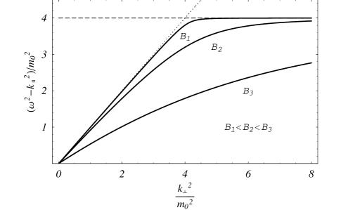
Figure 1: Dispersion curves for second mode in the first cyclotron resonance for different values of weak field. The dotted line represent the light cone curve, the dashed line correspond to the threshold energy for pair formation $k_{\perp}^{2}=4m_{0}^{2}$.

For values of energies and magnetic fields for which the exponential factor in (16) is of order unity we get

$$\omega^{2}=k_{\parallel}^{2}-\frac{kF^{2}k}{2\mathcal{F}}\left(1-\frac{2\mu^{\prime}B}{m_{0}}\right)$$

which we can be approximated as

$$\omega=|\textbf{k}|+\frac{\mu^{\prime}B}{m_{0}|\textbf{k}|}\frac{kF^{2}k}{2\mathcal{F}}$$

In such case the magnetic moment is determined by

$$\mu_{\gamma}=-\frac{\mu^{\prime}}{m_{0}|\textbf{k}|}\frac{kF^{2}k}{2\mathcal{F}}$$ (18)

in the case of perpendicular propagation

$$\mu_{\gamma}^{max}=\frac{\mu^{\prime}k_{\perp}}{m_{0}}$$ (19)

For perpendicular propagation to $B_{z}$, $(k_{\parallel}=0)$, and although the present approximation is not strictly valid for $k_{\perp}\to 2m_{0}$ the photon anomalous magnetic moment is of order

$$\mu_{\gamma}\sim 2\mu^{\prime}$$ (20)

Below we will get a larger value near the first pair creation threshold. In the table below we show some $\mu_{\gamma}^{max}$ values such that $\exp\left[-\frac{k_{\perp}^{2}}{2m_{0}}\frac{B_{c}}{B}\right]\sim 1$ corresponding to ranges of $X$- rays energies and magnetic field values.

	$\omega=m_{0}10^{-8}$	$B=1$ G	$\omega=m_{0}10^{-6}$	$B=10^{4}$ G	$\omega=m_{0}10^{-4}$	$B=10^{8}$ G	$\omega=m_{0}10^{-2}$	$B=10^{12}$ G
$\mu_{\gamma}^{max}$	$10^{-8}\mu^{\prime}$		$10^{-6}\mu^{\prime}$		$10^{-4}\mu^{\prime}$		$10^{-2}\mu^{\prime}$

According to (12) the refraction index in the weak field approximation and low frequency limit is given by

$$n^{(2)}=1+\frac{\mu^{\prime}k_{\perp}^{2}}{m_{0}|\textbf{k}|^{2}}B.$$

It must be noticed that when the propagation is perpendicular to $B_{z}$ the refraction index is maximum

$$n_{\perp}^{(2)}=1+\frac{\mu^{\prime}}{m_{0}}B$$

From (13) and (14) we obtain that the absolute value of the group velocity is given by

$$\textrm{v}^{(2)}\simeq 1-\frac{\mu_{\gamma}^{(2)}}{|\textbf{k}|}B.$$ (21)

in the last expression we neglected the term $B_{z}$ squared. In the particular case $k_{\parallel}=0$

$$\textrm{v}_{\perp}^{(2)}=1-\frac{\mu^{\prime}}{m_{0}}B.$$ (22)

In the asymptotic region of supercritical magnetic fields $B\gg B_{c}$ and restricted energy of longitudinal motionProceeding Shabad (1979) $\omega^{2}-k_{\parallel}^{2}\ll(B/B_{c})m_{0}^{2}$, in the low frequency limit the behavior of the photon propagating in the second mode is equal to the case of weak magnetic field (16). When the magnetic field $B\sim B_{c}$, the photon magnetic moment can be approximated by (18). For a typical $X$ ray photon of wavelength $\sim$ Å, and propagation perpendicular to $B_{z}$, its magnetic moment has values of order $\mu_{\gamma}\sim 10^{-2}\mu^{\prime}$ in this case. This behavior is also present in the photon-positronium mixed state.

IV The Cyclotron Resonance

Similarly to the case of strong magnetic field $(B\gtrsim B_{c})$, the singularity corresponding to cyclotron resonance appears in the second mode when $B\ll B_{c}$. The corresponding eigenvalue near of the first pair creation threshold is given by

$$\pi_{2}=\frac{2\alpha m_{0}^{3}B}{B_{c}}\exp\left(\frac{kF^{2}k}{4m_{0}^{2}\mathcal{F}}\frac{B_{c}}{B}\right)\left[4m_{0}^{2}+\left(k^{2}+\frac{kF^{2}k}{2\mathcal{F}}\right)\right]^{1/2},\\$$ (23)

The term $\exp(kF^{2}kB_{c}/4m_{0}^{2}\mathcal{F}B)$ plays an important role in the cyclotron resonance, both in the weak and the large field regime. The solution of the equation (4) for the second mode (first obtained by Shabad shabad (1975)) is shown schematically in Fig 1. In this picture, it is noted the departure of the dispersion law from the light cone curve. For the first threshold the deflection increases with increasing external magnetic field. In the vicinity of the first threshold the solutions of (4) and (23) are similar to the case of strong magnetic field regime, therefore, in order to show the results in a more compact form let us use the form used in Hugo and Shabad (1979). In it the eigenvalues of $\Pi_{\mu\nu}(k|A_{\mu}^{ext})$ near the thresholds can be written approximately as

$$\pi_{n,n^{\prime}}^{(i)}\approx-\frac{2\pi\phi_{n,n^{\prime}}^{(i)}}{|\Lambda|}$$ (24)

with $|\Lambda|=((k_{\perp}^{\prime 2}-k_{\perp}^{\prime\prime 2})(k_{\perp}^{\prime 2}+k^{2}+\frac{kF^{2}k}{\mathcal{F}}))^{1/2}$ and

$$k_{\perp}^{\prime\prime 2}=m_{0}^{2}\left[(1+2\frac{B}{B_{c}}n)^{1/2}-(1+2\frac{B}{B_{c}}n^{\prime})^{1/2}\right]^{2},$$ (25)

where $k_{\perp}^{\prime 2}$ is the squared threshold energy for $e^{\pm}$ pair production, and $k_{\perp}^{\prime\prime 2}$ is the squared threshold energy for excitation between Landau levels $n,n^{\prime}$ of an electron or positron. The functions $\phi_{n,n^{\prime}}^{(i)}$ are rewritten from Hugo and Shabad (1979) in the Appendix B.

In the vicinity of the first resonance $n=n^{\prime}=0$ and considering $k_{\perp}\neq 0$ and $k_{\parallel}\neq 0$, according to shabad (1972, 1975) the physical eigenwaves are described by the second and third modes, but only the second mode has a singular behavior near the threshold and the function $\phi^{(2)}_{nn^{\prime}}$ has the structure

$$\phi_{0,0}^{(2)}\simeq-\frac{2\alpha Bm_{0}^{4}}{\pi B_{c}}\textrm{exp}\left(\frac{kF^{2}k}{4m_{0}^{2}\mathcal{F}}\frac{B_{c}}{B}\right)$$ (26)

In this case $k_{\perp}^{\prime\prime 2}=0$ and $k_{\perp}^{\prime 2}=4m_{0}^{2}$ is the threshold energy.

When $\textbf{B}=\textbf{B}_{z}$, the scalar $kF^{2}k/2\mathcal{F}=-k_{\perp}^{2}$ and the approximation of the modes (24) turns the dispersion equation (50) into a cubic equation in the variable $z_{1}=\omega^{2}-k_{\parallel}^{2}$ that can be solved by applying the Cardano formula. We will refer in the following to (5) as the real solution of this equation.

We would define the function

$$\Lambda^{*}=(k_{\perp}^{\prime\prime 2}-k_{\perp}^{\prime 2})(k_{\perp}^{2}-k_{\perp}^{\prime 2})$$ (27)

to simplify the form of the solutions (5) of the equation (50). The functions $f_{i}$ are dependent on $k_{\perp}^{2},k_{\perp}^{\prime 2},k_{\perp}^{\prime\prime 2},B$, and are

$$f_{i}^{(1)}=\frac{1}{3}\left[2k_{\perp}^{2}+k_{\perp}^{\prime 2}+\frac{\Lambda^{*2}}{(k_{\perp}^{\prime\prime 2}-k_{\perp}^{\prime 2})\mathcal{G}^{1/3}}+\frac{\mathcal{G}^{1/3}}{k_{\perp}^{\prime\prime 2}-k_{\perp}^{\prime 2}}\right]$$ (28)

where

$$\mathcal{G}=6\pi\sqrt{3}D-\Lambda^{*3}+54\pi^{2}\phi_{n,n^{\prime}}^{(i)2}(k_{\perp}^{\prime\prime 2}-k_{\perp}^{\prime 2})^{2}$$

with

$$D=\sqrt{-(k_{\perp}^{\prime 2}-k_{\perp}^{\prime\prime 2})^{2}\Lambda^{*3}\phi_{n,n^{\prime}}^{(i)2}\left[1-\frac{27\pi^{2}\phi_{n,n^{\prime}}^{(i)2}(k_{\perp}^{\prime\prime 2}-k_{\perp}^{\prime 2})^{2}}{\Lambda^{*3}}\right]}$$

The solution $z_{1}=f_{i}^{(1)}$, where $z_{1}=\omega^{2}-k^{2}_{\parallel}$, concern the values of $k_{\perp}^{2}$ exceeding the root $k_{\perp}^{\ast 2}$ of the equation $D=0$, approximately equal to

$$k_{\perp}^{\star 2}\simeq k_{\perp}^{\prime 2}-3\left(\frac{\pi^{2}\phi_{n,n^{\prime}}^{(i)2}(k_{\perp}^{\prime 2})}{k_{\perp}^{\prime\prime 2}-k_{\perp}^{\prime 2}}\right)^{1/3}$$

(for $k_{\perp}^{2}<k_{\perp}^{*2}$, $D$ becomes complex). Besides (28), there are two other solutions of the above- mentioned cubic equation resulting from substituting (24) in (50). These are complex solutions and are located in the second sheet of the complex plane of the variable $z_{1}=\omega^{2}-k_{\parallel}^{2}$. At $k_{\perp}^{2}>k_{\perp}^{\ast 2}$ these two complex solutions are given by

$$f_{i}^{(2)}=\frac{1}{6}\left[2(2k_{\perp}^{2}+k_{\perp}^{\prime 2})-\frac{(1+i\sqrt{3})\Lambda^{*2}}{(k_{\perp}^{\prime\prime 2}-k_{\perp}^{\prime 2})\mathcal{G}^{1/3}}-\frac{(1-i\sqrt{3})\mathcal{G}^{1/3}}{k_{\perp}^{\prime\prime 2}-k_{\perp}^{\prime 2}}\right]$$

and

$$f_{i}^{(3)}=\frac{1}{6}\left[2(2k_{\perp}^{2}+k_{\perp}^{\prime 2})-\frac{(1-i\sqrt{3})\Lambda^{*2}}{(k_{\perp}^{\prime\prime 2}-k_{\perp}^{\prime 2})\mathcal{G}^{1/3}}-\frac{(1+i\sqrt{3})\mathcal{G}^{1/3}}{k_{\perp}^{\prime\prime 2}-k_{\perp}^{\prime 2}}\right]$$

but they are not interesting to us in the present context.

We should define the functions

$$m_{n}=\frac{k_{\perp}^{\prime}+k_{\perp}^{\prime\prime}}{2}\ \ \textrm{and}\ \ m_{n^{\prime}}=\frac{k_{\perp}^{\prime}-k_{\perp}^{\prime\prime}}{2},$$

which are positive for all possible values of $n$ and $n^{\prime}$.

Now the magnetic moment of the photon can be derived by taking the implicit derivative $\partial\omega/\partial B_{z}$ and $\partial\omega/\partial kF^{2}k$ in the dispersion equation, from (4) and (24) it is obtained that

$$\mu_{\gamma}^{(i)}=\frac{\pi}{2\omega(|\Lambda|^{3}-4\pi\phi_{n,n^{\prime}}^{(i)}m_{n}m_{n^{\prime}})}\left[\phi_{n,n^{\prime}}^{(i)}\left(A\frac{\partial m_{n}}{\partial B}+Q\frac{\partial m_{n^{\prime}}}{\partial B}\right)-2\Lambda^{2}\frac{\partial\phi_{n,n^{\prime}}^{(i)}}{\partial B}\right]$$ (29)

being

$$A=-4m_{n^{\prime}}[z_{1}-(m_{n}+m_{n^{\prime}})(3m_{n}+m_{n^{\prime}})]>0$$

and

$$Q=-4m_{n}[z_{1}-(m_{n}+m_{n^{\prime}})(m_{n}+3m_{n^{\prime}})]>0.$$

The expression (29) contains terms with paramagnetic and diamagnetic behavior, in which, as is typical in the relativistic case, the dependence of $\mu$ on $B$ is non-linear. It contains also diamagnetic terms, depending on the sign of $\phi_{n,n^{\prime}}^{(i)}$ and its derivatives with regard to $B$: if $\phi_{n,n^{\prime}}^{(i)}>0$ the first term in the bracket, contributes paramagnetically ($\frac{\partial m_{n}}{\partial B}\geq 0$ and $\frac{\partial m_{n^{\prime}}}{\partial B}\geq 0$), if $\phi_{n,n^{\prime}}^{(i)}<0$ the sign of this term is opposite and its contribution is diamagnetic. The second term of (29) will be paramagnetic or diamagnetic depending on the sign of the derivative of the $\phi_{n,n^{\prime}}^{(i)}$ with regard to $B$.

In particular if $n=n^{\prime}$

$$\mu_{\gamma}^{(i)}=\frac{\pi}{\omega(|\Lambda|^{3}-4\pi\phi_{n}^{(i)}m_{n}^{2})}\left[\phi_{n}^{(i)}A\frac{\partial m_{n}}{\partial B}-\Lambda^{2}\frac{\partial\phi_{n}^{(i)}}{\partial B}\right]$$ (30)

with $A=-4m_{n}[z_{1}-8m_{n}^{2}]>0$

In the vicinity of the first threshold $k_{\perp}^{\prime\prime 2}=0$, $k_{\perp}^{\prime 2}=4m_{0}^{2}$ and $\partial m_{n}/\partial B=0$ when $n=0$, therefore for the second mode the absolute value of the magnetic moment is given by

$$\mu_{\gamma}^{(2)}=-\frac{\pi|\Lambda|^{2}}{\omega\left(|\Lambda|^{3}-4m_{0}^{2}\pi\phi_{00}^{(2)}\right)}\frac{\partial\phi_{00}^{(2)}}{\partial B}$$ (31)

One can write the (31) in explicit form as

$$\mu_{\gamma}^{(2)}=\frac{\alpha m_{0}^{3}\left(4m_{0}^{2}+k^{2}+\frac{kF^{2}k}{2\mathcal{F}}\right)\exp\left(\frac{kF^{2}k}{4m_{0}^{2}\mathcal{F}}\frac{B_{c}}{B}\right)}{\omega B_{c}\left[(4m_{0}^{2}+k^{2}+\frac{kF^{2}k}{2\mathcal{F}})^{3/2}+\alpha m_{0}^{3}\frac{B}{B_{c}}\exp\left(\frac{kF^{2}k}{4m_{0}^{2}\mathcal{F}}\frac{B_{c}}{B}\right)\right]}\left(1-\frac{kF^{2}k}{4m_{0}^{2}\mathcal{F}}\frac{B_{c}}{B}\right).$$ (32)

if we consider for simplicity propagation perpendicular to the field $B$, and $\omega$ near the threshold $2m_{0}$, the function $\mu_{\gamma}^{(2)}=f(X)$, where $X=\sqrt{4m_{0}^{2}-\omega^{2}}$ has a maximum for $X={\pi\phi_{00}^{(2)}/m_{0}}^{1/3}$, which is very near the threshold.

Thus, for perpendicular propagation the expression (32) has a maximum value when $k_{\perp}^{2}\simeq k_{\perp}^{\prime 2}$. Therefore in a vicinity of the first pair creation threshold the magnetic moment of the photon has a paramagnetic behavior and a resonance peak whose value is given by

$$\mu_{\gamma}^{(2)}=\frac{m_{0}^{2}(B+2B_{c})}{3m_{\gamma}B^{2}}\left[2\alpha\frac{B}{B_{c}}\exp\left(-\frac{2B_{c}}{B}\right)\right]^{2/3}$$ (33)

We would like to define the ”dynamical mass” $m_{\gamma}$ of the photon in presence of a strong magnetic field by the equation

$$m_{\gamma}^{(2)}=\omega(k_{\perp}^{\prime 2})=\sqrt{4m_{0}^{2}-m_{0}^{2}\left[2\alpha\frac{B}{B_{c}}\exp\left(-\frac{2B_{c}}{B}\right)\right]^{2/3}}$$ (34)

From (33) it is seen that near the pair creation threshold, the magnetic moment induced by the external field in the photon as a result of its interaction with the polarized electron-positron quanta of vacuum, has a peak (Fig. 3). This is a resonance peak, and we understand it as due to the interaction of the photon with the polarized $e^{\pm}$ pairs.

The expression (33) presents a maximum when $B\simeq B_{c}$, in such case the magnetic moment is given by

$$\mu_{\gamma}^{(2)}\approx 3\mu^{\prime}\left(\frac{1}{2\alpha}\right)^{1/3}\approx 12.85\mu^{\prime}$$ (35)

The arising of a photon dynamical mass is a consequence of the radiative corrections, which become significant for photon energies near the pair creation threshold and magnetic fields large enough to make significant the exponential term $\exp(kF^{2}kB_{c}/4m_{0}^{2}\mathcal{F}B)=e^{-k_{\perp}^{2}/eB}$. This means that the massless photon coexists with the massive pair, leading to a behavior very similar to that of a neutral vector particle osipov (1979) bearing a magnetic moment.One should notice from (34) that the dynamical mass decrease with the increasing field intensity, which suggests that the interaction energy of the photon with its environment increase for magnetic fields far greater than $B_{c}$ near the first threshold, when the photon coexist with the virtual pair.

The problem of neutral vector particles is studied elsewhere Hugo Aurora y Herman (1979). The energy eigenvalues being

$$E(p,B,\eta)=\sqrt{p_{3}^{2}+p_{\perp}^{2}+M^{2}+\eta(\sqrt{p_{\perp}^{2}+M^{2}})qB},$$ (36)

where the second square root expresses the dependence of the eigenvalues on the ”transverse energy”, proportional to the scalar $pF^{2}p/{\cal F}$. We have $\eta=0,\pm 1$, and $q$ being a quantity having the dimensions of magnetic moment. In what follows we exclude the value $\eta=0$, since it corresponds to the case of no interaction with the external field $B$. We have that for $\eta=-1$ the magnetic moment is $\mu=\pm\frac{q}{\sqrt{M^{2}-MqB}}$, which is divergent at the threshold $M=qB$. The behavior of the photon near the critical field $B_{c}$ closely resembles this behavior, since it has a maximum value at the threshold.

For $B_{z}\gg B_{c}$ although the vacuum is strongly polarized, the photon shows a weaker polarization, i.e the contribution from the singular behavior near the thresholds decreases. Actually, the propagation is being decreased due to an increasing in the imaginary part of the photon energy $\Gamma$ (we have the total frequency $\omega=\omega_{r}+i\Gamma$, where $\omega_{r}$ is the real part of it). As the modes are bent to propagate parallel to $B$, they propagate in an increasingly absorbent medium. But for $B>>B_{c}$ we are in a region beyond QED and new phenomena related to the standard model may appear, as for instance, the creation of $\mu^{\pm}$ pairs, and their subsequent decay according to the allowed channels.

As opposite to the second mode case, the polarization eigenvalue from the third mode in supercritical magnetic field does not manifest a singular behavior in the first resonance Proceeding Shabad (1979). In this case the eigenvalues are given by

$$\pi_{3}=\frac{\alpha k^{2}}{3\pi}\left(\ln\frac{B}{B_{c}}-C\right)+\frac{\alpha}{3\pi}\left(0.21\frac{kF^{2}k}{2\mathcal{F}}-1.21\left(k^{2}+\frac{kF^{2}k}{2\mathcal{F}}\right)\right)$$ (37)

In this case the dispersion equation has the solution

$$\omega^{2}=|\textbf{k}|^{2}+\frac{kF^{2}k}{2\mathcal{F}}\left[1-\frac{\alpha}{3\pi}\left(\ln\frac{B}{B_{c}}-C-1.21\right)\right]^{-1}$$ (38)

being $C$ is Euler constant. For fields $B\sim B_{c}$ so that the logarithmic terms are small, the corresponding magnetic moment is given by

$$\mu_{\gamma}^{(3)}=\frac{2\mu^{\prime}}{3m_{0}}\frac{k_{\perp}^{2}}{\omega}$$ (39)

for perpendicular propagation to $B_{z}$ and for photons with energies near of $m_{0}$ the magnetic moment of the photon propagating in the third mode has a value of $\mu_{\gamma}^{(3)}\sim\mu^{\prime}$.

V Magnetic Moment For The Photon-Positronium Mixed States

In the case of positronium formation, by following shabad (1983); Leinson (1979), neglecting the retardation effect and in the lowest adiabatic approximation, the Bethe-Salpeter equation is reduced to a Schrödinger equation in the variable $(z^{e}-z^{p})$ which governs the relative motion along B of the electron and positron.

Under such approximations, the conservation law induced by the traslational invariance takes the form $p_{x}=p_{x}^{p}+p_{x}^{e}=k_{\perp}$. Therefore the binding energy depends on the distance between the $y$-coordinates of the centers of the electron and positron orbits $|y_{0}^{p}-y_{0}^{e}|=p_{x}/\sqrt{eB}$.

The Schrödinger equation mentioned includes the attractive coulomb force whose potential in our case has the form

$$V_{nn^{\prime}}(z^{e}-z^{p})=-\frac{e^{2}}{\sqrt{(z^{e}-z^{p})^{2}+L^{4}p_{x}^{2}}}$$

where $L=(eB)^{-1/2}$ is the radius of the electron orbit. The eigenvalue of this equation $\Delta\varepsilon_{n,n^{\prime}}(n_{c},k_{\perp}^{2})$ is the binding energy of the particles which is numbered by a discrete number $n_{c}$ that identifies the Coulomb-bound state for $\Delta\varepsilon_{n,n^{\prime}}(n_{c},k_{\perp}^{2})>0$ and by a continuous one in the opposite case.

The energy of the pair which does not move along the external magnetic field is given by

$$\varepsilon_{n,n^{\prime}}(n_{c},k_{\perp}^{2})=k_{\perp}^{\prime}+\Delta\varepsilon_{n,n^{\prime}}(n_{c},k_{\perp}^{2})$$ (40)

In this paper we will consider the case in which the Coulomb state is $n_{c}=0$, here the binding energy is given by the expression of the eigenvalues of this equation,

$$\Delta\varepsilon_{n,n^{\prime}}(0,k_{\perp}^{2})=-\frac{\alpha^{2}M_{r}}{2}\left(2\ln\left[\frac{a_{nn^{\prime}}^{B}}{2\sqrt{L^{2}+L^{4}P_{x}^{2}}}\right]\right)^{-2},$$ (41)

where $a_{B}^{nn^{\prime}}=1/e^{2}M_{r}$ is Bohr radius and $M_{r}=m_{n}m_{n^{\prime}}/(m_{n}+m_{n^{\prime}})$ the reduced mass of the bound pair.

The dispersion equation of the positronium is given by

$$k_{\perp}^{2}+k_{\parallel}^{2}-\omega^{2}=-\frac{2\pi\Phi_{nn^{\prime}n_{c}}^{(i)}}{\varepsilon_{nn^{\prime}}^{2}-\omega^{2}+k_{\parallel}^{2}}$$ (42)

For each set of discrete quantum number $n$, $n^{\prime}$, $n_{c}$, equation (42) is quadratic with regard to the variable $z_{1}=\omega^{2}-k_{\parallel}^{2}$ and its solutions are

$$f_{i}=\frac{1}{2}\left(\varepsilon_{nn^{\prime}n_{c}}^{2}(k_{\perp}^{2})+[k_{\perp}^{2}\pm\right.$$ (43)

$$\left.(\varepsilon_{nn^{\prime}n_{c}}^{2}(k_{\perp}^{2})-k_{\perp}^{2})^{2}-8\pi\Phi_{nn^{\prime}n_{c}}^{(i)}(k_{\perp}^{2})]^{1/2}\right)$$

At the first cyclotron resonance $n=n^{\prime}=0$, the function $\Phi_{000}$ that define the second mode has the structure

$$\Phi_{000}^{(2)}=\phi_{00}^{(2)}\varepsilon_{000}(k_{\perp}^{2})|\psi_{000}(0)|^{2}$$ (44)

with

$$\Delta\varepsilon_{00}(0,k_{\perp}^{2})=-\alpha^{2}m_{0}\left(\ln\left[\frac{1}{\alpha}\sqrt{\frac{B_{c}(1+\frac{k_{\perp}^{2}B_{c}}{m_{0}^{2}B})}{B}}\right]\right)^{2}$$

where

$$|\psi_{000}(0)|^{2}=\alpha\left|\ln\left[\frac{1}{\alpha}\sqrt{\frac{B}{B_{c}\left(1+\frac{k_{\perp}^{2}B_{c}}{m_{0}^{2}B}\right)}}\right]\right|$$

is the wave function squared of the longitudinal motionLoundon (1979) at $z^{e}=z^{p}$.

In the case of photon-positronium mixed states we obtain from (7) and (42) that

$$\mu_{\gamma}^{P}=\frac{\pi\Upsilon}{\omega(k_{\parallel}^{2}-\omega^{2}-\varepsilon^{2})\left(1+\frac{2\pi\Phi_{nn^{\prime}n_{c}}^{(i)}}{k_{\parallel}^{2}-\omega^{2}-\varepsilon^{2}}\right)}$$ (45)

being

$$\Upsilon=\varepsilon_{nn^{\prime}}(n_{c})\Phi_{nn^{\prime}n_{c}}^{(i)}\frac{\partial\varepsilon}{\partial B}-\frac{\partial\Phi_{nn^{\prime}n_{c}}^{(i)}}{\partial B}$$

Following the reasoning of (33), for magnetic fields $B\gg B_{c}$ one can define the dynamical mass of the photon-positronium mixed state in the first threshold for positronium energy, $\varepsilon^{2}\sim 3.996m_{0}^{2}$ and perpendicular propagation as

$$m_{\gamma}^{P}=\sqrt{\varepsilon_{00}^{2}-2m_{0}^{2}\alpha\left[\frac{B}{B_{c}}\ln\left(\frac{1}{2\alpha}\frac{B}{B_{c}}\right)\right]^{1/2}}$$ (46)

in this regime

$$\mu_{\gamma}^{P}=\frac{m_{0}^{2}\alpha\left(1+\ln\left[\frac{B}{2\alpha B_{c}}\right]\right)}{2B_{c}m_{\gamma}^{P}\sqrt{\frac{B}{B_{c}}\ln\left[\frac{B}{2\alpha B_{c}}\right]}}$$ (47)

when $k_{\parallel}=0$.

In a similar way to the free pair creation, the behavior of the magnetic moment of the magnetic moment of the mixed state for $n,n^{\prime}\neq 0$ can be paramagnetic for some values of Landau numbers and intervals in momentum space, and diamagnetic in other ones.

VI Results and discussion

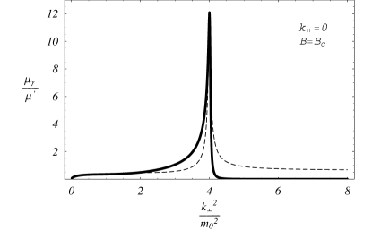
For perpendicular propagation the dependence of the magnetic moment with regard $k_{\perp}^{2}$ in the first resonance $k_{\perp}^{\prime 2}=4m_{0}^{2}$ is displayed in FIG. 2 for free pair creation and photon-positronium mixed state. Both curves show the same qualitative behavior. As it was expected, near the threshold energy appears the peak characteristic of the resonance. The result shows that near the pair creation threshold the magnetic moment of a photon may have values greater than the anomalous magnetic moment of the electron. (Numerical calculations range from 0 to more than $12\mu^{\prime}$). This result is related to the probability of the pair creation, which is maximum in the first resonant form when $k_{\perp}=2m_{0}$, and increase with $B$, because the medium is becoming absorbent.

Figure 2: Magnetic moment curves of the photon (dark) and photon-positronium mixed states (dashed) with regard to perpendicular momentum squared, for the second mode $k_{\perp}^{\prime 2}=4m_{0}^{2}$ with $n=n^{\prime}=0$.

We observe that near the thresholds the behavior of the curves is the same for all pairs $\omega$, $k_{\parallel}$ satisfying the condition $\omega^{2}-k_{\parallel}^{2}=k_{\perp}^{\prime 2}$.

In all curves the magnetic moment decrease for momentum values $k_{\perp}^{2}>4m_{0}^{2}$. Therefore the vacuum polarization decreases, thus, the magnetic moment tends to vanish as it is shown in FIG. 2. We interpret these results in the sense that for photons with squared transversal component of the momenta greater than $4m_{0}^{2}$ the probability of free pair creation in the Landau ground state (and positronium creation) decrease very fast, since that region of momenta is to be considered inside the transparency region corresponding to the next thresholds, i.e., $n=0,n^{\prime}=1$ or vice-versa.

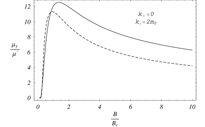
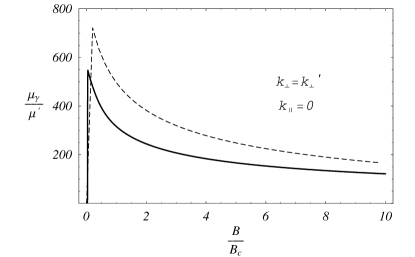
Figure 3: Magnetic moment curves for the photon and photon-positronium mixed states with regard to external magnetic field strength. The propagation is perpendicular to B and the values of the perpendicular momentum are equal to the absolute values of the free and bound threshold energies. The first (continuous) curve refers to the photon whereas the second (dashed) corresponds to the photon-positronium mixed state.

The behavior of the magnetic moment with regard to the field is shown in the FIG. 3 for the case of photon and photon-positronium mixed state. The picture was obtained in the field interval $0\leq B\leq 10B_{c}$ by considering perpendicular propagation and taking the values of the momentum squared as equal to the absolute values of the threshold energies of free and bound pair creation. Here, as opposite to the case of low frequency, the magnetic moment of the photon tend to vanish when $B\rightarrow 0$. We note that, again, the magnetic moment of the photon is greater than $\mu^{\prime}$. In correspondence with figs. 2 the magnetic moment of the photon not considering Coulomb interaction, is greater than the corresponding to photon-positronium mixed state. This result is to be expected due to the existence of the binding energy, in the latter case it entails a decrease of the threshold energy. Each curve has a maximum value, this maximum for the free pair creation is approximately $B\approx 1.5B_{c}$, whereas for photon-positron bound state the value is $B\approx B_{c}$.

Figure 4: Photon dynamical mass dependence with regard the external magnetic field of the photon-positronium (dashed) and photon-free pair (dark) mixed states. Both curves were obtained near the corresponding first thresholds for each process.

In fig. 4 we display the photon dynamical mass dependence on the magnetic field, by considering perpendicular propagation near the thresholds, for free and bound pair creation and for the second mode. It is shown that for that mode, the dynamical mass decreases with increasing magnetic field.

For magnetic field values $B>1.5B_{c}$ the dynamical mass of the photon-positronium mixed state is greater than the corresponding to the case of free pair creation which suggests that the latter is more probable that the bound state case.

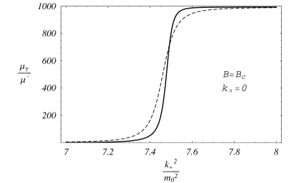
Figure 5: Curves for the modulus of the photon magnetic moment with regard to the perpendicular momentum squared, near the pair creation threshold for the second mode $k_{\perp}^{\prime 2}=7.46m_{0}^{2}$ with $n=0$, $n^{\prime}=1$ and for perpendicular propagation. The value of the external magnetic field used for calculation are $B=B_{c}$. The dashed line correspond to photon-positronium mixed state, whereas the dark line to the free pair creation.

We have found that when the particles are created in excited states the behavior of the magnetic moment reaches higher values with regard the case analyzed previously when $k_{\perp}^{2}=k_{\perp}^{\prime 2}$ and $B\backsim B_{c}$. Calculation points out that these values may be of order $10^{2}\mu^{\prime}$. The new values obtained come fundamentally due to the fact of the threshold energies, which depend on the magnetic field B (see Fig.2). The new behavior of the photon and photon-positronium mixed state is shown in the Fig.5 and Fig. 6.

Figure 6: Curves for the modulus of the photon magnetic moment (dark) and photon-positronium mixed states(dashed) plotted with regard to the external magnetic field strength when the propagation is perpendicular to B and the values of the perpendicular momentum squared is equal to the values of the free and bound threshold energies for $n=0$ and $n^{\prime}=1$.

In this case the dynamical mass Fig.7, as different from the previous case, increases with increasing magnetic field. This means that the magnetic field confine the virtual particles near the threshold when these tend to be created in excited states. The dynamical mass of the positronium in such conditions is always smaller than the corresponding to free pair creation, which suggests that the bound state pair creation in this configuration is more probable.

Figure 7: Photon dynamical mass dependence with regard the external magnetic field of the photon-positronium (dashed) and photon-free pair (dark) being $n=0$ and $n^{\prime}=1$. Both curves were obtained in the corresponding energy thresholds.

VII Conclusion

We conclude, first, that a photon propagating in vacuum in presence of an external magnetic field, exhibits a nonzero magnetic moment and a sort of dynamical mass due to the magnetic field. This phenomenon occurs whenever the photon has a nonzero perpendicular momentum component to the external magnetic field. The values of this anomalous magnetic moment depend on the propagation mode and magnetic field regime. The maximum value taken by the photon magnetic moment is greater than the anomalous magnetic moment of the electron in a strong magnetic field.

Second, in the small field and low frequency approximations, the magnetic moment of the photon also exists and is slowly dependent of the magnetic field intensity in some range of frequencies, whereas the high frequency limit it depends on $|\bf{B}|$. In both cases it vanishes when $B\to 0.$

Under these conditions, the behavior of the photon is similar to a vector neutral massive particle.

VIII Acknowledgement

Both authors are greatly indebted to Professor A.E. Shabad, from P. N.Lebedev Physical Institute in Moscow for several comments and illuminating discussions.

IX Appendix A

The three eigenvalues $\pi_{i}=1,2,3$ of the polarization operator in one loop approximation, calculated using the exact propagator of electron in an external magnetic field, can be expressed as linear combination of three functions $\Sigma_{i}$. In what follows we will call $x=B/B_{c}$

$$\pi_{1} =-\frac{1}{2}k^{2}\Sigma_{1},$$ (48)

$$\pi_{2} =-\frac{1}{2}\left(\left(\frac{kF^{2}k}{2\mathcal{F}}+k^{2}\right)\Sigma_{2}-\frac{kF^{2}k}{2\mathcal{F}}\Sigma_{1}\right),$$ (49)

$$\pi_{3} =-\frac{1}{2}\left(\left(\frac{kF^{2}k}{2\mathcal{F}}+k^{2}\right)\Sigma_{1}-\frac{kF^{2}k}{2\mathcal{F}}\Sigma_{3}\right).$$ (50)

where $\mathcal{F}=\frac{B^{2}}{2}$ and

We express

$$\Sigma_{i}=\Sigma_{i}^{(1)}+\Sigma_{i}^{(2)},$$ (51)

being

$$\Sigma_{i}^{(1)}(x)=\frac{2\alpha}{\pi}\int_{0}^{\infty}dte^{-t/x}\int_{-1}^{1}d\eta\left[\frac{\sigma_{i}(t,\eta)}{\sinh t}-\lim_{t\rightarrow 0}\frac{\sigma_{i}(t,\eta)}{\sinh t}\right]$$ (52)

and

$$\Sigma_{i}^{(2)}(x,kF^{2}k,k^{2},\mathcal{F})=\frac{2\alpha}{\pi}\int_{0}^{\infty}dte^{-t/x}\int_{-1}^{1}d\eta\frac{\sigma_{i}(t,\eta)}{\sinh t}\left[\exp\left(\frac{kF^{2}k}{2\mathcal{F}}\frac{M(t,\eta)}{m_{0}^{2}x}-\left(\frac{kF^{2}k}{2\mathcal{F}}+k^{2}\right)\frac{1-\eta^{2}}{4m_{0}^{2}x}t\right)-1\right],$$ (53)

where

$$M(t,\eta)=\frac{\cosh t-\cosh\eta t}{2\sinh t},$$ (54)

$$\sigma_{1}(t,\eta)=\frac{1-\eta}{2}\frac{\sinh(1+\eta)t}{\sinh t},$$ (55)

$$\sigma_{2}(t,\eta)=\frac{1-\eta^{2}}{2}\cosh t,$$ (56)

$$\sigma_{3}(t,\eta)=\frac{\cosh t-\cosh\eta t}{2\sinh^{2}t}.$$ (57)

Express $\Sigma_{i}^{(1)}$ as

$$\Sigma_{i}^{(1)}(x)=\frac{2\alpha}{\pi}\int_{0}^{\infty}dte^{-t/x}\left[\frac{g_{i}(t)}{\sinh t}-\frac{1)}{3t}\right].$$ (58)

Here

$$g_{i}(t)=\int_{-1}^{1}d\eta\sigma_{i}(t,\eta)d\eta$$

and in explicit form

$$g_{1}(t) =\frac{1}{4t\sinh t}\left(\frac{\sinh 2t}{t}-2\right),$$ (59)

$$g_{2}(t) =\frac{\cosh t}{3},$$ (60)

$$g_{3}(t) =\frac{1}{\sinh^{2}t}\left(\cosh t-\frac{\sinh t}{t}\right).$$ (61)

Let

$$u_{i}(t)=\frac{g_{i}(t)}{\sinh t}-\frac{1}{3t}$$ (62)

The asymptotic expansion of (62) in powers of $\exp(-t)$ have the form

$$u_{1}(t)=0,\ \ u_{2}(t)=1/3,\ \ u_{3}(t)=0$$ (63)

Our next purpose is to analyze the behavior of $\pi_{i}$ when $x\rightarrow 0$. In this case the behavior of $\Sigma_{i}^{(1)}(x)$ is determined by the the factor $\exp(-t/x)$ at the integrand which tends to zero when $x\rightarrow 0$. Taking in account the expansion

$$\exp(-t/x)\simeq\exp(-t/\epsilon)+\frac{\exp(-t/\epsilon)t}{\epsilon^{2}}(x-\epsilon),$$

integrating by $t$ and taking the limit when $\epsilon\rightarrow 0$ we obtain that

$$\Sigma_{1}^{(1)} (x)=0,\ \ \Sigma_{2}^{(1)}(x)\simeq\frac{2\alpha B}{3\pi B_{c}},\ \ \Sigma_{3}^{(1)}(x)=0.$$ (64)

The functions $\Sigma_{i}^{(2)}$ depend of three arguments, as indicated in (53). The asymptotic expansion of (55),(56), (57) in powers of $\exp(-t)$ and $\exp(t\eta)$ produces an expansion of (53) into a sum of contributions coming from the thresholds, the singular behavior in the threshold points originating from the divergencies of the $t-$integration in (53) near $t=\infty$ as it was made in shabad (1972). The leading term in the expansion of (55), (56), (57) at $t\rightarrow\infty$ are

$$\left.\left(\frac{\sigma_{1}(t,\eta)}{\sinh t}\right)\right|_{t\rightarrow\infty} =\frac{1-\eta}{2}\exp\left(-t(1-\eta)\right),$$ (65)

$$\left.\left(\frac{\sigma_{2}(t,\eta)}{\sinh t}\right)\right|_{t\rightarrow\infty} =\frac{1-\eta^{2}}{4},$$ (66)

$$\left.\left(\frac{\sigma_{3}(t,\eta)}{\sinh t}\right)\right|_{t\rightarrow\infty} =2\exp\left(-2t)\right).$$ (67)

The function $M(\infty,\eta)=1/2$, one obtains near the lowest singular threshold ($n=0$, $n^{\prime}=1$ or viceversa for $i=1$, $n=n^{\prime}=1$ for $i=1$, and $n=n^{\prime}=0$ for $i=2$). Taking into account this expansion we can write the expression (53) for the first and their modes as

$$\Sigma_{1}^{(2)}=\frac{4\alpha eB}{\pi}\int_{-1}^{1}d\eta(1-\eta)\left[\frac{\exp\left(\frac{kF^{2}k}{4m_{0}^{2}\mathcal{F}}\frac{B_{c}}{B}\right)}{4m_{0}^{2}+4(1-\eta)eB+\left(k^{2}+\frac{kF^{2}k}{2\mathcal{F}}\right)\left(1-\eta^{2}\right)}-\frac{1}{4m_{0}^{2}+4(1-\eta)eB}\right],$$ (68)

$$\Sigma_{2}^{(2)}=\frac{2\alpha eB}{\pi}\int_{-1}^{1}d\eta(1-\eta^{2})\exp\left(\frac{kF^{2}k}{4m_{0}^{2}\mathcal{F}}\frac{B_{c}}{B}\right)\left(\frac{1}{4m_{0}^{2}+\left(k^{2}+\frac{kF^{2}k}{2\mathcal{F}}\right)\left(1-\eta^{2}\right)}\right)-\frac{2\alpha eB}{3\pi m_{0}^{2}},$$ (69)

$$\Sigma_{3}^{(2)}=\frac{16\alpha eB}{\pi}\int_{-1}^{1}d\eta\exp\left(\frac{kF^{2}k}{4m_{0}^{2}\mathcal{F}}\frac{B_{c}}{B}\right)\left[\frac{1}{4m_{0}^{2}+8eB+\left(k^{2}+\frac{kF^{2}k}{2\mathcal{F}}\right)\left(1-\eta^{2}\right)}-\frac{1}{4m_{0}^{2}+8eB}\right].$$ (70)

In limit $x\to 0$ we get only one expression with singularity in the first threshold

$$\Sigma_{2}^{(2)}=\frac{2\alpha B}{3\pi B_{c}}\left(3m_{0}^{2}\int_{0}^{1}d\eta(1-\eta^{2})\frac{\exp\left(\frac{kF^{2}k}{4m_{0}^{2}\mathcal{F}}\frac{B_{c}}{B}\right)}{4m_{0}^{2}+\left(k^{2}+\frac{kF^{2}k}{2\mathcal{F}}\right)\left(1-\eta^{2}\right)}-1\right).$$ (71)

By carrying out the integration on $\eta$ we obtain

$$\Sigma_{2}^{(2)}=\frac{2\alpha B}{3\pi B_{c}}\left(3m_{0}^{2}\exp\left(\frac{kF^{2}k}{4m_{0}^{2}\mathcal{F}}\frac{B_{c}}{B}\right)\left[\frac{2}{k^{2}+\frac{kF^{2}k}{2\mathcal{F}}}-\frac{8m_{0}^{2}\arctan\left(\frac{k^{2}+\frac{kF^{2}k}{2\mathcal{F}}}{4m_{0}^{2}+k^{2}+\frac{kF^{2}k}{2\mathcal{F}}}\right)^{1/2}}{\left(4m_{0}^{2}+k^{2}+\frac{kF^{2}k}{2\mathcal{F}}\right)^{1/2}\left(k^{2}+\frac{kF^{2}k}{2\mathcal{F}}\right)^{3/2}}\right]-1\right).$$ (72)

Its behavior in the low frequency limit is given by

$$\Sigma_{2}^{(2)}=\frac{2\alpha B}{3\pi B_{c}}\left(3m_{0}^{2}\exp\left(\frac{kF^{2}k}{4m_{0}^{2}\mathcal{F}}\frac{B_{c}}{B}\right)\left[\frac{2}{k^{2}+\frac{kF^{2}k}{2\mathcal{F}}}-\frac{8m_{0}^{2}}{\left(4m_{0}^{2}+k^{2}+\frac{kF^{2}k}{2\mathcal{F}}\right)\left(k^{2}+\frac{kF^{2}k}{2\mathcal{F}}\right)}\right]-1\right),$$ (73)

which we can express as

$$\Sigma_{2}^{(2)}=\frac{2\alpha B}{3\pi B_{c}}\left(\frac{3m_{0}^{2}}{k^{2}+\frac{kF^{2}k}{2\mathcal{F}}}\exp\left(\frac{kF^{2}k}{4m_{0}^{2}\mathcal{F}}\frac{B_{c}}{B}\right)\left[2-\frac{8m_{0}^{2}}{\left(4m_{0}^{2}+k^{2}+\frac{kF^{2}k}{2\mathcal{F}}\right)}\right]-1\right)$$ (74)

therefore

$$\Sigma_{2}^{(2)}=\frac{2\alpha B}{3\pi B_{c}}\left(\frac{3}{2}\exp\left(\frac{kF^{2}k}{4m_{0}^{2}\mathcal{F}}\frac{B_{c}}{B}\right)-1\right).$$ (75)

Under such condition, by substituting the last one and the second expression of (64) in (50), we have that the second eigenvalue of the polarization operator can be written as

$$\pi_{2}=-\frac{2\mu^{\prime}B}{m_{0}}\left(\frac{kF^{2}k}{2\mathcal{F}}+k^{2}\right)\exp\left(\frac{kF^{2}k}{4m_{0}^{2}\mathcal{F}}\frac{B_{c}}{B}\right).$$ (76)

In the same approximation $\frac{kF^{2}k}{2\mathcal{F}}+k^{2}\approx\frac{kF^{2}k}{2\mathcal{F}}$ and

$$\pi_{2}=-\frac{2\mu^{\prime}B}{m_{0}}\frac{kF^{2}k}{2\mathcal{F}}\exp\left(\frac{kF^{2}k}{4m_{0}^{2}\mathcal{F}}\frac{B_{c}}{B}\right).$$ (77)

Now, the behavior $\pi_{2}$ near of the first threshold can be determined from (72) by taking into account the point $\omega^{2}-k_{\parallel}=4m_{0}^{2}-\epsilon$ with $\epsilon>0$ and $\epsilon\rightarrow 0$

$$\pi_{2}=\frac{2\alpha m_{0}^{3}B}{B_{c}}\exp\left(\frac{kF^{2}k}{4m_{0}^{2}\mathcal{F}}\frac{B_{c}}{B}\right)\left[4m_{0}^{2}+\left(k^{2}+\frac{kF^{2}k}{2\mathcal{F}}\right)\right]^{1/2}.$$ (78)

X Appendix B

The function $\phi_{n,n^{\prime}}^{(i)}$ is given by

$$\phi_{n,n^{\prime}}^{(1)}=-\frac{e^{2}}{4\pi^{2}}\frac{eBk^{2}}{z_{1}}\left[(2eB(n+n^{\prime})+z_{1})F_{n,n^{\prime}}^{(2)}-4k_{\perp}^{2}N_{n,n^{\prime}}^{(1)}\right],$$ (79)

$$\phi_{n,n^{\prime}}^{(2)}=-\frac{e^{2}}{4\pi^{2}}eB\left[\left(\frac{2e^{2}B^{2}(n-n^{\prime})^{2}}{z_{1}}+2m^{2}+eB(n+n^{\prime})\right)F_{n,n^{\prime}}^{(1)}+2eB(nn^{\prime})^{1/2}G_{n,n^{\prime}}^{(1)}\right],$$ (80)

$$\phi_{n,n^{\prime}}^{(3)}=-\frac{e^{2}}{4\pi^{2}}\frac{eBk^{2}}{z_{1}}\left[(2eB(n+n^{\prime})+z_{1})F_{n,n^{\prime}}^{(2)}+4k_{\perp}^{2}N_{n,n^{\prime}}^{(1)}\right],$$ (81)

where, calling $y=\frac{kF^{2}k}{4m_{0}^{2}\mathcal{F}}\frac{B_{c}}{B}$ and $z_{1}=k^{2}+\frac{kF^{2}k}{2\mathcal{F}}$

$$F_{n,n^{\prime}}^{(1)}=\left\{[L_{n^{\prime}-1}^{n-n^{\prime}}(y)]^{2}+\frac{n^{\prime}}{n}[L_{n^{\prime}}^{n-n^{\prime}}(y)]^{2}\right\}\frac{(n^{\prime}-1)!}{(n-1)!}y^{n-n^{\prime}}\exp[-y],$$

$$F_{n,n^{\prime}}^{(2,3)}=\left\{\frac{y}{n}[L_{n^{\prime}-1}^{n-n^{\prime}+1}(y)]^{2}\pm\frac{n^{\prime}}{x}[L_{n^{\prime}}^{n-n^{\prime}-1}(y)]^{2}\right\}\frac{(n^{\prime}-1)!}{(n-1)!}y^{n-n^{\prime}}\exp[-y],$$

$$G_{n,n^{\prime}}^{(1)}=2\left(\frac{n^{\prime}}{n}\right)^{1/2}\frac{(n^{\prime}-1)!}{(n-1)!}y^{n-n^{\prime}}L_{n^{\prime}-1}^{n-n^{\prime}}(y)L_{n^{\prime}}^{n-n^{\prime}}(y)\exp[-y],$$

$$N_{n,n^{\prime}}^{(1)}=\frac{n^{\prime}!}{(n-1)!}y^{n-n^{\prime}-1}L_{n^{\prime}-1}^{n-n^{\prime}+1}(y)L_{n}^{n-n^{\prime}-1}(y)\exp[-y].$$

Here $L_{n}^{m}(y)$ are generalized Laguerre polynomials. Laguerre polynomials with $-1$ for lower index must be taken as zero.

References

• shabad (1972) A. E. Shabad, Letter al Nuovo Cimento 2, 457 (1972).
• shabad (1975) A. E. Shabad, Ann. Phys. 90, 166 (1975).
• Usov and Shabad (1986) A. E. Shabad and V. V. Usov, Astrophys. space Sci. 128, 377 (1986).
• Usov and Shabad (1985) A. E. Shabad and V. V. Usov, Astrophys. space Sci. 102, 309 (1984).
• Proceeding Shabad (1979) A. E. Shabad, Procceding of the International Workshop on Strong Magnetic Field and Neutron Stars.Instituto de Cibernética Matemática y Física (ICIMAF, Havana) edited jointly by CBPF, Rio de Janeiro, ICIMAF, UFRGS, Porto Alegre, Brazil, 201, 2003.
• adler (1983) S. L. Adler, Phys. Rev. Lett. 77, 1695 (1996).
• adler (2002) V. V. Usov, ApJ L87, 572 (2002).
• Proceeding Elizabeth (1979) H. Pérez Rojas and E. Rodríguez Querts, Procceding of the International Workshop on Strong Magnetic Field and Neutron Stars.Instituto de Cibernética Matemática y Física (ICIMAF), 189, 2003.
• Heisenberg (1972) W. Heisenberg and H.  Euler, Z. Phys. 98, 714 (1936).
• schwinger (1951) J. Schwinger, Phys. Rev. 82, 664 (1951).
• Hugo and Shabad (1979) H. Pérez Rojas and A. E. Shabad, Ann. Phys. 121, 432 (1979).
• felipe aurora and shabad (1979) R. Gonzalez Felipe, A. Pérez Martinez and A. E. Shabad, Phys. Rev. A 43, 5575 (1991).
• Leinson (1979) L. B. Leinson and A. Pérez, JHEP 11, 039 (2000).
• shabad (1983) A. E. Shabad, Astrophys. Space Sci. 102, 327 (1983).
• Denisov and denisova (1986) V. I. Denisov, I. P. Denisova, and S. I. Svertilov, Doklady Akademii Nauk 380, 325 (2001).
• harding and baring (1986) M. G. Baring, and A. K. Harding, Astrophys. Space Sci. 547, 929 (2000).
• batalin (1971) I. A. Batalin and A. E. Shabad, JETP 33, 483 (1971).
• johson and lippman (1979) M. H Johnson and B. A. Lippmann, Phys. Rev. 76, 828 (1949).
• Hugo and Shabad (1979) H. Pérez Rojas and A. E. Shabad, Ann. Phys. 138, 1 (1982).
• osipov (1979) A. V. Kuznetsov, N. V. Mikheev, and M. V. Osipov Mod. Phys. Lett. A 17, 231 (2002).
• Hugo Aurora y Herman (1979) H. Pérez Rojas, A. Pérez Martínez, and H. J. Mosquera Cuesta Bose-Einstein condensates of neutral particles with non-zero magnetic moment placed in strong magnetic fields, to be published
• Loundon (1979) R. Loudon, Am. J. Phys. 27, 649 (1959).