Abstract

We present details of the analytic computation of the spectrum of lowest spin glueballs in pure Yang-Mills theory in 2+1 dimensions. The new ingredient is provided by the conjectured new non-trivial expression for the (quasi)Gaussian part of the ground state wave-functional. We show that this wave-functional can be derived by solving the Schrödinger equation under certain assumptions. The mass spectrum of the theory is determined by the zeros of Bessel functions, and the agreement with available lattice data is excellent.

1 Introduction and Summary

The understanding of the non-perturbative dynamics of pure Yang-Mills theory is one of the outstanding problems of theoretical physics. As was realised a long time ago, one of the persistent difficulties hampering any progress is the fact that we are studying a gauge theory, and it is clear that the fields that we use to define the theory (in the UV) do not create physical states, and are thus not the “correct degrees of freedom”. Instead one should switch to some set of gauge invariant variables. Traditionally, this has meant the Wilson loop operators, and the consequent introduction of the loop space formalism [2, 3, 4]. Although in some heuristic sense, this would seem to bear some relation to the expected appearance of a string theory, it is extremely difficult to proceed beyond a few basic stages. We believe that although the Wilson loop plays a central role in the theory, as its expectation value is a useful order parameter for confinement, it should not be thought of as representing the “correct degrees of freedom”.

Instead, building on a construction of Karabali, Kim and Nair [5], we suggest that the theory may be discussed in terms of local gauge invariant variables. The idea of reformulating Yang-Mills theory in terms of local gauge invariant variables is certainly not new and many such proposals exist in the literature [6, 7]. The unique advantage of Karabali-Kim-Nair formulation however is that it is possible to extend actual computations to the point when definite quantitative predictions can be made. For example, in [5] string tension in pure YM theory in $2+1$ dimensions has been computed which argees beautifully with numerous lattice simulations [9, 10].

Another central element of [5] is the use of a Schrödinger/Hamiltonian approach. Such a formalism [11, 12] is not often used in quantum field theory because it is fraught with regularization issues, and it is somewhat of an art to navigate through them. We believe however that Hamiltonian formalism together with gauge unvariant local variables make a powerfull combination which may help to uncover many interesting and non-trivial aspects of nonperturbative dynamics of Yang-Mills theories.

In the present paper we wish to make the next step in the Karabali-Kim-Nair program and address the question of determination of glueball mass spectrum in pure $2+1$ dimensional Yang-Mills theory. In principle, masses of glueball states can be extracted from the exponential fall-off of vacuum correlators of various gauge invariant probe operators and this is the point of view we take in this paper. This technique however requires sufficient knowlege of the vacuum of the theory. We believe that it is useful to approximate the vacuum wave functional as a generalized quasi-Gaussian in a certain variable (appropriate to a “correct degree of freedom” describing fluctuations around the vacuum) but with a very non-trivial kernel which contains information about an infinite number of physical states. It is in this sense that a simple idea like a quasi-Gaussian wave functional, reminiscent of a “constituent picture” of glueballs [14], is capable of encoding a stringy spectrum. We note in passing that many of these ideas have analogues in condensed matter physics (e.g., superfluids, superconductors and quantum Hall fluids [15]). The resulting picture of glueballs is more reminiscent of open strings, as opposed to the closed-string picture suggested by Wilson loops.

We want to be absolutely clear that the main outcome of our analysis in this paper is a proposal for a new non-trivial expression for the vacuum wavefunctional. As we show in Chapter 3 this wavefunctional can be derived by solving the functional Schrodinger equation to quadratic order in local gauge invariant variable $\bar{\partial}J$ of Karabali, Kim and Nair and under a certain extra assumption on the spectrum of the kinetic energy operator. At the moment this latter assumption should be considered as conjectural however and, at least in principle, it should be possible to prove (or disprove) it by direct computation.

It would be difficult to judge the validity of our construction were it not for the existence of “experimental” lattice data. Pure Yang-Mills theory on the lattice has been studied primarily by Teper and collaborators [9], and information on a significant number of low lying states with a variety of Lorentz quantum numbers is available. Although we have attempted in this paper to provide as much detail as possible, there remain a number of outstanding conjectural results that require further research, but it should be clear to the reader that our analytic results agree extremely well with the lattice data. This agreement is non-trivial on many accounts, as we will explain below.

One topic that we will not touch on in this paper is the role of topology. Clarifying this point would certainly be of interest. In particular, a variety of (non-gauge-invariant) configurations have, over the years, been proposed as relevant to confinement. We should note though that there is a crucial entry for topology in confining theories, that of the “compactness” of the configuration space leading to a discrete spectrum [16, 17, 18]. The interpretation of the kinetic energy operator as a Laplacian on a compact configuration space has been discussed previously in [16, 5], and is an essential motivational part of our analysis in this paper.

Finally, in principle our vacuum wave functional is good (as a first approximation to the lattice data) for any rank $N$ of the gauge group. Thus the ratios of glueball masses to the string tension (string tension being different for different ranks of the gauge group) approximate the available lattice data reasonably well for any $N$. However, as was found previously by Karabali-Kim-Nair, and is confirmed by our analysis, the string tension compares best with lattice simulations at large $N$, and because of this observation, we expect that predictions for the glueball masses, as implied by the vacuum wave functional discussed in this paper, work best at large $N$ as well.

We have organized the paper as follows. In Section 2, we provide a review of the Karabali-Nair parameterization of $2+1$ dimensional Yang-Mills theory, emphasizing the aspects that are most important for our construction. In particular, we focus on the appearance of holomorphic symmetry, which plays a central role in the theory. In a subsection, we also provide a discussion of the action of spin, parity and charge conjugation in these variables, which is crucial for both the construction of the vacuum wave functional as well as the correct identification of physical states. We also give some details of the Hamiltonian in these variables, and how the theory can be regulated in a gauge and holomorphic invariant fashion. In Section 3, we discuss our proposal for the vacuum wave functional, its likely validity and some of its physical consequences. We then discuss the Schrödinger equation and its solution. As was mentioned above this part of the analysis contains many regularization-related subtleties which have not yet been completely clarified. The form of the Schrodinger equation that we employ should thus be considered preliminary; however, the central point of the present paper is simply that the solution of this Schrodinger equation fits lattice data remarkably well. Further clarification of these results, we hope, will be uncovered in future work. Four Appendices are also provided as supplementary material for this discussion. In Appendix A, we give some detail on the computations required for the Schrödinger equation, focussing on the difficult regulator issues. In Appendix B, we compute the (divergent) vacuum energy, and in Appendix C, we discuss the general solution of the Schrödinger equation. It is in the later discussion that we see a crucial result: the only normalizable solution to the Schrödinger equation corresponds to the confining vacuum. In fact, the vacuum wave functional can be thought of as interpolating between perturbative regime in the UV and the confining physics of the IR. Appendix D clarifies the appearance of glueballs as single particle asymptotic states. In Section 4, we discuss invariant probe operators of definite $J^{PC}$ quantum numbers whose correlation functions can be used to extract the mass spectrum of glueball states. Because of the non-trivial quasi-periodic structure of the kernel appearing in the vacuum wave-functional, we find an infinite number of such excitations. In this section we also investigate more fully the spectrum of low-lying glueball states, their approximate degeneracies and the corresponding Regge trajectories. We conclude this paper with a series of open questions that we have left for future work.

2 Formalism

Consider pure $SU(N)$ Yang-Mills theory in $2+1$ dimensions in the Hamiltonian gauge $A_{0}=0$. It is convenient to parameterize the spatial coordinates in terms of complex variables $z=x_{1}-ix_{2}$ and $\bar{z}=x_{1}+ix_{2}$, and we will write $\partial\equiv\partial/\partial z$, $\bar{\partial}\equiv\partial/\partial\bar{z}$. The spatial components of the gauge field may be written

$$A=\frac{1}{2}(A_{1}+iA_{2}),\ \ \ \ \ \bar{A}=\frac{1}{2}(A_{1}-iA_{2}).$$ (1)

We will frequently use the notation $A_{1,2}=-it^{a}A_{1,2}^{a}$ where $t^{a}$ are $N\times N$ matrices representing the $SU(N)$ Lie algebra $[t^{a},t^{b}]=if^{abc}t^{c}$ with normalization ${\rm Tr}(t^{a}t^{b})=\frac{1}{2}\delta^{ab}$. When appropriate, we will use a specific complex index notation for the components of these matrices, $t^{a}_{i\bar{j}}$, with $i,j=1,...,N$.

The quantization of this theory can be considered within the Hamiltonian formalism. Our approach will be based upon a change of variables, whose many details have been worked out by Karabali, Kim and Nair [5]. The Karabali-Nair parameterization is

$$A_{i\bar{j}}=-\sum_{\alpha}\partial M_{i\bar{\alpha}}(M^{-1})_{\alpha\bar{j}}\,,\quad\bar{A}_{i\bar{j}}=+\sum_{\alpha}(M^{\dagger-1})_{i\bar{\alpha}}\bar{\partial}(M^{\dagger})_{\alpha\bar{j}}\,.$$ (2)

Here, $M$ is an invertible complex matrix variable, whose index structure we have denoted explicitly; generally, we will simplify notation by dropping explicit indices and ordering the expressions appropriately. The tracelessness of the gauge field corresponds to the unimodularity of $M$ and so $M\in SL(N,{\mathbb{C}})$. Note that a (time independent) gauge transformation

$$A\ \mapsto\ gAg^{-1}-\partial gg^{-1},\ \ \ \ \bar{A}\ \mapsto\ g\bar{A}g^{-1}-\bar{\partial}gg^{-1},$$ (3)

where $g\in SU(N)$ becomes simply $M\mapsto gM$. Correspondingly, a local gauge invariant variable is

$$H\equiv M^{\dagger}M.$$ (4)

The definition of $M$ implies a holomorphic invariance

$$\begin{array}[]{rcl}M(z,\bar{z})&\mapsto&M(z,\bar{z})h^{\dagger}(\bar{z})\vspace{0.1in}\\ M^{\dagger}(z,\bar{z})&\mapsto&h({z})M^{\dagger}(z,\bar{z})\end{array}$$ (5)

where $h(z)$ is an arbitrary unimodular complex matrix whose matrix elements are independent of $\bar{z}$. This is distinct from the original gauge transformation, since it acts as right multiplication rather than left and is holomorphic. Under the holomorphic transformation, the gauge invariant variable $H$ transforms homogeneously

$$H(z,\bar{z})\ \mapsto\ h(z)H(z,\bar{z})h^{\dagger}(\bar{z}).$$ (6)

The theory written in terms of the gauge invariant $H$ fields will have its own local (holomorphic) invariance. In a sense, we have replaced one local invariance by another. The gauge fields, and the Wilson loop variables, know nothing about this extra invariance. We will deal with this by requiring that the physical state wave functionals be holomorphically invariant.

One of the most extraordinary properties of this parameterization however is that the Jacobian relating the measures on the space of connections ${\cal C}$ and on the space of gauge invariant variables $H$ can be explicitly computed [5]

$$d\mu[{\cal C}]=\sigma\,d\mu[H]\,e^{2c_{A}S_{WZW}[H]}$$ (7)

where $c_{A}$ is the quadratic Casimir in the adjoint representation of $SU(N)$ ($c_{A}=N$), $\sigma$ is a constant determinant factor and

$$S_{WZW}[H]=\frac{1}{2\pi}\int\!\!d^{2}z\ {\rm Tr}\left(\partial H\bar{\partial}H^{-1}\right)\,+\frac{i}{12\pi}\int\!\!d^{3}x\ \epsilon^{\mu\nu\lambda}{\rm Tr}(H^{-1}\partial_{\mu}HH^{-1}\partial_{\nu}HH^{-1}\partial_{\lambda}H)$$ (8)

is the Wess-Zumino-Witten (WZW) action for the hermitian matrix field $H$, which is both gauge and holomorphic invariant. The quantum inner product may be written as an overlap integral of gauge invariant wave functionals with non-trivial measure

$$\langle 1|2\rangle=\int d\mu[H]\>e^{2c_{A}S_{WZW}(H)}\>\Psi^{*}_{1}\Psi_{2}.$$ (9)

From many of the above expressions, it is clear that a useful gauge-invariant variable is the “current”

$$J=\frac{c_{A}}{\pi}\,\partial HH^{-1}.$$ (10)

In particular, it is easily established that the standard Wilson loop operator in the fundamental representation of $SU(N)$ may be written in terms of $J$ as

$$\Phi(C)={\rm Tr}\>P\,{\rm exp}\left(\oint_{C}dz\ \partial HH^{-1}\right)={\rm Tr}\>P\,{\rm exp}\left(\frac{\pi}{c_{A}}\oint_{C}dz\ J\right).$$ (11)

Under the holomorphic transformations $J$ transforms as a holomorphic connection

$$J\ \mapsto\ hJh^{-1}+\frac{c_{A}}{\pi}\,\partial hh^{-1}$$ (12)

while $\bar{\partial}J$ transforms tensorially, $\bar{\partial}J\mapsto h(z)\bar{\partial}Jh^{-1}(z)$. Consequently, $\bar{\partial}J$ plays a central role in this theory; indeed, it is closely related to the magnetic field

$$B=-\frac{2\pi}{\,c_{A}}\,M^{\dagger-1}\bar{\partial}JM^{\dagger}.$$ (13)

As is clear from (12), the current is a connection for holomorphic transformations and there is a corresponding covariant derivative. For example, for an adjoint tensor field $\phi_{\alpha\bar{\beta}}$, we have

$$[D,\phi]=\partial\phi-\frac{\pi}{c_{A}}\,[J,\phi]$$ (14)

which also transforms homogeneously under (5). Furthermore, note that we may define an antiholomorphic current

$$\bar{J}=\frac{c_{A}}{\pi}\,\bar{\partial}HH^{-1}$$ (15)

which is distinct from the adjoint of $J$; in fact $J^{\dagger}=H^{-1}\bar{J}H$. It is easily shown that

$$[D,\bar{J}]=\bar{\partial}J$$ (16)

which may be regarded as a reality condition on $J$. Using this, we see that

$$(\bar{\partial}J)^{\dagger}=\partial J^{\dagger}=\partial(H^{-1}\bar{J}H)=H^{-1}[D,\bar{J}]H=H^{-1}(\bar{\partial}J)H.$$ (17)

Thus apart from conjugation by $H$, $\bar{\partial}J$ is essentially real. This is one of the reasons why it is possible to write the theory entirely in terms of $J$. For notational purposes, we introduce the covariant Laplacian

$$\Delta=\frac{\bar{\partial}D+D\bar{\partial}}{2}.$$ (18)

We note that $\bar{\partial}D-D\bar{\partial}=-(\pi/c_{A})\,\bar{\partial}J$.

We will also need a variety of fields written in the adjoint representation. Suitable formulas are such as

$$M^{ab}\! = \!2\,{\rm Tr}(t^{a}Mt^{b}M^{-1})$$ (19)

$$H^{ab}\! = \!2\,{\rm Tr}(t^{a}Ht^{b}H^{-1}).$$

One may check that these expressions do indeed transform under holomorphic transformations in the adjoint representation.

To conclude this section, we summarize by noting that we may parameterize everything in this theory, including the path integral measure, in terms of gauge invariant variables, but in doing so we encounter a new holomorphic invariance which is not seen by the original gauge fields. It is fundamental to this theory that we take this new invariance into account.

2.1 Spacetime Quantum Numbers

We will often be interested in gauge and holomorphic invariant operators constructed as traces of products of $\bar{\partial}J$ and its derivatives. As it will be necessary to classify such operators with respect to spacetime quantum numbers $J^{PC}$, we pause to discuss these now.

Here $J$ is the quantum number associated with the spatial $SO(2)$ subgroup of the Lorentz group. Clearly, $A$ ($\bar{A}$) carries $SO(2)$ charge $-1$ ($+1$), and derivatives carry spin $J_{\partial}=-1$, $J_{\bar{\partial}}=+1$. Upon the KN reparameterization, $H$ will have spin zero, and thus the current $J$ carries angular momentum $J_{J}=-1$. Consequently, $J_{\bar{\partial}J}=0$. For the most part then, the spin of an invariant operator will be determined by the net number of derivatives.

Parity and charge conjugation are determined as follows. By parity, we will mean the operation

$$x_{1}\>\stackrel{{\scriptstyle P}}{{\mapsto}}\>x_{1},\ \ \ \ \ x_{2}\>\stackrel{{\scriptstyle P}}{{\mapsto}}\>-x_{2}.$$ (20)

Thus, under $P$ we have

$$\begin{array}[]{llrcl}P:&&z\!\!&\mapsto&\!\!\bar{z}\\ &&A\!\!&\mapsto&\!\!\bar{A}\\ &&M\!\!&\mapsto&\!\!M^{\dagger-1}\\ &&H\!\!&\mapsto&\!\!H^{-1}\\ &&\bar{\partial}J\!\!&\mapsto&\!\!-H^{-1}\bar{\partial}JH\\ &&\Delta\!\!&\mapsto&\!\!H^{-1}\Delta H.\end{array}$$ (21)

A field which is conjugated by $H$ (up to sign) under parity is transforming tensorially

$$\Phi\>\stackrel{{\scriptstyle P}}{{\mapsto}}\>\alpha_{\Phi}H^{-1}\Phi H$$ (22)

where $\alpha_{\Phi}=\pm 1$. We then find

$$[D,[\bar{\partial},\Phi]]\ \stackrel{{\scriptstyle P}}{{\mapsto}}\ \alpha_{\Phi}H^{-1}[\bar{\partial},[D,\Phi]]H$$ (23)

and

$$[\bar{\partial},[D,\Phi]]\ \stackrel{{\scriptstyle P}}{{\mapsto}}\ \alpha_{\Phi}H^{-1}[D,[\bar{\partial},\Phi]]H.$$ (24)

Derivative operators of definite parity will thus be even(odd) linear combinations of these two. Taking the sum of the two, we construct

$$[\Delta,\Phi]\equiv\frac{1}{2}\left([D,[\bar{\partial},\Phi]]+[\bar{\partial},[D,\Phi]]\right)$$ (25)

and

$$P:\ \ [\Delta,\Phi]\ \mapsto\ \alpha_{\Phi}[\Delta,\Phi].$$ (26)

Note in particular that $\Delta^{\!n}\Phi$ has the same parity as $\Phi$.

Charge conjugation does not act spatially ($z\to z$), but we must have

$$C:\quad A_{i\bar{j}}\ \mapsto\ -A_{j\bar{i}}\qquad\bar{A}_{i\bar{j}}\ \mapsto\ -\bar{A}_{j\bar{i}}.$$ (27)

For $M$ and $M^{\dagger}$, a choice of action of charge conjugation consistent with this is

$$M_{i\bar{\alpha}}\ \stackrel{{\scriptstyle C}}{{\mapsto}}\ (M^{-1})_{\alpha\bar{i}}\qquad M^{\dagger}_{\alpha\bar{i}}\ \stackrel{{\scriptstyle C}}{{\mapsto}}\ (M^{\dagger-1})_{i\bar{\alpha}}$$ (28)

which leads to

$$H_{\alpha\bar{\beta}}\ \stackrel{{\scriptstyle C}}{{\mapsto}}\ (H^{-1})_{\beta\bar{\alpha}}\qquad J_{\alpha\bar{\beta}}\ \stackrel{{\scriptstyle C}}{{\mapsto}}\ -J_{\beta\bar{\alpha}}.$$ (29)

Note that generally if

$$C:\ \ \phi_{\alpha\bar{\beta}}\ \mapsto\ \phi^{C}_{\beta\bar{\alpha}}$$ (30)

then

$$C:\ \ ([D,\phi])_{\alpha\bar{\beta}}\ \mapsto\ +([D,\phi^{C}])_{\beta\bar{\alpha}}.$$ (31)

Thus $C$ counts $J$’s (mod 2) that are not inside $D$’s.

2.2 The KN Hamiltonian

The standard $YM_{2+1}$ Hamiltonian

$${\cal H}_{YM}\equiv T+V=\int{\rm Tr}\left(g_{YM}^{2}{E_{i}}^{2}+\frac{1}{g_{YM}^{2}}{B}^{2}\right)$$ (32)

where as usual, the electric fields $E_{i}$ play the role of momenta conjugate to $A_{i}$. The Hamiltonian can be rewritten explicitly in terms of gauge invariant variables. This was worked out in detail by Karabali and Nair, and has the collective field form

$${\cal H}_{KN}[J]=m\left(\int_{x}J^{a}(x)\frac{\delta}{\delta J^{a}(x)}+\int_{z,w}\Omega^{ab}(z,w)\frac{\delta}{\delta J^{a}(z)}\frac{\delta}{\delta J^{b}(w)}\right)+\frac{\pi}{mc_{A}}\int_{x}\bar{\partial}J^{a}\bar{\partial}J^{a}$$ (33)

where

$$m=\frac{g_{YM}^{2}c_{A}}{2\pi}$$ (34)

and in most cases $\Omega^{ab}$ can be thought of as

$$\Omega^{ab}(z,w)=\frac{c_{A}}{\pi}D_{w}^{ba}\bar{G}(w-z).$$ (35)

Here $\bar{G}(w-z)$ is the ordinary Green’s function defined by $\bar{\partial}_{w}\bar{G}(w-z)=\delta^{(2)}(w-z)$ and

$$D_{w}^{ba}=\delta^{ba}\partial_{w}-if^{bda}\frac{\pi}{c_{A}}\,J^{d}(w).$$ (36)

In what follows, however, we will consider the action of ${\cal H}_{KN}$ on local gauge invariant operators, and for such purposes a more general point-split expression for $\Omega^{ab}$ will be needed (see [5] or Appendix A for details).

The derivation of this Hamiltonian involves carefully regulating certain divergent expressions in a gauge invariant manner [5]. We note that the scale $m$ is essentially the ’t Hooft coupling [19].

3 Vacuum Wave Functional

Our basic goal is to determine the masses of some of the lowest lying glueball states. The technique that we will use is to consider vacuum correlation functions of invariant operators at large spatial separation. Consequently we wish to determine the form of the vacuum wave functional. Of course, the determination of the full expression for the ground state is an insurmountable problem. Therefore our goal here is more modest: we wish to determine only the quasi-Gaussian part of the vacuum wave functional. Two comments about this program are in order.

First, the main outcome of our analysis in this chapter should be considered as conjectural. The derivation of the quasi-Gaussian part of the vacuum wave-functional that we are going to present below depends in a crucial way on a certain assumption about the spectrum of the kinetic energy operator. At the moment we cannot prove that this assumption is correct, and therefore all results that follow from it should be considered as preliminary.

Second, the next natural question to ask here is to what extent (or in which regime) this quasi-Gaussian expression approximates (if it is an approximation at all!) the true vacuum of the theory. Unfortunately, at the moment this question can be answered only a posteriori. In particular, as we will see in the next section, estimates of glueball masses based on our wavefunction reproduce the lattice data remarkably well.

In this respect we want to point also that a useful insight on the possible range of applicability of our wave functional comes if we take $1+1$ dimensional Yang-Mills theory coupled to adjoint matter as a guide. A version of this theory has been studied in the light-cone formulation [20]; in that context, partons play the role of constituents, and numerical work on the lowest-lying glueball states showed that the wave functions of the low lying ”glueball” states have probability very close to one of being an eigenstate of parton number operator. The relation between the partons of this theory and the constituent glue in our study is not clear, nevertheless if we take the results of [20] as a guide, we then expect that the constituent picture which emerges within our scheme (and which is similar to parton picture of [20]) should give a reliable description of low lying glueball states.

After these preliminary discussion we are ready to proceed to details of our proposal. If we look at the form of the KN Hamiltonian, we note that if we were to drop the potential term (for example, this would happen in the large $m$ limit), then $\Psi=1$ would satisfy the Schrödinger equation. Furthermore, we note that, given the non-trivial form of the measure, this wave functional would be normalizable! Consequently, we are motivated to consider a ground state wave functional of the form $\Psi_{0}=e^{P}$, and we would like to determine $P$. In principle, $P$ can be any functional which is gauge and holomorphic invariant, as well as invariant under spacetime symmetries.

Of course, finding an exact expression for $P$ is a very difficult task. However, as we said above, we want to find $P$ to quadratic order only. Therefore one might consider a wave functional that is Gaussian in $\bar{\partial}J$

$$\Psi_{0}=\exp\left(-\frac{\pi}{2c_{A}m^{2}}\int\bar{\partial}J^{a}\ K\left(\frac{\!\partial\bar{\partial}}{\,m^{2}}\right)\bar{\partial}J^{a}+\ldots\right)$$ (37)

containing a kernel $K$ that we wish to determine.

The form of an ansatz (37) is reminiscent of what one usually takes in variational calculations. We want to be clear, however, that our approach is not variational in the sense that we are not going to minimize vacuum energy density with this ansatz. Our intension is to find the form of the kernel $K(\partial\bar{\partial}/m^{2})$ by trying to actually solve the Schrödinger equation to quadratic order in $\bar{\partial}J$. In other words we are attempting to really find an explicit form of $P$ to that order in $\bar{\partial}J$.

To do this properly, however, requires a further generalization as (37) is not invariant under holomorphic transformations (5). To repair this problem, we take the generalized quasi-Gaussian

$$\Psi_{0}=\exp\left(-\frac{\pi}{2c_{A}m^{2}}\int\bar{\partial}J\ K\left(\frac{\Delta}{m^{2}}\right)\bar{\partial}J+\ldots\right)$$ (38)

which is explicitly gauge and holomorphic invariant. Here $\Delta=\{D,\bar{\partial}\}/2$ is the holomorphic covariant Laplacian (18) mentioned earlier, which depends on $J$. Note also that the argument of the exponential is real and invariant under spin, parity and charge conjugation. It contains an as yet arbitrary dependence on $\Delta$ but is quadratic in the commutator $\bar{\partial}J$. From the results of section 2 on discrete symmetries, it makes sense to organize the wave-functional in this way. The ellipsis in (38) would then contain terms of quartic order and higher in $\bar{\partial}J$. As we will see, the Schrodinger equation can also be organized along these lines, and it will be sufficient for our purposes to consider the terms explicitly shown in (38).

It is convenient to write $K(L)$, with $L=\Delta/m^{2}$, as a formal infinite power series

$$K(L)=\sum_{n=0}^{\infty}c_{n}L^{n}$$ (39)

with as yet unknown coefficients $c_{n}$. We see that the generalized ansatz (38) corresponds to the expansion

$$P=-\frac{\pi}{2c_{A}m^{2}}\sum_{n}c_{n}\frac{{\cal O}_{n}}{m^{2n}}+\ldots$$ (40)

of $P$ in terms of gauge and holomorphic invariant operators

$${\cal O}_{n}\equiv\int\bar{\partial}J(\Delta^{n})\,\bar{\partial}J.$$ (41)

Note that of all possible local operators that might appear in $P$ (and which are formally represented by ”$\ldots$” in (38) and (40)) we keep only this subset since only these operators contain part quadratic in $\bar{\partial}J$. In other words, even though the ansatz (38) is not Gaussian any longer and contains (via $\Delta$) terms of higher order in $J$, it certainly does not contain all such terms. As was mentioned above, we intend to solve the Schrödinger equation to quadratic order in $\bar{\partial}J$ only and thus we keep only those terms which are required for consistency.

It should be noted that we are taking here a basis of local operators. As we have seen, this basis is natural from the point of view of holomorphic and discrete symmetries. It is far from clear whether or not this is the most convenient choice, and in particular, we would not expect that this choice diagonalizes the Hamiltonian. We will discuss many of these and related issues, particularly in Appendix A.

One way to intuitively motivate the expansion in (38) is to think of $\bar{\partial}J$ as the relevant local probes of real physical states. Then there should exist an expansion parameter, which is related to the size of the glueballs. The quadratic term in (38) should be then interpreted as the leading term in the expansion in the inverse of that effective glueball size. This would be very reminiscent of the $\alpha^{\prime}$ expansion in string theory.

After such preliminary discussion of the wave-functional and before proceeding to the Schrödinger equation and its solution, let us say a few words about the (expected) asymptotic behavior of the vacuum state. In the UV, the vacuum wave functional should correspond to free gluons

$$\Psi_{0}^{UV}\ \mapsto\ {\rm exp}\left({-\frac{1}{2g_{YM}^{2}}\int B^{a}\frac{1}{|p|}B^{a}}\right).$$ (42)

Because of the relation (13) between $B$ and $\bar{\partial}J$, we see that this is Gaussian in $\bar{\partial}J$.

From the form of the vacuum wave functional in the UV, it is clear that one cannot expect $K$ to be a local functional of $L=\Delta/m^{2}$. However, we will formally write $K(L)$ as an infinite power series (39) and seek a summation which corresponds to a normalizable solution of the Schrödinger equation. As we will see the resulting kernel $K$ will have a very non-trivial form, which contains much physical information.

Before proceeding further, let us note that in the small $L$ (IR) limit, we expect the kernel to asymptote to a constant value. In fact, we will find that

$$\Psi_{0}^{IR}\ \mapsto\ \exp\left(-\frac{1}{2g_{YM}^{2}m}\int{\rm Tr}\,B^{2}\right).$$ (43)

As explained in [5], this wave functional can be thought of as providing a probability measure $\Psi_{0}^{*}\Psi_{0}$ equivalent to the partition function of the Euclidean two-dimensional Yang-Mills theory with an effective Yang-Mills coupling $g_{2D}^{2}\equiv mg_{YM}^{2}$. Using the results from [21], Karabali, Kim and Nair deduced the area law for the expectation value of the Wilson loop operator (11)

$$\langle\Phi\rangle\sim\exp(-\sigma A)$$ (44)

with the string tension following from the results of [21]

$$\sigma=g_{YM}^{4}\frac{N^{2}-1}{8\pi}.$$ (45)

This formula agrees nicely with extensive lattice simulations [9], and is consistent with the appearance of a mass gap as well as the large $N$ ’t Hooft scaling.

3.1 The Schrödinger equation

Now let us return to our discussion of the derivation of the vacuum wave functional. To properly discuss the Schrödinger equation, it is necessary to regulate the Hamiltonian, as we have discussed briefly above. It is fairly straightforward to see however, what the general form of the Schrödinger equation will be. Given our ansatz, we will find

$${\cal H}_{KN}\Psi_{0}=E_{0}\Psi_{0}=\left[E_{0}+\int\bar{\partial}J\left({\cal R}\right)\bar{\partial}J+\ldots\right]\Psi_{0}.$$ (46)

The (divergent) vacuum energy $E_{0}$ can be isolated, and in Appendix B we give its derivation; as expected, the leading divergence in the UV is cubic. Next, what we need to do is compute the expression that we have labelled by ${\cal R}$ and set it to zero. This will constitute an equation for the kernel $K$. The ellipsis in (46) stands for the terms which are at least cubic in $\bar{\partial}J$. Given our discussion above, we can neglect these terms.

Let us consider the various terms in ${\cal R}$. First, the potential term $\int\bar{\partial}J\bar{\partial}J$ clearly contributes a fixed constant to ${\cal R}$. The remainder of ${\cal R}$ will come from the action of the kinetic energy operator $T_{KN}$. Given the form of the vacuum wave functional $\Psi_{0}\sim e^{P}$, it is elementary to derive

$$\frac{\delta\Psi_{0}}{\delta J^{a}(z)}=\frac{\delta P}{\delta J^{a}(z)}\Psi_{0}$$ (47)

and thus

$$\frac{\delta^{2}\Psi_{0}}{\delta J^{a}(z)J^{b}(w)}=\left[\frac{\delta^{2}P}{\delta J^{a}(z)J^{b}(w)}+\frac{\delta P}{\delta J^{a}(z)}\frac{\delta P}{\delta J^{b}(w)}\right]\Psi_{0}$$ (48)

from which we find

$${\cal H}_{KN}\Psi_{0}=\left[T_{KN}P+m\int_{z,w}\Omega^{ab}(z,w)\frac{\delta P}{\delta J^{a}(z)}\frac{\delta P}{\delta J^{b}(w)}+\frac{c_{A}}{\pi m}\int\bar{\partial}J^{a}\bar{\partial}J^{a}\right]\Psi_{0}.$$ (49)

The second term in brackets is easy to compute. Since we want to solve Schrödinger equation to quadratic order in $\bar{\partial}J$ only, it is enough to use ansatz (37) from which we obtain

$$P=-\frac{\pi}{2c_{A}m^{2}}\int\bar{\partial}J\ K\left(\frac{\partial\bar{\partial}}{m^{2}}\right)\bar{\partial}J+\ldots$$ (50)

and

$$\frac{\delta P}{\delta J^{a}(z)}=\frac{\pi}{c_{A}m^{2}}\left[\bar{\partial}\,K\!\left(\frac{\partial\bar{\partial}}{m^{2}}\right)\right]_{z}\bar{\partial}J^{a}(z)+\ldots.$$ (51)

Also to this order we have from (35)

$$\Omega^{ab}(z,w)=\frac{c_{A}}{\pi}\delta^{ab}\partial_{w}\bar{G}(w-z)+\ldots$$ (52)

and by putting everything together we see that the second term in brackets in (49) is equal to

$$\frac{\pi}{c_{A}m}\int\bar{\partial}J\left[\frac{\partial\bar{\partial}}{m^{2}}K^{2}\left(\frac{\partial\bar{\partial}}{m^{2}}\right)\right]\bar{\partial}J+\ldots.$$ (53)

Therefore, we see that contribution of this term into $\cal R$ is of the form $LK^{2}(L)$.

Up to this point our discussion was fairly straightforward and general. The difficult part however is the last $T_{KN}P$ term in (49). There are several hard issues here, among which include the utility of the holomorphic invariant regulator, normal ordering and renormalization issues, and the choice of basis for operators that we have taken (and consequent operator mixing). At the moment we do not have full analytic control of these issuses. Therefore in what follows we present some heuristic arguments to motivate our main conjecture in eq. (56). Further technical details can be found in Appendix A.

The simplest way to think of the kinetic energy operator $T_{KN}$ (in particular the $J\delta/\delta J$ term) is that it acts homogenously on any local operator-valued function of $J$. According to this the action of $T_{KN}$ on $P$ from Eq.(50) would simply give us $2mP$ since $P$ is quadratic in $\bar{\partial}J$. This picture, however, is certainly not complete as can be easily seen by considering, for example, a gauge and holomorphic invariant operator

$${\cal O}_{1}=\int\bar{\partial}J^{a}(D\bar{\partial})^{ab}\bar{\partial}J^{b}=\int\bar{\partial}J^{a}(\partial\bar{\partial})^{ab}\bar{\partial}J^{a}+\int\bar{\partial}J^{a}\left(-i\frac{\pi}{c_{A}}f^{adb}J^{d}\bar{\partial}\right)\bar{\partial}J^{b}.$$ (54)

$T_{KN}$ acting on this should give a holomorphically invariant. The $J\delta/\delta J$ term will act to count the number of $J$’s in each term – this part of $T_{KN}$ is not holomorphic invariant, and thus the rest of $T_{KN}$ must act so as to restore holomorphic invariance. In particular, for ${\cal O}_{1}$ an extra quadratic in $J$ term is generated and we expect to obtain

$$T_{KN}\,{\cal O}_{1}=3m\,{\cal O}_{1}.$$ (55)

Motivated by this heuristic argument we expect that the general result should be

$$T_{KN}\,{\cal O}_{n}=(2+n)m\,{\cal O}_{n}+\ldots$$ (56)

where the ellipsis stands for terms of higher order in $\bar{\partial}J$ but the same mass dimension as ${\cal O}_{n}$ and which will mix with ${\cal O}_{n}$ under the action of $T_{KN}$. As we said above and would like to repeat here once again, we do not have complete analytic control of the action $T_{KN}$ and therefore at the moment eq. (56) cannot be directly derived from the KKN Hamiltonian. We will discuss these issues at some length in Appendix A. Nevertheless, as will be seen from what follows, (56) should be considered preliminary and conjectural, but its validity can in some sense be justified by the fact that it leads to sensible physical results, which, without further apology, we explore below.

Returning to the derivation of the Schrödinger equation, asssuming (56) we can write now

$$T_{KN}P=-\frac{\pi}{c_{A}m}\int\bar{\partial}J\left\{\frac{1}{2}\sum_{n}c_{n}(2+n)L^{n}\right\}\bar{\partial}J.$$ (57)

It is convenient to write the factor in braces formally as

$$\frac{1}{2L}\frac{d}{dL}\left[L^{2}K(L)\right].$$ (58)

Assembling all of these results, we then find

$${\cal R}=\frac{\pi}{c_{A}m}\left[-\frac{1}{2L}\frac{d}{dL}\left[L^{2}K(L)\right]+LK^{2}+1\right],$$ (59)

and if we set ${\cal R}$ to zero, we will finally obtain an equation for the kernel $K$

$$-K-\frac{L}{2}\frac{d}{dL}[K(L)]+LK^{2}+1=0.$$ (60)

3.2 The Kernel

Thus, we have succeeded in reducing the Schrödinger equation to a differential equation (60) for the kernel, which is of the Riccati type. We will present complete details of its solution in Appendix C, and note the important features here. Although the Riccati equation is non-linear, it is easily transformed into a linear second-order equation of the Bessel type, and one finds a general solution of the form

$$K(L)=\frac{1}{\sqrt{L}}\frac{CJ_{2}(4\sqrt{L})+Y_{2}(4\sqrt{L})}{CJ_{1}(4\sqrt{L})+Y_{1}(4\sqrt{L})}$$ (61)

where $C$ is a constant and $J_{n}$ ($Y_{n}$) denote the Bessel functions of the first (second) kind. As explained in Appendix C, it is remarkable that the only normalizable wave functional is obtained for $C\to\infty$, which is also the only case that has both the correct UV behavior appropriate to asymptotic freedom, as well as the correct IR behavior appropriate to confinement and a mass gap! This solution is of the form

$$K(L)=\frac{1}{\sqrt{L}}\frac{J_{2}(4\sqrt{L})}{J_{1}(4\sqrt{L})}.$$ (62)

This remarkable formula is reminiscent of similar results in related contexts [23]; here, it encodes information on the spectrum of the theory, as we show below. We note that this kernel has the following asymptotics (where $L\sim-\vec{p}^{2}/4m^{2}$)

$$p\to 0,\quad K\to 1;\ \ \ \ \ p\to\infty,\quad K\to 2m/p$$ (63)

consistent with confinement and asymptotic freedom, respectively.

Now using standard Bessel function identities (see Appendix C, Eqs. (184)) we may expand

$$\frac{J_{1}(u)}{J_{2}(u)}=\frac{4}{u}+2u\sum_{n=1}^{\infty}\,\frac{1}{u^{2}-\gamma_{2,n}^{2}}$$ (64)

where the $\gamma_{2,n}$ are the ordered zeros of $J_{2}(u)$. For example, the first few zeros [24] of $J_{2}(u)$ are $j_{2,1}=5.14$, $j_{2,2}=8.42$, $j_{2,3}=11.62$, $j_{2,4}=14.80$, etc. The inverse kernel is thus

$$K^{-1}(L)=\sqrt{L}\,\frac{J_{1}(4\sqrt{L})}{J_{2}(4\sqrt{L})}=1+8L\sum_{n=1}^{\infty}\,\frac{1}{16L-\gamma_{2,n}^{2}}.$$ (65)

Now, if we regard $L\simeq\partial\bar{\partial}/m^{2}$, in terms of momentum $\vec{p}$ we find

$$K^{-1}(p)=1+\frac{1}{2}\sum_{n=1}^{\infty}\,\frac{\vec{p}^{2}}{\vec{p}^{2}+M_{n}^{2}}.$$ (66)

Here

$$M_{n}=\frac{\gamma_{2,n}m}{2}.$$ (67)

As we will see in the next section, $M_{n}$’s can be interpreted as constituents out of which glueball masses are constructed. The first few of these $M_{n}$’s are

$$\begin{array}[]{lcl}M_{1}&=2.568m\\ M_{2}&=4.209m\\ M_{3}&=5.810m\\ M_{4}&=7.398m\\ M_{5}&=8.980m.\\ \end{array}$$ (68)

It is not difficult now to find a Fourier transform of inverse kernel $K^{-1}(p)$. By rewriting (66) as

$$K^{-1}(p)=1+\frac{1}{2}\sum_{n=1}^{\infty}\,\left(1-\frac{M_{n}^{2}}{\vec{p}^{2}+M_{n}^{2}}\right)$$ (69)

we immediately obtain

$$K^{-1}(x-y)=\delta^{(2)}(x-y)+\frac{1}{2}\sum_{n=1}^{\infty}\,\left(\delta^{(2)}(x-y)-\frac{M_{n}^{2}}{2\pi}\,K_{0}(M_{n}|x-y|)\right)$$ (70)

where $K_{0}(x)$ is the modified Bessel function of the third kind. At asymptotically large spacial separations $|x-y|\to\infty$ this takes the form

$$K^{-1}(|x-y|)\approx-\frac{1}{4\sqrt{2\pi|x-y|}}\sum_{n=1}^{\infty}(M_{n})^{\frac{3}{2}}e^{-M_{n}|x-y|}.$$ (71)

This is a primary result, which will be important in our discussion of correlation functions in the next section. It is important to appreciate that one should not think of the kernel $K$ as a propagator of some propagating field. Rather, as we discuss in Appendix D, it is a building block for such propagators.

Finally, to compute correlators at spatial separation, such as $\langle\bar{\partial}J^{a}(x)\ \bar{\partial}J^{b}(y)\rangle$, we have to evaluate a path integral over the $H$ field with the insertion of the non-trivial WZW measure as well as $|\Psi_{0}^{2}|$. This would be a very difficult task unless we notice that $\bar{\partial}J$ in fact can be treated as a free field. Below we present formal arguments supporting this observation; one may also consider this question formally based on a study of the path integral measure on the space of $J$’s, although we do not present this here.

We start with the observation that $J$ variable can be obtained from $A$ by complex gauge transformation with matrix $M^{\dagger}$

$$A=-\partial MM^{-1}\quad\mapsto\quad A^{M^{\dagger}}=M^{\dagger}AM^{\dagger\,-1}-\partial M^{\dagger}M^{\dagger\,-1}\equiv-\frac{\pi}{c_{A}}J.$$ (72)

Note also that under such transformation

$$\bar{A}=-\bar{\partial}M^{\dagger\,-1}M^{\dagger}\quad\mapsto\quad\bar{A}^{M^{\dagger}}=M^{\dagger}\bar{A}M^{\dagger\,-1}-\bar{\partial}M^{\dagger}M^{\dagger\,-1}\equiv 0$$ (73)

and we may think of transformation from $A$, $\bar{A}$ variables to $J$ variables as ”gauge fixing” with gauge condition $\bar{A}=0$. This is very similar to standard treatment of $2D$ Yang-Mills theory [25] in which case after the choice of some axial gauge, say $A_{1}=0$, the action simply becomes

$$S_{2D}=\frac{1}{2g_{2D}^{2}}\int\partial_{1}A_{2}^{a}\ \partial_{1}A_{2}^{a}$$ (74)

and we can treat the only remaining variable $A_{2}$ as a free field. Given this similarity, it should be clear that we can treat $J$ as a free field in the sense that

$$\langle\bar{\partial}J^{a}(x)\ \bar{\partial}J^{b}(y)\rangle=\delta^{ab}\frac{c_{A}m^{2}}{2\pi}K^{-1}(x-y).$$ (75)

Now it is not difficult to derive an expression for the vacuum expectation of the large Wilson loop (11) of area $A$. To leading order

$$\langle\Phi(C)\rangle=\langle{\rm Tr}\,P\,{\rm exp}\left(\frac{\pi}{c_{A}}\oint_{C}J\right)\rangle\ \ \longrightarrow\ \ N\,{\rm exp}\left(-\frac{N\pi^{2}}{c_{A}^{2}}\int_{A}\!\!\!{d^{2}x}{d^{2}y}\ \langle\bar{\partial}J(x)\ \bar{\partial}J(y)\rangle\right)$$ (76)

or

$$\frac{1}{N}\langle\Phi(C)\rangle={\rm exp}\left(-\frac{g_{YM}^{4}(N^{2}-1)}{8\pi}\int d^{2}xd^{2}y\,K^{-1}(x-y)\right)$$ (77)

and from this expression we see that the leading $\delta$-function in (70) gives an area law with the same string tension (45) as was found before by KKN. As for the rest of terms that appear in (70), we may notice that

$$\int_{A}d^{2}x\left(\delta^{(2)}(x-y)-\frac{M_{n}^{2}}{2\pi}\,K_{0}(M_{n}|x-y|)\right)\ \to\ 0\quad{\rm as}\quad A\to\infty$$ (78)

and therefore these terms will give corrections to the area law behavior which vanish for asymptotically large loops. The appearance of the $K_{0}$ Bessel functions suggests that our wave functional secretely knows about some effective abelian vortex configurations which model the repulsive two-particle part of the ground state. This is familiar in strongly interacting systems in condensed matter physics, where often the ground state of strongly coupled systems is modelled as a product of single particle wave functionals (the obvious WKB part of our wave functional) times an effectively repulsive two-particle part which minimizes the energy of the ground state by keeping the effective quasiparticles (the $J$-“particles”) apart.

4 The glueball spectrum and the Regge trajectories

The primary purpose of this section is to provide a detailed analysis of analytic computations of the glueball mass spectrum and to compare these results with available lattice data [9]. We will probe the spectrum of the theory by considering two point functions of appropriate invariant operators at large spatial separation. Such operators may be classified by their $J^{PC}$ quantum numbers, which we have described in detail in Section 2. For example, we will consider the $0^{++}$ states which may be probed by the operator ${\rm Tr}\,(\bar{\partial}J\bar{\partial}J)$ and the corresponding correlator is

$$\langle{{\rm Tr}\,(\bar{\partial}J\bar{\partial}J)}_{x}\ {{\rm Tr}\,(\bar{\partial}J\bar{\partial}J)}_{y}\rangle.$$ (79)

But before continuing with this analysis, let us make a few comments on this point. One expects that the glueballs are extended spatially in some way (indeed, a common phenomenological picture is to consider the resonances as vibrational modes of a closed flux string). We will derive the masses of these states by probing them with local operators. It is likely that this procedure has limited applicability; in particular, masses of higher spin states are likely difficult to extract reliably. These limitations also apply to the lattice work. Therefore we will confine ourselves to a detailed analysis of spin-$0$ and spin-$2$ sectors of the theory, and then indicate what the general picture might look like.

4.1 Spin zero states

We begin with the $0^{++}$ states. As we remarked above, we may probe these states using the local operator ${\rm Tr}\,(\bar{\partial}J\bar{\partial}J)$. Given our knowledge of the vacuum wavefunctional (38) we may compute the correlator (79) as

$$\langle{{\rm Tr}\,(\bar{\partial}J\bar{\partial}J)}_{x}\ {{\rm Tr}\,(\bar{\partial}J\bar{\partial}J)}_{y}\rangle\sim\left(K^{-1}(|x-y|)\right)^{2}$$ (80)

This is of course not exact as we have dropped all interactions, but we have kept the non-local spacetime dependence of the kernel. Together with the expression for the inverse kernel (71) this gives

$$\langle{{\rm Tr}\,(\bar{\partial}J\bar{\partial}J)}_{x}\ {{\rm Tr}\,(\bar{\partial}J\bar{\partial}J)}_{y}\rangle\approx\frac{1}{32\pi|x-y|}\sum_{n,\,m=1}^{\infty}(M_{n}M_{m})^{3/2}e^{-(M_{n}+M_{m})|x-y|}.$$ (81)

From the characteristic exponential decay we can now read off the $0^{++}$ glueball masses:

$$\begin{array}[]{lcl}M_{0^{++}}&=&M_{1}+M_{1}=5.14m\\ M_{0^{++*}}&=&M_{1}+M_{2}=6.78m\\ M_{0^{++**}}&=&M_{1}+M_{3}=8.38m\\ M_{0^{++***}}&=&M_{1}+M_{4}=9.97m\\ M_{0^{++****}}&=&M_{1}+M_{5}=11.55m.\\ \end{array}$$ (82)

Since $m$ is not a physical scale, we should re-write these results in terms of the string tension. Given equation (45) presented above, we can immediately write for the lightest $0^{++}$ state

$$\frac{M_{0^{++}}}{\sqrt{\sigma}}=5.14\,\sqrt{\frac{2}{\pi}}\,\frac{N}{\sqrt{N^{2}-1}}$$ (83)

and similar expressions for the rest of glueballs listed in (82). Note, however, that equation (45) for the string tension carries an explicit dependence on the rank $N$ of the guage group. Because of this, $M/\sqrt{\sigma}$ ratios depend explicitly on $N$ as well. As an example, in Table 1 comparison of our predictions for the mass of the lightest $0^{++}$ state at different values of $N$ ($N=2,3,4,5,6,\infty$) with lattice data is given. From this we see that simple ”Casimir scaling” encoded in (83) describes $N$-dependence extremelly well even for $N$ as low as $N=2$. For this reason in the rest of our discussion of glueball mass spectrum, we will limit ourselves to comparison with lattice at $N=\infty$ only. Similar comparisons at finite $N$ should present no difficulties. In particular, our results for $0^{++}$ states at $N=\infty$ are given in Table 2.

Table 1: Dependence of the mass of the lightest $0^{++}$ glueball on the rank of the gauge group. All masses are in units of the square root of the string tension. The percent difference between our predictions and lattice data is given in the last column.

Gauge group	Lattice	Our prediction	Diff, %
$SU(2)$	$4.716\pm 0.021$	$4.732$	$0.3$
$SU(3)$	$4.330\pm 0.024$	$4.347$	$0.4$
$SU(4)$	$4.235\pm 0.025$	$4.233$	$0.05$
$SU(5)$	$4.180\pm 0.039$	$4.182$	$0.05$
$SU(6)$	$4.196\pm 0.027$	$4.156$	$1.0$
$SU(\infty)$	$4.065\pm 0.055$	$4.098$	$0.8$

Table 2: $0^{++}$ glueball masses in $QCD_{3}$. All masses are in units of the square root of the string tension. Results of $AdS/CFT$ computations in the supergravity limit are also given for comparison. The percent difference between our prediction and lattice data is given in the last column.

State	Lattice, $N\to\infty$	Sugra	Our prediction	Diff, %
$0^{++}$	$4.065\pm 0.055$	$4.07$(input)	$4.098$	$0.8$
$0^{++*}$	$6.18\pm 0.13$	$7.02$	$5.407$	$12.5$
$0^{++**}$	$7.99\pm 0.22$	$9.92$	$6.716$	$16$
$0^{++***}$	$9.44\pm 0.38$	$12.80$	$7.994$	$15$
$0^{++****}$	$--$	$15.67$	$9.214$	$--$

Several comments are now in order. First, there are not any adjustable parameters in our theory; the ratio of $M_{0^{++}}$ to $\sqrt{\sigma}$ is a pure number and is in excellent agreement with lattice data! This should be contrasted with the supergravity results also listed in the table for comparison and which result from calculations [27] based on the AdS/CFT correspondence [28]; in that case, the overall normalization is not predicted but is instead determined by fitting to the lattice data, for example, to the mass of the lowest $0^{++}$ glueball. Second, note that we have been able to predict masses of the $0^{++}$ resonances, as well as the lowest lying member. Our results for the excited state masses differ at the 10-15% level from the lattice results. We note that precisely these masses are more difficult to compute on the lattice [29], and thus the apparent $10-15\%$ discrepancy may be illusory.

Another possible explanation of such discrepancy comes from the observation that lattice values for the masses of $0^{++**}$ and $0^{++***}$ states are in much better agreement with our prediction for $0^{++***}$ and $0^{++****}$ states respectively (cf. $7.99~{}\pm~{}0.22$ vs. $7.994$ and $9.44~{}\pm~{}0.38$ vs. $9.214$.). Also, numerically, lattice prediction for $0^{++*}$ mass seems to lie in between our numbers for $0^{++*}$ and $0^{++**}$ states thus indicating that it might be some kind of an “average” . These two observations suggest the following picture: the first two excited states have not been properly resolved in lattice computations and have been counted as a single mass eigenstate “$0^{++*}$” with an “average” mass of $6.18\pm 0.13\sqrt{\sigma}$; as a consequence, the rest of the excitations should be labelled differently and lattice “$0^{++**}$” state should be labelled as $0^{++***}$, while lattice “$0^{++***}$” state should be labelled as $0^{++****}$. Assuming this picture to be correct, we give an updated comparison of our $0^{++}$ mass predictions with lattice data in Table 3. Obviously, the numerical agreement is quite impressive.

Table 3: Same as Table 2 but with lattice data relabelled as explained in text.

State	Lattice, $N\to\infty$	Our prediction	Diff, %
$0^{++}$	$4.065\pm 0.055$	$4.098$	$0.8$
$0^{++*}$	$6.18\pm 0.13$	$5.407$	$--$
$0^{++**}$	$6.18\pm 0.13$	$6.716$	$--$
$0^{++***}$	$7.99\pm 0.22$	$7.994$	$0.05$
$0^{++****}$	$9.44\pm 0.38$	$9.214$	$2.4$

Let us move on to a discussion of the $0^{--}$ glueball resonances. We may probe these states with the operator ${\rm Tr}\,(\bar{\partial}J\bar{\partial}J\bar{\partial}J)$ . We are thus interested in the correlation function

$$\langle{{\rm Tr}\,(\bar{\partial}J\bar{\partial}J\bar{\partial}J)}_{x}\ {{\rm Tr}\,(\bar{\partial}J\bar{\partial}J\bar{\partial}J)}_{y}\rangle\sim\left(K^{-1}(|x-y|)\right)^{3}$$ (84)

or

$$\langle{{\rm Tr}\,(\bar{\partial}J\bar{\partial}J\bar{\partial}J)}_{x}\ {{\rm Tr}\,(\bar{\partial}J\bar{\partial}J\bar{\partial}J)}_{y}\rangle\sim\frac{1}{64(2\pi|x-y|)^{3/2}}\sum_{n,\,m,\,k=1}^{\infty}(M_{n}M_{m}M_{k})^{3/2}e^{-(M_{n}+M_{m}+M_{k})|x-y|}.$$ (85)

Using this result, we obtain $0^{--}$ glueball masses which are the sum of three $M_{n}$’s

$$\begin{array}[]{ll}M_{0^{--}}&=M_{1}+M_{1}+M_{1}=7.70m\\ M_{0^{--*}}&=M_{1}+M_{1}+M_{2}=9.34m\\ M_{0^{--**}}&=M_{1}+M_{1}+M_{3}=10.95m.\\ \end{array}$$ (86)

These results are compared to lattice and supergravity data in Table 4. We see that our predictions are within a few percent of the lattice data, and are much better than the supergravity predictions.

One last comment about $0^{--}$ correlator in (85). Although it has an exponentially falling nature, the prefactor is not of the correct form so as to be directly interpreted as a single particle pole (for details, see Appendix D.) We believe that this discrepancy can be accounted for by normalizing the probe operator appropriately. Note that this issue does not arise for the $0^{++}$ states.

Table 4: $0^{--}$ glueball masses in $QCD_{3}$. All masses are in units of the square root of the string tension. Results of $ADS/CFT$ computations in the supergravity limit are also given for comparison. The percent difference between our prediction and lattice data is given in the last column.

State	Lattice, $N\to\infty$	Sugra	Our prediction	Diff,%
$0^{--}$	$5.91\pm 0.25$	$6.10$	$6.15$	$4$
$0^{--*}$	$7.63\pm 0.37$	$9.34$	$7.46$	$2.3$
$0^{--**}$	$8.96\pm 0.65$	$12.37$	$8.73$	$2.5$

4.2 Spin $2$ states

As we have seen in the previous subsection, there is a fairly good amount of “experimental” lattice data available for spin-$0$ sector of $2+1$ dimensional pure Yang-Mills theory. Also the quality of those data appears to be good enough thus making direct comparison with our predictions possible. Unfortunately this is not the case with higher spin states: in most cases only the mass of the lowest resonance with given $J^{PC}$ quantum numbers is known (at best) and this, combined with much larger “experimental” (lattice) error bars, makes for a much more problematic comparison. The only exceptions are spin-$2$ states and it is our intention to discuss them next. However, given the comments presented above regarding the amount and quality of the lattice data available at the moment of the writing of this paper, one should not really expect such an excellent agreement as we had in spin-$0$ sector (although, as will be seen below, the agreement is still quite impressive).

But before we proceed any further let us remind the reader about one peculiar property of $2+1$ dimensional Yang-Mills theory known as parity doubling. Consider a state $|P,J;E\rangle$ of certain parity $P$, angular momentum $J$ and energy $E$. Note however that since parity and angular momentum operators do not commute (they rather anticommute, $\{{\hat{J}},{\hat{P}}\}=0$, meaning that parity flips sign under the action of $\hat{J}$) this state is not an eigenstate of $\hat{J}$ but of $\hat{J}^{2}$ only. Therefore by acting on this state with ${\hat{J}}$ we obtain an essentially different state (or zero if $J=0$)

$$|-P,J;E\rangle={\hat{J}}|P,J;E\rangle$$ (87)

of the same energy $E$, angular momentum $J$ but opposite parity. This means in particular that masses of glueballs with the same $J$ and $C$ quantum numbers but opposite parities should be the same. Of course, this argument does not apply to $J=0$ states and there is no reason to expect parity doubling in the spin zero sector of the theory.

This phenomenon of parity doubling simplifies our task since all we have to do is to find masses of $2^{++}$ and $2^{--}$ resonances; then these results should apply, respectively, to $2^{-+}$ and $2^{+-}$ states as well. For $2^{++}$ states we may take the simplest possible spin-$2$ operator namely ${\rm Tr}\,({\bar{\partial}}^{2}J{\bar{\partial}}^{2}J)$ and compute the correlator

$$\langle{{\rm Tr}\,({\bar{\partial}}^{2}J{\bar{\partial}}^{2}J)}_{x}\ {{\rm Tr}\,({\bar{\partial}}^{2}J{\bar{\partial}}^{2}J)}_{y}\rangle\sim\left(\bar{\partial}_{x}\bar{\partial}_{y}K^{-1}(|x-y|)\right)^{2}$$ (88)

or

$$\langle{{\rm Tr}\,({\bar{\partial}}^{2}J{\bar{\partial}}^{2}J)}_{x}\ {{\rm Tr}\,({\bar{\partial}}^{2}J{\bar{\partial}}^{2}J)}_{y}\rangle\sim\frac{|x-y|^{3}}{2\pi 4^{4}(\bar{x}-\bar{y})^{4}}\sum_{n,\,m=1}^{\infty}(M_{n}M_{m})^{7/2}e^{-(M_{n}+M_{m})|x-y|}$$ (89)

to obtain a paradoxical result: masses of $2^{++}$ states are given by the sums of two constituent masses $M_{n}$, i.e are the same as masses of $0^{++}$ states! The resolution of this paradox lies apparently in the fact that we use local operators to probe extended objects. As a result, the correlator in (88) (or (81)) describes not only spin-$2$ (or spin-$0$) resonances but states of other spins as well. Going back to our discussion of $0^{++}$ sector, one may notice that in (82) we identified as $0^{++}$ only those states with one of the constituent masses equal to $M_{1}$ (i.e. these states are of the form $M_{1}+M_{n},\ n=1,2,\ldots$). It should now be clear that $2^{++}$ states are described by the series with one of the constituent masses equal to $M_{2}$, $4^{++}$ states - by series with one $M_{3}$, etc (we will say more on higher spin states in the next subsection).

Table 5: $2^{\pm+}$ glueball masses in $QCD_{3}$. All masses are in units of the square root of the string tension.

State	Lattice, $N\to\infty$	Our prediction	Difference, %
$2^{++}$	$6.88\pm 0.16$	$6.72$	$2.4$
$2^{-+}$	$6.89\pm 0.21$	$6.72$	$2.5$
$2^{++*}$	$8.62\pm 0.38$	$7.99$	$7.6$
$2^{-+*}$	$9.22\pm 0.32$	$7.99$	$14$
$2^{++**}$	$10.6\pm 0.7$	$9.26$	$13$
$2^{++***}$	$--$	$10.52$	$--$

Thus our prediction for the masses of $2^{++}$ (as well as $2^{-+}$) states is:

$$\begin{array}[]{ll}M_{2^{++}}&=M_{2}+M_{2}=8.42m\\ M_{2^{++*}}&=M_{2}+M_{3}=10.02m\\ M_{2^{++**}}&=M_{2}+M_{4}=11.61m\\ M_{2^{++***}}&=M_{2}+M_{5}=13.19m.\\ \end{array}$$ (90)

In Table 5 this data is compared with the available results of lattice calculations. We see that like in $0^{++}$ case we have excellent agreement for the lowest resonance while for excited states, the discrepancy is again at the $10-15\%$ level. Let us note however that the lattice values for $2^{++*}$ and $2^{-+*}$ states are quite different numerically (even though formally they are within the error bars) and this allows us to question their validity. This can be compared, for example, to the lattice predictions for $2^{++}$ and $2^{-+}$ states which are almost identical (as they should be, due to parity doubling) and so seem to be reliable. Furthermore, as in the $0^{++}$ case, we notice that the lattice value for $2^{-+*}$ state is numerically much closer to our prediction for the $2^{++**}$ state, while the lattice value for $2^{++**}$ state is close to our prediction for the mass of the $2^{++***}$ state. Therefore, it is interesting to consider the possibility that lattice states have not been properly identified and that proper labelling should be as follows: the lattice mass of the $2^{++*}$ state can probably be considered as a reasonable approximation to the mass of a true $2^{++*}$ state, but the lattice $2^{-+*}$ state should be identified as the true $2^{++**}$ state. Finally, the lattice $2^{++**}$ state should be compared to our $2^{++***}$ state. The comparison of our analytic predictions with corresponding lattice results after such relabelling is presented in Table 6. Once again, the numerical agreement is excellent.

Let us proceed now to $2^{--}$ states. For these states we may take ${\rm Tr}\,(\bar{\partial}J{\bar{\partial}}^{2}J{\bar{\partial}}^{2}J)$ as the relevant probe operator. By computing the correlator of two such probe operators as we did before, we obtain that the masses of $2^{--}$ resonances as sums of three $M_{n}$’s, i.e. formally this is the same result as we have previously found for $0^{--}$ states. However by the same kind of reasoning as we had in the $2^{++}$ vs. $0^{++}$ case, we believe that the mass series for $2^{--}$ resonances should begin with $M_{1}+M_{2}+M_{2}$. Thus our prediction for $2^{--}$ sector of the theory is

$$\begin{array}[]{ll}M_{2^{--}}&=M_{1}+M_{2}+M_{2}=10.99m\\ M_{2^{--*}}&=M_{1}+M_{2}+M_{3}=12.59m\\ M_{2^{--**}}&=M_{1}+M_{2}+M_{4}=14.18m.\\ \end{array}$$ (91)

For these states, there are not that many available lattice data. We list these together with our predictions in Table 7. Again we can see that agreement is reasonably good especially given the much larger error bars for the spin-$2$ lattice data as compared to their spin zero counterparts.

Table 6: Same as Table 5 but with lattice data relabelled as explained in text.

State	Lattice, $N\to\infty$	Our prediction	Difference, %
$2^{++}$	$6.88\pm 0.16$	$6.72$	$2.4$
$2^{++*}$	$8.62\pm 0.38$	$7.99$	$7.6$
$2^{++**}$	$9.22\pm 0.32$	$9.26$	$0.4$
$2^{++***}$	$10.6\pm 0.7$	$10.52$	$0.8$

Table 7: $2^{\pm-}$ glueball masses in $QCD_{3}$. All masses are in units of the square root of the string tension.

State	Lattice, $N\to\infty$	Our prediction	Difference, %
$2^{+-}$	$8.04\pm 0.50$	$8.76$	$8.6$
$2^{--}$	$7.89\pm 0.35$	$8.76$	$10.4$
$2^{+-*}$	$9.97\pm 0.91$	$10.04$	$0.7$
$2^{--*}$	$9.46\pm 0.66$	$10.04$	$5.6$

4.3 Higher spin states and Regge trajectories

Unfortunately, at the moment, there are no lattice data available for glueballs with spins higher than $2$ and it is our hope that future lattice simulations will address this issue. However, based on the spin-$0$ and spin-$2$ cases discussed above, it is possible to envisage natural higher spin generalizations of our results. One might expect that the quasi-Gaussian approximation to the vacuum wavefunctional begins to become insufficient to account for the masses of higher spin states. In the context of this paper, we have no way to test this, and simply provide the reader with the predictions. In particular, the masses of states with even spin and $C=+$ are given by the sums of two constituent masses $M_{k}$ according to the following rule ($n=0,1,2,\ldots$):

• $0^{++}$ and corresponding resonances: $M_{0^{++*^{n}}}=M_{1}+M_{1+n}$;

• $2^{++}$ and corresponding resonances: $M_{2^{++*^{n}}}=M_{2}+M_{2+n}$;

• $4^{++}$ and corresponding resonances: $M_{4^{++*^{n}}}=M_{3}+M_{3+n}$;

• $6^{++}$ and corresponding resonances: $M_{6^{++*^{n}}}=M_{4}+M_{4+n}$;

or, in general

$$M_{J^{++*^{n}}}=M_{J/2+1}+M_{J/2+1+n},\ \ \ \ \ J=0,2,4,6,\ldots.$$ (92)

Here, for convenience, we choose to write these expressions for positive parity states only. One should remember that, by parity doubling, the masses of corresponding negative parity states are identical (unless $J=0$).

Similarly, for the even spin resonances with $C=-$ we may write:

• $0^{--}$ and corresponding resonances: $M_{0^{--*^{n}}}=M_{1}+M_{1}+M_{1+n}$;

• $2^{--}$ and corresponding resonances: $M_{2^{--*^{n}}}=M_{1}+M_{2}+M_{2+n}$;

• $4^{--}$ and corresponding resonances: $M_{4^{--*^{n}}}=M_{1}+M_{3}+M_{3+n}$;

• $6^{--}$ and corresponding resonances: $M_{6^{--*^{n}}}=M_{1}+M_{4}+M_{4+n}$;

and, in general

$$M_{J^{--*^{n}}}=M_{1}+M_{J/2+1}+M_{J/2+1+n},\ \ \ \ \ J=0,2,4,6,\ldots.$$ (93)

Once again we write these expressions for $P=-$ states; the $P=+$ results are identical. A few explicit examples of how Eqs. (92, 93) work are given in Table 8.

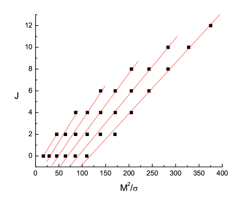
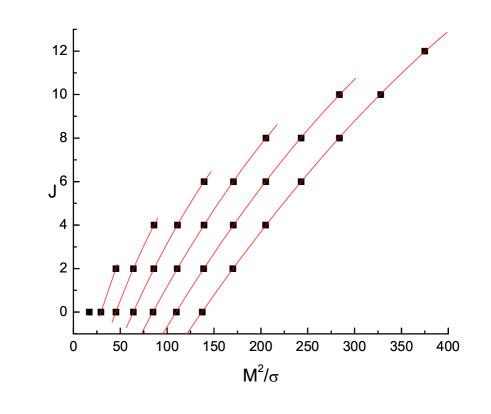
Given these generalized formulae for the masses of higher spin states, we can represent them graphically in the form of a Chew-Frautschi plot ($J$ vs. $M^{2}/\sigma$) and attempt to identify Regge trajectories. This is done in Figures $1$ and $2$. It should be noted, however, that to the best of our knowledge, there is no fundamental reason for the existence of linear Regge trajectories in the glueball sector of Yang-Mills theory. Nevertheless, our plots indicate that it is still possible to draw nearly linear Regge trajectories.

Table 8: Higher spin ($4^{++},4^{--},6^{++},6^{--},8^{++}$) glueball masses in $QCD_{3}$. All masses are in units of the square root of the string tension.

State	Our prediction
$4^{++}$	$9.27$
$4^{++*}$	$10.54$
$4^{++**}$	$11.80$
$6^{++}$	$11.81$
$6^{++*}$	$13.07$
$6^{++**}$	$14.32$
$8^{++}$	$14.33$
$8^{++*}$	$15.59$
$8^{++**}$	$16.85$
$4^{--}$	$11.32$
$4^{--*}$	$12.59$
$6^{--}$	$13.86$
$6^{--*}$	$15.12$

We would like to conclude this section by pointing out that our discussion of the mass spectrum of $2+1$ dimensional pure Yang-Mills theory is certainly not complete. In particular, current computational scheme based on the use of local probe operators is well suited for glueballs with $PC=++$ or $PC=--$. However for resonances with $PC=-+$ or $PC=+-$ any probe operator with such quantum numbers is essentially nonlocal and it is not clear at the moment how our results generalize in that case. We were able to appeal to parity doubling phenomenon to circumvent this difficulty for states of nonzero spin $J$ (although it is still interesting to compute masses of $J^{+-}$ and $J^{-+}$ directly), but for $0^{-+}$ and $0^{+-}$ we cannot do even that. It should be noted nevertheless, that it is still possible to pick certain combinations of constituent masses $M_{n}$ to approximate existing lattice data on $0^{-+}$ and $0^{+-}$, but theoretical reasons behind this are not clear.

Also we do not discuss here states of odd spin. However we would like to point out that existing lattice data for the lowest $1^{\pm+}$ states

$$\begin{array}[]{ll}M_{1^{++}}&=9.98\pm 0.5\,\sqrt{\sigma}\\ M_{1^{-+}}&=10.06\pm 0.4\,\sqrt{\sigma}\\ \end{array}$$ (94)

can be approximated (up to $5\%$) by

$$M_{1^{++}}=M_{1}+M_{1}+M_{1}+M_{2}=9.50\,\sqrt{\sigma}$$ (95)

while lattice values for $1^{\pm-}$

$$\begin{array}[]{ll}M_{1^{+-}}&=9.43\pm 0.75\,\sqrt{\sigma}\\ M_{1^{--}}&=9.36\pm 0.60\,\sqrt{\sigma}\\ \end{array}$$ (96)

should presumably correspond to

$$M_{1^{+-}}=M_{1}+M_{1}+M_{1}+M_{1}+M_{2}=11.55\,\sqrt{\sigma}.$$ (97)

As a possible explanation of such a large difference (about $20\%$) in the last case we may notice that in general it seems that $C=-$ states are heavier than $C=+$ states of the same spin (cf. $2^{++}$ and $2^{+-}$, for example). This is not the case with $1^{\pm-}$ lattice data and therefore we may question its validity.

Figure 1: Chew-Frautschi plot of the large $N$ glueball spectrum. Black boxes correspond to $J^{++}$ glueball resonances with even spins up to $J=12$. Solid red lines represent linear Regge trajectories.

Figure 2: Same data as in Figure $1$. Red lines represent polynomial data fit with second order polynomial $J=\alpha_{0}+\alpha_{1}\left(\frac{M^{2}}{\sigma}\right)+\alpha_{2}{\left(\frac{M^{2}}{\sigma}\right)}^{2}$. Note also the different way to connect data points compared to Figure $1$.

4.4 Fine Structure and Asymptotic Properties of Mass Spectrum

As was extensively discussed in previous sections, glueball masses in $2+1$-dimensional pure Yang-Mills theory are given by expressions involving zeros $\gamma_{2,i}$ of Bessel function $J_{2}(x)$. For example, equation (92) describing ${J^{++*^{n}}}$ (for even $J$) resonances can be rewritten in terms of $\gamma_{2,i}$ as

$$M_{J^{++*^{n}}}=\frac{m}{2}\left(\gamma_{2,J/2+1}+\gamma_{2,J/2+1+n}\right).$$ (98)

We can use now the following asymptotic expressions for the zeros of Bessel functions [31]

$$\gamma_{\nu,n}=\pi\left(n+\frac{1}{2}\nu-\frac{1}{4}\right)-\frac{4\nu^{2}-1}{8\pi\left(n+\frac{1}{2}\nu-\frac{1}{4}\right)}+{\cal O}\left(\frac{1}{n^{3}}\right)$$ (99)

$$\gamma_{2,n}=\pi\left(n+\frac{3}{4}\right)-\frac{15}{8\pi\left(n+\frac{3}{4}\right)}+{\cal O}\left(\frac{1}{n^{3}}\right)$$ (100)

to obtain asymptotic expressions for highly excited $J^{++*^{n}}$states (with even $J$ and large $n$):

• $$M_{0^{++*^{n}}}=m\frac{\pi}{2}\left(n+\frac{7}{4}+\frac{\gamma_{2,1}}{\pi}\right)+{\cal O}\left(\frac{1}{n}\right)$$

• $$M_{2^{++*^{n}}}=m\frac{\pi}{2}\left(n+\frac{11}{4}+\frac{\gamma_{2,2}}{\pi}\right)+{\cal O}\left(\frac{1}{n}\right)$$

• $$\ldots\ldots\ldots\ldots\ldots\ldots\ldots\ldots$$

• $$M_{J^{++*^{n}}}=m\frac{\pi}{2}\left(n+\frac{2J+7}{4}+\frac{\gamma_{2,J/2+1}}{\pi}\right)+{\cal O}\left(\frac{1}{n}\right).$$ (101)

We can see now that for large excitation level $n$, the glueball mass spectrum with given $J^{PC}$ quantum numbers becomes equidistant with mass splittings

$$\Delta M=M_{J^{++*^{(n+1)}}}-M_{J^{++*^{n}}}=m\frac{\pi}{2}.$$ (102)

For large values of spin $J$ we can further simplify Eq.(101) if we replace $\gamma_{2,J/2+1}$ by its asymptotic value. We get

$$M_{J^{++*^{n}}}=m\frac{\pi}{2}\left(n+J+\frac{7}{2}\right)+{\cal O}\left(\frac{1}{n},\frac{1}{J}\right).$$ (103)

This is an interesting expression since it tells us that there is approximate mass degeneracy in the theory. By this we mean that the mass of a state with given large values of $n$ and $J$ is approximately the same as masses of states with the corresponding excitation number and spin equal to $n+i$ and $J-i$ respectively ($i=\pm 2,\pm 4,\ldots$). Actually, since Bessel zeros approach their asymptotic values very fast we can see such approximate degeneracy even for states of low spin $J$. For example, as was found in (82) and (90) masses of $2^{++}$ and $0^{++**}$ states

$$\begin{array}[]{ll}M_{0^{++**}}&=M_{1}+M_{3}=8.38m\\ M_{2^{++}}&=M_{2}+M_{2}=8.42m\\ \end{array}$$ (104)

are very close numerically, the difference being about $.047\%$. Similarly for

$$\begin{array}[]{ll}M_{0^{++***}}&=M_{1}+M_{4}=9.97m\\ M_{2^{++*}}&=M_{2}+M_{3}=10.02m\\ \end{array}$$ (105)

the difference is about $0.52\%$.

Figure 3: “Band” structure of the mass spectrum.

We thus see that the mass spectrum of the theory has a “fine structure” with numbers of minutely separated mass eigenstates grouped together into “bands”. It is interesting nevertheless to investigate their structure a bit further. In general, $2n$’s “band” is made out of the states with the following mass content: $M_{n}+M_{n}$, $M_{n-1}+M_{n+1}$, $\ldots$, $M_{1}+M_{2n-1}$ (and similarly for “bands” with odd number $2n+1$). To see their general features, it is convenient to work out an explicit example; say, for the $50$th “band” we have

$$\begin{array}[]{c}M_{1}+M_{49}=80.70893m\\ M_{2}+M_{48}=80.77882m\\ \ldots\ldots\ldots\ldots\ldots\ldots\ldots\\ M_{23}+M_{27}=80.872686m\\ M_{24}+M_{26}=80.872792m\\ M_{25}+M_{25}=80.872827m.\\ \end{array}$$ (106)

From this example it is not difficult to see that the heaviest state within a “band” is the state with the most equal masses ($M_{25}+M_{25}$ in this example), while the lightest state is the one with the most different constituent masses ($M_{1}+M_{49}$). The “bands” do not overlap: say, the most massive state in the $49$th “band” is $M_{24}+M_{25}=79.30155m$ and so the distance between two “bands” (about $1.5m$) is about $10$ times the width of the “band” (about $0.16m$). Finally, as can be seen from (106), mass levels are very dense near the top of the “band” and spread further apart towards the bottom. Using Eq.(100) it is possible to derive the needed asymptotic expression for the mass splittings within a “band”. The highest level in the $2n$’th “band” is

$$M_{n}+M_{n}=\frac{m}{2}\left[2\pi\left(n+\frac{3}{4}\right)-\frac{30}{8\pi\left(n+\frac{3}{4}\right)}+{\cal O}\left(\frac{1}{n^{3}}\right)\right].$$ (107)

Next levels are

$$M_{n+\alpha}+M_{n-\alpha}=\frac{m}{2}\left[2\pi\left(n+\frac{3}{4}\right)-\frac{30}{8\pi\left(n+\frac{3}{4}\right)}-\frac{30}{8\pi\left(n+\frac{3}{4}\right)^{3}}\alpha^{2}+{\cal O}\left(\frac{\alpha^{4}}{n^{3}}\right)\right]$$ (108)

and therefore the distances between these levels and the highest level in the “band” are

$$\Delta M_{\alpha}=-\frac{15m}{8\pi\left(n+\frac{3}{4}\right)^{3}}\alpha^{2}+{\cal O}\left(\frac{\alpha^{4}}{n^{3}}\right)$$ (109)

for $\alpha=1,2,3...$. Figure $3$ gives graphical representation of the “band” structure.

A similar analysis can be done for states with other $J^{PC}$ quantum numbers. For brevity, we present here only the asymptotic expressions for $J^{--}$ state masses:

• $$M_{0^{--*^{n}}}=m\frac{\pi}{2}\left(n+\frac{7}{4}+\frac{\gamma_{2,1}+\gamma_{2,1}}{\pi}\right)+{\cal O}\left(\frac{1}{n}\right)$$

• $$M_{2^{--*^{n}}}=m\frac{\pi}{2}\left(n+\frac{11}{4}+\frac{\gamma_{2,1}+\gamma_{2,2}}{\pi}\right)+{\cal O}\left(\frac{1}{n}\right)$$

• $$\ldots\ldots\ldots\ldots\ldots\ldots\ldots\ldots$$

• $$M_{J^{--*^{n}}}=m\frac{\pi}{2}\left(n+\frac{2J+7}{4}+\frac{\gamma_{2,1}+\gamma_{2,J/2+1}}{\pi}\right)+{\cal O}\left(\frac{1}{n}\right).$$ (110)

and for large values of spin $J$ equation (110) further simplifies to

$$M_{J^{--*^{n}}}=m\frac{\pi}{2}\left(n+J+\frac{7}{2}+\frac{\gamma_{2,1}}{\pi}\right)+{\cal O}\left(\frac{1}{n},\frac{1}{J}\right).$$ (111)

It is interesting to note that asymptotic expressions (101) and (110) are reminiscent of empirical observations made in [29].

Also, if we include all of the spin states, the general structure appears to be reminiscent of the spectrum of a string theory. Although degeneracies are not exact, the bands that we have discussed here appear to be identifiable with the levels of a string spectrum, and there is essentially an exponentially rising density of states. This is the sense in which this theory gives a Hagedorn density of states. The fact that degeneracies are not exact, particularly at the lowest mass levels, indicates that this is not a free string theory.

5 Conclusion and Open Questions

Based on the formalism of “corner variables” [5, 7] we have presented an evaluation of a quasi-Gaussian wave functional for Yang-Mills theory in $2+1$ dimensions containing a very non-trivial kernel compatible with an infinite number of relativistic point-like resonant states. The masses of these states are all given as combinations of Bessel function zeros. The actual numerical values thus obtained are in remarkable agreement with lattice simulations [9]. The resulting picture of glueballs is based on gauge invariant constituent states, and is rather of an open-string than closed-string (Wilson loop) like nature. There are a number of outstanding technical issues, and we have been careful to point out throughout the paper the status of each step.

The perceived success is based heavily on comparisons to the existing lattice data, the most reliable of which are for the lowest lying low spin states. As one goes to higher spin states, there is certainly a lot of physical phenomena that could cloud the picture, such as the mixing of states. Although we have presented some results for non-zero spin, we should perhaps remain cautious, as there are little data to compare to. It is also possible that for some observables, the quasi-Gaussian form of the vacuum wavefunctional becomes insufficient in some way. It would be useful, for example, to construct the actual glueball wavefunctionals and compare their energies to the masses that we have derived here.

In conclusion, we believe that our results demonstrate the importance of “corner variables” [5, 7] in the pure Yang-Mills sector. As mentioned in the introduction to this paper, these variables are not only useful in $2+1$ but also in $3+1$ dimensions [8]. Many other purely theoretical questions remain: understanding of non-perturbative renormalization, better understanding of the constituent picture, exploration of the lattice formulation in terms of “corner variables”, understanding of a manifestly covariant formulation etc. Obviously on a more pragmatic level, it is important to understand the inclusion of quarks (and the emergence of mesons and baryons) in this approach in both $2+1$ and $3+1$ dimensions.

Acknowledgements

We would like to thank L. Freidel for many discussions and an illuminating collaboration. We would also like to acknowledge conversations with V. P. Nair, S. Nowling, D. Gross and T. Takeuchi, and e-mail communications from E. Witten, J. de Boer, I. Bars and especially M. Teper. We also thank numerous colleagues for raising many pertinent questions during various seminar presentations of the research contained in the present paper. RGL was supported in part by the U.S. Department of Energy under contract DE-FG02-91ER40709 and the UIUC Campus Research Board. DM and AY were supported in part by the U.S. Department of Energy under contract DE-FG05-92ER40677 and internal funds provided by Virginia Tech. Finally, we thank Perimeter Institute for hospitality.

6 Appendix A: Regulated Computations

In this Appendix we want to discuss the eigenstates of the kinetic operator

$$T=m\left(\int_{x}J^{a}(x)\frac{\delta}{\delta J^{a}(x)}+\int_{z,w}\Omega^{ab}(z,w)\frac{\delta}{\delta J^{a}(z)}\frac{\delta}{\delta J^{b}(w)}\right).$$ (112)

In particular we are interested in the action of $T$ on a special class of local operators ${\cal O}_{n}=\int\bar{\partial}J(\Delta)^{n}\bar{\partial}J$. ${\cal O}_{0}=\int\bar{\partial}J^{a}\bar{\partial}J^{a}$ has been considered previously in detail in [5] and we wish to generalize to arbitrary $n$. Since we will be unable to do this infinite number of calculations, we will focus on the general structure of $T{\cal O}_{n}$. Ultimately, we will find a number of issues in these calculations that we are unable to resolve. The issues include the use of the holomorphic invariant point-splitting regulator and precisely how to remove the regulator, as well as renormalization and normal-ordering issues. The reader should interpret this Appendix as a survey of the issues involved, as well as motivations for eq. (56); this equation is not derived.

We start with a very important technical point. The action of the operator

$$T_{1}=m\int_{x}J^{a}(x)\frac{\delta}{\delta J^{a}(x)}$$ (113)

on any local operator-valued function of $J$ is always calculationally straightforward. $T_{1}$ simply acts as a number operator counting $J$’s. For example, the action of $T_{1}$ on ${\cal O}_{0}=\int\bar{\partial}J^{a}\bar{\partial}J^{a}$ is trivial and we simply get

$$T_{1}{\cal O}_{0}=2m{\cal O}_{0}.$$ (114)

More generally though, the action of $T_{1}$ on ${\cal O}_{n}$ will not result in a holomorphic invariant.

On the other hand the action of the other part of the kinetic operator involving

$$T_{2}=m\int_{z,w}\Omega^{ab}(z,w)\frac{\delta}{\delta J^{a}(z)}\frac{\delta}{\delta J^{b}(w)}$$ (115)

is very subtle. For ${\cal O}_{0}$ we have

$$\frac{\delta^{2}{\cal O}_{0}}{\delta J^{a}(z)\delta J^{b}(w)}=-2\,\delta^{ab}\,{\bar{\partial}}_{z}^{2}\delta(z-w)$$ (116)

and so

$$T_{2}{\cal O}_{0}=-2m\int_{w}\delta^{ab}\left[{\bar{\partial}}_{z}^{2}\Omega^{ab}(z,w)\right]_{z=w}.$$ (117)

To compute the right-hand side of Eq.(117), we use the point-split expression for $\Omega^{ab}(z,w)$ [5]

$$\Omega^{ab}(z,w)=D_{w}^{br}\Lambda_{ra}(w,z)$$ (118)

where $D_{w}^{br}$ is the adjoint representation of the holomorphic-covariant derivative, and [5]

$$\Lambda_{ra}(w,z)=\frac{1}{\pi(z-w)}\left[\delta_{ra}-{\left(H(w)H^{-1}(z,\bar{w})\right)}_{ra}e^{-\frac{\alpha}{2}}\right]+...$$ (119)

with $\alpha\equiv\frac{|z-w|^{2}}{\epsilon}$, and $\epsilon\to 0$. Now one easily obtains (summation over repeated index is understood)

$$\left[{\bar{\partial}}_{z}^{2}\Omega^{aa}(z,w)\right]_{z=w}=\frac{c_{A}}{\pi}\frac{(dim\,G)}{4\pi\epsilon^{2}}$$ (120)

and finally

$$T_{2}\,{\cal O}_{0}=-m\int\frac{c_{A}}{\pi}\frac{(dim\,G)}{2\pi\epsilon^{2}}.$$ (121)

From this we see that the only effect of $T_{2}$ acting on ${\cal O}_{0}$ is to give a divergent normal-ordering correction. We may now define

$$:\!{\cal O}_{0}\!:\ =\int\left[\bar{\partial}J^{a}\bar{\partial}J^{a}-\frac{c_{A}}{\pi}\frac{(dim\,G)}{4\pi\epsilon^{2}}\right]$$ (122)

and for normal-ordered operator $:\!{\cal O}_{0}\!:$ we get

$$T\,:\!{\cal O}_{0}\!:\ =2m:\!{\cal O}_{0}\!:.$$ (123)

In what follows we will not keep track of such divergent terms explicitly, however it should be understood that the rest of ${\cal O}_{n}$ operators have to be normal-ordered in a similar way.

Let us proceed now to the operator

$${\cal O}_{1}=\int\bar{\partial}J^{a}(\Delta)^{ab}\bar{\partial}J^{b}=\int\bar{\partial}J^{a}D^{ab}\,\bar{\partial}^{2}\!J^{b}.$$ (124)

The action of $T_{1}$ on this is elementary

$$T_{1}\,{\cal O}_{1}=2m\int\bar{\partial}J^{a}(\partial)\,\bar{\partial}^{2}\!J^{a}+3m\int\bar{\partial}J^{a}\left(-i\frac{\pi}{c_{A}}f^{adb}J^{d}\right)\bar{\partial}^{2}J^{b}.$$ (125)

Note however that this result is not invariant under holomorphic transformations. What we want to show now is that when $T_{2}$ acts on the $3J$-part of ${\cal O}_{1}$ (the action on the $2J$-part is trivial and gives only a normal-ordering constant as was discussed above) it generates an extra term with two $J$’s which restores holomorphic invariance, i.e.

$$T_{2}\,{\cal O}_{1}=m\int\bar{\partial}J^{a}(\partial)\,\bar{\partial}^{2}\!J^{a}$$ (126)

and therefore

$$T\,{\cal O}_{1}=(T_{1}+T_{2})\,{\cal O}_{1}=3m\,{\cal O}_{1}.$$ (127)

But before we proceed to show that (126) is correct we want to make a technical remark which will significantly simplify calculations. As can be seen from expressions (118) and (119) every time $\bar{\partial}_{z}$ acts on $\Omega^{ab}(z,w)$ it actually acts on the exponent in $\Lambda_{ra}$ and thus pulls out a factor $1/\epsilon$. Therefore expressions like $\left[{\bar{\partial}}_{z}\Omega^{ab}(z,w)\right]_{z=w}$, $\left[{\bar{\partial}}_{z}\partial_{w}\Omega^{ab}(z,w)\right]_{z=w}$, etc will lead to divergent normal-ordering terms only (cf. Eq.(120), for example). Such expressions will appear when $\delta/\delta J^{a}(z)$ partial derivative acts on $J$’s with leading antiholomorphic derivatives, like $\bar{\partial}J$ or $\bar{\partial}^{2}\!J$ in the case of ${\cal O}_{1}$ operator. Therefore, as long as we are not interested in explicit form of the normal-ordering terms, we can consider action of $\delta/\delta J^{a}(z)$ on “bare” $J$’s only. Therefore

$$\frac{\delta{\cal O}_{1}}{\delta J^{a}(z)}=\left(-i\frac{\pi}{c_{A}}f^{dae}\right)\,\bar{\partial}J^{d}_{z}\,{\bar{\partial}}^{2}\!J^{e}_{z}$$ (128)

and

$$\frac{\delta{\cal O}_{1}}{\delta J^{a}(z)\delta J^{b}(w)}=\left(-i\frac{\pi}{c_{A}}f^{bae}\right)\left({\bar{\partial}}^{2}\!J^{e}_{z}\>\bar{\partial}_{z}\delta(z-w)-{\bar{\partial}}J^{e}_{z}\>{\bar{\partial}}_{z}^{2}\delta(z-w)\right)$$ (129)

from which we immediately obtain

$$T_{2}\,{{\cal O}_{1}}=m\int\left(-i\frac{\pi}{c_{A}}f^{bae}\right)\left({\bar{\partial}}^{2}\!J^{e}\left[{\bar{\partial}}_{w}\Omega^{ab}(z,w)\right]_{z=w}-\ {\bar{\partial}}J^{e}\left[{\bar{\partial}}_{w}^{2}\Omega^{ab}(z,w)\right]_{z=w}\right).$$ (130)

To proceed further we need to evaluate $\left[{\bar{\partial}}_{w}\Omega^{ab}(z,w)\right]_{z=w}$ and $\left[{\bar{\partial}}_{w}^{2}\Omega^{ab}(z,w)\right|_{z=w}$. A straightforward computation gives (we keep only finite terms which do not depend on regularization parameter $\epsilon$)

$$\left[{\bar{\partial}}_{w}\Omega^{ab}(z,w)\right]_{z=w}=\frac{1}{2\pi}\,\bar{\partial}\!\left(DJ\right)^{ba}=\frac{1}{2\pi}\,\partial\bar{\partial}J^{ba}-\frac{1}{2\pi}\frac{\pi}{c_{A}}\,\bar{\partial}\!\left(JJ\right)^{ba}$$ (131)

$$\left[{\bar{\partial}}_{w}^{2}\Omega^{ab}(z,w)\right]_{z=w}=\frac{1}{2\pi}\,{\bar{\partial}}^{2}\!\!\left(DJ\right)^{ba}=\frac{1}{2\pi}\,\partial{\bar{\partial}}^{2}\!J^{ba}-\frac{1}{2\pi}\frac{\pi}{c_{A}}\,{\bar{\partial}}^{2}\!\!\left(JJ\right)^{ba}$$ (132)

and

$$T_{2}\,{{\cal O}_{1}}=m\int\left(-i\frac{1}{2c_{A}}f^{bae}\right)\left({\bar{\partial}}^{2}\!J^{e}\>\partial\bar{\partial}J^{ba}-\ {\bar{\partial}}J^{e}\>\partial{\bar{\partial}}^{2}\!J^{ba}\right).$$ (133)

Finally, we may use the identity $f^{bae}J^{ba}=ic_{A}\,J^{e}$ to verify that (133) is indeed equivalent to (126).

To summarize, what we have shown is that the action of kinetic energy operator on ${\cal O}_{1}$ gives a gauge and holomorphic invariant result

$$T\,:{\cal O}_{1}:=3m\,:{\cal O}_{1}:.$$ (134)

Finally, let us consider one further example

$${\cal O}_{2}=\int\bar{\partial}J^{a}(\Delta^{2})^{ab}\,\bar{\partial}J^{b}.$$ (135)

It is convenient to rewrite this as

$${\cal O}_{2}=\int(D\,{\bar{\partial}}^{2}\!J)^{d}(D\,{\bar{\partial}}^{2}\!J)^{d}.$$ (136)

Proceeding now the same way as we did for ${\cal O}_{1}$, we obtain

$$\frac{\delta{\cal O}_{2}}{\delta J^{a}(z)}=2\,\frac{\pi}{c_{A}}\left(-if^{dac}\,{\bar{\partial}}^{2}\!J^{c}_{z}\right)\,\left(D\,{\bar{\partial}}^{2}\!J\right)^{d}_{z}$$ (137)

and

$$\frac{\delta{\cal O}_{2}}{\delta J^{a}(z)\delta J^{b}(w)}=2\,\frac{\pi}{c_{A}}\>\biggl{\{}\left(-if^{dab}\>{\bar{\partial}}^{2}_{z}\delta(z-w)\right)\left(D\,{\bar{\partial}}^{2}\!J\right)^{d}_{z}+\qquad\qquad\$$ (138)

$$\left(-if^{dac}\>{\bar{\partial}}^{2}\!J^{c}_{z}\right)\left(D^{db}_{z}\,{\bar{\partial}}^{2}_{z}\delta(z-w)\right)+\qquad\quad\ \,$$

$$\left(-if^{dac}\>{\bar{\partial}}^{2}\!J^{c}_{z}\right)\frac{\pi}{c_{A}}\,\delta(z-w)\left(-if^{dbe}\>{\bar{\partial}}^{2}\!J^{e}_{z}\right)\biggr{\}}.$$

Now we may write for the action of $T_{2}$ on ${\cal O}_{2}$

$$T_{2}{\cal O}_{2}=2m\frac{\pi}{c_{A}}\>\biggl{\{}\int\left(-if^{dab}\left[{\bar{\partial}}^{2}_{w}\Omega^{ab}(z,w)\right]_{z=w}\right)\left(D\,{\bar{\partial}}^{2}\!J\right)^{d}+\qquad\quad\ \ \ \ \!$$ (139)

$$\int\left(-if^{dac}\>{\bar{\partial}}^{2}\!J^{c}\right)\left(\left[D^{db}_{w}\,{\bar{\partial}}^{2}_{w}\Omega^{ab}(z,w)\right]_{z=w}\right)+\qquad\quad\$$

$$\int\left(-if^{dac}\>{\bar{\partial}}^{2}\!J^{c}\right)\frac{\pi}{c_{A}}\left[\Omega^{ab}(z,w)\right]_{z=w}\left(-if^{dbe}\>{\bar{\partial}}^{2}\!J^{e}\right)\biggr{\}}.$$

Since $\left[{\bar{\partial}}^{2}_{w}\Omega^{ab}(z,w)\right]_{z=w}$ was computed previously in (132), we immediately obtain for the first term in (139)

$$2m\,\frac{\pi}{c_{A}}\int\left(-if^{dab}\left[{\bar{\partial}}^{2}_{w}\Omega^{ab}(z,w)\right]_{z=w}\right)\left(D\,{\bar{\partial}}^{2}\!J\right)^{d}_{z}\ =\ m\int\left(\partial{\bar{\partial}}^{2}\!J\right)^{d}\left(D\,{\bar{\partial}}^{2}\!J\right)^{d}.$$ (140)

Similarly for the last term in (139) we need expression for $\left[\Omega^{ab}(z,w)\right]_{z=w}$ which is

$$\left[\Omega^{ab}(z,w)\right]_{z=w}=\frac{1}{2\pi}\left(DJ\right)^{ba}=\frac{1}{2\pi}\partial J^{ba}-\frac{1}{2\pi}\frac{\pi}{c_{A}}\left(JJ\right)^{ba}$$ (141)

and therefore

$$2m\left(\frac{\pi}{c_{A}}\right)^{2}\!\!\int\left(-if^{dac}\>{\bar{\partial}}^{2}\!J^{c}_{z}\right)\left[\Omega^{ab}(z,w)\right]_{z=w}\left(-if^{dbe}\>{\bar{\partial}}^{2}\!J^{e}_{z}\right)=-m\frac{1}{\pi}\left(\frac{\pi}{c_{A}}\right)^{2}\!\!\int\left({\bar{\partial}}^{2}\!J{\bar{\partial}}^{2}\!JDJ\right)^{aa}$$ (142)

where summation over the repeated index $a$ on the right-hand side of this expression is implied (this essentially amounts to taking trace in adjoint representation). Finally, for the second term in (139) we will need

$$\left[D^{db}_{w}\,{\bar{\partial}}^{2}_{w}\Omega^{ab}(z,w)\right]_{z=w}=\frac{1}{2\pi}\left\{D{\bar{\partial}}^{2}DJ-\frac{1}{3}{\bar{\partial}}^{2}D^{2}J\right\}^{da}$$ (143)

from which we obtain

$$2m\frac{\pi}{c_{A}}\int\left(-if^{dac}\>{\bar{\partial}}^{2}\!J^{c}_{z}\right)\left(\left[D^{db}_{w}\,{\bar{\partial}}^{2}_{w}\Omega^{ab}(z,w)\right]_{z=w}\right)=-\frac{m}{c_{A}}\int\left({\bar{\partial}}^{2}J\left\{D{\bar{\partial}}^{2}DJ-\frac{1}{3}{\bar{\partial}}^{2}D^{2}J\right\}\right)^{aa}.$$ (144)

Now if we collect all the results in equations (140), (142) and (144) together and after some simple but somewhat lengthy transformations we obtain the final expression for the action of $T_{2}$ operator on ${\cal O}_{2}$ state

$$T_{2}\,{\cal O}_{2}=\frac{m}{3}\,\biggl{\{}5\int\left(\partial{\bar{\partial}}^{2}\!J\right)^{a}\left(\partial{\bar{\partial}}^{2}\!J\right)^{a}-\qquad\qquad\quad\$$ (145)

$$4\int\left(\partial{\bar{\partial}}^{2}\!J\right)^{a}\left(\frac{\pi}{c_{A}}\,[J,{\bar{\partial}}^{2}\!J]\right)^{a}-\>\,\qquad$$

$$\int\left(\frac{\pi}{c_{A}}\,[J,{\bar{\partial}}^{2}\!J]\right)^{a}\left(\frac{\pi}{c_{A}}\,[J,{\bar{\partial}}^{2}\!J]\right)^{a}-\!\!\!$$

$$\int\frac{\pi}{c_{A}}\left([\bar{\partial}J,{\bar{\partial}}^{2}J]\right)^{d}\left(D\bar{\partial}J\right)^{d}\biggr{\}}\quad\qquad$$

which combined with the straightforward result for $T_{1}{\cal O}_{2}$

$$T_{1}\,{\cal O}_{2}=m\,\biggl{\{}2\int\left(\partial{\bar{\partial}}^{2}\!J\right)^{a}\left(\partial{\bar{\partial}}^{2}\!J\right)^{a}-\qquad\qquad\quad\ \,$$ (146)

$$6\int\left(\partial{\bar{\partial}}^{2}\!J\right)^{a}\left(\frac{\pi}{c_{A}}\,[J,{\bar{\partial}}^{2}\!J]\right)^{a}+\qquad\ \>$$

$$4\int\left(\frac{\pi}{c_{A}}\,[J,{\bar{\partial}}^{2}\!J]\right)^{a}\left(\frac{\pi}{c_{A}}\,[J,{\bar{\partial}}^{2}\!J]\right)^{a}\biggr{\}}$$

finally gives

$$T\,{\cal O}_{2}=\left(4-\frac{1}{3}\right)m{\cal O}_{2}+\frac{m}{3}\frac{\pi}{c_{A}}\int\left([\bar{\partial}J,{\bar{\partial}}^{2}J]\right)^{d}\left(D\bar{\partial}J\right)^{d}.$$ (147)

As a consistency check one may notice that we obtain a gauge and holomorphically invariant expression as expected.

A few comments about this result are in order, as it is not of the form that we have expected. First of all we see that an extra gauge invariant operator $\int\left([\bar{\partial}J,{\bar{\partial}}^{2}J]\right)^{d}\left(D\bar{\partial}J\right)^{d}$ mixes with ${\cal O}_{2}$. Such operator mixing is certainly expected to be the general feature of the theory and therefore we may write

$$T{\cal O}_{n}=E_{n}{{\cal O}}_{n}+\ldots$$ (148)

where “$\ldots$” indicate operators which mix with ${\cal O}_{n}$ under the action of $T$. It should be noted, however, that such operators, even though they have the same mass dimension as ${\cal O}_{n}$, are of higher order in $\bar{\partial}J$. By this we mean that only ${\cal O}_{n}$ in equation (148) contains terms quadratic in $\bar{\partial}J$ while the rest of the operators have at least three $\bar{\partial}J$’s. This means, in particular, that such operator mixing has no influence on derivation of Schrödinger equation presented in this paper and therefore detailed knowledge of “$\ldots$” terms in equation (148) is not really necessary for our purposes.

More worrisome is the numerical coefficient of ${{\cal O}}_{2}$ in (147). As can be seen from (147), we may think of ${\cal O}_{2}$ as an eigenstate (up to an extra operator that mixes in) of kinetic energy with eigenvalue $(4-1/3)m$.

We believe, however, that this result is not complete and the correct spectrum for the kinetic energy should be equidistant

$$T{\cal O}_{n}=(n+2)m{\cal O}_{n}+\ldots.$$ (149)

The reason why we have not obtained the expected answer in the case of ${\cal O}_{2}$ (and presumably for ${\cal O}_{n>2}$) may be that we have not taken proper account of the nonlocal character of the theory. Thus the calculation that we have outlined above needs to be reconsidered carefully. We do not at this time have a consistent understanding of all of these issues as the required calculations are tedious, but we present remarks below. In the text of the paper, we use eq. (149) without further apologies.

6.1 Further discussion: regulator/renormalization issues

In deriving results for ${\cal O}_{0}$, ${\cal O}_{1}$ and ${\cal O}_{2}$ operators we have been using expression for $\Omega^{ab}(z,w)$ with $\Lambda_{ra}(w,z)$ given in equation (119). This expression for $\Lambda_{ra}(w,z)$ is in fact a simplified form of the exact regulator [5]

$$\Lambda_{ra}(w,z)=\frac{1}{\pi(z-w)}\left[\delta_{ra}-{\left(H(w)H^{-1}(u,\bar{w})H(u)H^{-1}(z,\bar{u})\right)}_{ra}e^{-\frac{\alpha}{2}}\right]+...$$ (150)

where $u=\frac{1}{2}(z+w)$ and $\bar{u}=\frac{1}{2}(\bar{z}+\bar{w})$. It is easy to see that (119) can be obtained from this expression if we put $\bar{z}=\bar{w}$ in ${\left(H(w)H^{-1}(u,\bar{w})H(u)H^{-1}(z,\bar{u})\right)}_{ra}$ . Therefore (119) is equivalent to (150) up to the $O(\bar{z}-\bar{w})$ terms. Part of the problem uncovered in the previous section then may have to do with subtleties involving the assumed form of $\Lambda_{ra}$. It seems that for the study of the action of $T_{2}$ on local operators, such simplification is not justified and exact expression (150) should be used. Although it becomes extremely difficult to do calculations with this $\Lambda_{ra}(w,z)$, we have considered this effect on ${\cal O}_{0}$ and ${\cal O}_{1}$. There appear to be additional contributions (of the form $\epsilon/\epsilon$) even to their eigenvalues

$$T\,{\cal O}_{0}\sim 2\left(1-\frac{1}{16}\right)m{\cal O}_{0}$$ (151)

$$T\,{\cal O}_{1}\sim 3\left(1-\frac{3}{32}\right)m{\cal O}_{1}.$$

What does this effect illustrate? There are certainly very subtle effects coming from the point-splitting regulator. We have not been able to arrive at a consistent method for dealing with these effects. In addition though, we should note that these are all formal expressions – we have not carefully defined the operators or the coupling, particularly in the infrared. It is not clear to us that such a procedure is known in this or any other (non-trivial) theory.

Let us be a little more explicit about the issue raised here. In performing computations for ${\cal O}_{0}$, ${\cal O}_{1}$ and ${\cal O}_{2}$ we have kept track of $\epsilon$-independent terms only. In general, however, we may write

$$\begin{array}[]{c}T\,{\cal O}_{0}=\ldots+T_{00}\,{\cal O}_{0}+T_{10}\,\epsilon\,{\cal O}_{1}+T_{20}\,\epsilon^{2}\,{\cal O}_{2}+\ldots\\ T\,{\cal O}_{1}=\ldots+T_{11}\,{\cal O}_{1}+T_{21}\,\epsilon\,{\cal O}_{2}+T_{31}\,\epsilon^{2}\,{\cal O}_{3}+\ldots\\ T\,{\cal O}_{2}=\ldots+T_{22}\,{\cal O}_{2}+T_{32}\,\epsilon\,{\cal O}_{3}+T_{42}\,\epsilon^{2}\,{\cal O}_{4}+\ldots\\ \ldots\ldots\ldots\ldots\ldots\ldots\ldots\ldots\ldots\end{array}$$ (152)

or in matrix notation

$$T\,{\cal O}_{i}=T_{ji}\,\epsilon^{j-i}\,{\cal O}_{j}.$$ (153)

This is a schematic expression based solely on dimensional analysis (remember that $[{\cal O}_{n}]={\rm(mass)}^{4+2n}$). It does not include, for example, the effects of mixing with operators other than ${\cal O}_{n}$. $T_{ij}$ here is an infinite dimensional number matrix which can be thought of as a representation of kinetic energy operator in the basis provided by operators ${\cal O}_{n}$. Evaluating the spectrum of $T$ would then certainly amount to diagonalizing $T_{ij}$. In some sense what we have done above is have found diagonal elements $T_{nn}$ of this matrix and associated them with the spectrum of kinetic operator. In other words if one takes naive $\epsilon\to 0$ limit in (152) it looks like all terms with positive powers of $\epsilon$ go to zero, $T_{ij}$ matrix becomes triangular and, consequently, diagonal elements give the spectrum. The proper procedure, however, would be to diagonalize $T_{ij}$ first and take $\epsilon\to 0$ limit afterwards. Formally we may write the $n$-th eigenstate as a linear combination of an infinite number of local operators ${\cal O}_{n}$

$$Q^{(n)}=c^{(n)}_{i}\,\epsilon^{i-n}\,{\cal O}_{i}$$ (154)

with some unknown numeric coefficients $c^{(n)}_{i}$. The eigenvalue equation

$$T\,{\cal Q}^{(n)}=E^{(n)}{\cal Q}^{(n)}$$ (155)

becomes now the infinite-dimensional matrix equation

$$T_{ji}\,c^{(n)}_{i}=E^{(n)}\,c^{(n)}_{j}$$ (156)

from which in principle we could find the spectrum. Of course, to do this practically would be a very difficult task. Note, however, that the $\epsilon$-dependence completely drops out from this expression. This means, in particular, that the spectrum of $T$ does not depend on the regularization parameter $\epsilon$ and we may take the formal limit $\epsilon\to 0$ in (154) after diagonalization. At any finite value of $\epsilon$ the true eigenstates ${\cal Q}^{(n)}$ of $T$ are certainly nonlocal, however we expect that they will collapse into local states as $\epsilon\to 0$, i.e.

$${\cal Q}^{(n)}\stackrel{{\scriptstyle\epsilon\to\,0}}{{\longrightarrow}}\ :\!{\cal O}_{n}\!:.$$ (157)

Therefore for any practical purposes, like writing Schrödinger equation for the full Hamiltonian ${\cal H}$, we may think of the eigenstates of kinetic energy in terms of local operators $:\!{\cal O}_{n}\!:$ and we may now really write

$$T\,:\!{\cal O}_{n}\!:\stackrel{{\scriptstyle\epsilon\to 0}}{{=}}E^{(n)}:\!{\cal O}_{n}\!:+\ldots$$ (158)

It should be noted however that this expression, even though it looks completely local, knows in fact about nonlocal character of the theory. This nonlocal information is contained in the spectrum $E^{(n)}$ which should be obtained by solving eigenvalue equations with nonlocal ansatz (154).

To conclude this discussion, we would like to consider a simple example which further illustrates the intuitive arguments presented above. In [5] the following nonlocal generalization of ${\cal O}_{0}$ was proposed

$${\cal Q}^{(0)}_{\epsilon}=\int_{x,y}\frac{e^{-\frac{|x-y|^{2}}{\epsilon}}}{\pi\epsilon}\ \bar{\partial}J^{a}(x)\left[H(x,\bar{y})H^{-1}(y)\right]^{ab}\bar{\partial}J^{a}(x).$$ (159)

This state is essentially made of two $\bar{\partial}J$’s connected by a straight Wilson line. It is not difficult now to expand this in terms of local operators with the result given by

$${\cal Q}^{(0)}_{\epsilon}={\cal R}_{0}+\epsilon{\cal R}_{1}+\frac{1}{2!}\epsilon^{2}{\cal R}_{2}+\frac{1}{3!}\epsilon^{3}{\cal R}_{3}+\ldots$$ (160)

where

$${\cal R}_{n}=\int\bar{\partial}J^{a}\left(D^{n}{\bar{\partial}}^{n}\right)^{ab}\bar{\partial}J^{b}.$$ (161)

These ${\cal R}_{n}$ operators are not quite the same as ${\cal O}_{n}$ (except ${\cal R}_{0}\equiv{\cal O}_{0}$ and ${\cal R}_{1}\equiv{\cal O}_{1}$), however they coincide with the latter to quadratic order in $J$. Therefore from this expansion we see that ${\cal Q}^{(0)}_{\epsilon}$ is of the same type as we need to diagonalize $T$ according to (154). Of course, this simple operator is not an eigenstate of $T$, however we may see the other essential ingredient of the above analysis, namely the fact that in the continuum $\epsilon\to 0$ limit, ${\cal Q}^{(0)}_{\epsilon}$ collapses into local operator ${\cal O}_{0}$.

7 Appendix B: Vacuum Energy

Here we discuss the vacuum energy. For this purpose, we need to evaluate the Schrödinger equation in the form

$${\cal H}_{KN}\Psi_{0}=(E_{0}+\ldots)\Psi_{0}$$ (162)

where $E_{0}$ consists of terms that survive as $J^{a}\to 0$. Since the Hamiltonian involves at most two derivatives with respect to $J$, we can drop any $J$-dependence of the kernel for this computation and work with

$$\Psi_{0}\simeq{\rm exp}\left({-\frac{\pi}{2c_{A}m^{2}}\int\bar{\partial}J^{a}K[\partial\bar{\partial}/m^{2}]\bar{\partial}J^{a}}\right).$$ (163)

We then compute

$$\frac{\delta}{\delta J^{a}(z)}\Psi_{0}=\frac{\pi}{c_{A}m^{2}}\left(\bar{\partial}\,K\!\left[\partial\bar{\partial}/m^{2}\right]\bar{\partial}J\right)^{a}_{z}\Psi_{0}$$ (164)

and

$$\frac{\delta^{2}}{\delta J^{b}(w)\delta J^{a}(z)}\Psi_{0}=\frac{\pi}{c_{A}m^{2}}\,\left(K\!\left[\partial\bar{\partial}/m^{2}\right]\!\bar{\partial}^{2}\right)_{z}\delta^{(2)}(z-w)\delta^{ab}\Psi_{0}+\ldots$$ (165)

and so

$$m\int_{w,z}\Omega^{ab}(z,w)\frac{\delta^{2}}{\delta J^{b}(w)\delta J^{a}(z)}\Psi_{0}=\left(\int_{z}{\cal E}_{0}+\ldots\right)\Psi_{0}.$$ (166)

We then deduce that the vacuum energy density is

$${\cal E}_{0}=\frac{\pi}{c_{A}m}\,\delta_{ab}\left.\left(K\!\left[\partial\bar{\partial}/m^{2}\right]{\bar{\partial}}^{2}\right)_{z}\Omega^{ab}(z,w)\right|_{w=z}.$$ (167)

To proceed, we write out the regulated $\Omega^{ab}$ keeping only those terms that are present in the $J^{a}\to 0$ limit. This is particularly simple, and we find

$$\Omega^{ab}_{reg}(z,w)=\frac{c_{A}}{\pi}(D_{w}\Lambda(w,z))^{ba}=\frac{c_{A}}{\pi}\,\delta^{ab}\,\partial_{w}\frac{1}{\pi(z-w)}\left(1-e^{-|z-w|^{2}/2\epsilon}\right).$$ (168)

In the expression for the vacuum energy, there is a leading $\bar{\partial}_{z}^{2}$; performing one of these derivatives on $\Omega^{ab}_{reg}$, we find

$${\cal E}_{0} = \frac{dim\,G}{m}\left.\left(K\!\left[\partial\bar{\partial}/m^{2}\right]{\bar{\partial}}\right)_{z}\partial_{w}\frac{1}{2\pi\epsilon}e^{-|z-w|^{2}/2\epsilon}\right|_{w=z}$$ (169)

$$= -m(dim\,G)\ \left.\left(K\!\left[\frac{\partial\bar{\partial}}{m^{2}}\right]\frac{\partial\bar{\partial}}{m^{2}}\right)_{z}\frac{1}{2\pi\epsilon}e^{-|z-w|^{2}/2\epsilon}\right|_{w=z}.$$

This expression is horribly divergent. Let us proceed however by considering the expansion for $K$

$$K[x]\,x=\sum_{n=0}^{\infty}c_{n}x^{n+1}.$$ (170)

We then find

$${\cal E}_{0}=-\frac{(dim\,G)\ m}{2\pi\epsilon}\sum_{n=0}^{\infty}c_{n}(n+1)!\left(-\frac{1}{2\epsilon m^{2}}\right)^{n+1}.$$ (171)

Note that the appearance of divergences to arbitrary order here comes directly from the fact that the vacuum wave-functional contains operators of arbitrarily high dimension. This basic fact plagues all such computations. In the case of the vacuum energy, it is possible to resum this series and extract sensible results (in particular, the asymptotic behavior is consistent with the UV perturbation theory). The basic observation is that

$$(n+1)!\ t^{-2-n}=\int_{0}^{\infty}dx\ x^{n+1}e^{-tx}$$ (172)

and so we have

$${\cal E}_{0} = \frac{(dim\,G)\ m^{3}}{\pi}\sum_{n=0}^{\infty}c_{n}(-1)^{n}\left.\int_{0}^{\infty}dx\ x^{n+1}e^{-tx}\right|_{t=2\epsilon m^{2}}$$ (173)

$$= \frac{(dim\,G)\ m^{3}}{\pi}\left.\int_{0}^{\infty}dx\ xK(-x)e^{-tx}\right|_{t=2\epsilon m^{2}}.$$

Thus the vacuum energy may be written as the Laplace transform of $xK(-x)$. Removing the regulator corresponds to taken the asymptotic $t=2\epsilon m^{2}\to 0$ limit.

7.1 Evaluation of ${\cal E}_{0}$

To proceed further, we need to supply information about $K$. We will consider several examples, culminating with the kernel (62).

7.1.1 $K\equiv 1$

The simplest choice is to consider $K\equiv 1$, which corresponds to replacing the true $K$ by its IR limit. In this case, the Laplace transform is elementary, and we obtain

$${\cal E}^{K\equiv 1}_{0}=\frac{dim\,G}{4\pi m\epsilon^{2}}$$ (174)

which is quartically divergent (in powers of a momentum cutoff).

7.1.2 Massless Boson

If we consider the wavefunctional corresponding to a free massless boson, we have $K(-x)=1/\sqrt{x}$. Again, the Laplace transform is elementary, and we obtain

$${\cal E}^{particle}_{0}=\frac{dim\,G}{4\sqrt{2\pi}\epsilon^{3/2}}.$$ (175)

This is also the UV limit of the true $K$; we see here that the scale $m$ drops out of this result, as it should.

7.1.3 Bessel

Finally, let us consider the kernel (62). $K(-x)$ can be written as

$$K(-x)=\frac{1}{\sqrt{x}}\frac{I_{2}(4\sqrt{x})}{I_{1}(4\sqrt{x})}$$ (176)

and so we need to compute

$${\cal E}^{YM}_{0}=\frac{(dim\,G)\ m^{3}}{\pi}\int_{0}^{\infty}dx\ \sqrt{x}\,\frac{I_{2}(4\sqrt{x})}{I_{1}(4\sqrt{x})}\,e^{-tx}.$$ (177)

Because we are interested in the small $t$ limit, it is sufficient to consider the asymptotic $x\to\infty$ behavior of the integrand

$$\sqrt{x}\frac{I_{2}(4\sqrt{x})}{I_{1}(4\sqrt{x})}\simeq\sqrt{x}-\frac{3}{8}+\frac{3}{128}\frac{1}{\sqrt{x}}+{\cal O}(1/x).$$ (178)

We thus obtain

$${\cal E}^{YM}_{0}=\frac{dim\ G}{4\sqrt{2\pi}\epsilon^{3/2}}\left[1-\frac{3m\sqrt{\epsilon}}{2\sqrt{2\pi}}+\frac{3m^{2}\epsilon}{32}\right]+{\cal O}(m^{3}\log(\epsilon m)).$$ (179)

Note that the leading divergence is the same as the UV result, while the subleading terms depend on the detailed form of the kernel.

8 Appendix C: Vacuum Solutions

Assuming the validity of the Riccati equation (59)

$$-K-\frac{L}{2}\frac{d}{dL}[K(L)]+LK^{2}+1=0$$ (180)

we now consider its general solution. This is a non-linear differential equation but it is easily solved by substituting $K=-y^{\prime}/2y$ to obtain

$$Ly^{\prime\prime}+2y^{\prime}+4y=0.$$ (181)

Then, writing $y=f(x)/\sqrt{L}$ with $x=4\sqrt{L}$ leads to the Bessel equation

$$f^{\prime\prime}(x)+f^{\prime}(x)/x+(1-1/x^{2})f(x)=0$$ (182)

with general solution

$$y=c_{1}\frac{1}{\sqrt{L}}J_{1}(4\sqrt{L})+c_{2}\frac{1}{\sqrt{L}}Y_{1}(4\sqrt{L}).$$ (183)

Using the standard recursive formulae (with similar formulae for $Y_{\nu}$)

$$\begin{array}[]{ccl}J_{\nu-1}(u)+J_{\nu+1}(u)&=&\frac{2\nu}{u}J_{\nu}(u)\\ &&\\ J_{\nu-1}(u)-J_{\nu+1}(u)&=&2J^{\prime}_{\nu}(u)\end{array}$$ (184)

the general solution of (180) takes the form

$$K(L)=\frac{1}{\sqrt{L}}\frac{CJ_{2}(4\sqrt{L})+Y_{2}(4\sqrt{L})}{CJ_{1}(4\sqrt{L})+Y_{1}(4\sqrt{L})}.$$ (185)

Here we have a one-parameter family of solutions, parameterized by $C$. The solution quoted in the text (62) corresponds to $C\to\infty$. To see why we should take this value, we study the asymptotics of the solutions, paying close attention to the normalizability of the solution. It is particularly satisfying that the only normalizable solution corresponds to the confining vacuum.

To study the asympotics, we note that $L=\partial\bar{\partial}/m^{2}\to-k^{2}/4m^{2}$ is negative (choice of square root doesn’t matter), and so we need the identities

$$J_{1}(iz)=iI_{1}(z),\ \ \ \ J_{2}(iz)=-I_{2}(z),$$

$$Y_{1}(iz)=-I_{1}(z)+\frac{2i}{\pi}K_{1}(z),\ \ \ \ Y_{2}(iz)=-iI_{2}(z)+\frac{2}{\pi}K_{2}(z)$$ (186)

giving

$$K(-|L|)=\frac{1}{\sqrt{|L|}}\frac{C^{\prime}I_{2}(4\sqrt{|L|})-K_{2}(4\sqrt{|L|})}{C^{\prime}I_{1}(4\sqrt{|L|})+K_{1}(4\sqrt{|L|})}$$ (187)

where $C^{\prime}=\pi(C+i)/2$. We will consider real $C^{\prime}$ in what follows (this corresponds to real wavefunctionals), but this is not a crucial simplification: the final conclusion will be unchanged.

Now, asymptotically $|L|\to\infty$, this function behaves differently, depending on whether $C^{\prime}=0$ or not, because only for that value of $C^{\prime}$ will the $K_{n}$’s play a role:

$$K(-|L|)\ \begin{subarray}{c}|L|\to\infty\\ \longrightarrow\end{subarray}\left\{\begin{array}[]{rl}+\frac{1}{\sqrt{|L|}},&for\ |C^{\prime}|\neq 0\cr-\frac{1}{\sqrt{|L|}},&for\ |C^{\prime}|=0.\end{array}\right.$$ (188)

For small $|L|$ on the other hand, the $K_{n}$’s will dominate, unless $C^{\prime}\to\pm\infty$. Thus we find

$$K(-|L|)\ \begin{subarray}{c}|L|\to 0\\ \longrightarrow\end{subarray}\left\{\begin{array}[]{rl}-\frac{1}{2|L|},&for\ C^{\prime}\neq\pm\infty\cr 1,&for\ C^{\prime}=\pm\infty.\end{array}\right.$$ (189)

Thus there are three types of solutions, in terms of their asymptotics. Let us discuss them in turn:

1. $C^{\prime}=0$: for this solution $K(-|L|)<0$ for each value of $|L|$ meaning that this solution is completely non-normalizable (modes of all momenta are non-normalizable);

2. $C^{\prime}\neq 0,C^{\prime}\neq\pm\infty$: for these solutions $K(-|L|)$ changes sign from negative to positive at some finite value of $|L|$ meaning that it is normalizable in the ultraviolet but non-normalizable in the infrared;

3. $C^{\prime}=\pm\infty$: for this solution $K(-|L|)$ is everywhere positive meaning that this solution is completely normalizable.

To summarize, as one can see from this discussion the only solution of Riccati equation (180) which is normalizable in both UV and IR corresponds to $C^{\prime}=\pm\infty$ and is given by

$$K(L)=\frac{1}{\sqrt{L}}\frac{J_{2}(4\sqrt{L})}{J_{1}(4\sqrt{L})}.$$ (190)

9 Appendix D: Bound states

For a free scalar, the Hamiltonian is

$${\cal H}_{s}=\frac{1}{2}\int\left(-\frac{\delta^{2}}{\delta\phi^{2}}+\phi(m^{2}-\vec{\nabla}^{2})\phi\right)$$ (191)

and the vacuum state is

$$\Psi_{0}={\rm exp}\left(-\frac{1}{2}\int\phi(x)\left[\sqrt{k^{2}+m^{2}}\right]_{x-y}\phi(y)\right).$$ (192)

The kernel is therefore $K_{s}(\vec{k})=\sqrt{\vec{k}^{2}+m^{2}}$ and the inverse kernel is

$$K_{s}^{-1}(\vec{k})=\frac{1}{\sqrt{\vec{k}^{2}+m^{2}}}.$$ (193)

In 2+1 dimensions, we can also deduce, for spatial separation

$$D(\vec{x}-\vec{y})\equiv\langle\phi(\vec{x})\phi(\vec{y})\rangle=\frac{1}{2\pi|\vec{x}-\vec{y}|}\,e^{-m|\vec{x}-\vec{y}|}$$ (194)

which is equivalent to a propagator with single pole. This functional form is what we found in the factorization of the $0^{++}$ correlator (81).

In our case, we can also see this physics in momentum space. Now, in our case the inverse kernel takes the form

$$K^{-1}(\vec{k})=\ldots+\frac{1}{{\vec{k}^{2}+M_{i}^{2}}}+\ldots.$$ (195)

Compute now the Fourier transform of $(K^{-1}(\vec{x}-\vec{y}))^{2}$. We claimed in the paper that it had the form of (194).

$$(K^{-1})^{2}[\vec{k}]=\int\frac{d^{2}\vec{p}}{(2\pi)^{2}}\ K^{-1}(\vec{p})\,K^{-1}(\vec{k}-\vec{p}).$$ (196)

Given the expansion of $K^{-1}(\vec{k})$ we may rewrite this as

$$(K^{-1})^{2}[\vec{k}]=\ \ldots+\int\frac{d^{2}\vec{p}}{(2\pi)^{2}}\,\frac{1}{{\vec{p}}^{2}+M_{i}^{2}}\,\frac{1}{{(\vec{k}-\vec{p})^{2}+M_{j}^{2}}}+\ldots$$ (197)

so essentially we have to compute a simple two-dimensional scalar loop integral. This is a simple computation and, for example, for equal constituent masses $i=j$ we get

$$(K^{-1})^{2}[\vec{k}]\ \sim\ \ldots+\frac{1}{\sqrt{k^{2}+4M_{i}^{2}}}\frac{{\rm ArcTan}\frac{k/2}{\sqrt{k^{2}+4M_{i}^{2}}}}{2\pi k}+\ldots.$$ (198)

Now we immediately see that this expression describes a physical single-particle state of mass $M=2M_{i}$: the leading square root factor is the same as for a free scalar, as above, while the multiplicative function of momentum does not seem to have any unwanted analytic properties.

References

- [1]
- [2] A. M. Polyakov, Gauge Fields And Strings, Harwood, 1987.
- [3] A. Jevicki and B. Sakita, Nucl. Phys. B 165, 511 (1980); A. Jevicki and B. Sakita, Nucl. Phys. B 185, 89 (1981). For a review consult, L. G. Yaffe, Rev. Mod. Phys. 54, 407 (1982).
- [4] A. M. Polyakov, Nucl. Phys. B 164, 171 (1980).
- [5] D. Karabali and V. P. Nair, Nucl. Phys. B 464, 135 (1996); D. Karabali and V. P. Nair, Phys. Lett. B 379, 141 (1996); D. Karabali, C. J. Kim and V. P. Nair, Nucl. Phys. B 524, 661 (1998) [arXiv:hep-th/9705087]; D. Karabali, C. J. Kim and V. P. Nair, Phys. Lett. B 434, 103 (1998) [arXiv:hep-th/9804132]; D. Karabali, C. J. Kim and V. P. Nair, Phys. Rev. D 64, 025011 (2001) [arXiv:hep-th/0007188] and references therein.
- [6] M.B. Halpern, Phys. Rev. D16, 1798 (1977); ibid. D16, 3515 (1977); ibid. D19, 517 (1979); M. Bauer and D.Z. Freedman, Nucl. Phys. B450, 209 (1995); F.A. Lunev, Phys. Lett. B295, 99 (1992); O. Ganor and J. Sonnenschein, Int. J. Mod. Phys. A11, 5701 (1996).
- [7] I. Bars, Phys. Rev. Lett. 40, 688 (1978). Also, I. Bars and F. Green, Nucl. Phys. B 148, 445 (1979) [Erratum-ibid. B 155, 543 (1979)]; I. Bars, Nucl. Phys. B 149, 39 (1979); G. G. Batrouni and M. B. Halpern, Phys. Rev. D 30, 1782 (1984); as well as B. Rusakov, Nucl. Phys. B 507, 691 (1997) [arXiv:hep-th/9703142].
- [8] L. Freidel, R. G. Leigh and D. Minic, Phys. Lett. B 641, 105 (2006) [arXiv:hep-th/0604184]; L. Freidel, hep-th/0604185.
- [9] M. Teper, Phys. Rev. D 59, 014512 (1999) [arXiv:hep-lat/9804008], B. Lucini and M. Teper, Phys. Rev. D 66, 097502 (2002) [arXiv:hep-lat/0206027] and references therein.
- [10] B. Bringoltz and M. Teper, Phys. Lett. B 645, 383 (2007) [arXiv:hep-th/0611286].
- [11] For the use of wave functionals in field theory, consult for example: K. Symanzik, Nucl. Phys. B 190, 1 (1981); D. Minic and V. P. Nair, Int. J. Mod. Phys. A 11, 2749 (1996) [arXiv:hep-th/9406074]. For other general comments, E. Witten, arXiv:gr-qc/0306083; R. Jackiw, MIT-CPT-1108, Les Houches Summer School on Theoretical Physics: Relativity Grops and Topology, Les Houches, France, Jun 27 - Aug 4, 1983, also in Current Algebra and Anomalies, eds. S. Treiman, R. Jackiw, B. Zumino and E. Witten, Princeton, 1985.
- [12] I. I. Kogan and A. Kovner, arXiv:hep-th/0205026.
- [13] R. G. Leigh, D. Minic and A. Yelnikov, “Solving Pure Yang-Mills Theory in 2+1 Dimensions,” Phys. Rev. Lett. 96, 222001 (2006) [arXiv:hep-th/0512111].
- [14] R. L. Jaffe, K. Johnson, Z. Ryzak, Ann. of Phys. 168, 344, (1986).
- [15] E. Fradkin, Field Theories of Condensed Matter Systems, Addison Wesley, 1998.
- [16] See the classic references R. P. Feynman, Nucl. Phys. B 188, 479 (1981); I. M. Singer, Commun. Math. Phys. 60, 7 (1978); I. M. Singer, Phys. Scripta 24, 817 (1981) and more recently, for example, P. Orland and G. W. Semenoff, Nucl. Phys. B 576, 627 (2000) [arXiv:hep-th/9912009]; S. G. Rajeev, arXiv:hep-th/0401202, and references therein.
- [17] For a recent review, see for example, J. Greensite, Prog. Part. Nucl. Phys. 51, 1 (2003), [arXiv:hep-lat/0301023].
- [18] D. Zwanziger, Phys. Rev. D 69, 016002 (2004) [arXiv:hep-ph/0303028]. The original reference is V. N. Gribov, Nucl. Phys. B 139, 1 (1978).
- [19] G. ’t Hooft, Nucl. Phys. B 72, 461 (1974); G. ’t Hooft, Nucl. Phys. B 75, 461 (1974); E. Witten, Nucl. Phys. B 160, 57 (1979).
- [20] K. Demeterfi, I. R. Klebanov and G. Bhanot, Nucl. Phys. B 418, 15 (1994) [arXiv:hep-th/9311015]; S. Dalley and I. R. Klebanov, Phys. Rev. D 47, 2517 (1993) [arXiv:hep-th/9209049]; D. Kutasov, Nucl. Phys. B 414, 33 (1994) [arXiv:hep-th/9306013].
- [21] A. Migdal, JETP 42, 413 (1975); B. E. Rusakov, Mod. Phys. Lett. A 5, 693 (1990); E. Witten, Commun. Math. Phys. 141, 153 (1991); D. S. Fine, Commun. Math. Phys. 140, 321 (1991); M. Blau and G. Thompson, Int. J. Mod. Phys. A 7, 3781 (1992); D. J. Gross, Nucl. Phys. B 400, 161 (1993); D. J. Gross and W. I. Taylor, Nucl. Phys. B 400, 181 (1993) [arXiv:hep-th/9301068].
- [22] P. Giovannangeli and C. P. Korthals Altes, Nucl. Phys. B 608, 203 (2001) [arXiv:hep-ph/0102022]; C. P. Korthals Altes and H. B. Meyer, arXiv:hep-ph/0509018.
- [23] A. Migdal, Ann. of Phys. 109, 365 (1977); 110, 46 (1978).
- [24] http://mathworld.wolfram.com/BesselFunctionZeros.html.
- [25] See for example, Y. Makeenko, Methods of Contemporary Gauge Theory, Cambridge University Press, 2002.
- [26] H. B. Meyer and M. J. Teper, Nucl. Phys. B 668, 111 (2003) [arXiv:hep-lat/0306019].
- [27] C. Csaki and J. Terning, AIP Conf. Proc. 494, 321 (1999) [arXiv:hep-th/9903142]; C. Csaki, H. Ooguri, Y. Oz and J. Terning, JHEP 9901 017 (1999) [arXiv:hep-th/9903142]; R. de Mello Koch, A. Jevicki, M. Mihailescu and J. P. Nunes, Phys. Rev. D 58, 105009 (1998) [arXiv:hep-th/9806125].
- [28] J. Maldacena, Adv. Theor. Math. Phys. 2 231 (1998) [arXiv:hep-th/9711200]; E. Witten, Adv. Theor. Math. Phys. 2 253 (1998) [arXiv:hep-th/9802150]; Adv. Theor. Math. Phys. 2 505 (1998) [arXiv:hep-th/9803131]; S. Gubser, I. Klebanov and A. Polyakov, Phys. Lett. B428 105 (1998) [arXiv:hep-th/9802109].
- [29] J. Carlsson and B. H. J. McKellar, arXiv:hep-lat/0303018; B. H. J. McKellar and J. Carlsson, Nucl. Phys. Proc. Suppl. 141, 179 (2005).
- [30] Private communication with Michael Teper.
- [31] G. N. Watson, A Treatise on the Theory of Bessel Functions, Cambridge University Press, 1995.
- [32] R. G. Leigh and D. Minic, arXiv:hep-th/0407051.