Calibrated Surfaces and
Supersymmetric Wilson Loops

A. Dymarsky,^a S. Gubser,^a Z. Guralnik,^b,c and J. Maldacena^d

^a Joseph Henry Laboratories, Princeton University, Princeton, NJ 08544, USA

^b Department of Earth Atmospheric and Planetary Science,

Massachusetts Institute of Technology, Cambridge MA 02139, USA

^c Department of Physics, Brown University, Providence RI, 02912, USA

^d Institute for Advanced Study, Princeton NJ 08540, USA.

Abstract

We study the dual gravity description of supersymmetric Wilson loops whose expectation value is unity. They are described by calibrated surfaces that end on the boundary of anti de-Sitter space and are pseudo-holomorphic with respect to an almost complex structure on an eight-dimensional slice of $AdS_{5}\times S^{5}$. The regularized area of these surfaces vanishes, in agreement with field theory non-renormalization theorems for the corresponding operators.

1 Introduction

At $N\rightarrow\infty$ and $\lambda=g^{2}N\gg 1$, the expectation value of a special class of Wilson loops in ${\cal N}=4$ super Yang-Mills can be computed using AdS/CFT duality [1, 2, 3]. These Wilson loops are sometimes referred to as “locally BPS,” and they are naturally identified with a loop at the boundary of $AdS_{5}\times S^{5}$. Their expectation value is computed by evaluating the semiclassical partition function for a string with boundary on this loop. At leading order we have to find the minimal area of the worldsheet with these boundary conditions.

There are conjectured all-order results for a subset of the locally BPS Wilson loops. These include certain circular Wilson loops which are invariant under a combination of Poincaré and conformal supersymmetries [4] (see also [5]). The latter are related by an singular conformal transformation (inversion) to an infinitely extended straight Wilson line which is invariant under $1/2$ of the global Poincaré supersymmetries. The latter is not renormalized, meaning it has expectation value $1$.

In [6] an interesting class of supersymmetric Wilson loops was introduced. These are loops where the direction on the $S^{5}$ at each point along the loops varies according to the direction in ${\bf R}^{4}$ of the tangent vector ${\dot{x}^{\mu}\over|\dot{x}^{\mu}|}$. There it was also conjectured that the Wilson loops which are invariant with respect to $1/4$ of the Poincaré supersymmetries are also not renormalized, at least in the large $N$ limit. This proposal was based on a comparison of $\lambda\ll 1$ perturbative results with $\lambda\gg 1$ results obtained using AdS/CFT duality. The latter were obtained for the specific case of circular and infinitely extended rectangular Wilson loops, in which case the minimal surfaces are known. Using field theoretic arguments, this non-renormalization theorem was proven in [8, 9] and extended to the case of $1/8$ supersymmetric Wilson loops as well as finite $N$. We will extend these arguments for all SUSY loops by arguing that the Wilson loops are BRST trivial operators in a topologically twisted theory.

The non-renormalization of supersymmetric Wilson loops implies that the associated minimal surfaces in $AdS_{5}\times S^{5}$ have zero regularized area. More precisely, the area of the minimal surface must be equal to a divergent term proportional to the perimeter of the Wilson loop, with no additional finite parts. This has only been explicitly shown for the circular and infinitely extended rectangular loops. The purpose of this article is to study the more general case.

We will demonstrate the existence of a calibration two-form $J_{mn}dx^{m}\wedge dx^{n}$, for which the associated minimal surfaces have boundary behavior corresponding to supersymmetric Wilson loops. Furthermore, the area of these surfaces, $A=\int J$, is exactly equal to the divergent term proportional to the perimeter of the Wilson loop. These surfaces are pseudo-holomorphic curves with respect to an almost complex structure given by $J^{m}{}_{n}$. Complex surfaces in $AdS$ were also studied in connection with baryons and various other objects, see [26] and references therein.

The organization of this article is as follows. In section 2, we review some basic features of BPS Wilson loops. In section 3, we review the computation of Wilson loop expectation values in ${\cal N}=4$ SYM using minimal surfaces in $AdS_{5}\times S^{5}$. In section 4, we find a calibration two-form for which the associated minimal surfaces are pseudo-holomorphic curves and have boundary behavior corresponding to supersymmetric Wilson loops. In section 5, we discuss the existence and multiplicity of solutions for fixed boundary conditions. In section 6 we show the surfaces preserve some supersymmetries. In section 7 we consider a worldsheet solution which arises when we have coincident circular Wilson loops, as well as certain other solutions with a $U(1)$ isometry.

2 BPS Wilson loops

It is natural to consider Wilson loops in ${\mathcal{N}}=4$ gauge theory which involve the adjoint scalars $\phi^{a}$ as well as the gauge fields. The Wilson loop which is usually considered has (in Euclidean space) the form

$$W=\frac{1}{N}\mathop{\rm tr}\nolimits P\exp i\int ds\left(A_{\mu}\frac{dx^{\mu}(s)}{ds}+i\phi^{a}\frac{d\zeta^{a}(s)}{ds}\right)\,,$$ (2.1)

where $a=1\cdots 6$ and $\zeta^{a}(s)$ is a path in an auxiliary space which, unlike $x^{\mu}(s)$, is not necessarily closed. A special class of loops satisfying $|\dot{\zeta}|=|\dot{x}|$ can be identified with loops at the boundary of $AdS_{5}\times S^{5}$. The latter can be written as

$$W=\frac{1}{N}\mathop{\rm tr}\nolimits P\exp i\int ds\left(A_{\mu}\frac{dx^{\mu}(s)}{ds}+i\phi^{a}\hat{\theta}^{a}(s)|\dot{x}|\right)\,,$$ (2.2)

where $\hat{\theta}^{a}\hat{\theta}^{a}=1$, and the path at the boundary of $AdS_{5}\times S^{5}$ is given by $x^{\mu}(s),\hat{\theta}^{a}(s)$. These Wilson loops are sometimes referred to as “locally BPS” because at each point $s$ along the loop they are invariant under certain $s$-dependent supersymmetry transformations $\epsilon(s)$ satisfying

$$\big{[}\gamma^{\mu}\dot{x}^{\mu}(s)+i\gamma^{a}\hat{\theta}^{a}(s)|\dot{x}|\big{]}\epsilon(s)=0\,,$$ (2.3)

where $\gamma^{\mu},\gamma^{a}$ are ten-dimensional gamma matrices. Solutions to this equation exist because $\gamma^{\mu}\dot{x}^{\mu}(s)+i\gamma^{a}\hat{\theta}^{a}(s)|\dot{x}|$ is nilpotent. We will be interested in Wilson loops that preserve a Poincaré supersymmetry. This will happen only if there is a common solution $\epsilon(s)=\epsilon$, independent of $s$. Then the Poincaré supersymmetry associated with $\epsilon$ will be preserved. A simple way to ensure this condition is to set

$$\hat{\theta}^{a}(x)=\delta^{a}_{\mu}\dot{x}^{\mu}(s)/|\dot{x}|\,.$$ (2.4)

Pairing values of $a$ with $\mu$ through $\delta^{\mu}_{a}$ as in (2.4) clearly involves some arbitrariness: an $SO(4)\times SO(6)$ transformation may be applied to obtain variants of (2.4) with identical properties. Solutions to (2.3) with constant $\epsilon(s)=\epsilon$ were enumerated in [6]. The number of unbroken supersymmetries depends on the dimension of the plane in which the path $x^{\mu}(s)$ lives. A generic path lies in ${\bf R}^{4}$ and preserves $1/16$ of the Poincaré supersymmetries. If the path $x^{\mu}(s)$ lies in an ${\bf R}^{3}$, ${\bf R}^{2}$, or ${\bf R}^{1}$ sub-plane, then $1/8$, $1/4$, or $1/2$ of the supersymmetries are unbroken, respectively.

The Wilson loop operators obeying (2.4) also arise when one considers topologically twisted theories. One of the topological twists of ${\cal N}=4$ SYM consists in embedding the $SO(4)$ spin connection into an $SO(4)$ subgroup of $SO(6)$, namely the $SO(4)$ that rotates the first four transverse directions [12]. Under this topological twist we have two spinors that are singlets of the twisted Lorentz group. The generic BPS Wilson loop preserves only one of these spinors. Under this twisting, four of the scalars can be naturally viewed as one forms. Then the Wilson operator (2.2)(2.4) arises when we consider the complex one forms $A_{a}+i\phi_{a}$. We can similarly consider twisted, or partially twisted, theories where the spin connection along $n$ of the world-volume directions is embedded into the $SO(n)$ rotating $n$ of the transverse directions. Such twistings arise, for example, when we consider a special lagrangian $n$-cycle embedded in an $n$-complex dimensional Calabi Yau space [13]. The Wilson loop operators we are considering preserve the same supersymmetry; thus they are candidate operators of the topological theory. More precisely, the BRST operator $Q$ of the topological theory annihilates these Wilson loop operators. Formally these Wilson loops are also BRST trivial (see Appendix A) if the loop is is defined on a topologically trivial cycle. In the case of loops on ${\bf R}^{4}$ all the cycles are, at least formally, topologically trivial.

The $1/8,1/4$ and $1/2$ BPS loops are special in the sense that they can be written as bottom components of chiral superfields with respect to a four supercharge subalgebra of the full ${\cal N}=4$, $D=4$ supersymmetry [8]. This subalgebra—with ${\cal N}=4,D=1$—involves supercharges whose commutators only give translation in one dimension. The gauge connections in the remaining three directions belong to chiral superfields $\Phi_{i}$, with bottom components $\Phi_{i}|_{\rm bot}=A_{i}+i\varphi_{i}$, $i=1,2,3$. The bottom component of the chiral Wilson loop,

$$\frac{1}{N}\mathop{\rm tr}\nolimits\,\left({\cal P}\,e^{i\int\Phi_{i}dx^{i}}\right)\,,$$ (2.5)

is precisely of the form (2.2) satisfying the supersymmetry condition (2.4). The fact that these Wilson loops can be written as bottom components of chiral superfields was used in [8] to show that they have expectation value $1$. We will see below how this result is obtained in the dual AdS description.

3 Minimal surfaces in $AdS_{5}\times S^{5}$

The expectation value of locally BPS Wilson loops is computed in AdS by evaluating the partition function for a string with boundary conditions determined by $x^{\mu}(s)$, $\hat{\theta}^{a}(s)$. The $AdS_{5}\times S^{5}$ background is

$$ds^{2} =\frac{R^{2}}{Z^{2}}\left(dX^{\mu}dX^{\mu}+\sum_{m=1}^{6}dZ^{m}dZ^{m}\right)$$

$$Z^{2} \equiv Z^{m}Z^{m},\qquad R^{2}=\sqrt{\lambda}\alpha^{\prime}\,.$$ (3.6)

The boundary of AdS is $Z=0$ but, for purposes of regularization, we will set it at $Z=\epsilon$. The boundary conditions for the worldsheet associated to locally BPS Wilson loops are

$$X^{\mu}(\sigma=0,\tau) =x^{\mu}(\tau)$$

$$\frac{1}{\epsilon}Z^{m}(\sigma=0,\tau) =\hat{\theta}^{m}(\tau)=\delta_{\mu}^{m}\frac{\dot{x}^{\mu}}{|\dot{x}|}\,.$$ (3.7)

To leading order in the $1/\sqrt{\lambda}$ (or $\alpha^{\prime}$) expansion, the Wilson loop vacuum expectation value is given by the semiclassical disc partition function:

$$\langle W\rangle={\cal V}e^{-{\cal A}_{\rm reg}}\,.$$ (3.8)

The quantity ${\cal A}_{\rm reg}$ is found by minimizing a certain Legendre transform of the area (see [3]) which, for the boundary conditions associated to locally BPS Wilson loops, is equivalent to a regularization of the area of the minimal surface. For these boundary conditions, the minimal area has the form

$$A_{\rm min}={\cal A}_{\rm reg}+\frac{1}{\epsilon}\oint d\tau|\dot{x}|\,,$$ (3.9)

where ${\cal A}_{\rm reg}$ is finite as $\epsilon\rightarrow 0$. The minimal surface is not necessarily unique and the pre-factor ${\cal V}$ in (3.8) is a power of $1/{\sqrt{\lambda}}$ which depends on the number of collective coordinates (see [6]).

For a non-renormalized Wilson loop we expect $\langle W\rangle={\cal V}\exp(-{\cal A}_{\rm reg})=1$. It has been shown [6] that ${\cal A}_{\rm reg}=0$ for the minimal surface associated to the circular supersymmetric Wilson loop, with

(3.12)

as well as the infinitely extended rectangular Wilson loop. The number of collective coordinates in these cases turns out to be three [6], such that ${\cal V}=1$. Non-renormalization in the rectangular case corresponds to the no-force condition between BPS objects with the same charges. We wish to compute the area of the minimal surface for more general boundary shapes satisfying the supersymmetry conditions (3). For non-renormalized supersymmetric Wilson loops, one expects

$$A_{\rm min}=\frac{1}{\epsilon}\oint d\tau|\dot{x}|\,.$$ (3.13)

Finding the minimal surfaces for a generic boundary shape is a difficult problem. However the problem simplifies for calibrated surfaces. We shall show below that a calibration two-form $J$ exists for which smooth calibrated surfaces satisfy the supersymmetric boundary conditions (3). The area of these surfaces is precisely (3.13). Furthermore $J^{m}{}_{n}$ is an almost complex structure with respect to which the calibrated surfaces are pseudo-holomorphic.

4 Pseudo-holomorphic curves in $AdS_{5}\times S^{5}$

It is convenient to work with coordinates $\mathbb{X}^{M}=(X^{\mu},Y^{m},U^{i})$ with $M=1\cdots 10$, $\mu=1\cdots 4$, $m=1\cdots 4$, $i=1,2$, in terms of which the $AdS_{5}\times S^{5}$ geometry is

$$ds^{2}=G_{MN}d\mathbb{X}^{M}\mathbb{X}^{N}={Y^{2}+U^{2}\over R^{2}}dX^{\mu}dX^{\mu}+\frac{R^{2}}{Y^{2}+U^{2}}(dY^{m}dY^{m}+dU^{i}dU^{i}).$$ (4.14)

For the closed two form

$$J=J_{AB}d\mathbb{X}^{A}\wedge d\mathbb{X}^{B}=\delta_{\mu m}dX^{\mu}\wedge dY^{m}\,,$$ (4.15)

one finds that

$$J_{A}{}^{B}J_{B}{}^{C}=-\delta_{A}^{\mu}\delta^{C}_{\mu}-\delta_{A}^{m}\delta^{C}_{m}\,.$$ (4.16)

Thus $J_{A}{}^{B}$ is an almost complex structure on surfaces of constant $U^{i}$.

There are two-dimensional minimal surfaces in $AdS_{5}\times S^{5}$ which are pseudo-holomorphic with respect to the almost complex structure $J_{A}{}^{B}$, and calibrated with respect to the two-form $J$. To see this, consider the positive quantity

$${\cal P} ={1\over 4}\int d^{2}\sigma\,\sqrt{g}g^{\alpha\beta}G_{MN}v_{\alpha}^{M}v_{\beta}^{N}$$ (4.17)

$$v_{\alpha}^{M} \equiv\partial_{\alpha}\mathbb{X}^{M}-\kappa J^{M}{}_{N}{\jmath}_{\alpha}{}^{\beta}\partial_{\beta}\mathbb{X}^{N}$$ (4.18)

where $\kappa=\pm 1$, $g_{\alpha\beta}$ is an arbitrary positive definite metric on the worldsheet $\Sigma$ and $\jmath_{\alpha}{}^{\beta}$ is the complex structure on $\Sigma$, namely $\jmath^{\alpha\beta}=\epsilon^{\alpha\beta}/\sqrt{g}$ where $\epsilon^{12}=-\epsilon^{21}=1$. Expanding things out gives

$${\cal P} ={1\over 4}\int d^{2}\sigma\,\sqrt{g}g^{\alpha\beta}G_{MN}\big{(}\partial_{\alpha}\mathbb{X}^{M}\partial_{\beta}\mathbb{X}^{N}+\kappa^{2}J^{M}{}_{K}J^{N}{}_{L}\jmath_{\alpha}{}^{\gamma}\jmath_{\beta}{}^{\delta}\partial_{\gamma}\mathbb{X}^{K}\partial_{\delta}\mathbb{X}^{L}$$ (4.19)

$$\qquad\quad{}-2\kappa J_{MN}\jmath^{\alpha\beta}\partial_{\alpha}\mathbb{X}^{M}\partial_{\beta}\mathbb{X}^{N}\big{)}$$ (4.20)

$$={1\over 2}\int d^{2}\sigma\,\sqrt{g}g^{\alpha\beta}G_{MN}\partial_{\alpha}\mathbb{X}^{M}\partial_{\beta}\mathbb{X}^{N}-{\kappa\over 2}\int d^{2}\sigma\,\sqrt{g}\jmath^{\alpha\beta}J_{MN}\partial_{\alpha}\mathbb{X}^{M}\partial_{\beta}\mathbb{X}^{N}$$ (4.21)

$$\,\,\,\,\,\,\qquad-\frac{1}{4}\int d^{2}\sigma\,\sqrt{g}g^{\alpha\beta}G_{ij}\partial_{\alpha}U^{i}\partial_{\beta}U^{j}$$ (4.22)

$$={\rm Area}(\Sigma)-\kappa\int_{\Sigma}J\,\,\,-\frac{1}{4}\int d^{2}\sigma\,\sqrt{g}g^{\alpha\beta}\frac{1}{Y^{2}+U^{2}}\partial_{\alpha}U^{i}\partial_{\beta}U^{i}\,.$$ (4.23)

We have used $g^{\alpha\beta}\jmath_{\alpha}{}^{\gamma}\jmath_{\beta}{}^{\delta}=g^{\gamma\delta}$. We also used

$$G_{MN}J^{M}{}_{\mu}J^{N}{}_{\nu}=G_{\mu\nu}\,,\quad G_{MN}J^{M}{}_{m}J^{N}{}_{n}=G_{mn}\,,\quad G_{MN}J^{M}{}_{i}J^{N}{}_{j}=0\,,$$ (4.24)

which is to say that $J^{MK}J^{N}{}_{L}$ acts as a projection in the tangent plane onto the $(X^{\mu},Y^{m})$ directions. The last term in (4.19) is manifestly positive, so ${\rm Area}(\Sigma)\geq\int_{\Sigma}J$, and $J$ is a calibration. This inequality is saturated by minimal surfaces calibrated with respect to $J$, which satisfy ${\cal P}=0$ or $v_{\alpha}^{M}=0$ (which includes $\partial_{\alpha}U^{i}=0$). The vanishing of $v_{\alpha}^{M}$ defines a pseudo-holomorphic curve with respect to the almost complex structure $J^{M}{}_{N}$.

The pseudo-holomorphicity equations simplify if one chooses the worldsheet coordinates $(\sigma^{1},\sigma^{2})$ so that $g_{\alpha\beta}=e^{\phi}\delta_{\alpha\beta}$ for some function $\phi(\sigma^{1},\sigma^{2})$. Then, taking $\kappa=1$, the conditions $v^{M}_{\alpha}=0$ boil down to

$$\partial_{\alpha}X^{\mu}-\epsilon_{\alpha\beta}{R^{2}\over Y^{2}+U^{2}}\partial_{\beta}Y^{m}\delta^{\mu}_{m}=0$$ (4.25)

$$\partial_{\alpha}U^{i}=0\,.$$ (4.26)

Since $dJ=0$ and $J$ obeys (4.16), these equations are consistent, after using the equations of motion for the surface. Writing $Y^{m}=\frac{R^{2}}{Z}\hat{\theta}^{m}$ with $Z^{2}=R^{4}/(Y^{2}+U^{2})$, (4.25) becomes

$$\partial_{\alpha}X^{\mu}=\epsilon_{\alpha\beta}(Z\partial_{\beta}\hat{\theta}^{m}-\hat{\theta}^{m}\partial_{\beta}Z)\delta_{m}^{\mu}\,.$$ (4.27)

For a curve which behaves smoothly at the $Z=\epsilon\rightarrow 0$ boundary, equation (4.27) implies the boundary condition $\dot{x}^{\mu}(s)/|\dot{x}|=\delta^{\mu}_{m}\hat{\theta}^{m}(s)$, corresponding to a supersymmetric Wilson loop. The area of the curve is given by

$${\rm Area}(\Sigma)=\int_{\Sigma}J=\int_{\Sigma}\delta_{\mu m}d(Y^{m}dX^{\mu})=\frac{1}{\epsilon}\int_{\partial\Sigma}\delta_{\mu m}\hat{\theta}^{m}dX^{\mu}=\frac{1}{\epsilon}\int ds|\dot{x}|\,.$$ (4.28)

Thus, the finite part of the area vanishes.

Let’s check that the minimal surface for the circular supersymmetric Wilson loop found by Zarembo [6], is a pseudo-holomorphic curve. This surface is a map of the disk of radius $\rho$ to $AdS_{5}\times S^{5}$. It is convenient to parametrize the disk with $(z,\varphi)$, where $z^{2}=\rho^{2}-r^{2}$ and $r\in(0,\rho)$ is the usual radial variable for the disk. Then the map to $AdS_{5}\times S^{5}$ is of the following form:

(4.32)

To check that indeed $v^{\alpha}_{M}=0$, it helps to make the following observations:

(4.35)

It can also be checked that the area element on $\Sigma$ is precisely the pull-back of $J$:

$$dA|_{\Sigma}=J|_{\Sigma}={R^{2}\over\rho}\left(1+{\rho^{2}\over z^{2}}\right)dz\wedge d\varphi\,,$$ (4.36)

as expected since $J$ calibrates the surface.

4.1 More general cases

If we consider a Dp-brane, we have a $p+1$-dimensional worldvolume and we can consider a Wilson surface lying in an $n$-dimensional subspace, $n\leq p+1$. We can then select an $n$-dimensional subspace of the transverse space and form the almost complex structure as above, from the exact two form $J=dX^{m}\wedge dY^{m}$. We can then consider supersymmetric Wilson loops living in the $n$-dimensional subspace and their corresponding pseudo-holomorphic surfaces in the gravity dual. In addition, we can consider the Dp-brane theories in the Coulomb branch, whose associated supergravity solutions are characterized by the harmonic functions

$$f=\sum_{i}{N_{i}\over|\vec{r}-\vec{r}_{i}|^{7-p}}\,.$$ (4.37)

Then the BPS condition for the surface becomes

$$\partial_{\alpha}X^{\mu}-\epsilon_{\alpha\beta}f^{1/2}\partial_{\beta}Y^{m}\delta^{\mu}_{m}=0$$ (4.38)

$$\partial_{\alpha}U^{i}=0\,,$$ (4.39)

where we have split the transverse coordinates into $Y^{m}$ and $U^{i}$.

We can also consider these twisted theories on a general four manifolds. The Wilson loop operators are operators in these theories. In principle we could find the gravity dual of these field theories. Some simple example of topologically twisted theories were considered in [28, 27]. Although we have not made any explicit checks, we expect that these geometries will also have an almost complex structure, so that there are pseudo-holomorphic surfaces corresponding to the BPS Wilson loops.

Another interesting case to consider is that of topological strings, for a review see [25]. For example, in the topological A model one specifies a symplectic form $J$ and, by picking a metric, one can consider pseudo-holomorphic maps with respect to $J_{i}^{j}$. These are the surfaces that contribute to the topological A model. In this model one can consider the so called A-branes which wrap Lagrangian submanifolds. In some cases the open string theory living on them is a Chern-Simons theory. A particular case, studied in [18] involves D3 branes wrapping the $S^{3}$ in the six-dimensional manifold $T^{*}(S^{3})$, which is the deformed conifold. There it was conjectured that this theory is large $N$ dual to the topological string theory on the deformed conifold, with deformation parameter $t=2\pi iNg^{2}_{CS}$, where $g^{2}_{CS}=1/(k+N)$ is the renormalized Chern-Simons coupling. Wilson loops were considered in [16] by introducing additional D-branes. Here we simply point out that the natural Wilson loops to consider are the supersymmetric Wilson loops discussed in this article. The corresponding Wilson surfaces correspond to surfaces that lie along the contour ${\cal C}$ on $S^{3}$ and are extended along the cotangent direction given by multiplying the tangent vector in ${\cal C}$ with $J_{i}^{\,j}$. According to the conjecture in [18] the large $N$ results for these Wilson loops can be obtained by considering topological strings in the resolved conifold. The resolved conifold has a non-trivial $S^{2}$ and there are surfaces that wrap this $S^{2}$. In this case the $S^{2}$ can be wrapped in two ways (see [16]) and the genus zero answer is

$$\langle W\rangle_{0}={e^{t/2}-e^{-{t/2}}}\,,$$ (4.40)

where $t$ is a parameter measuring the (complex) volume of $S^{2}$. The two powers in (4.40) arise from a surface that does not wrap the $S^{2}$ and from a surface that wraps it once. In appendix B, this is discussed in more detail. We see that in this case, where we have a non-trivial 2 cycle in the geometry, we can have a more complicated answer. In contrast with $AdS^{5}\times S^{5}$, $J$ is not exact for the resolved conifold.

5 Existence and counting of solutions

Thus far we have shown that pseudo-holomorphic curves with smooth behavior at the boundary of $AdS_{5}\times S^{5}$ are minimal surfaces corresponding to supersymmetric Wilson loops and have vanishing regularized area. We will now consider the converse question of whether a pseudo-holomorphic curve exists for any supersymmetric boundary condition, and whether there is a non-trivial moduli space of solutions.

The pseudo-holomorphicity equation (4.25) implies

$$\partial_{\alpha}\left(\frac{1}{Y^{2}+U^{2}}\partial_{\alpha}Y^{m}\right)=0\,.$$ (5.41)

It is again convenient to work with coordinates $Z$ and $\hat{\theta}^{A}$, related to $Y^{m}$, $U^{i}$ by
$Z^{2}=1/(Y^{2}+U^{2}),$ $Y^{m}=\frac{1}{Z}\hat{\theta}^{m}$, $U^{1,2}=\frac{1}{Z}\hat{\theta}^{5,6}$. In these coordinates, (5.41) becomes

$$Z\partial^{2}\hat{\theta}^{m}-\hat{\theta}^{m}\partial^{2}Z=0,\,\,\,m=1\cdots 4\,,$$ (5.42)

while (4.26) becomes

$$\partial_{\alpha}\left(\frac{1}{Z}\hat{\theta}^{5,6}\right)=0\,.$$ (5.43)

We may always do a $U(1)$ rotation in the $5,6$ planes such that $\hat{\theta}^{6}=0$. Henceforward, we will take $\hat{\theta}^{A}$ to indicate $\hat{\theta}^{1\cdots 5}$. By defining $\lambda\equiv\partial^{2}Z/Z$ we may re-express (5.41) as

$$\partial^{2}\hat{\theta}^{m}-\lambda\hat{\theta}^{m}=0,\,\,\,m=1\cdots 4$$

$$\partial^{2}Z-\lambda Z=0\,,$$ (5.44)

where we have used $\hat{\theta}^{A}\hat{\theta}^{A}=1$. If $\hat{\theta}^{5}$ does not vanish everywhere, (5.43) implies $Z=c\theta^{5}$ for constant $c$, so the last equation of (5) gives $\partial^{2}\theta^{5}-\lambda\hat{\theta}^{5}=0$. Thus

$$\partial^{2}\hat{\theta}^{A}-\lambda\hat{\theta}^{A}=0,\,\,\,A=1\cdots 5\,.$$ (5.45)

These are the equations of an $S^{4}$ sigma model, with $\lambda$ playing the role of a Lagrange multiplier enforcing the condition $\hat{\theta}^{A}\hat{\theta}^{A}=1$. These equations must be solved with boundary values $\hat{\theta}^{1\cdots 4}$ given by the Wilson loop parameters $\hat{\theta}^{m}(s)$, and $\hat{\theta}^{5}=Z=0$. A simple example of a solution is provided by the minimal surface found by Zarembo for the circular Wilson loop (4.32):

$$\hat{\theta}^{1}=-\sqrt{1-Z^{2}}\sin\varphi,\,\,\hat{\theta}^{2}=\sqrt{1-Z^{2}}\cos\varphi,$$

$$\hat{\theta}^{3}=\hat{\theta}^{4}=\hat{\theta}^{6}=0,$$ (5.46)

$$\hat{\theta}^{5}=Z\,.$$

We would like to show that given any contour, $X^{\mu}(\tau)$, there exists a solution to (5) which matches onto it asymptotically. We have not been able to do this, but let us give a plausibility argument for the existence of such a solution. Given the contour, we can certainly find $\hat{\theta}_{B}^{m}=\delta^{m}_{\mu}d_{s}X^{\mu}(\tau)$, where $ds=|d_{\tau}X^{\mu}|$ is the proper length element along the contour. Now we imagine an ansatz where the worldsheet, in conformal gauge, has the topology of the disk, parametrized in terms of $r$ and $\varphi$, where $\varphi$ is the angular variable. We suppose that $\varphi=\varphi(\tau)$. In terms of the unknown function $\varphi(\tau)$ we can write the boundary conditions for $\hat{\theta}^{A}$ on the boundary of the disk. It is clear that, given the sigma model equations, we will find a solution to these equations with these boundary values and $\hat{\theta}^{5}\geq 0$. We then we set $Z=c\hat{\theta}^{5}$. At this point we can write down the equation for $\varphi(\tau)$:

$$c\partial_{r}\hat{\theta}^{5}|_{r=1}=|\partial_{\varphi}X^{i}|_{r=1}=|\partial_{\tau}X^{\mu}|{d\tau\over d\varphi}\,.$$ (5.47)

This is appears to be a very complicated equation for $\varphi(\tau)$. But it is one functional equation for one function, so we expect that it should have a solution. We have explicitly checked that for arbitrary small deformations of the circular contour in ${\bf R}^{2}$, the solution exists to first order.

In the case that the contour is in ${\bf R}^{2}$, and the boundary conditions for $\hat{\theta}^{1,2}$ wind once around a great circle on $S^{5}$, then we can compute a formula for the value of the constant $c$ that relates $\hat{\theta}^{5}$ and $Z$. In this case the worldsheet will cover the upper hemisphere of $S^{2}$. We can consider the $SO(3)$ currents $J^{ij}=\hat{\theta}^{i}d\hat{\theta}^{j}-\hat{\theta}^{j}d\hat{\theta}^{i}$, where $i$ and $j$ run over $1,2,5$. Using $Z=c\hat{\theta}^{5}$, we rewrite (4.27) as

$$dX^{i}=*(Zd\hat{\theta}^{i}-dZ\hat{\theta}^{i})=c*J^{5i}~{},~{}~{}~{}~{}~{}~{}~{}~{}i=1,2\,.$$ (5.48)

Let us now consider the expression for the area enclosed by the contour:

$$A_{\rm FT}=\int dX^{1}\wedge dX^{2}=-c^{2}\int J^{51}\wedge J^{52}={1\over 2i}\int J^{5+}\wedge J^{5-}$$ (5.49)

where we defined $J^{5\pm}=J^{51}\pm iJ^{52}$. With the standard parametrization of $S^{2}$ as $\hat{\theta}^{5}=\cos\beta$ and $\hat{\theta}^{1}+i\hat{\theta}^{2}=e^{i\alpha}\sin\beta$, we find that

$$J^{5\pm}=e^{\pm i\alpha}\left[d\beta\pm i\cos\beta\sin\beta\,d\alpha\right]~{},~{}~{}~{}~{}~{}~{}~{}{1\over 2i}\int J^{5+}J^{5-}=\pi\,,$$ (5.50)

where we used that the worldsheet wraps half of the sphere. This implies that

$${A_{\rm FT}\over\pi}=c^{2}\,.$$ (5.51)

Note that the functional dependence in this relation is determined by conformal symmetry. On the other hand, it is interesting that the numerical coefficient is independent of the shape of the contour.

The solutions are not unique in general. In fact the circular solution (4.32) has a moduli space of solutions since we can rotate it in the directions $(Y^{3},Y^{4},U^{1},U^{2})$, so the moduli space of solutions is an $S^{3}=SO(4)/SO(3)$. Notice that this solution has the feature that it breaks spontaneously the $SO(4)$ symmetry that the Wilson loop operator preserves. Of course, this $SO(4)$ symmetry is restored after we integrate over these moduli. The same symmetry breaking pattern occurs for other planar Wilson loops, and we expect a similar phenomenon to arise for generic Wilson loops. Namely, we expect that for $1/8$ supersymmetric Wilson loops, with boundary conditions $\theta^{4,5,6}=0$, there is an SO(3) symmetry which preserves the boundary conditions. Acting with SO(3) on a minimal surface with $Z=c\theta^{5}$ shows that there is at least an $SO(3)/SO(2)=S^{2}$ moduli space of solutions. Finally, for a generic $1/16$ BPS surface we expect an $SO(2)$ that acts on the solution and the moduli space would be at least an $S^{1}$. We do not know if there are other solutions. In light of (5.45), the counting of solutions is related to the counting problem for harmonic maps of a disc to $S^{n}$ with Dirichlet boundary conditions. This is a difficult problem, for which only partial results are known [20, 21, 22].

Note that the non-renormalization theorem in [8] implies that the expectation value of the Wilson loop is exactly one, so all $\alpha^{\prime}$ (or $1/\sqrt{\lambda}$) corrections should vanish. Moreover, the leading term in the loop expansion (3.8) should not give any dependence on $\sqrt{\lambda}$, suggesting [6] that the number of zero modes should be three. We have not understood the resolution of this apparent discrepancy between field theory and string theory calculations. It is possible that we have under-counted the number of collective coordinates in the cases with less than $1/4$ supersymmetry.

6 Supersymmetry preserved by the surface

In this section we show that a surface obeying (4.26) preserves some supersymmetry.

Let us first consider a string worldsheet in flat space extended along directions $\hat{1}$ and $\hat{2}$. This worlsheet will preserve supersymmetries that obey $\Gamma_{12}\epsilon_{L}=i\epsilon_{L}$, $\Gamma_{12}\epsilon_{R}=-i\epsilon_{R}$, where $\epsilon_{L,R}$ are the two spinors of type II string theory. Now consider a worldsheet embedded in a more general spacetime. Then, at each point on the surface, we have a condition which is the same as the one we had in flat space. We can write this as

$$\epsilon^{\alpha\beta}\partial_{\alpha}X^{M}\partial_{\beta}X^{N}\Gamma_{MN}\epsilon_{L,R}=\pm iG_{MN}\partial_{\alpha}X^{M}\partial_{\alpha}X^{N}\epsilon_{L,R}\,,$$ (6.52)

where the $\pm$ is correlated with $L,R$.

The AdS Poincaré supersymmetries are generated by spinors of the form

$$\epsilon_{L,R} = (Y^{2}+U^{2})^{-{1\over 4}}\epsilon_{L,R\,0}$$ (6.53)

$$i\hat{\Gamma}_{1234}\epsilon_{L\,0} = \epsilon_{R\,0}\,,$$ (6.54)

where $\epsilon_{l,R\,0}$ are flat space spinors and $\hat{\Gamma}$ are flat space gamma matrices. We have written the equation in Euclidean space, a fact which is responsible for the extra $i$ in (6.54). We can view equation (6.54) as giving $\epsilon_{R}$ once we have $\epsilon_{L}$.

Suppose now that we have a general pseudo-holomorphic Wilson surface. We then choose a spinor $\epsilon_{L\,0}$ which obeys

$$\Gamma_{MN}\epsilon_{L}=iJ_{MN}\epsilon_{L}~{},~{}~{}~{}~{}{\rm or}~{}~{}\hat{\Gamma}_{X^{j}Y^{j}}\,\epsilon_{L\,0}=i\,\epsilon_{L\,0}~{},~{}~{}({\rm no~{}sum~{}over~{}}j)~{},~{}~{}~{}~{}~{}~{}$$ (6.55)

These conditions imply that

$$(\Gamma_{X^{i}X^{j}}+\Gamma_{Y^{i}Y^{j}})\epsilon_{L\,0}=0\,,$$ (6.56)

which is the condition that the spinor is annihilated by the twisted spin connection. So the spinor we are considering is the one related to the BRST operator of the twisted theory. We can now show that

$$\left(\epsilon^{\alpha\beta}\partial_{\alpha}X^{M}\partial_{\beta}X^{M}\Gamma_{MN}-iG_{MN}\partial_{\alpha}X^{M}\partial_{\alpha}X^{M}\right)\epsilon_{L\,0}=$$ (6.57)

$$i\left(\epsilon^{\alpha\beta}\partial_{\alpha}X^{M}\partial_{\beta}X^{M}J_{MN}-G_{MN}\partial_{\alpha}X^{M}\partial_{\alpha}X^{M}\right)\epsilon_{L\,0}=$$ (6.58)

$$-{i\over 2}G_{MN}v_{\alpha}^{M}v_{\alpha}^{N}\epsilon_{L\,0}=0\,,$$ (6.59)

where we used that pseudo-holomorphic surfaces are defined by the condition that $v_{\alpha}^{M}=0$, see (4.17).

Notice that if we define $\epsilon_{R}$ through (6.54) we then get that $\epsilon_{R\,0}$ obeys $\Gamma_{MN}\epsilon_{R\,0}=-iJ_{MN}\epsilon_{R\,0}$. This extra minus sign cancels the extra sign in (6.52), so that we end up with the same combination $v_{\alpha}^{M}$ which appeared in (6.59), which vanishes for a pseudo-holomorphic surface.

7 Pseudo-holomorphic surfaces with a $U(1)$ isometry

As we have discussed in section 5, a pseudo-holomorphic surface in $AdS_{5}\times S^{5}$ should exist with any given supersymmetric Wilson loop specifying its boundary data. However, to find explicit examples, it is easier to start with a surface and extract the Wilson loop. More precisely, one may start with a solution to the equations (see (5.45))

$${\partial^{2}\hat{\theta}^{A}-\lambda\hat{\theta}^{A}=0\,,\quad\sum_{A}\hat{\theta}^{A}\hat{\theta}^{A}=1\,,\qquad A=1\cdots 5\,,}$$

(7.60)

with $\hat{\theta}^{5}>0$ somewhere, and work backwards to the surface and the Wilson loop. We will employ coordinates $(t,\varphi)$ which are assumed to lead to a metric in conformal gauge, so that (7.60) applies as written. The procedure we will follow in order to obtain a Wilson loop is:

1. Choose a solution to (7.60).

2. Choose a maximal connected region $R$ in the space of coordinates $(t,\varphi)$ on which $\hat{\theta}^{5}>0$.

3. Extract $Y^{m}$ and $U^{i}$ by setting $Z=c\hat{\theta}^{5}$, $Y^{m}=\hat{\theta}^{m}/Z$, and $U^{i}=(1/c,0)$, where $c$ is an arbitrary constant that sets the overall scale of the Wilson loop.

4. Use the pseudo-holomorphicity equations to determine $X^{\mu}$.

As remarked previously, (7.60) are the equations of motion of an $S^{4}$ non-linear sigma model with action

$${S=\int dtd\varphi\,{1\over 2}\left[(\partial\hat{\theta}^{A})^{2}+\lambda(\hat{\theta}^{A}\hat{\theta}^{A}-1)\right]\,.}$$

(7.61)

It is clearly difficult to characterize all the classical solutions in this theory. In the following sections, we will address two special cases which include the circular Wilson loop of [6]. The simplifying feature in both cases is an abelian isometry which allows us to reduce the problem to classical dynamics of one or two degrees of freedom. The Wilson loops in question are special cases of a general class studied in [23], and we will make use of some of the analytical methods developed there. We also explain in section 7.2 a connection between the Wilson loop problem and Poincaré’s stroboscopic map.

7.1 The first ansatz

The first approach we will explore is to restrict to

$${\hat{\theta}^{1}+i\hat{\theta}^{2}=e^{i\varphi}\cos\eta(t)\,,\qquad\vec{\theta}=\begin{pmatrix}\hat{\theta}^{3}\cr\hat{\theta}^{4}\cr\hat{\theta}^{5}\end{pmatrix}=\vec{\theta}(t)=\sin\eta(t)\begin{pmatrix}\sin\alpha(t)\cos\beta(t)\cr\sin\alpha(t)\sin\beta(t)\cr\cos\alpha(t)\end{pmatrix}\,,}$$

(7.62)

which leads to

$${{S\over 2\pi}}$$

The simplest case to consider is where there is no “angular momentum” in the $\alpha$, $\beta$ directions. This means that $\vec{\theta}(t)=\sin\eta(t)\,\hat{n}$ for a fixed vector unit vector $\hat{n}$. Without loss of generality we set $\hat{n}=(0,0,1)$. In terms of the variable $2\eta$ is is clear that we have the equation of motion for a simple pendulum. Once we have a general solution we can straightforwardly obtain

$${Z}$$

where we have set $c=1$. Now, $\dot{\eta}$ may be expressed in terms of the total energy:

$${{\dot{\eta}}=\sqrt{\epsilon^{2}-\sin^{2}\eta}\,.}$$

(7.65)

Putting (7.64) and (7.65) together, we have a fully explicit parametrization of a surface. $X^{\mu}(s)$ for the associated Wilson loop can be determined by setting $Z=0$: it is in all cases a circle with radius $\epsilon$. Note that in this case the relation (5.51) does not hold because the worldsheet does not cover the hemisphere once.

We should distinguish three cases depending on whether the energy of the simple pendulum is equal, greater than, or less than than the maximum potential energy.

1. $\epsilon=1$. This describes the circular Wilson loop of [6].

2. $\epsilon>1$. The topology of the surface in $AdS_{5}\times S^{5}$ is best described as an annulus with both boundaries lying on the boundary circle. To see this, consider the curve with $\varphi=\pi/2$. It starts at $\eta=0$ at the point $X^{\mu}=\left(\epsilon,0,0,0\right)$ of the boundary circle, then goes inward until $\eta={\pi\over 2}$, where $X^{\mu}=\left(\sqrt{\epsilon^{2}-1},0,0,0\right)$. From this central point, the curve proceeds back outwards until $\eta=\pi$, where it returns to the point $X^{\mu}=\left(\epsilon,0,0,0\right)$. Meanwhile, $Y^{m}$ goes from $(0,+\infty,0,0)$ to $(0,0,0,0)$ to $(0,-\infty,0,0)$.

   Evidently, this annulus describes the connected correlator of two Wilson loops whose real space parts are identical but whose scalars are equal and opposite. Section 7.3 includes further discussion of these correlators.

3. $\epsilon<1$. Again restricting to $\eta=0$, the curve (7.64) is the real space description of the boundary. But as before, the topology of the surface in $AdS_{5}\times S^{5}$ is an annulus. A curve with $\varphi=\pi/2$ starts at $\eta=0$, goes to $\eta=\eta_{\rm max}<{\pi\over 2}$, and returns to $\eta=0$. Meanwhile, $X^{\mu}$ goes from $\left(\epsilon,0,0,0\right)$ to $(0,0,0,0)$ to $\left(-\epsilon,0,0,0\right)$, and $Y^{m}$ goes from $(0,+\infty,0,0)$ to $(0,\cot\eta_{\rm max},0,0)$ to $(0,+\infty,0,0)$.

   Again we are describing the connected correlator of two Wilson loops whose real space parts are identical but whose scalars are equal and opposite, but the connectivity of points on one loop to points on the other is different from the previous case.

If $\epsilon$ is adjusted continuously to $1$, the result is two coincident but unconnected circular Wilson loops. In the limit of small energy, the projection of the shape onto $AdS_{5}$ is similar to two copies of the shape for a non-BPS circular Wilson loop [3].

A qualitatively different situation arises when there is angular momentum in the directions parameterized by $\alpha$ and $\beta$ in (7.63). By performing a rigid $SO(3)$ rotation on $\vec{\theta}$ if necessary, it is possible to choose $\alpha(t)\equiv\pi/2$: this is essentially the statement that central force motion occurs in a plane that includes the origin. Conservation of the angular momentum

$${p_{\beta}={\partial L\over\partial\dot{\beta}}=\sin^{2}\eta\,\dot{\beta}}$$

(7.66)

and the total energy $E$ appearing in (7.63) makes it possible to extract the solution in integral form: assuming $\dot{\eta}\neq 0$,

$${t=\int{d\eta\over\sqrt{2E-p_{\beta}^{2}/\sin^{2}\eta+\cos^{2}\eta}}\,.}$$

(7.67)

The integral can be performed in terms of elliptic functions.

From a plot of the effective potential, one can see that there are several qualitatively different possible behaviors.

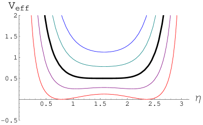
Figure 1: $V_{\rm eff}(\eta)$ versus $\eta$ for different values of $p_{\beta}$. The dark curve has $p_{\beta}=1$. The ones above it have $p_{\beta}>1$, and the ones below it have $0<p_{\beta}<1$.

A common feature, however, is that $\eta$ can never equal $0$ or $\pi$, so $\hat{\theta}^{5}=\sin\eta\neq 0$. This must be remedied by sending $\hat{\theta}^{A}\to O^{A}{}_{B}\hat{\theta}^{B}$ for some $SO(5)$ rotation, which we take to be of the form

$${O=\begin{pmatrix}\cos\gamma&0&0&0&-\sin\gamma\cr 0&1&0&0&0\cr 0&0&1&0&0\cr 0&0&0&1&0\cr\sin\gamma&0&0&0&\cos\gamma\end{pmatrix}\,.}$$

(7.68)

To focus the discussion, we restrict ourselves further to the simplest case where $\eta(t)=\eta_{0}$, a constant. In order to have $V_{\rm eff}^{\prime}(\eta)=0$, we must either set $\eta_{0}=\pi/2$ or, for $0<p_{\beta}<1$, choose $\sin^{2}\eta_{0}=p_{\beta}$. The latter choice is the one that we will treat here. Then one straightforwardly obtains

$${X^{\mu}}$$

The topology is a strip with boundaries at $\varphi=\pm\pi/2$ ending on the helices

$${X^{\mu}=\sin\gamma\,\left(0,(1-p_{\beta})t,\pm\sqrt{p_{\beta}(1-p_{\beta})}\sin t,\mp\sqrt{p_{\beta}(1-p_{\beta})}\cos t\right)\,.}$$

(7.70)

A double-helix Wilson loop also appears in [23].

7.2 The second ansatz

Now let us consider another obvious ansatz involving an abelian isometry:

$${\hat{\theta}^{1}+i\hat{\theta}^{2}}$$      

     

where $b$ is an arbitrary real number greater than $1$. Unless $b$ is rational, $\varphi$ is not a periodic coordinate. Nevertheless, correct equations of motion can be extracted from a reduced action,

$${S_{\rm reduced}=\int dt\,L\,,\qquad L={1\over 2}\left[\dot{\eta}^{2}+\cos^{2}\eta\,\dot{\xi}^{2}+\cos^{2}\eta(\cos^{2}\xi+b^{2}\sin^{2}\xi)\right]\,.}$$

(7.72)

This system is integrable [23, 24], with conserved quantities $I_{1}$, $I_{2}$, and $I_{3}$ defined by

$${I_{i}=\rho_{i}^{2}-\sum_{j\neq i}{(\rho_{i}\dot{\rho}_{j}-\rho_{j}\dot{\rho}_{i})^{2}\over m_{i}^{2}-m_{j}^{2}}\qquad m_{1}=1\,,\quad m_{2}=b\,,\quad m_{3}=0\,,}$$

(7.73)

and subject to $I_{1}+I_{2}+I_{3}=1$. The total energy may be expressed as $H=-(I_{1}+b^{2}I_{2})/2$. Because of these two linear relations, the two independent conserved quantities can be chosen as $I_{1}$, $I_{2}$, or as $H$, $I_{3}$.

To integrate the system explicitly, it is helpful to use elliptical coordinates $\zeta_{1}$, $\zeta_{2}$, defined equivalently as the solutions of

$${{\rho_{1}^{2}\over\zeta-1}+{\rho_{2}^{2}\over\zeta-b^{2}}+{\rho_{3}^{2}\over\zeta}=0\,,}$$

(7.74)

or through

$${\sin\eta={\sqrt{\zeta_{1}\zeta_{2}}\over b}\qquad\tan\xi={1\over b}\sqrt{-{(b^{2}-\zeta_{1})(b^{2}-\zeta_{2})\over(1-\zeta_{1})(1-\zeta_{2})}}\,,}$$

(7.75)

and subject to the inequalities

$${0\leq\zeta_{1}\leq 1\leq\zeta_{2}\leq b^{2}\,.}$$

(7.76)

It is straightforward to show that

$${\dot{\zeta}_{1}^{2}}$$

Note that $f(\zeta_{1})$ and $f(\zeta_{2})$ must be nonnegative on the range of values of $\zeta_{1}$, $\zeta_{2}$ that occur in a given solution. This puts constraints on the values of $\zeta_{a}$ and $\zeta_{b}$. Assuming that no $SO(5)$ rotation is applied, the boundary of the Wilson loop is at $\zeta_{1}=0$. Therefore $f(\zeta_{1})\geq 0$ for some closed interval whose left endpoint is $\zeta_{1}=0$. The right endpoint must be where $f(\zeta_{1})$ has a zero, namely at $1$ or $\zeta_{a}$, whichever is smallest. Similar considerations of the possible range of $\zeta_{2}$ leads to the following possibilities for solutions:

$${0}$$

The orbits of $\zeta_{1}$, $\zeta_{2}$ satisfy the integral equations

$${\int{d\zeta_{1}\over\sqrt{f(\zeta_{1})}}=\int{d\zeta_{2}\over\sqrt{f(\zeta_{2})}}\,.}$$

(7.79)

The explicit results (7.77) and (7.79) are not necessary to understand the qualitative features of supersymmetric Wilson loops associated with the ansatz (7.71). Consider a solution $\eta(t)$, $\xi(t)$ of the equations of motion following from (7.72), with $\eta(t)>0$ on some finite or semi-finite interval. Following the procedure outlined at the beginning of section 7, one obtains the following surface in $AdS_{5}\times S^{5}$:

$${X^{\mu}}$$

The real space part of the Wilson loop is

$${X^{\mu}=\dot{\eta}\,\left(\sin\varphi\cos\xi,-\cos\varphi\cos\xi,{1\over b}\sin b\varphi\sin\xi,-{1\over b}\cos b\varphi\sin\xi\right)\,,}$$

(7.81)

where now all quantities are evaluated at the time(s) when $\eta=0$.

It is worth noting an analogy with Poincaré’s stroboscopic map. In Poincaré’s setup, one starts with a system with two degrees of freedom (such as $\eta$ and $\xi$), selects one as the “timing” variable ($\eta$, let’s say), and then considers a map from the surface in phase space (the stroboscopic plane) defined by $\eta=0$, $\dot{\eta}>0$, and $H=E$, where $E$ is constant. The stroboscopic map is a volume-preserving bijection of the stroboscopic plane to itself defined by starting the system at a point on the stroboscopic plane, then evolving the system forward in time until it again meets the stroboscopic plane.

In the Wilson loop setup, $\eta=0$ is privileged once we choose $Z=c\hat{\theta}^{5}$. (But, as we remarked above, other choices can be made through $SO(5)$ rotations.) Energy conservation is also part of the Wilson loop setup. But instead of a single stroboscopic plane, we should now consider two disjoint planes: $P_{+}$ defined by $\dot{\eta}>0$ and $P_{-}$ defined by $\dot{\eta}<0$ (with $\eta=0$ and $H=E$ in both cases). There is then a natural map from $P_{+}$ to $P_{-}$ defined by taking a point on $P_{+}$ and evolving the system forward until it meets $P_{-}$. This is “half” of the stroboscopic map: to complete it one would evolve forward from $P_{-}$ back to $P_{+}$. A point on $P_{+}$ corresponds to one boundary of a Wilson loop correlator: (7.81) with $\dot{\eta}>0$. Such a curve can be fully specified by the data that selects a point on $P_{+}$: one can for example choose $\xi$, $\dot{\xi}$, and the total energy $E$ and solve for $\dot{\eta}>0$. Likewise a point on $P_{-}$ corresponds to a Wilson loop of the form (7.81) with $\dot{\eta}<0$.

The evolution of the dynamical system from $P_{+}$ to $P_{-}$ traces out the string worldsheet in $AdS_{5}\times S^{5}$. Because the boundary has two disjoint parts, the configuration represents the correlator of two Wilson loops. As in the example of the simple pendulum in section 7.1, it is also possible to have separatrix behavior, where for a particular choice of energy the system starts on $P_{+}$ and then evolves to infinite time without ever intersecting $P_{-}$. This corresponds to a single Wilson loop rather than a correlator of two.

A more explicit description of single Wilson loop cases can be obtained using the integrable structure and the elliptic coordinates $\zeta_{1}$ and $\zeta_{2}$. Recall that the boundary of the Wilson loop is at $\zeta_{1}=0$. For the system to evolve to infinite time without coming back to $\zeta_{1}=0$, it must asymptote to some other value, call it $\zeta_{*}$. There must be a double zero of $f(\zeta)$ at $\zeta=\zeta_{*}$, because otherwise the system reaches $\zeta_{1}=\zeta_{*}$ in finite time. The only possibility is $\zeta_{*}=\zeta_{a}=1$. There must also be an asymptotic value for $\zeta_{2}$, and there are two ways to arrange this. One way is to choose $\zeta_{b}=b^{2}$, so that there is a double root at $\zeta=b^{2}$ as well as at $\zeta=1$. Then, arranging signs so that $\dot{\zeta}_{2}>0$, one obtains a one-parameter family of smooth single-boundary surfaces by choosing an arbitrary boundary value of $\zeta_{2}\in(1,b^{2})$. The second way to get an asymptotic value for $\zeta_{2}$ at late time is to make $\zeta_{2}$ constant for all time: choose $\zeta_{2}=\zeta_{b}\in(1,b^{2})$.

A Wilson loop with the coincident boundaries similar to what was found in section 7.1 may be constructed by setting a double zero $\zeta_{a}=\zeta_{b}$ with $\zeta_{2}=\zeta_{a}$ for all time. Then $\zeta_{1}$ varies from $0$ to $1$ and the location of the double zero $\zeta_{a}=\zeta_{b}$ is a parameter of the solution. Alternatively, if $\zeta_{2}=\zeta_{b}=1$, then the location of $\zeta_{a}\in(0,1)$ is arbitrary and $\zeta_{1}$ varies from $0$ to $\zeta_{a}$. This latter solution corresponds to the physical pendulum $\eta(t)$ with $\xi=\pi/2$ and energy specified by $\zeta_{a}$.

7.3 Coincident boundaries

Figure 2: In (a) we see two coincident straight Wilson lines. We have separated them to ease visualization, but they are on top of each other. In (b) we plot two of the directions transverse to the D-brane and we see a string ending on the D-brane (represented by a cross) and a string leaving the D-brane. In (c) the two strings from (b) combine and move in a direction transverse to the D-brane. In (c) we see two coincident and oppositely oriented circular Wilson loops. Again we have separated them just to ease visualization.

A new feature of the annulus solutions discussed in section 7.1 and in the last paragraph of section 7.2 is that two boundaries are coincident but with opposite orientations. To simplify the discussion of this situation, let us first suppose that we have a straight Wilson loop and we now place an oppositely oriented Wilson line on top of the first, see figure 2(a). (This situation is in fact the $E\to\infty$ limit of the annular solution discussed in section 7.1). The second Wilson line has the opposite orientation, but it also has the opposite scalar charge, so it preserves the same supersymmetry. In this case, the corresponding surface in AdS has some zero modes. In other words, there is a family of surfaces that obey the boundary conditions. Let us assume that the Wilson lines are along $X^{1}$ on the D3-brane worldvolume. So we can consider any surface that is extended along $X^{1}$ and $Y^{1}$ and sits at any point in $Y^{2},\cdots,Y^{6}$. Thus the space of zero modes is non-compact. We see that such surfaces obey the equations (4.26), for a suitable choice of worldsheet coordinates. One way to understand the presence of these zero modes is to think of the strings ending on a D3 brane. We have a configuration with a string ending on the brane and one moving out of the D3-brane, figure 2(b). These two strings can be joined and moved out of the D3 brane, see figure 2(c).

Connected correlation functions of chiral Wilson loops vanish, via the following standard argument. Supersymmetry implies that the correlation function is independent of the separation. Together with clustering, this property gives a vanishing connected correlator. From the AdS point of view, the vanishing of the connected correlation function suggests that the pseudo-holomorphic annulus should have a fermionic zero-mode. As a point of comparison, recall that the pseudo-holomorphic disk is not generically invariant under R-symmetries respected by the boundary; for chiral Wilson loops in ${\bf R}^{2}$, the broken R-symmetries give rise to bosonic zero modes. All supersymmetries of the chiral Wilson loop should be respected by the disk in order to get expectation value $1$ rather than $0$. A counting of zero modes for the pseudo-holomorphic disk and annulus, lacking at present, is required to give a complete check of the non-renormalization and factorization of chiral Wilson loops in the AdS description. For the disk we expect three bosonic zero modes and no fermionic zero modes, while for the annulus, we expect at least one fermionic zero mode. Notice that for the straight Wilson loop in figure 2(a) we have fermion zero modes which are the fermionic partners of the bosonic zero modes for the supersymmetric quantum mechanics along the Wilson line. Similar considerations should apply to the closed Wilson loop correlators discussed in section 7.2, which may or may not have coincident boundaries, but clearly have zero regulated area as calculated from the $AdS_{5}\times S^{5}$ side of the duality.

8 Acknowledgements

We wish to thank A. Kapustin, E. Witten and K. Zarembo for useful discussions. Z. G. thanks the Institute for Advanced Study and the Boston University visitor program for hospitality during completion of this work. The research of A. D. is supported in part by grant RFBR 04-02-16538, grant for support of scientific schools NSh-8004.2006.2, and by the National Science Foundation Grant No. PHY-0243680. The research of S. G. is supported in part by the DOE under Grant No. DE-FG02-91ER40671, and by the Sloan Foundation. The work of J. M. was supported in part by DOE grant DE-FG01-91ER40654.

Appendix A The Wilson loop operator in the topologically
twisted theory

In this section we examine the properties of the Wilson loop operator from the point of view of the topologically twisted theory. For this purpose it is best to start with ten-dimensional super Yang Mills and latter reduce it to four dimensions. We consider the ten-dimensional theory on $\mathbb{C}^{5}$ and we consider the supersymmetry associated to the spinor that obeys $\Gamma_{MN}\epsilon=iJ_{MN}\epsilon$ in ten dimensions. Using this spinor we can transform the spinor index on the fermion into a vector index, as is usual in complex manifolds. In other words, we write the gaugino as $\chi=(\psi+\psi_{ij}\Gamma^{ij}+\psi_{\bar{i}}\Gamma^{\bar{i}}\Gamma^{12345})\epsilon$ where $\psi,~{}\psi_{ij},~{}\psi_{\bar{i}}$ are anticommuting, $\epsilon$ is a commuting spinor and $i,j=1,\cdots 5$.

Then the supersymmetry $Q$ associated to $\epsilon$ acts on the fields as

$$Q\psi = g^{i\bar{j}}{\cal F}_{i\bar{j}}$$ (A.82)

$$Q\psi_{ij} = {\cal F}_{ij}$$ (A.83)

$$Q\psi_{\bar{i}} = 0$$ (A.84)

$$Q{\cal A}_{i} = 0$$ (A.85)

$$Q{\cal A}_{\bar{i}} = \psi_{\bar{i}}\,.$$ (A.86)

We now consider Wilson loop operators which follow a holomorphic contour

$$W=\mathop{\rm tr}\nolimits Pe^{\int{\cal A}_{i}dz^{i}}\,,$$ (A.87)

where the contour has $\dot{z}^{\bar{i}}=0$. We see that (A.87) is annihilated by $Q$. On the other hand, if the contour $z^{i}(\tau)$ is topologically trivial, then we see that we can, at least formally, expand the operator (A.87) in terms of local operators which involve ${\cal F}_{ij}$ and holomorphic covariant derivatives ${\cal D}_{i}$. Such operators are all BRST trivial, since ${\cal F}_{ij}=Q\psi_{ij}$ and so are all their holomorphic covariant derivatives since ${\cal D}_{i}$ commutes with $Q$.

In order to go to the four-dimensional ${\cal N}=4$ super Yang Mills case, all we need to do is to dimensionally reduce by taking the four-dimensional spacetime to be spanned by the real part of the first four $z^{i}$ coordinates. We will then consider contours with $z^{5}=0$. The holomorphicity condition $d_{\tau}z^{\bar{i}}=0$ translates into the condition (2.4) relating the tangent vector to a point on $S^{4}\subset S^{5}$. The complex one-form in ten dimensions becomes ${\cal A}_{i}=A_{i}+i\Phi_{i}$, in terms of the four-dimensional gauge field and scalar.

Notice that this argument is very formal. In fact, it fails in the case of the topological string since in that case the circular Wilson loop has a nontrivial expectation value. We think that in four dimensions the result should hold. In fact, we can continuously deform the 1/16 BPS contour into the 1/4 BPS circular Wilson loop and then use the arguments in [8, 9].

Appendix B Wilson loops in the topological string

In this section we examine the question of the Wilson loop in the topological string context. We study the simplest case which arises when we consider branes on the deformed conifold and follow the large $N$ duality to the resolved conifold [18, 16, 17]

Let us start with the deformed conifold

$$XY-UV=\epsilon=\sum_{i=1}^{4}w_{i}^{2}$$ (B.88)

where we have set $X=w_{1}+iw_{2}$, $Y=w_{1}-iw_{2}$ , $U=w_{3}+iw_{4}$ , $V=-w_{3}+iw_{4}$. We have an $S^{3}$ when all $w_{i}$ are real. We can put three-dimensional branes on this $S^{3}$. We can now consider a string worldsheet that lies along the complex surface $U=V=0$. Such a surface obeys the complex equation $XY=\epsilon$. This is a noncompact surface which intersects the $S^{3}$ at $|Y|=\sqrt{|\epsilon|}$. We can consider the part of the original surface that lies along $|Y|\geq\sqrt{|\epsilon|}$. This is now a worldsheet that ends on an $S^{1}\subset S^{3}$. From the point of view of the Chern-Simons gauge theory on the $S^{3}$ this is a Wilson line in the fundamental representation. According to the Gopakumar-Vafa large $N$ transition [18], this will give rise to a closed string topological theory on the resolved conifold, which is specified by the equations

$$\left(\begin{array}[]{cc}X&U\\ V&Y\end{array}\right)\left(\begin{array}[]{c}\lambda_{1}\\ \lambda_{2}\end{array}\right)=0$$ (B.89)

where $(\lambda_{1},\lambda_{2})\in P^{1}$. There is nonzero solution only if $XY-UV=0$ and when $X=Y=U=V=0$ we have an additional solution. We are interested in the surface that is at $U=V=X=0$ and $Y$ non-zero. This implies that $\lambda_{2}=0$, so we are at a point on the $P^{1}$ as long as $Y\not=0$. This complex surface goes all the way to the origin. At this point it can wrap or not wrap the $P^{1}=S^{2}$ at the origin. So we see that we have at least two choices. One can see this very explicitly by looking at the metric for the resolved conifold [15]. In a patch where $\lambda_{1}\not=0$, we can choose complex coordinates $U,Y,\lambda={\lambda_{2}\over\lambda_{1}}$. Then the Kahler potential has the form

$$K=f(r^{2})+4a^{2}\log(1+|\lambda|^{2})~{},~{}~{}~{}~{}~{}~{}r^{2}\equiv(1+|\lambda|^{2})(|U|^{2}+|Y|^{2})\,,$$ (B.90)

where $a$ is the radius of the two-sphere at the origin. The simplest choice is for the surface to sit at $U=\lambda=0$. It is then spanned by the complex variable $Y$. This obviously obeys the right boundary conditions and it is a complex surface. In addition, its area is given by

$$A=\int{1\over 2}K_{Y\bar{Y}}dYd\bar{Y}={1\over 2}F^{\prime\prime}(r^{2})d(r^{2})d\varphi=\pi{dF\over dr^{2}}(r^{2}_{max})=\pi r_{max}^{4/3}-2\pi a^{2}\,.$$ (B.91)

Thus we see that after subtracting an $a$ independent constant the regularized area is

$${\rm Area}_{reg}=-2\pi a^{2}\,.$$ (B.92)

If we now consider the surface that in addition wraps the $S^{2}$, we get ${\rm Area}_{reg}=2\pi a^{2}$. These two possibilities give rise to the two terms in (4.40).

References

- [1] J. M. Maldacena, Phys. Rev. Lett. 80, 4859 (1998) [arXiv:hep-th/9803002].
- [2] S. J. Rey and J. T. Yee, Eur. Phys. J. C 22, 379 (2001) [arXiv:hep-th/9803001].
- [3] N. Drukker, D. J. Gross and H. Ooguri, Phys. Rev. D 60, 125006 (1999) [arXiv:hep-th/9904191].
- [4] N. Drukker and D. J. Gross, J. Math. Phys. 42, 2896 (2001) [arXiv:hep-th/0010274].
- [5] N. Drukker and B. Fiol, JHEP 0502, 010 (2005) [arXiv:hep-th/0501109]. S. Yamaguchi, arXiv:hep-th/0601089; hep-th/0603208. J. Gomis and F. Passerini, arXiv:hep-th/0604007.
- [6] K. Zarembo, Nucl. Phys. B 643, 157 (2002) [arXiv:hep-th/0205160].
- [7] C. Vafa, J. Math. Phys. 42, 2798 (2001) [arXiv:hep-th/0008142].
- [8] Z. Guralnik and B. Kulik, JHEP 0401, 065 (2004) [arXiv:hep-th/0309118].
- [9] Z. Guralnik, S. Kovacs and B. Kulik, arXiv:hep-th/0409091.
- [10] D. Joyce, arXiv:math.dg/0108088.
- [11] H. Lu, C. N. Pope and J. Rahmfeld, J. Math. Phys. 40, 4518 (1999) [arXiv:hep-th/9805151].
- [12] It is case in C. Vafa and E. Witten, Nucl. Phys. B 431, 3 (1994) [arXiv:hep-th/9408074], with a correction mentioned in page 16 of [13]
- [13] M. Bershadsky, C. Vafa and V. Sadov, Nucl. Phys. B 463, 420 (1996) [arXiv:hep-th/9511222].
- [14] M. Atiyah, J. M. Maldacena and C. Vafa, J. Math. Phys. 42, 3209 (2001) [arXiv:hep-th/0011256].
- [15] P. Candelas and X. C. de la Ossa, Nucl. Phys. B 342, 246 (1990).
- [16] H. Ooguri and C. Vafa, Nucl. Phys. B 577, 419 (2000) [arXiv:hep-th/9912123].
- [17] H. Ooguri and C. Vafa, Nucl. Phys. B 641 (2002) 3 [arXiv:hep-th/0205297].
- [18] R. Gopakumar and C. Vafa, Adv. Theor. Math. Phys. 3, 1415 (1999) [arXiv:hep-th/9811131].
- [19] E. Witten, Commun. Math. Phys. 121, 351 (1989).
- [20] H. Brezis and J. M. Coron, Comm. Math. Phys 92 (1983), 203-215.
- [21] V. Benci and J. M. Coron, Ann. Inst. Henri Poincar , Anal. Non Lin aire 2, 119-141 (1985). [ISSN 0294-1449]
- [22] H. Brezis, Bull. Am. Math. Soc 40 no.2 (2003), 179-201.
- [23] N. Drukker and B. Fiol, JHEP 0601, 056 (2006) [arXiv:hep-th/0506058].
- [24] G. Arutyunov, S. Frolov, J. Russo and A. A. Tseytlin, Nucl. Phys. B 671, 3 (2003) [arXiv:hep-th/0307191].
- [25] A. Neitzke and C. Vafa, arXiv:hep-th/0410178.
- [26] F. Canoura, J. D. Edelstein, L. A. P. Zayas, A. V. Ramallo and D. Vaman, arXiv:hep-th/0512087. J. F. G. Cascales and A. M. Uranga, JHEP 0411, 083 (2004) [arXiv:hep-th/0407132].
- [27] B. S. Acharya, J. P. Gauntlett and N. Kim, Phys. Rev. D 63, 106003 (2001) [arXiv:hep-th/0011190].
- [28] J. M. Maldacena and C. Nunez, Int. J. Mod. Phys. A 16, 822 (2001) [arXiv:hep-th/0007018].