Napoli DSF-T-31/2005

INFN-NA-31/2005

We propose a CFT description for a closed one-dimensional fully frustrated ladder of quantum Josephson junctions with Mobius boundary conditions [1]; we show how such a system can develop topological order thanks to flux fractionalization. Such a property is crucial for its implementation as a “protected” solid state qubit.

Keywords: Josephson Junction Ladder, Flux fractionalization, Topological order

PACS: 11.25.Hf, 74.50.+r, 03.75.Lm

Work supported in part by the European Communities Human Potential

Program under contract HPRN-CT-2000-00131 Quantum Spacetime

1 Introduction

Arrays of weakly coupled Josephson junctions provide an experimental realization of the two dimensional ($2D$) XY model physics. A Josephson junction ladder (JJL) is the simplest quasi-one dimensional version of an array in a magnetic field [2]; recently such a system has been the subject of many investigations because of its possibility to display different transitions as a function of the magnetic field, temperature, disorder, quantum fluctuations and dissipation. In this contribution we address the phenomenon of fractionalization of the flux quantum $\frac{hc}{2e}$ in a fully frustrated JJL, the basic question being how the phenomenon of Cooper pair condensation can cope with properties of charge (flux) fractionalization, typical of a low dimensional system with a discrete ($Z_{2}$ in our case) symmetry. Then we discuss how it is deeply related to the issue of topological order.

We must recall that charge fractionalization has been successfully hypothesized by R. Laughlin to describe the ground state of a strongly correlated $2D$ electron system, a quantum Hall fluid, at fractional fillings $\nu=\frac{1}{2p+1}$, $p=1,2,...$. In such a system charged excitations are present with fractional charge (anyons) and elementary flux $\frac{hc}{e}$. Furthermore the phenomenon of fractionalization of the elementary flux has been found more recently in the description of a quantum Hall fluid at non standard fillings $\nu=\frac{m}{mp+2}$ [3][4], within the context of $2D$ Conformal Field Theories (CFT) with a $Z_{m}$ twist.

In Refs. [5] it has been shown that the presence of a $Z_{2}$ symmetry accounts for more general boundary conditions for the propagating electron fields which arise in quantum Hall systems in the presence of impurities or defects. Furthermore such a symmetry is present also in the fully frustrated XY (FFXY) model or equivalently, see Ref. [6][1], in two dimensional Josephson junction arrays (JJA) with half flux quantum $\frac{1}{2}\frac{hc}{2e}$ threading each square cell and accounts for the degeneracy of the ground state.

It is interesting to notice that it is possible to generate non trivial topologies, i.e. the torus, in the context of a CFT approach. That allows in our case to show how non trivial global properties of the ground state wave function emerge and how closely they are related to the presence of half flux quanta, which can be viewed also as “topological defects”.

The concept of topological order was first introduced to describe the ground state of a quantum Hall fluid [7]. Although todays interest in topological order mainly derives from the quest for exotic non-Fermi liquid states relevant for high $T_{c}$ superconductors [8], such a concept is of much more general interest [9].

Two features of topological order are very striking: fractionally charged quasiparticles and a ground state degeneracy depending on the topology of the underlying manifold, which is lifted by quasiparticles tunnelling processes. For Laughlin fractional quantum Hall (FQH) states both these properties are well understood [10], but for superconducting devices the situation is less clear.

Josephson junctions networks appear to be good candidates for exhibiting topological order, as recently evidenced in Refs. [11][12] by means of Chern-Simons gauge field theory. Such a property may allow for their use as “protected” qubits for quantum computation.

The aim of this contribution is to show that the twisted model (TM) well adapts to describe the phenomenology of fully frustrated JJL with a topological defect and to analyze the implications of “closed” geometries on the ground state global properties. In particular we shall show that fully frustrated Josephson junction ladders (JJL) with non trivial geometry may support topological order, making use of conformal field theory techniques [1]. A simple experimental test of our predictions will be also proposed.

The paper is organized as follows.

In Section 2 we introduce the fully frustrated quantum Josephson junctions ladder (JJL) focusing on non trivial boundary conditions.

In Section 3 we recall some aspects of the $m$-reduction procedure [13], in particular we show how the $m=2$, $p=0$ case of our twisted model (TM) [3] well accounts for the symmetries of the model under study. In such a framework we give the whole primary fields content of the theory on the plane and exhibit the ground state wave function.

In Section 4 the symmetry properties of the ground state conformal blocks are analyzed and its relation with their topological properties shown.

In Section 5, starting from our CFT results, we show that the ground state is degenerate, the different states being accessible by adiabatic flux change techniques. Such a degeneracy is shown to be strictly related to the presence in the spectrum of quasiparticles with non abelian statistics and can be lifted non perturbatively through vortices tunneling.

In Section 6 some comments and outlooks are given.

In the Appendix we recall briefly the boundary states introduced in Ref. [5] in the framework of our TM.

2 Josephson junctions ladders with Mobius boundary conditions

In this Section we briefly describe the system we will study in the following, that is a closed ladder of Josephson junctions (see Fig.1) with Mobius boundary conditions. With each site $i$ we associate a phase $\varphi_{i}$ and a charge $2en_{i}$, representing a superconducting grain coupled to its neighbours by Josephson couplings; $n_{i}$ and $\varphi_{i}$ are conjugate variables satisfying the usual phase-number commutation relation. The system is described by the quantum phase model (QPM) Hamiltonian:

$$H=-\frac{E_{C}}{2}\sum_{i}\left(\frac{\partial}{\partial\varphi_{i}}\right)^{2}-\sum_{\left\langle ij\right\rangle}E_{ij}\cos\left(\varphi_{i}-\varphi_{j}-A_{ij}\right),$$ (1)

where $E_{C}=\frac{\left(2e\right)^{2}}{C}$ ($C$ being the grain capacitance) is the charging energy at site $i$, while the second term is the Josephson coupling energy between sites $i$ and $j$ and the sum is over nearest neighbours. $A_{ij}=\frac{2\pi}{\Phi_{0}}$ $\int_{i}^{j}A{\cdot}dl$ is the line integral of the vector potential associated to an external magnetic field $B$ and $\Phi_{0}=\frac{hc}{2e}$ is the superconducting flux quantum. The gauge invariant sum around a plaquette is $\sum_{p}A_{ij}=2\pi f$ with $f=\frac{\Phi}{\Phi_{0}}$, where $\Phi$ is the flux threading each plaquette of the ladder.

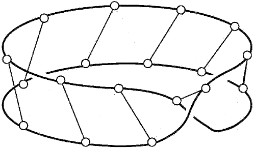
Figure 1: Josephson junction ladder with Mobius boundary conditions

Let us label the phase fields on the two legs with $\varphi_{i}^{\left(a\right)}$, $a=1,2$ and assume $E_{ij}=E_{x}$ for horizontal links and $E_{ij}=E_{y}$ for vertical ones. Let us also make the gauge choice $A_{ij}=+\pi f$ for the upper links, $A_{ij}=-\pi f$ for the lower ones and $A_{ij}=0$ for the vertical ones, which corresponds to a vector potential parallel to the ladder and taking opposite values on upper and lower branches.

Thus the effective quantum Hamiltonian (1) can be written as [2]:

$$-H = \frac{E_{C}}{2}\sum_{i}\left[\left(\frac{\partial}{\partial\varphi_{i}^{\left(1\right)}}\right)^{2}+\left(\frac{\partial}{\partial\varphi_{i}^{\left(2\right)}}\right)^{2}\right]+$$ (2)

$$\sum_{i}\left[E_{x}\sum_{a=1,2}\cos\left(\varphi_{i+1}^{\left(a\right)}-\varphi_{i}^{\left(a\right)}+\left(-1\right)^{a}\pi f\right)+E_{y}\cos\left(\varphi_{i}^{\left(1\right)}-\varphi_{i}^{\left(2\right)}\right)\right].$$

The correspondence between the effective quantum Hamiltonian (2) and our TM model can be best traced performing the change of variables [2]: $\varphi_{i}^{\left(1\right)}=X_{i}+\phi_{i}$, $\varphi_{i}^{\left(2\right)}=X_{i}-\phi_{i}$, so getting:

$$H = -\frac{E_{C}}{2}\sum_{i}\left[\left(\frac{\partial}{\partial X_{i}}\right)^{2}+\left(\frac{\partial}{\partial\phi_{i}}\right)^{2}\right]-$$ (3)

$$\sum_{i}\left[2E_{x}\cos\left(X_{i+1}-X_{i}\right)\cos\left(\phi_{i+1}-\phi_{i}-\pi f\right)+E_{y}\cos\left(2\phi_{i}\right)\right]$$

where $X_{i}$, $\phi_{i}$ (i.e. $\varphi_{i}^{\left(1\right)}$, $\varphi_{i}^{\left(2\right)}$) are only phase deviations of each order parameter from the commensurate phase and should not be identified with the phases of the superconducting grains [2].

When $f=\frac{1}{2}$ and $E_{C}=0$ (classical limit) the ground state of the $1D$ frustrated quantum XY (FQXY) model displays - in addition to the continuous $U(1)$ symmetry of the phase variables - a discrete $Z_{2}$ symmetry associated with an antiferromagnetic pattern of plaquette chiralities $\chi_{p}=\pm 1$, measuring the two opposite directions of the supercurrent circulating in each plaquette. The evidence for a chiral phase in Josephson junction ladders has been investigated in Ref. [14] while a field theoretical description of chiral order is developed in [15].

Performing the continuum limit of the Hamiltonian (3):

$$-H = \frac{E_{C}}{2}\int dx\left[\left(\frac{\partial}{\partial X}\right)^{2}+\left(\frac{\partial}{\partial\phi}\right)^{2}\right]+$$ (4)

$$\int dx\left[E_{x}\left(\frac{\partial X}{\partial x}\right)^{2}+E_{x}\left(\frac{\partial\phi}{\partial x}-\frac{\pi}{2}\right)^{2}+E_{y}\cos\left(2\phi\right)\right]$$

we see that the $X$ and $\phi$ fields are decoupled. In fact the $X$ term of the above Hamiltonian is that of a free quantum field theory while the $\phi$ one coincides with the quantum sine-Gordon model. Through an imaginary-time path-integral formulation of such a model [16] it can be shown that the $1D$ quantum problem maps into a $2D$ classical statistical mechanics system, the $2D$ fully frustrated XY model, where the parameter $\alpha=\left(\frac{E_{x}}{E_{C}}\right)^{\frac{1}{2}}$ plays the role of an inverse temperature [2]. For small $E_{C}$ there is a gap for creation of kinks in the antiferromagnetic pattern of $\chi_{p}$ and the ground state has quasi long range chiral order. We work in the regime ${E_{x}}\gg{E_{y}}$ where the ladder is well described by a CFT with central charge $c=2$.

We are now ready to introduce the modified ladder [1], see Fig. 1. In order to do so let us first require the $\varphi^{\left(a\right)}$, $a=1,2$, variables to recover the angular nature by compactification of both the up and down fields. In such a way the XY-vortices, causing the Kosterlitz-Thouless transition, are recovered. As a second step let us introduce at point $x=0$ a defect which couples the up and down edges through its interaction with the two legs, that is let us close the ladder and impose Mobius boundary conditions. In the limit of strong coupling such an interaction gives rise to non trivial boundary conditions for the fields [5]. In the following we give further details on such an issue, in particular we adopt the $m$-reduction technique [13][3], which accounts for non trivial boundary conditions [5] for the Josephson ladder in the presence of a defect line. In the Appendix the relevant chiral fields ${{\varphi}_{e}}^{\left(a\right)}$, $a=1,2$, which emerge from such conditions, are explicitly constructed, by using the folding procedure.

3 $m$-reduction technique

In this Section we focus on the $m$-reduction technique for the special $m=2$ case and apply it to the system described by the Hamiltonian (4). In the Appendix each phase field $\varphi^{\left(a\right)}$ is written as a sum of two fields of opposite chirality defined on an half-line, because of the presence of a defect at $x=0$. Within a ”bosonization” framework it is shown there how it is possible to reduce to a problem with two chiral fields $\varphi_{e}^{\left(a\right)}$, $a=1,2$, each defined on the whole $x-$axis, and the corresponding dual fields. Now we identify in the continuum such chiral phase fields $\varphi_{e}^{\left(a\right)}$, $a=1,2$, each defined on the corresponding leg, with the two chiral fields $Q^{\left(a\right)}$, $a=1,2$ of our CFT, the TM, with central charge $c=2$.

In order to construct such fields we start from a CFT with $c=1$ described in terms of a scalar chiral field $Q$ compactified on a circle with radius $R^{2}=2$, explicitly given by:

$$Q(z)=q-i\,p\,lnz+i\sum_{n\neq 0}\frac{a_{n}}{n}z^{-n}$$ (5)

with $a_{n}$, $q$ and $p$ satisfying the commutation relations $\left[a_{n},a_{n^{\prime}}\right]=n\delta_{n,n^{\prime}}$ and $\left[q,p\right]=i$; its primary fields are the vertex operators $U^{\alpha_{l}}\left(z\right)=:e^{i\alpha_{l}Q(z)}:$ and $\alpha_{l}=\frac{l}{\sqrt{2}},l=1,2$. It is possible to give a plasma description through the relation $\left|\psi\right|^{2}=e^{-\beta H_{eff}}$ where $\psi\left(z_{1},...,z_{N}\right)=\left\langle N\alpha|\prod_{i=1}^{N}U^{\alpha_{l}}(z_{i})|0\right\rangle=\prod_{i<j=1}^{N}\left(z_{i}-z_{j}\right)^{\frac{l^{2}}{2}}$ is the ground state wave function. It can be immediately seen that $H_{eff}=-l^{2}\sum_{i<j=1}^{N}\ln\left|z_{i}-z_{j}\right|$ and $\beta=\frac{2}{R^{2}}=1$, that is only vorticity $v=1,2$ vortices are present in the plasma.

Starting from such a CFT mother theory one can use the $m$-reduction procedure, which consists in considering the subalgebra generated only by the modes in eq. (5) which are a multiple of an integer $m$, so getting a $c=m$ orbifold CFT (daughter theory, i.e. the twisted model (TM)) [3]. With respect to the special $m=2$ case, the fields in the mother CFT can be organized into components which have well defined transformation properties under the discrete $Z_{2}$ (twist) group, which is a symmetry of the TM. By using the mapping $z\rightarrow z^{1/2}$ and by making the identifications $a_{2n+l}\longrightarrow\sqrt{2}a_{n+l/2}$, $q\longrightarrow\frac{1}{\sqrt{2}}q$ the $c=2$ daughter CFT is obtained. It is interesting to notice that such a daughter CFT gives rise to a vortices plasma of half integer vorticity, that is to a fully frustrated XY model, as it will appear in the following.

Its primary fields content can be expressed in terms of a $Z_{2}$-invariant scalar field $X(z)$, given by

$$X(z)=\frac{1}{2}\left(Q^{(1)}(z)+Q^{(2)}(z)\right),$$ (6)

describing the continuous phase sector of the new theory, and a twisted field

$$\phi(z)=\frac{1}{2}\left(Q^{(1)}(z)-Q^{(2)}(z)\right),$$ (7)

which satisfies the twisted boundary conditions $\phi(e^{i\pi}z)=-\phi(z)$ [3]. Such fields coincide with the ones introduced in eq. (4).

The whole TM theory decomposes into a tensor product of two CFTs, a twisted invariant one with $c=\frac{3}{2}$ and the remaining $c=\frac{1}{2}$ one realized by a Majorana fermion in the twisted sector. In the $c=\frac{3}{2}$ subtheory the primary fields are composite vertex operators $V\left(z\right)=U_{X}^{\alpha_{l}}\left(z\right)\psi\left(z\right)$ or $V_{qh}\left(z\right)=U_{X}^{\alpha_{l}}\left(z\right)\sigma\left(z\right)$, where $U_{X}^{\alpha_{l}}\left(z\right)=\frac{1}{\sqrt{z}}:e^{i\alpha_{l}X(z)}:$ is the vertex of the charged sector with $\alpha_{l}=\frac{l}{2},l=1,...,4$ for the $SU(2)$ Cooper pairing symmetry used here.

Regarding the other component, the highest weight state in the neutral sector can be classified by the two chiral operators:

$$\psi\left(z\right) = \frac{1}{2\sqrt{z}}\left(:e^{i\sqrt{2}\phi\left(z\right)}:+:e^{i\sqrt{2}\phi\left(-z\right)}:\right),~{}~{}~{}~{}~{}~{}$$

$$\overline{\psi}\left(z\right) = \frac{1}{2\sqrt{z}}\left(:e^{i\sqrt{2}\phi\left(z\right)}:-:e^{i\sqrt{2}\phi\left(-z\right)}:\right);$$ (8)

which correspond to two $c=\frac{1}{2}$ Majorana fermions with Ramond (invariant under the $Z_{2}$ twist) or Neveu-Schwartz ($Z_{2}$ twisted) boundary conditions [3] in a fermionized version of the theory. Let us point out that the energy-momentum tensor of the Ramond part of the neutral sector develops a cosine term:

$$T_{\psi}\left(z\right)=-\frac{1}{4}\left(\partial\phi\right)^{2}-\frac{1}{16z^{2}}\cos\left(2\sqrt{2}\phi\right),$$ (9)

a clear signature of a tunneling phenomenon which selects a new stable vacuum, the linear superposition of the two ground states. The Ramond fields are the degrees of freedom which survive after the tunneling and the $Z_{2}$ (orbifold) symmetry, which exchanges the two Ising fermions, is broken.

So the whole energy-momentum tensor within the $c=\frac{3}{2}$ subtheory is:

$$T=T_{X}\left(z\right)+T_{\psi}\left(z\right)=-\frac{1}{2}\left(\partial X\right)^{2}-\frac{1}{4}\left(\partial\phi\right)^{2}-\frac{1}{16z^{2}}\cos\left(2\sqrt{2}\phi\right).$$ (10)

The correspondence with the Hamiltonian in eq. (4) is more evident once we observe that the neutral current $\partial\phi$ appearing above coincides with the term $\partial\phi-\frac{\pi}{2}$ of eq. (4), since the $\frac{\pi}{2}$-term coming there from the frustration condition, here it appears in $\partial\phi$ as a zero mode, i.e. a classical mode. Besides the fields appearing in eq. (8) there are the $\sigma\left(z\right)$ fields, also called the twist fields, which appear in the primary fields $V_{qh}\left(z\right)$ combined to a vertex with charge $\frac{e}{4}$. The twist fields have non local properties and decide also for the non trivial properties of the vacuum state, which in fact can be twisted or not in our formalism. Such a property for the vacuum is more evident for the torus topology, where the $\sigma$-field is described by the conformal block $\chi_{\frac{1}{16}}$ (see Section 4).

The evidence of a phase transition in ladder systems at $c={\frac{3}{2}}$ has been investigated in [17] within a CFT framework. Within this framework the ground state wave function is described as a correlator of $N_{2e}$ Cooper pairs:

$$<N_{2e}\alpha|\prod_{i=1}^{N_{2e}}V^{\sqrt{2}}(z_{i})|0>=\prod_{i<i^{\prime}=1}^{N_{2e}}(z_{i}-z_{i^{\prime}})Pf\left(\frac{1}{z_{i}-z_{i^{\prime}}}\right)$$ (11)

where $Pf\left(\frac{1}{z_{i}-z_{i^{\prime}}}\right)=\mathcal{A}\left(\frac{1}{z_{1}-z_{2}}\frac{1}{z_{3}-z_{4}}\dots\right)$ is the antisymmetrized product over pairs of Cooper pairs, so reproducing well known results [18]. In a similar way we also are able to evaluate correlators of $N_{2e}$ Cooper pairs in the presence of (quasi-hole) excitations [18][3] with non Abelian statistics [19]. It is now interesting to notice that the charged contribution appearing in the correlator of $N_{e}$ electrons is just: $<N_{e}\alpha|\prod_{i=1}^{N_{2e}}U_{X}^{1/2}(z_{i})|0>=\prod_{i<i^{\prime}=1}^{N_{e}}(z_{i}-z_{i^{\prime}})^{1/4}$, giving rise to a vortices plasma with $H_{eff}=-\frac{1}{4}\sum_{i<j=1}^{N}\ln\left|z_{i}-z_{j}\right|$ at the corresponding ”temperature” $\beta=\frac{2}{R_{X}^{2}}=2$, that is it describes vortices with vorticity $v=\frac{1}{2}$!

On closed annulus geometries, as it is the discretized analogue of a torus, we must properly account for boundary conditions at the ends of the finite lattice since they determine in the continuum the pertinent conformal blocks yielding the statistics of quasiparticles as well as the ground state degeneracy. We have two possible boundary conditions which correspond to two different ways to close the double lattice, i.e. $\varphi_{N}^{\left(a\right)}\rightarrow\varphi_{1}^{\left(a\right)}$ or $\varphi_{N}^{\left(a+1\right)}\rightarrow\varphi_{1}^{\left(a\right)}$, $a=1,2$. It is not difficult to work out that, for the ladder case, the twisted boundary conditions can be implemented only on the odd lattice.

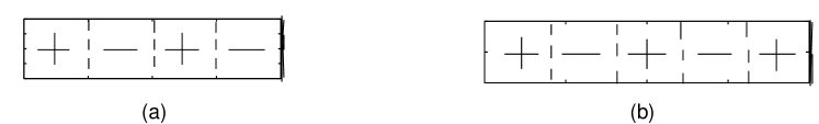
Figure 2: boundary conditions: (a) untwisted; (b) twisted.

Indeed for $f=\frac{1}{2}$ the ladder is invariant under the shift of two sites, so that there are two topologically inequivalent boundary conditions for even or odd number of sites. In the even case the end sites are of the same kind of the starting one, while in the odd case a ferromagnetic line corresponds to an antiferromagnetic one. The even (odd) case corresponds to untwisted (twisted) boundary conditions, as depicted in Fig. 2. The odd case selects out two degenerate ground states which belong to a non trivial topological sector, indeed the system may develop topological order in the twisted sector of our theory. Let us notice that in the discrete case not all the vacua in the different sectors of our theory are connected. For instance the states in the untwisted sector, which correspond to the even ladder, are physically disconnected from those of the twisted one, which correspond to the odd ladder.

4 Symmetry properties of the TM conformal blocks

In Section 3 we identified our chiral fields $Q^{(a)}$ with the continuum limit of the Josephson phase $\varphi^{\left(a\right)}$ defined on the two legs of the ladder respectively and considered non trivial boundary conditions at its ends, so constructing a version in the continuum of the discrete system. By using standard conformal field theory techniques it is now possible to generate the torus topology, starting from the edge theory, just defined in the previous Section. That is realized by evaluating the $N-$vertices correlator

$$\left\langle n\right|V_{\alpha}\left(z_{1}\right)...V_{\alpha}\left(z_{N}\right)e^{2\pi i\tau L_{0}}\left|n\right\rangle$$ (12)

where $V_{\alpha}\left(z_{i}\right)$ is the generic primary field of Section 3 representing the excitation at $z_{i}$, $L_{0}$ is the Virasoro generator for dilatations and $\tau$ the proper time. The neutrality condition $\sum\alpha=0$ must be satisfied and the sum over the complete set of states $\left|n\right\rangle$ is indicating that a trace must be taken. For the present paper it is not necessary to go through such a calculation but it is very illuminating for the non expert reader to pictorially represent the above operation in terms of an edge state (that is a primary state defined at a given $\tau$) which propagates interacting with external fields at $z_{1}...z_{N}$ and finally getting back to itself. In such a way a $2D$ surface is generated with the torus topology. From such a picture it is evident then how the degeneracy of the non perturbative ground state is closely related to the number of primary states. Furthermore, since in this paper we are interested in the understanding of the topological properties of the system, we can consider only the center of mass contribution in the above correlator, so neglecting its short distances properties. To such an extent the one-point functions are extensively reported in the following.

On the torus [4] the TM primary fields are described in terms of the conformal blocks of the $Z_{2}$-invariant $c=3/2$ subtheory and of the non invariant $c=1/2$ Ising model, so reflecting the decomposition on the plane outlined in the previous Section. The following characters

$$\bar{\chi}_{0}(w_{n}|\tau) =\frac{1}{2}\left(\sqrt{\frac{\theta_{3}(w_{n}|\tau)}{\eta(\tau)}}+\sqrt{\frac{\theta_{4}(w_{n}|\tau)}{\eta(\tau)}}\right)$$

$$\bar{\chi}_{\frac{1}{2}}(w_{n}|\tau) =\frac{1}{2}\left(\sqrt{\frac{\theta_{3}(w_{n}|\tau)}{\eta(\tau)}}-\sqrt{\frac{\theta_{4}(w_{n}|\tau)}{\eta(\tau)}}\right)$$

$$\bar{\chi}_{\frac{1}{16}}(w_{n}|\tau) =\sqrt{\frac{\theta_{2}(w_{n}|\tau)}{2\eta(\tau)}}$$

express the primary fields content of the Ising model with Neveu-Schwartz ($Z_{2}$ twisted) boundary conditions, while

$$\chi_{(0)}^{c=3/2}(w_{n}|w_{c}|\tau) = \chi_{0}(w_{n}|\tau)K_{0}(w_{c}|\tau)+\chi_{\frac{1}{2}}(w_{n}|\tau)K_{2}(w_{c}|\tau)$$ (13)

$$\chi_{(1)}^{c=3/2}(w_{n}|w_{c}|\tau) = \chi_{\frac{1}{16}}(w_{n}|\tau)\left(K_{1}(w_{c}|\tau)+K_{3}(w_{c}|\tau)\right)$$ (14)

$$\chi_{(2)}^{c=3/2}(w_{n}|w_{c}|\tau) = \chi_{\frac{1}{2}}(w_{n}|\tau)K_{0}(w_{c}|\tau)+\chi_{0}(w_{n}|\tau)K_{2}(w_{c}|\tau)$$ (15)

represent those of the $Z_{2}$-invariant $c=3/2$  CFT. They are given in terms of a “charged” $K_{\alpha}(w_{c}|\tau)$ contribution, (see definition given below) and a “neutral” one $\chi_{\beta}(w_{n}|\tau)$, (the conformal blocks of the Ising Model), where $w_{c}=\frac{1}{2\pi i}\ln z_{c}$ and $w_{n}=\frac{1}{2\pi i}\ln z_{n}$ are the torus variables of “charged” and “neutral” components respectively.

In order to understand the physical significance of the $c=2$ conformal blocks in terms of the charged low energy excitations of the system, let us evidence their electric charge (magnetic flux contents in the dual theory, which is obtained by exchanging the compactification radius $R_{e}^{2}\rightarrow R_{m}^{2}$ in the charged sector of the CFT). In order to do so let us consider the “charged” sector conformal blocks appearing in eqs. (13-15):

$$K_{2l+i}(w|\tau)=\frac{1}{\eta\left(\tau\right)}\Theta\left[\begin{array}[]{c}\frac{2l+i}{4}\\ 0\end{array}\right](2w|4\tau),~{}~{}~{}~{}~{}\forall\left(l,i\right)\in\left(0,1\right)^{2}.$$ (16)

They correspond to primary fields with conformal dimensions $h_{2l+i}=\frac{1}{2}\alpha_{\left(l,i\right)}^{2}=\frac{1}{2}\left(\frac{2l+i}{2}+2\delta_{\left(l+i\right),0}\right)^{2}$ and electric charges $2e\left(\frac{\alpha_{\left(l,i\right)}}{R_{X}}\right)$(magnetic charges in the dual theory $\frac{hc}{2e}\left(\alpha_{\left(l,i\right)}R_{X}\right)$), $R_{X}=1$ being the compactification radius. More explicitly the electric charges (magnetic charges in the dual theory) are the following:

$$\begin{array}[]{cccc}l=0&i=0&q_{e}=4e&\left(q_{m}=2\frac{hc}{2e}\right)\\ l=1&i=0&q_{e}=2e&\left(q_{m}=\frac{hc}{2e}\right)\\ l=0&i=1&q_{e}=e&\left(q_{m}=\frac{1}{2}\frac{hc}{2e}\right)\\ l=1&i=1&q_{e}=3e&\left(q_{m}=\frac{3}{2}\frac{hc}{2e}\right)\end{array}.$$ (17)

If we now turn to the whole $c=2$ theory, the characters of the twisted sector are given by:

$$\chi_{(0)}^{+}(w_{n}|w_{c}|\tau) = \bar{\chi}_{\frac{1}{16}}(w_{n}|\tau)\left(\chi_{0}^{c=3/2}(w_{n}|w_{c}|\tau)+\chi_{2}^{c=3/2}(w_{n}|w_{c}|\tau)\right)$$

$$= \bar{\chi}_{\frac{1}{16}}\left(\chi_{0}+\chi_{\frac{1}{2}}\right)\left(K_{0}+K_{2}\right)$$

$$\chi_{(1)}^{+}(w_{n}|w_{c}|\tau) = \left(\bar{\chi}_{0}(w_{n}|\tau)+\bar{\chi}_{\frac{1}{2}}(w_{n}|\tau)\right)\chi_{1}^{c=3/2}(w_{n}|w_{c}|\tau)$$

$$= \chi_{\frac{1}{16}}\left(\bar{\chi}_{0}+\bar{\chi}_{\frac{1}{2}}\right)\left(K_{1}+K_{3}\right)$$

$$\chi_{(0)}^{-}(w_{n}|w_{c}|\tau) = \bar{\chi}_{\frac{1}{16}}(w_{n}|\tau)\left(\chi_{0}^{c=3/2}(w_{n}|w_{c}|\tau)-\chi_{2}^{c=3/2}(w_{n}|w_{c}|\tau)\right)$$

$$= \bar{\chi}_{\frac{1}{16}}\left(\chi_{0}-\chi_{\frac{1}{2}}\right)\left(K_{0}-K_{2}\right)$$

$$\chi_{(1)}^{-}(w_{N}|w_{c}|\tau) = \left(\bar{\chi}_{0}(w_{n}|\tau)-\bar{\chi}_{\frac{1}{2}}(w_{n}|\tau)\right)\chi_{1}^{c=3/2}(w_{n}|w_{c}|\tau)$$

$$= \chi_{\frac{1}{16}}\left(\bar{\chi}_{0}-\bar{\chi}_{\frac{1}{2}}\right)\left(K_{1}+K_{3}\right).$$

Furthermore the characters of the untwisted sector are [4]:

$$\tilde{\chi}_{(0)}^{+}(w_{n}|w_{c}|\tau) =\bar{\chi}_{0}(w_{n}|\tau)\chi_{(0)}^{c=3/2}(w_{n}|w_{c}|\tau)+\bar{\chi}_{\frac{1}{2}}(w_{n}|\tau)\chi_{(2)}^{c=3/2}(w_{n}|w_{c}|\tau)$$ (22)

$$=\left(\bar{\chi}_{0}\chi_{0}+\bar{\chi}_{\frac{1}{2}}\chi_{\frac{1}{2}}\right)K_{0}+\left(\bar{\chi}_{0}\chi_{\frac{1}{2}}+\bar{\chi}_{\frac{1}{2}}\chi_{0}\right)K_{2}$$

$$\tilde{\chi}_{(1)}^{+}(w_{n}|w_{c}|\tau) =\bar{\chi}_{0}(w_{n}|\tau)\chi_{(2)}^{c=3/2}(w_{n}|w_{c}|\tau)+\bar{\chi}_{\frac{1}{2}}(w_{n}|\tau)\chi_{(0)}^{c=3/2}(w_{n}|w_{c}|\tau)$$ (23)

$$=\left(\bar{\chi}_{0}\chi_{\frac{1}{2}}+\bar{\chi}_{\frac{1}{2}}\chi_{0}\right)K_{0}+\left(\bar{\chi}_{0}\chi_{0}+\bar{\chi}_{\frac{1}{2}}\chi_{\frac{1}{2}}\right)K_{2}$$

$$\tilde{\chi}_{(0)}^{-}(w_{n}|w_{c}|\tau) =\bar{\chi}_{0}(w_{n}|\tau)\chi_{(0)}^{c=3/2}(w_{n}|w_{c}|\tau)-\bar{\chi}_{\frac{1}{2}}(w_{n}|\tau)\chi_{(2)}^{c=3/2}(w_{n}|w_{c}|\tau)$$ (24)

$$=\left(\bar{\chi}_{0}\chi_{0}-\bar{\chi}_{\frac{1}{2}}\chi_{\frac{1}{2}}\right)K_{0}+\left(\bar{\chi}_{0}\chi_{\frac{1}{2}}-\bar{\chi}_{\frac{1}{2}}\chi_{0}\right)K_{2}$$

$$\tilde{\chi}_{(1)}^{-}(w_{n}|w_{c}|\tau) =\bar{\chi}_{0}(w_{n}|\tau)\chi_{(2)}^{c=3/2}(w_{n}|w_{c}|\tau)-\bar{\chi}_{\frac{1}{2}}(w_{n}|\tau)\chi_{(0)}^{c=3/2}(w_{n}|w_{c}|\tau)$$ (25)

$$=\left(\bar{\chi}_{0}\chi_{\frac{1}{2}}-\bar{\chi}_{\frac{1}{2}}\chi_{0}\right)K_{0}+\left(\bar{\chi}_{0}\chi_{0}-\bar{\chi}_{\frac{1}{2}}\chi_{\frac{1}{2}}\right)K_{2}$$

$$\tilde{\chi}_{(0)}(w_{n}|w_{c}|\tau) =\bar{\chi}_{\frac{1}{16}}(w_{n}|\tau)\chi_{(1)}^{c=3/2}(w_{n}|w_{c}|\tau)=\bar{\chi}_{\frac{1}{16}}\chi_{\frac{1}{16}}\left(K_{1}+K_{3}\right).$$ (26)

Such a factorization is a consequence of the parity selection rule ($m$-ality), which gives a gluing condition for the “charged” and “neutral” excitations. The conformal blocks given above represent the collective states of highly correlated vortices, which appear to be incompressible. In order to show the corresponding symmetry properties it is useful to give a pictorial description of the conformal blocks appearing in eq. (16). To such an extent let us imagine to cut the torus along the $A$-cycle. The different primary fields then can be seen as excitations which propagate along the $B$-cycle and interact with the external Cooper pair at point $w=\frac{1}{2\pi i}\ln z$. We can now test the symmetry properties of the characters of the theory (given above) by simply evaluating the Bohm-Aharonov phase they pick up while a Cooper pair is taken along the closed $A$-cycle. In order to do that, it is important to notice that the transport of the ”Cooper pair” from the upper (with isospin up) leg to the down (with isospin down) leg can be realized by a translation of the variables $w_{c}$ and $w_{n}$, which must be identical for the ”charged” and the ”neutral” sectors. So, under a $2\pi$-rotation the torus variables transforms as $\Delta w_{c}=\Delta w_{n}=1$. It is easy to check that:

$$K_{0,2}(w_{c}+1|\tau)=K_{0,2}(w_{c}|\tau),~{}~{}K_{1,3}(w_{c}+1|\tau)=-K_{1,3}(w_{c}|\tau).$$ (27)

The change in sign given in eq. (27) under a $2\pi$-rotation is strictly related to the presence in the spectrum of excitations carrying fractionalized charge quanta. Now, turning on also the neutral sector contribution in the Cooper pair transport along the $A$-cycle we obtain in a straightforward way:

$$\chi_{0,\frac{1}{2}}(w_{n}+1|\tau)=\chi_{0,\frac{1}{2}}(w_{n}|\tau),~{}~{}\chi_{\frac{1}{16}}(w_{n}+1|\tau)=i\chi_{\frac{1}{16}}(w_{n}|\tau)$$ (28)

the same is true for the characters $\bar{\chi}_{\beta}$. A phase $i=e^{i\frac{\pi}{2}}$ appears in the $\chi_{\frac{1}{16}}$ character due to the presence of a half-flux.

As a result the ground state described by eq. (26):

$$\tilde{\chi}_{(0)}(w_{n}|w_{c}|\tau)=\bar{\chi}_{\frac{1}{16}}\chi_{\frac{1}{16}}\left(K_{1}+K_{3}\right)$$ (29)

does not change sign under, $\Delta w_{c}=\Delta w_{n}=1$, the transport of a Cooper pair along the closed $A$-cycle. In fact the negative sign coming from the continuous phase sector being compensated by the negative sign coming from the other sector! Of course the same is true for all the other characters of the untwisted sector, i.e. we cannot trap a half flux quantum in the hole in the untwisted sector.

Instead in the twisted sector the ground state wave-functions show a non trivial behavior. In fact under $\Delta w_{c}=\Delta w_{n}=1$

$$\chi_{\left(0\right)}^{\pm}(w_{n}+1|w_{c}+1|\tau)=+i\chi_{\left(0\right)}^{\pm}(w_{n}|w_{c}|\tau),~{}~{}\chi_{\left(1\right)}^{\pm}(w_{n}+1|w_{c}+1|\tau)=-i\chi_{\left(1\right)}^{\pm}(w_{n}|w_{c}|\tau),$$ (30)

The change in phase given above evidences the presence of a half flux quantum in the hole. In fact in the twisted case geometry (see Fig2) the Cooper pair flows along the ladder and changes isospin in a $2\pi$-period, so implying that in such a case the transport of a Cooper pair from a given point $w$ on the $A$-cycle to the same point has a $4\pi$-period, that is it corresponds to $\Delta w_{c}=\Delta w_{n}=2$. Under this transformation the characters get the following non trivial phase:

$$\chi_{\left(0,1\right)}^{\pm}(w_{n}+2|w_{c}+2|\tau)=-\chi_{\left(0,1\right)}^{\pm}(w_{n}|w_{c}|\tau),$$ (31)

so explicitly evidencing the trapping of $\frac{1}{2}\frac{hc}{2e}$ in the hole.

It is worthwhile to notice that the properties just discussed are independent of the short distance properties of the vortices plasma, the only crucial requirement for its stability being the neutrality condition.

5 Topological order and “protected” qubits

The aim of this Section is to fully exploit the issue of topological order in a quantum JJL. In order to meet such a request let us use the results of the $2$-reduction technique for the torus topology [4]. For closed geometries the JJL with Mobius boundary conditions gives rise to a line defect in the bulk. So it becomes mandatory to use a folding procedure to map the problem with a defect line into a boundary one, where the defect line appears as a boundary state. The TM boundary states have been constructed in Ref. [5] together with the corresponding chiral partition functions and briefly recalled in the Appendix. In particular we get an ”untwisted” sector and a ”twisted” one, corresponding to periodic and Mobius boundary conditions respectively. That gives rise to an essential difference in the low energy spectrum for the system under study: in the first case only two-spinon excitations are possible (i.e. ${SU(2)}_{2}$ integer spin representations) while, in the last case, the presence of a topological defect provides a clear evidence of single-spinon excitations (i.e. ${SU(2)}_{2}$ half-integer spin representations). All that takes place in close analogy with spin-1/2 closed zigzag ladders, which are expected to map to fully frustrated Josephson ladders in the extremely quantum limit. In this way all previous results obtained by means of exact diagonalization techniques [20] are recovered.

In the following we discuss topological order referring to the characters which in turn are related to the different boundary states present in the system through such chiral partition functions [1]. We can build a topological invariant $\mathcal{P}=\prod\limits_{\gamma}\chi_{p}$ where $\gamma$ is a closed contour that goes around the hole. Such a choice allows us to define two degenerate ground states with $\mathcal{P}=1$ and $\mathcal{P}=-1$ respectively, labelled $\left|0\right\rangle,\left|1\right\rangle$, as in Fig. 3(a): there must be an odd number of plaquettes (odd ladder) to satisfy this condition which is imposed by the request of topological protection. The value $\mathcal{P}=-1$ selects twisted boundary conditions at the ends of the chain while $\mathcal{P}=1$ selects periodic boundary conditions (see Fig. 3(b)). The case of finite discrete systems has been discussed in detail in Ref. [21], our theory is its counterpart in the continuum.

Figure 3: degenerate ground states for: (a) odd ladder, $\mathcal{P}=\pm 1$; (b) even ladder, $\mathcal{P}=1$.

In fact it is now possible to identify the two degenerate ground states shown in Fig.3(a) with the twisted characters (4-4):

$$\left|0\right\rangle\rightarrow\chi_{\left(0\right)}^{+}(w_{c}|\tau),~{}~{}\left|1\right\rangle\rightarrow\chi_{\left(1\right)}^{+}(w_{c}|\tau),$$ (32)

where it is meant that $w_{n}$ is fixed to zero (see also (55) and (56) of Appendix), then it is possible to remove such a degeneracy through vortices tunneling. The last operation is also needed in order to prepare the qubit in a definite state.

In fact such two states can be distinguished from all the other ones. First of all, being in the twisted sector they trap a half flux quantum inside the central hole (see (31)). The trapped half flux quantum can be experimentally detected, so giving a way to read out the twisted states of the system.

Now, upon performing an adiabatic change of local magnetic fields which drags one half vortex across the system, i.e. through the transport of a half flux quantum around the $B$-cycle of the torus, we are able to fully distinguish such two states with respect to the other pair of states, $\chi_{\left(0\right)}^{-}$ and $\chi_{\left(1\right)}^{-}$, of the twisted sector.

In fact, the transformations

$$\chi_{(0)}^{+}(\tau/2|w_{C}+\tau/2|\tau) = -ie^{-i\pi w_{C}}q^{-3/8}\chi_{(1)}^{+}(w_{C}|\tau)$$ (33)

$$\chi_{(1)}^{+}(\tau/2|w_{C}+\tau/2|\tau) = ie^{-i\pi w_{C}}q^{-5/8}\chi_{(0)}^{+}(w_{C}|\tau),$$ (34)

$$\chi_{(0)}^{-}(\tau/2|w_{C}+\tau/2|\tau) = 0$$ (35)

$$\chi_{(1)}^{-}(\tau/2|w_{C}+\tau/2|\tau) = 0$$ (36)

just imply a flip among the two ground states of the system

$$\left|0\right\rangle\rightarrow\left|1\right\rangle~{}\text{and}~{}\left|1\right\rangle\rightarrow\left|0\right\rangle,$$ (37)

while the other two twisted states are annihilated.

Finally it should be noticed that the presence of the twist operators $\sigma$, described here by the Ising character $\chi_{\frac{1}{16}}$, gives rise to non Abelian statistics, which can be evidenced by their fusion rules $\sigma\sigma=\mathbf{1}+\psi$ [18][4].

6 Brief summary with comments

In this contribution we presented a simple collective description of a ladder of Josephson junctions with a macroscopic half flux quanta trapped in the hole of a ladder. It was shown how the phenomenon of flux fractionalization takes place within the context of a $2D$ conformal field theory with a $Z_{2}$ twist, the TM. The presence of a $Z_{2}$ symmetry indeed accounts for more general boundary conditions for the fields describing the Cooper pairs propagating on the ladder legs, which arise from the presence of a magnetic impurity strongly coupled with the Josephson phases. It should be noticed that it would be useful to extend our approach to a generic frustration $f=\frac{1}{m}$. For closed geometries and in the limit of the continuum the phase fields $\varphi^{(a)}$ defined on the two legs were identified with the two chiral Fubini fields $Q^{(a)}$ of our TM, and a correspondence between the energy momentum density tensor for such fields (or better the $X$ and $\phi$ fields of eqs. (6)-(7)) and the Hamiltonian of eq. (4) traced. For such geometries it was also indicated that the Kosterlitz-Thouless vortices were recovered.

Furthermore it was shown that for closed geometries the JJL with an impurity gives rise to a line defect, which can be turned into a boundary state after employing the folding procedure. That enabled us to derive the low energy charged excitations of the system as provided by our description, with the superconducting phase characterized by condensation of $4e$ charges and gapped $2e$ excitations. Finally, by simply evaluating a Bohm-Aharonov phase, it has been evidenced that non trivial symmetry properties for the conformal blocks emerge due to the presence in the spectrum of fractionalized flux quanta $\frac{1}{2}\left(\frac{hc}{2e}\right)$. As it has been explained before, that signals the presence of a topological defect in the twisted sector of the TM. The question of an emerging topological order in the ground state together with the possibility of providing protected states for the implementation of a solid state qubit has been also addressed [1]. Notice also the different behavior under transport of the $2e$ and $4e$ excitations as it is well evidenced by the Bohm-Aharonov phase. Indeed while the transport of a $2e\$ excitation along the $A$-cycle induces a $-1$ phase factor, in the $4e$ excitation transport the phase factor is trivial [11]. That is a consequence of the symmetry of the $4e$ field with respect to the leg index.

Finally we have shown that Josephson junctions ladders with non trivial geometry may develop topological order allowing for the implementation of “protected” qubits, a first step toward the realization of an ideal solid state quantum computer. Josephson junctions ladders with annular geometry have been fabricated within the trilayer $Nb/Al-AlO_{x}/Nb$ technology and experimentally investigated [22]. So in principle it could be simple to conceive an experimental setup in order to test our predictions.

It is interesting to notice that the presence of a topological defect has been experimentally evidenced very recently for a two layers quantum Hall system, by measuring the conduction properties between the two edges of the system [23].

Appendix

Here we recall briefly the TM boundary states (BS) recently constructed in [5]. For closed geometries, that is for the torus, the JJL with an impurity gives rise to a line defect in the bulk. In a theory with a defect line the interaction with the impurity gives rise to the following non trivial boundary conditions for the fields:

$$\varphi_{L}^{\left(a\right)}\left(x=0\right)=\mp\varphi_{R}^{\left(a\right)}\left(x=0\right)-\varphi_{0},\text{ \ \ }a=1,2.$$ (38)

In order to describe it we resort to the folding procedure. Such a procedure is used in the literature to map a problem with a defect line (as a bulk property) into a boundary one, where the defect line appears as a boundary state of a theory which is not anymore chiral and its fields are defined in a reduced region which is one half of the original one. Our approach, the TM, is a chiral description of that, where the chiral $\phi$ field defined in ($-L/2$, $L/2)$ describes both the left moving component and the right moving one defined in ($-L/2$, $\ 0$), ($0$, $L/2$) respectively, in the folded description [5]. Furthermore to make a connection with the TM we consider more general gluing conditions:

$\phi_{L}(x=0)=\mp\phi_{R}(x=0)-\varphi_{0}$

the $-$($+$) sign staying for the twisted (untwisted) sector. We are then allowed to use the boundary states given in [24] for the $c=1$ orbifold at the Ising² radius. The $X$ field, which is even under the folding procedure, does not suffer any change in boundary conditions [5]. Let us now write each phase field as the sum $\varphi^{\left(a\right)}\left(x\right)=\varphi_{L}^{\left(a\right)}\left(x\right)+\varphi_{R}^{\left(a\right)}\left(x\right)$ of left and right moving fields defined on the half-line because of the defect located in $x=0$. Then let us define for each leg the two chiral fields $\varphi_{e,o}^{\left(a\right)}\left(x\right)=\varphi_{L}^{\left(a\right)}\left(x\right)\pm\varphi_{R}^{\left(a\right)}\left(-x\right)$, each defined on the whole $x-$axis [25]. In such a framework the dual fields $\varphi_{o}^{\left(a\right)}\left(x\right)$ are fully decoupled because the corresponding boundary interaction term in the Hamiltonian does not involve them [26]; they are involved in the definition of the conjugate momenta $\Pi_{\left(a\right)}=\left(\partial_{x}\varphi_{o}^{\left(a\right)}\right)=\left(\frac{\partial}{\partial\varphi_{e}^{\left(a\right)}}\right)$ present in the quantum Hamiltonian. Performing the change of variables $\varphi_{e}^{\left(1\right)}=X+\phi$, $\varphi_{e}^{\left(2\right)}=X-\phi$ ($\varphi_{o}^{\left(1\right)}=\overline{X}+\overline{\phi}$, $\varphi_{o}^{\left(2\right)}=\overline{X}-\overline{\phi}$ for the dual ones) we get the quantum Hamiltonian (4) but, now, all the fields are chiral ones.

It is interesting to notice that the condition (38) is naturally satisfied by the twisted field $\phi\left(z\right)$ of our twisted model (TM) (see eq. (7)).

The most convenient representation of such BS is the one in which they appear as a product of Ising and $c=\frac{3}{2}$ BS. These last ones are given in terms of the BS $|\alpha>$ for the charged boson and the Ising ones $|f>$, $|\uparrow>$, $|\downarrow>$ according to (see ref. [27] for details):

$$|\chi_{(0)}^{c=3/2} >=|0>\otimes|\uparrow>+|2>\otimes|\downarrow>$$ (39)

$$|\chi_{(1)}^{c=3/2} >=\frac{1}{2^{1/4}}\left(|1>+|3>\right)\otimes|f>$$ (40)

$$|\chi_{(2)}^{c=3/2} >=|0>\otimes|\downarrow>+|2>\otimes|\uparrow>.$$ (41)

Such a factorization naturally arises already for the TM characters [4].

The vacuum state for the TM model corresponds to the $\tilde{\chi}_{(0)}$ character which is the product of the vacuum state for the $c=\frac{3}{2}$ subtheory and that of the Ising one. From eqs. (22,24) we can see that the lowest energy state appears in two characters, so a linear combination of them must be taken in order to define a unique vacuum state. The correct BS in the untwisted sector are:

$$|\tilde{\chi}_{((0,0),0)} >=\frac{1}{\sqrt{2}}\left(|\tilde{\chi}_{(0)}^{+}>+|\tilde{\chi}_{(0)}^{-}>\right)=\sqrt{2}(|0>\otimes|\uparrow\bar{\uparrow}>+|2>\otimes|\downarrow\bar{\uparrow}>)$$ (42)

$$|\tilde{\chi}_{((0,0),1)} >=\frac{1}{\sqrt{2}}\left(|\tilde{\chi}_{(0)}^{+}>-|\tilde{\chi}_{(0)}^{-}>\right)=\sqrt{2}(|0>\otimes|\downarrow\bar{\downarrow}>+|2>\otimes|\uparrow\bar{\downarrow}>)$$ (43)

$$|\tilde{\chi}_{((1,0),0)} >=\frac{1}{\sqrt{2}}\left(|\tilde{\chi}_{(1)}^{+}>+|\tilde{\chi}_{(1)}^{-}>\right)=\sqrt{2}(|0>\otimes|\downarrow\bar{\uparrow}>+|2>\otimes|\uparrow\bar{\uparrow}>)$$ (44)

$$|\tilde{\chi}_{((1,0),1)} >=\frac{1}{\sqrt{2}}\left(|\tilde{\chi}_{(1)}^{+}>-|\tilde{\chi}_{(1)}^{-}>\right)=\sqrt{2}(|0>\otimes|\uparrow\bar{\downarrow}>+|2>\otimes|\downarrow\bar{\downarrow}>)$$ (45)

$$|\tilde{\chi}_{(0)}(\varphi_{0}) >=\frac{1}{2^{1/4}}\left(|1>+|3>\right)\otimes|D_{O}(\varphi_{0})>$$ (46)

where we also added the states $|\tilde{\chi}_{(0)}(\varphi_{0})>$ in which $|D_{O}(\varphi_{0})>$ is the continuous orbifold Dirichlet boundary state defined in ref. [24]. For the special $\varphi_{0}=\pi/2$ value one obtains:

$$|\tilde{\chi}_{(0)}>=\frac{1}{2^{1/4}}\left(|1>+|3>\right)\otimes|ff>.$$ (47)

For the twisted sector we have:

$$|\chi_{(0)}^{+}> =\left(|0>+|2>\right)\otimes(|\uparrow\bar{f}>+|\downarrow\bar{f}>)$$ (48)

$$|\chi_{(1)}^{+}> =\frac{1}{2^{1/4}}\left(|1>+|3>\right)\otimes(|f\bar{\uparrow}>+|f\bar{\downarrow}>).$$ (49)

Now, by using as reference state $|A>$ the vacuum state given in eq. (42), we compute the chiral partition functions $Z_{AB}$ where $|B>$ are all the BS just obtained [5]:

$$Z_{<\tilde{\chi}_{((0,0),0)}||\tilde{\chi}_{((0,0),0)}>} = \tilde{\chi}_{((0,0),0)}$$ (50)

$$Z_{<\tilde{\chi}_{((0,0),0)}||\tilde{\chi}_{((1,0),0)}>} = \tilde{\chi}_{((1,0),0)}$$ (51)

$$Z_{<\tilde{\chi}_{((0,0),0)}||\tilde{\chi}_{((0,0),1)}>} = \tilde{\chi}_{((0,0),1)}$$ (52)

$$Z_{<\tilde{\chi}_{((0,0),0)}||\tilde{\chi}_{((1,0),1)}>} = \tilde{\chi}_{((1,0),1)}$$ (53)

$$Z_{<\tilde{\chi}_{((0,0),0)}||\tilde{\chi}_{(0)}>} = \tilde{\chi}_{(0)}$$ (54)

$$Z_{<\tilde{\chi}_{((0,0),0)}||\chi_{(0)}^{+}>} = \chi_{(0)}^{+}$$ (55)

$$Z_{<\tilde{\chi}_{((0,0),0)}||\chi_{(1)}^{+}>} = \chi_{(1)}^{+}.$$ (56)

So we can discuss topological order referring to the characters with the implicit relation to the different boundary states present in the system. Furthermore these BS can be associated to different kinds of linear defects, which are compatible with conformal invariance [5].

References

- [1] G. Cristofano, V. Marotta and A. Naddeo: J. Stat. Mech. (2005) P03006; G. Cristofano, V. Marotta, A. Naddeo and G. Niccoli: preprint hep-th/0404048v2; G. Cristofano, V. Marotta, A. Naddeo and P. Sodano: in Quantum Computation: Solid State Systems, (Eds. P. Delsing, C. Granata, Y. Pashkin, B. Ruggiero and P. Silvestrini), Kluwer Academic/Plenum Publishers, Dordrecht, 2005, in print.
- [2] M. Kardar: Phys. Rev. B 30 (1984) 6368; M. Kardar: Phys. Rev. B 33 (1986) 3125; E. Granato: Phys. Rev. B 42 (1990) 4797; E. Granato: J. Appl. Phys. 75 (1994) 6960.
- [3] G. Cristofano, G. Maiella and V. Marotta: Mod. Phys. Lett. A 15 (2000) 1679.
- [4] G. Cristofano, G. Maiella, V. Marotta and G. Niccoli: Nucl. Phys. B 641(2002) 547.
- [5] G. Cristofano, V. Marotta and A. Naddeo: Phys. Lett. B 571 (2003) 250; G. Cristofano, V. Marotta and A. Naddeo: Nucl. Phys. B 679 (2004) 621.
- [6] O. Foda: Nucl. Phys. B 300 (1988) 611.
- [7] X. G. Wen and Q. Niu: Phys. Rev. B 41 (1990) 9377.
- [8] T. Senthil and M. P. A. Fisher: Phys. Rev. B 62 (2000) 7850 ; T. Senthil and M. P. A. Fisher: Phys. Rev. B 63 (2001) 134521.
- [9] X. G. Wen: Phys. Lett. A 300 (2002) 175; X. G. Wen: Phys. Rev. B 65 (2002) 165113.
- [10] X. G. Wen: Adv. Phys. 44 (1995) 405.
- [11] B.Doucot, M. V. Feigel’man and L. B. Ioffe: Phys. Rev. Lett. 90 (2003) 107003; B.Doucot, L. B. Ioffe and J. Vidal: Phys. Rev. B 69 (2004) 214501; B. Doucout, M. V. Feigel’man, L. B. Ioffe and A. S. Ioselevich: preprint cond-mat/0403712.
- [12] M. C. Diamantini, P. Sodano and C. A. Trugenberger: Nucl. Phys. B 474 (1996) 641.
- [13] V. Marotta: J. Phys. A 26 (1993) 3481; V. Marotta: Mod. Phys. Lett. A 13 (1998) 853; V. Marotta: Nucl. Phys. B 527 (1998) 717; V. Marotta and A. Sciarrino: Mod. Phys. Lett. A 13 (1998) 2863.
- [14] Y. Nishiyama: Eur. Phys. J. B 17 (2000) 295.
- [15] P. Lecheminant, T. Jolicoeur and P. Azaria: Phys. Rev. B 63 (2001) 174426.
- [16] J. Zinn-Justin: Quantum Field Theory and Critical Phenomena. Oxford Science Publications, Oxford, 1989.
- [17] V. Gritsev, B. Normand and D. Baeriswy: Phys. Rev. B 69 (2004) 094431-1.
- [18] G. Moore and N. Read: Nucl. Phys. B 360 (1991) 362.
- [19] C. Nayak and F. Wilczek: Nucl. Phys. B 479 (1996) 529.
- [20] K. Okunishi and N. Maeshima: Phys. Rev. B 64 (2001) 212406-1.
- [21] U. Grimm: J. Phys. A 35 (2002) L25.
- [22] P. Binder, D. Abraimov, A. V. Ustinov, S. Flach and Y. Zolotaryuk: Phys. Rev. Lett. 84 (2000) 745; P. Binder and A. V. Ustinov: Phys. Rev. E 66 (2002) 016603.
- [23] E. V. Deviatov, V. T. Dolgopolov, A. Wurtz, A. Lorke, A. Wixforth, W. Wegscheider, K. L. Campman and A. C. Gossard: preprint cond-mat/0503478.
- [24] M. Oshikawa and I. Affleck: Nucl. Phys. B 495 (1997) 533.
- [25] F. D. M. Haldane: Phys. Rev. Lett. 47 (1981) 1840; E. Orignac and T. Giamarchi: Phys. Rev. B 57 (1998) 11713; E. Orignac and T. Giamarchi: Phys. Rev. B 64 (2001) 144515-1.
- [26] I. Affleck and A. W. W. Ludwig: Nucl. Phys. B 352 (1991) 849; I. Affleck and A. W. W. Ludwig: Nucl. Phys. B 360 (1991) 641; I. Affleck: Acta Phys. Pol. 26 (1995) 1869.
- [27] P. Di Francesco, P. Mathieu and D. Senechal: Conformal Field Theories. Springer-Verlag, 1996.