Vacuum destabilization from Kaluza-Klein modes
in an inflating brane

Abstract

We discuss the effects from the Kaluza-Klein modes in the brane world scenario when an interaction between bulk and brane fields is included. We focus on the bulk inflaton model, where a bulk field $\Psi$ drives inflation in an almost $AdS_{5}$ bulk bounded by an inflating brane. We couple $\Psi$ to a brane scalar field $\varphi$ representing matter on the brane. The bulk field $\Psi$ is assumed to have a light mode, whose mass depends on the expectation value of $\varphi$. The KK modes form a continuum with masses $m>3H/2$, where $H$ is the Hubble constant. To estimate their effects, we integrate them out and obtain the 1-loop effective potential $V_{\rm eff}(\varphi)$. With no tuning of the parameters of the model, the vacuum becomes (meta)stable – $V_{\rm eff}(\varphi)$ develops a true vacuum at $\varphi\neq 0$. In the true vacuum, the light mode of $\Psi$ becomes heavy, degenerates with the KK modes and decays. We comment on some implications for the bulk inflaton model. Also, we clarify some aspects of the renormalization procedure in the thin wall approximation, and show that the fluctuations in the bulk and on the brane are closely related.

Keywords: cosmology with extra dimensions, physics of the early universe, quantum field theory on curved space.

YITP-05-39

I introduction

The Brane World (BW) scenario add ; rsI ; rsII has recently concentrated a lot of attention in cosmology both for its rich phenomenology and for the link that it makes between string theory and observation. At present, one of the most challenging issues for the application of the BW paradigm to cosmology is the computation of the quantum fluctuations of bulk fields, especially during inflation since this might leave some signature of the extra dimensions in observables like the CMB. The new degrees of freedom brought by the extra dimensions are described in the four dimensional language by a collection of massive fields, the Kaluza-Klein (KK) modes. In models with an infinite extra dimension, the spectrum of KK modes is continuous. If the brane inflates, the lowest-lying KK mode has a mass of the order of the Hubble constant $H$ gasa , and the role of the KK modes can be quite important.

A model of this type is the ’bulk inflaton model’ kks ; hs , in which inflation is driven by a bulk scalar field $\Psi$. The field $\Psi$ is assumed to have a ’bound state’ with mass $m_{bs}\ll H$, so that its vacuum fluctuations are large. The contribution from the KK modes of $\Psi$ to the fluctuations when the bound state is massless was shown to be negligible even in the $H\ell\gg 1$ limit kks (here $\ell$ is the bulk AdS radius), when higher dimensional effects are important in principle. In shs , it was found that the the KK modes do not contribute to the spectrum in the $m_{bs}\ell\ll 1$ limit, whereas in the opposite limit, the KK contribution is larger but saturates to less than 10% for typical values of the parameters shs . This was interpreted as an indication that the bulk inflaton model is a viable alternative to the four dimensional cosmology (see also hts ).

The computation of the KK contribution to the power spectrum of primordial fluctuations is slightly obscured by divergences associated to the presence of the infinite tower of massive modes shs ; kks . Even though the sensitivity to the cutoff is only logarithmic, one would desire a physical interpretation of the cutoff, or a well defined renormalization scheme that justifies the subtraction of divergences.

The purpose of this article is to compute the quantum fluctuations $\langle\Psi^{2}\rangle$ (summed over all wavelengths), for which the renormalization procedure follows standard methods. This provides a useful way to handle the higher dimensional effects, especially when interactions are taken into account. A first approximation to include the ’heavy’ modes is to integrate them out. This refers to performing explicitly the path integral over these modes, and is equivalent to computing the 1-loop effective potential. As we shall see, the quantum effects of the KK modes can play an important role e.g. in establishing the vacuum stability of the model.

We shall consider the bulk inflaton model kks ; hs in a slow-roll approximation where the background space is frozen. The fluctuations of the inflaton are described by a test bulk scalar $\Psi$ in spacetime of the RSII model rsII with one de Sitter brane. We shall include a coupling to a brane scalar field $\varphi$, representing the matter fields. In general, $\Psi$ has a bound state, whose mass $m_{bs}$ depends on the vacuum expectation value (vev) of $\varphi$. We compute the 1-loop effective potential $V_{\rm eff}(\varphi)$ that the KK modes induce on $\varphi$. The main result that we find is that $V_{\rm eff}(\varphi)$ develops a ’true’ vacuum with $\langle\varphi\rangle\neq 0$, rendering the original vacuum $\langle\varphi\rangle=0$ meta-stable. In the new vacuum, the bulk field $\Psi$ does not have a light mode anymore.

Intuitively, the meta-stability of the $\varphi=0$ vacuum can be understood as follows. In our model, we take an interaction on the brane of the form

$$\lambda\;\varphi^{2}\,\Psi^{2}|_{0}~{}~{},$$

where $|_{0}$ means that the bulk field is evaluated on the bane. The effect of the KK modes of $\Psi$ can be accounted for substituting $\Psi^{2}|_{0}$ by its vacuum expectation value $\langle\Psi^{2}\rangle|_{0}$. This effectively acts as a ($\varphi-$ dependent) mass term for $\varphi$. For $\varphi\to 0$ the bound state of $\Psi$ is light, $m_{bs}\ll H$, and $\langle\Psi^{2}\rangle|_{0}$ is large. Hence, $m_{\varphi}^{2}(\varphi)$ is decreases with $\varphi$, close to $\varphi=0$. For large $\varphi$, $\langle\Psi^{2}\rangle|_{0}$ grows (as it does in flat space). Hence, $m_{\varphi}^{2}(\varphi)$ has a minimum. If this is deep enough then $\varphi$ is naturally driven towards it. Hence, at 1-loop level, the $\varphi=0$ vacuum is not stable, and a true vacuum must appear for some $\varphi\neq 0$. Note that it is important that the brane geometry is close to de-Sitter, otherwise the fluctuations of light modes are not large. Applications to cosmological models are discussed in the conclusions.

Previous works on quantum effects in the BW scenario have focused on the Casimir force experienced by the branes in RSI-type models gpt ; flachitoms ; gr and generalizations of this setup (see e.g. gpt2 ; fgpt ; fp ; gapo ; brevik ; sase ). Explicit results for cosmological branes are available only for de Sitter branes in AdS₅ with conformally coupled bulk fields wade ; nojiri ; elizalde ; ns ; fkns , or for generic fields in a flat bulk pt ; xavi . In particular, in the one brane case the fluctuations on the brane $\langle\Psi^{2}\rangle|_{0}$ were found to vanish for a conformally coupled bulk field ns . This should be interpreted to mean that the contribution is purely local and it can be ’renormalized away’ by a finite renormalization of (local) counter-terms. In this article, we consider a conformal field that is non-trivially coupled to the brane with a brane-mass $m$. Then $\langle\Psi^{2}\rangle$ includes a non-local part that can be related to the effective potential.

We shall drive the attention to a technical remark. The computation of the quantum fluctuations on the brane $\langle\Psi^{2}\rangle|_{0}$ faces a subtlety in the thin wall approximation. In this treatment, the effect of the branes is treated by boundary conditions where the field (and/or its derivative) is forced to obey some condition at the brane location. A generic consequence of this is that the vev of the field fluctuations $\langle\Psi^{2}\rangle$ (as well as $\langle T_{\mu\nu}\rangle$) blow up close to the brane bida ; dc ; kcd (see also romeosaharian ; fulling ). This has been recently manifested in the context of the RSI model in knapman and is of concern because it is precisely the quantities evaluated on the brane that are directly coupled to matter in the Brane world scenario. One way to compute $\langle\Psi^{2}\rangle|_{0}$ (evaluated on the brane) is to take into account the brane thickness olum . In this article, we shall see that in order to regularize $\langle\Psi^{2}\rangle|_{0}$ in the thin wall approximation, one needs to subtract divergences given by the extrinsic curvature of the brane as well as the mass of the field. Accordingly, $\langle\Psi^{2}\rangle|_{0}$ is well defined up to finite renormalization of mass and extrinsic curvature terms, and still we can extract some physical information.

This article is organized as follows. In Section II, we compute the fluctuations of the scalar field in the bulk $\langle\Psi^{2}\rangle(z)$ and on the brane $\langle\Psi^{2}\rangle|_{0}$, using a number of regularization schemes and we unveil the connection between them. For the bulk field, we consider conformal coupling with zero bulk mass but non-vanishing brane mass because this case admits an analytic treatment. In Section III, we describe the interacting model, and discuss the 4D effective theory obtained by the Kaluza-Klein reduction (also called dimensional reduction) and by the geometrical projection method sms ; maedawands ; ls ; soda . In Section IV, we present the results for the effective potential $V_{\rm eff}(\varphi)$, and we conclude with some remarks and applications in Section V.

II Quantum fluctuations from a bulk field $\Psi$

We consider a scalar field propagating in the bulk described by

$$S_{\Psi}=-{1\over 2}\int d^{n+2}x\;\sqrt{-g}\left[\left(\partial\Psi\right)^{2}+\left(M^{2}+\xi R\right)\Psi^{2}\right]-\int d^{n+1}x\;\sqrt{-h}\;\left[{m}+2\xi\,K\right]\,\Psi^{2}~{},$$ (1)

where $M$ is the bulk mass, $\xi$ is the nonminimal coupling, $K$ denotes the trace of the extrinsic curvature $K_{\mu\nu}$ and we allow for a brane mass ${m}$. Here, $g$ and $h$ denote the determinants of the metric on the bulk $g_{\mu\nu}$ and of the induced metric on the brane $h_{\mu\nu}$. For $AdS_{(n+2)}$ bulk, the line element is

$$ds^{2}=a^{2}(z)[dz^{2}+ds^{2}_{(n+1)}]$$ (2)

where $a(z)=\ell/\sinh(z_{0}+z)$, $\sinh z_{0}=H\ell$, $\ell$ is the AdS radius and $H$ is the Hubble constant on the brane. We denote by $ds^{2}_{(n+1)}$ the metric on an $(n+1)-$dimensional de Sitter space of unit radius, and $z=0$ is the brane location. The Klein-Gordon equation is separable, so the field admits a mode decomposition of the form $\Psi(z,x^{\mu})=\sum_{p}{\cal U}_{p}(z)\Psi_{p}(x^{\mu})$ where the sum runs over the spectrum. The $(n+1)-$dimensional modes are labelled by $p$ and have masses $m_{\textsc{kk}}^{2}=[(n/2)^{2}+p^{2}]H^{2}$. The mass spectrum is determined by the radial equation together with the boundary conditions. For simplicity, from now on we shall concentrate on the case of conformal coupling

$$\xi_{c}={n\over 4(n+1)}~{},$$

and vanishing bulk mass $M$, though we will allow for a nonzero brane mass. In this case, the boundary condition on the brane is

$$\left[\partial_{z}+\nu\right]\big{(}a^{n/2}{\cal U}_{p}\big{)}\big{|}_{0}=0$$ (3)

with

$$\nu\equiv-{{m}\over H}$$ (4)

and in (3), $|_{0}$ denotes the quantities that are evaluated on the brane. The radial dependence of the KK modes takes the simple form

$${\cal U}^{\textsc{kk}}_{p}(z)=\sqrt{a^{-n}\over\pi(1+(\nu/p)^{2})}\left(\cos\left(pz\right)-{\nu\over p}\sin\left(pz\right)\right)~{},$$ (5)

with $p>0$. When $\nu>0$, a normalizable ’bound state’ exists at $p=i\nu$. Its mass is of the form

$$m_{bs}^{2}=\left[(n/2)^{2}-\nu^{2}\right]H^{2}~{},$$ (6)

and its wavefunction is

$${\cal U}^{{bs}}=\sqrt{\nu}a^{-n/2}e^{-\nu z}~{}.$$ (7)

For $\nu<0$, the bound state disappears from the spectrum because it becomes un-normalizable. The mode with $p=i\nu$ (in the lower half $p-$plane) corresponds to a quasi-normal mode rubakov ; ls , and satisfies the purely outgoing-wave boundary condition at the future Cauchy horizon of $AdS_{5}$. Note that in our case, this mode does not have oscillatory part, so it is ’purely decaying’. Thus, even though $p$ is pure imaginary, the mass squared of this quasi-normal mode takes the same form as (6).

II.1 $\langle\Psi^{2}\rangle$ in the bulk

In the mode sum representation, we must include the contributions from the bound state (if any) and the KK modes,

$$\begin{array}[]{rcll}G^{(1)}&=&G^{\textsc{kk}}+G^{bs}~{},&\textrm{with}\\[5.69054pt] G^{bs}&=&{\cal U}^{bs}(z){\cal U}^{bs}(z^{\prime})G_{i\nu\,(dS)}^{(1)}&\textrm{and}\\[5.69054pt] G^{\textsc{kk}}&=&\displaystyle\int_{0}^{\infty}dp\;{\cal U}^{\textsc{kk}}_{p}(z){\cal U}^{\textsc{kk}}_{p}(z^{\prime})\;G_{p\,(dS)}^{(1)}~{},&\end{array}$$ (8)

where $G_{p\,(dS)}^{(1)}$ denotes the Bunch-Davies Green function for the corresponding mode. It is understood that $G^{bs}$ should be included only for $\nu>0$. One easily finds pt

$${\cal U}^{\textsc{kk}}_{p}(z){\cal U}^{\textsc{kk}}_{p}(z^{\prime})=\left[{\cal U}^{\textsc{kk}}_{p}(z){\cal U}^{\textsc{kk}}_{p}(z^{\prime})\right]_{+}+(p\to-p)~{},$$

with

$$\left[{\cal U}^{\textsc{kk}}_{p}(z){\cal U}^{\textsc{kk}}_{p}(z^{\prime})\right]_{+}={1\over 4\pi(aa^{\prime})^{n/2}}\left[{p+i\nu\over p-i\nu}e^{i(z+z^{\prime})p}+e^{i(z-z^{\prime})p}\right]~{}.$$ (9)

and we can write $G^{\textsc{kk}}=\int_{-\infty}^{\infty}dp\left[{\cal U}^{\textsc{kk}}_{p}(z){\cal U}^{\textsc{kk}}_{p}(z^{\prime})\right]_{+}G_{p\,(dS)}^{(1)}$. In order to compute the regularized Green function, we have to subtract the divergence present in the absence of the brane. In that case, the modes look like ${\cal U}^{0}_{p}=e^{ipz}/\sqrt{4\pi a^{n}}$ with either positive and negative $p$, and are normalized according to $2\int_{-\infty}^{\infty}dza^{n}{\cal U}^{0}_{p}{\cal U}^{0}_{p^{\prime}}{}^{*}=\delta(p-p^{\prime})$. Thus, the regularized Green function is

$$G_{reg}^{(1)}=G^{bs}+\int_{-\infty}^{\infty}dp\left[{\cal U}^{\textsc{kk}}_{p}(z){\cal U}^{\textsc{kk}}_{p}(z^{\prime})\right]^{reg}G_{p\,(dS)}^{(1)}$$ (10)

where

$$\left[{\cal U}^{\textsc{kk}}_{p}(z){\cal U}^{\textsc{kk}}_{p}(z^{\prime})\right]^{reg}\equiv\left[{\cal U}^{\textsc{kk}}_{p}(z){\cal U}^{\textsc{kk}}_{p}(z^{\prime})\right]_{+}-{\cal U}^{0}_{p}(z){{\cal U}^{0}_{p}}^{*}(z^{\prime})={1\over 4\pi(aa^{\prime})^{n/2}}{p+i\nu\over p-i\nu}e^{i(z+z^{\prime})p}~{}.$$ (11)

One can now perform the $p$ integral in (8) closing the contour in the complex $p$ plane by the upper half plane. One then sums residues of the poles. The residue from the pole due to $\left[{\cal U}^{\textsc{kk}}_{p}(r){\cal U}^{\textsc{kk}}_{p}(r^{\prime})\right]^{reg}$ at $p=i\nu$ turns out to cancel the contribution from the bound state, and we have to sum over the poles arising from $G_{p\,(dS)}^{(1)}$ only. The massive Wightman function in dS space is pt

$$G^{(dS)(1)}_{p}(x,x^{\prime}) ={2\over(n-1)S_{(n)}}{2^{-{n-1\over 2}}\over(1-\cos\zeta)^{n-1\over 2}}\Biggl{\{}F\left(-ip+{1\over 2},ip+{1\over 2},{-n+3\over 2};{1-\cos\zeta\over 2}\right)$$ (12)

$$+{\Gamma\left({n\over 2}-ip\right)\Gamma\left({n\over 2}+ip\right)\Gamma\left(-{n-1\over 2}\right)\over\Gamma\left({1\over 2}-ip\right)\Gamma\left({1\over 2}+ip\right)\Gamma\left({n-1\over 2}\right)}\left({1-\cos\zeta\over 2}\right)^{n-1\over 2}F\left(-ip+{n\over 2},ip+{n\over 2},{n+1\over 2};{1-\cos\zeta\over 2}\right)\Biggr{\}}$$ (13)

where $F$ is the hypergeometric function and $\zeta$ is the invariant distance between $x$ and $x^{\prime}$. Using (12), we obtain pt

$$G_{reg}^{(1)}= {1\over S_{(n)}\Gamma\left({n+1\over 2}\right)}{\left(e^{-(z+z^{\prime})}\over 4aa^{\prime}\right)^{n/2}}\sum_{k=0}^{\infty}\sum_{j=0}^{\infty}{{n\over 2}+\nu+k+j\over{n\over 2}-\nu+k+j}~{}{(-1)^{k}\Gamma\left(n+2k+j\right)\over j!\,k!\,\Gamma\left({n+1\over 2}+k\right)}e^{-(k+j)(z+z^{\prime})}\left({1-\cos\zeta\over 2}\right)^{k}~{}.$$ (14)

This can be summed for any value of $n$ because $e^{-(z+z^{\prime})}<1$. The result for $\nu=0$ is

$$G^{(1)}_{\nu=0}(x,x^{\prime}) ={1\over nS_{(n+1)}}\left({1\over\left(aa^{\prime}e^{z+z^{\prime}}\right)\left(1+e^{-2(z+z^{\prime})}-2e^{-z-z^{\prime}}\cos\zeta\right)}\right)^{{n/2}},$$ (15)

where $\zeta$ is the invariant distance in $dS$ space and $S_{(n+1)}=2\pi^{1+n/2}/\Gamma(1+n/2)$ is the volume of a unit $n+1$ dimensional sphere. Equation (15) can be easily derived by the method of images and making a conformal transformation to flat space (see Appendix (A)).

We see that the coincidence limit $z=z^{\prime}$, $\zeta=0$ is finite as long as we are not on the brane, at $z=0$. This readily provides the result for the fluctuation of the field in the bulk as

$$\langle\Psi^{2}\rangle(z) ={1\over 2}G_{(ren)}^{(1)}(z,z,0)={1\over 2S_{(n)}\Gamma\left({n+1\over 2}\right)^{2}}{\left(e^{-z}\over 2a\right)^{n}}\sum_{j=0}^{\infty}{{n\over 2}+\nu+j\over{n\over 2}-\nu+j}~{}{\Gamma\left(n+j\right)\over j!}\;e^{-2jz}$$ (16)

$$={1\over 2nS_{(n+1)}}{1\over\left(e^{z}a\right)^{n}}\left[{1\over(1-e^{-2z})^{n}}+{4\nu\over n-2\nu}\;F\left(n,n/2-\nu,1+n/2-\nu;e^{-2z}\right)\right]~{}.$$ (17)

For $\nu=0$, corresponding to a truly conformally coupled field, one has

$$\langle\Psi^{2}\rangle(z)={1\over 2nS_{(n+1)}\,\left[2a(z)\sinh(z)\right]^{n}}~{}.$$ (18)

Note that this result as well as (16) are independent of the form of the warp factor $a(z)$. It holds for any space of the form (2).

Equation (60) agrees with ns , where $\langle\Psi^{2}\rangle$ is computed using a different method. There, a regulating brane is introduced, and the computation is made in a conformally related space. Then, the regulating brane is sent to infinity. This method was shown to reproduce incorrect results for global quantities such as the effective action fkns . The reason is that this procedure does not preserve the topology, because the conformal transformation at infinity is divergent. However, the agreement in the computation of $\langle\Psi^{2}\rangle(z)$ suggests that the procedure based on the regulating brane still works to compute local quantities. In Appendix A, we re-derive the same result using a conformal transformation that it is regular on all the points of the manifold, which guarantees that the topology is preserved.

II.2 $\langle\Psi^{2}\rangle$ on the brane

Our aim is to find the value of $\langle\Psi^{2}\rangle$ when the field is restricted on the brane. The limit $z\to 0$ of (16) diverges. In order to compute the renormalized value of the fluctuations on the brane $\langle\Psi^{2}\rangle|_{0}$ we need to perform some further subtraction. One possibility is to remove from (16) the terms that diverge in the limit $z\to 0$. Another possibility is to restrict from the beginning to the fluctuations on the brane and do the computation using dimensionally regularization. In this Subsection, we shall pursue both schemes, and show that they agree up to finite renormalization of local counter-terms.

We can obtain the fluctuations restricted on the brane essentially as in the previous Subsection. From the form of the KK modes, we have

$$\left[{\cal U}^{\textsc{kk}}_{p}{\cal U}^{\textsc{kk}}_{p}{}^{\prime}\right]^{reg}\Big{|}_{0}={H^{{n}}\over 4\pi}{p+i\nu\over p-i\nu}~{}.$$ (19)

Proceeding as in (8) and performing the $p$ integration, we readily obtain for the Green function restricted on the brane,

$$G^{(1)}\big{(}z=z^{\prime}=0,\zeta\big{)}={(H/2)^{n}\over S_{(n)}\Gamma\left({n+1\over 2}\right)}\sum_{k=0}^{\infty}\sum_{j=0}^{\infty}{{n\over 2}+\nu+k+j\over{n\over 2}-\nu+k+j}~{}{(-1)^{k}\Gamma\left(n+2k+j\right)\over j!\,k!\,\Gamma\left({n+1\over 2}+k\right)}\left({1-\cos\zeta\over 2}\right)^{k}$$ (20)

In contrast with (14), the sum over $j$ now diverges. There are several ways to regularize this expression. One possibility is dimensional regularization. One regards $n$ as a complex number different from 3. For small enough values, the $j$ sum converges, the coincidence limit $\zeta\to 0$ can be taken,

$$G^{(1)}\big{(}z=z^{\prime}=0,\zeta=0\big{)} ={H^{n}\over nS_{(n+1)}\Gamma(n)}\sum_{j=0}^{\infty}{{n\over 2}+\nu+j\over{n\over 2}-\nu+j}~{}{\Gamma\left(n+j\right)\over j!}$$ (21)

and the result is analytically continued to $n=3$. We obtain

$$\langle\Psi^{2}\rangle\big{|}_{0}={H^{n}\over nS_{(n+1)}}\;{\nu\Gamma(n/2-\nu)\Gamma(1-n)\over\Gamma\left(1-n/2-\nu\right)}$$ (22)

Expanding this expression around $n=3$, we find

$$\langle\Psi^{2}\rangle\big{|}_{0} =\left(H/\mu\right)^{n-3}{H^{3}\over 8\pi^{2}}\Big{\{}{\nu-4\nu^{3}\over 8}{1\over n-3}+{\nu-4\nu^{3}\over 8}\left[\psi(3/2-\nu)+c\right]-{\nu^{2}\over 2}+{\cal O}\left(n-3\right)\Big{\}}$$

where $\psi(z)=\Gamma^{\prime}(z)/\Gamma(z)$ is the digamma function, $c$ is an irrelevant numerical constant. We have introduced an arbitrary renormalization scale $\mu$ in order that $\langle\Psi^{2}\rangle$ keeps the dimensions of mass cubed. Dropping the pole in $n-3$, we obtain on the brane

$${}^{(ren)}\langle\Psi^{2}\rangle\big{|}_{0}={-4\nu^{2}+(\nu-4\nu^{3})\left[\psi(3/2-\nu)+\ln(H/\mu)\right]\over 64\pi^{2}H^{-3}}~{},$$ (23)

where we made a finite and constant redefinition of $\mu$.

The renormalization procedure becomes clearer using a cutoff scheme. A cutoff in $p$ is equivalent to introduce a cutoff in the summation (20), the latter being more convenient. Setting $n=3$ and $\zeta=0$, we obtain

$$\langle\Psi^{2}\rangle\big{|}_{0}={H^{3}\over 32\pi^{2}} \sum_{j=0}^{J}{{3\over 2}+\nu+j\over{3\over 2}-\nu+j}~{}(j+1)(j+2)$$ (24)

$$={H^{3}\over 64\pi^{2}} \Biggl{\{}{2J^{3}/3}+2(\nu+2)J^{2}+2\big{(}2\nu^{2}+4\nu+11/3\big{)}J$$ (25)

$$+4+6\nu+4\nu^{2}+(\nu-4\nu^{3})\left[\psi(3/2-\nu)-\ln{J}\right]+{\cal O}\left(1/J\right)\Biggr{\}}~{}.$$ (26)

In the context of the scalar model of Section III, the linear, quadratic and cubic divergences in $\nu$ can be cancelled by appropriate counter-terms in the Lagrangian. In turn, this means that the actual value of the constant, $\nu$ and $\nu^{2}$ terms are not really physical and have to be fixed by renormalization conditions.

There exists still another regularization procedure, which consists in taking the limit of the bulk contributions $\langle\Psi^{2}\rangle(z)$ for $z\to 0$,

$$\langle\Psi^{2}\rangle(z) \sim{H^{3}\over 128\pi^{2}}\Biggl{[}{1\over z^{3}}+{3y-2\nu\over z^{2}}+{1+3y^{2}+6y\nu+4\nu^{2}\over z}$$ (27)

$$+y^{3}+6y^{2}\nu+2y(1+6\nu^{2})-{2\over 3}\nu(1+12\nu)+2\nu(1-4\nu^{2})\left[\psi(3/2-\nu)+\ln{2z}+\gamma\right]+{\cal O}(z)\Biggr{]}~{},$$ (28)

where

$$y\equiv{K\over 4H}=\sqrt{1+(H\ell)^{-2}}~{}.$$ (29)

We can see the agreement in the finite part up to finite renormalization of mass and extrinsic curvature terms, and it explicitly shows that in principle the extrinsic curvature terms appear in $\langle\Psi^{2}\rangle|_{0}$. This suggests that in order to compute the quantities restricted on the brane, it is enough to compute the corresponding quantity in the bulk, and remove the terms that diverge close to the brane. This seems reasonable since, after all, one can regard this procedure as a sort of point splitting regularization. More technically, this happens in our case because the Green function in the bulk (14) is equivalent to the Green function restricted to the brane with an exponential suppression of each term, which one expects that should be equivalent to introducing a cutoff. It is likely that this equivalence holds in situations with less symmetry.

We shall conclude this Subsection by writing down the form of $\langle\Psi^{2}\rangle|_{0}$ derived from (23), (24) and (27):

$${}^{(ren)}\langle\Psi^{2}\rangle\big{|}_{0}={\nu(1-4\nu^{2})\left[\psi({3\over 2}-\nu)+\ln(H/\mu)\right]+A+B\nu+C\nu^{2}\over 64\pi^{2}}\;H^{3}~{},$$ (30)

where $A$, $B$, $C$ and $\mu$ have to be fixed by renormalization conditions and $\nu$ is given by (4). We shall return to this issue in Section III. In Appendix A, we comment on a check of (30) based on a conformal transformation and previous results in the literature.

II.3 Bound state and KK contributions

To obtain the contribution from the bound state ${}^{({bs})}\langle\Psi^{2}\rangle|_{0}$, we just multiply the fluctuations from this 4D mode by the wave-function squared, ${\cal U}_{bs}^{2}|_{0}=\nu H^{3}$. From the well known form of the fluctuations of a scalar field in 4D de Sitter space bd ; vilenkinford , we find

$${}^{({bs})}\langle\Psi^{2}\rangle|_{0} =\theta(\nu)\,{\nu\left(1-4\nu^{2}\right)\left[\psi\left({3\over 2}+\nu\right)+\psi\left({3\over 2}-\nu\right)+2\ln\left(H/\mu\right)\right]\over 64\pi^{2}}\,H^{3}~{},$$ (31)

up to finite renormalization of local terms. The step function $\theta(\nu)$ ensures that for there is no contribution for $\nu<0$. Comparing with (30), and splitting $\langle\Psi^{2}\rangle|_{0}={}^{({bs})}\langle\Psi^{2}\rangle|_{0}+{}^{(\textsc{kk})}\langle\Psi^{2}\rangle|_{0}$, we identify the KK contribution as

$${}^{(\textsc{kk})}\langle\Psi^{2}\rangle\big{|}_{0}={-|\nu|(1-4\nu^{2})\left[\psi({3\over 2}+|\nu|)+\ln(H/\mu)\right]\over 64\pi^{2}H^{-3}}~{}.$$ (32)

We can recognize in (31) the contributions from the growing and decaying modes (of the homogeneous mode) as the $\psi(3/2\mp\nu)$ respectively. Thus, when the bound state exists ($\nu>0$), the contribution from all the KK modes equals to minus the decaying mode of the bound state. For $\nu<0$, the KK modes behave like a decaying mode with mass-squared $\left[(3/2)^{2}-\nu^{2}\right]H^{2}$. This mode is naturally identified as the quasi-normal mode rubakov ; ls mentioned above, which is consistent with the fact that this mode is purely decaying in our case.

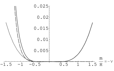
Figure 1: The solid line is $\langle\Psi^{2}\rangle|_{0}$, the dashed line is the bound state contribution ${}^{({bs})}\langle\Psi^{2}\rangle|_{0}$ (which is absent for $m>0$), and the dotted line corresponds to the KK contribution ${}^{(\textsc{kk})}\langle\Psi^{2}\rangle|_{0}$. These values are for $\mu=H$ and are expressed in units of $H^{3}$. For ${m}\to-3H/2$, the mass of the bound state vanishes like $m_{bs}^{2}\simeq 3(m+3H/2)H$, and $\langle\Psi^{2}\rangle|_{0}$ and ${}^{({bs})}\langle\Psi^{2}\rangle|_{0}$ grow like $\sim m_{bs}^{-2}$. In the same limit, the KK contribution grows but remains finite.

Figure 1 shows that in the limit $m_{bs}\to 0$ ($\nu\to 3/2$), the contribution from the KK modes (32) is negligible relative to the bound state contribution (31). In this limit, the bound state contribution diverges like ${}^{{bs}}\langle\Psi^{2}\rangle|_{0}\sim(9/16\pi^{2})(H^{5}/m_{bs}^{2})$, whereas the KK contribution grows but stays of order ${}^{\textsc{kk}}\langle\Psi^{2}\rangle|_{0}\sim(27/128\pi^{2})H^{3}$. Note that this statement does not depend on the choice of renormalization coefficients in (30) (also present in (31) and (32)). This result agrees with kks ; hts , where the contribution from the KK modes to the power spectrum of primordial fluctuations in the bulk inflaton model hs ; kks was also found to be small when the bound state is light.

Four dimensional conformal coupling

We see that the divergent part of (22) vanishes for $\nu=0,\pm 1/2$. In these cases, $\langle\Psi^{2}\rangle|$ does not depend on the renormalization scale $\mu$, and one can try to assign to $\langle\Psi^{2}\rangle|$ an unambiguous value. If we take the result from dimensional regularization (22), then $\langle\Psi^{2}\rangle|=0$ for $\nu=0$. In this case, the bound state is not normalizable (${\cal U}_{bs}=0$), and we conclude that the KK contribution also vanishes. In light of the relation between dimensional regularization and other schemes, this means that $\langle\Psi^{2}\rangle|_{0}$ in this case is a pure counter-term.

For $\nu=\pm 1/2$, Eq (22) gives

$$\langle\Psi^{2}\rangle\big{|}_{0}^{(\nu=\pm 1/2)}=-{H^{3}\over 64\pi^{2}}~{}.$$ (33)

For $\nu=-1/2$, there is no bound state, and the above is the contribution from the KK modes. The case $\nu=1/2$ corresponds to a bound state that effectively is conformally coupled in the four dimensional sense because $m^{2}_{{bs}}=2H^{2}=R_{(4)}/6$ (in 4D conformal coupling is for $\xi=1/6$). It is fortunate that in this case the five dimensional result is ’finite’ (there is no $\mu$ dependence) because the fluctuations of a conformally coupled scalar in dS are also finite vilenkinford , allowing for a straightforward comparison. The fluctuations for a conformally coupled scalar in four dimensional dS of unit radius give $1/48\pi^{2}$ vilenkinford . In our model, this contribution to the fluctuation has to be weighted by the wave function of the mode at the brane location ${\cal U}_{bs}^{2}|_{0}=\nu H^{n}$, so the bound state contributes as ${}^{({bs})}\langle\Psi^{2}\rangle|_{0}=H^{3}/96\pi^{2}$. The contribution from the KK modes then is ${}^{(kk)}\langle\Psi^{2}\rangle|_{0}=-(5/2)\;{}^{({bs})}\langle\Psi^{2}\rangle|_{0}$. Thus, the ’correction’ from the KK modes in this case is rather large. This could be anticipated because in this case the bound state is not very light, $m_{bs}=\sqrt{2}H$, so we do not expect it to dominate over the KK modes.

It is also worth noting that (33) is negative (because the KK contribution is negative). This is a typical outcome of the procedure of regularization necessary to make sense of divergent sums, even when all the terms are positive definite. So it should be interpreted with care. For instance, we can always choose a set of renormalization conditions (or make a finite renormalization of local counter-terms) so that $\langle\Psi^{2}\rangle$ becomes positive.

III Bulk–brane interaction and the effective potential

We shall consider a bi-scalar model

$$S=S_{\Psi}+S_{\varphi}+S_{int}$$ (34)

where $S_{\Psi}$ is given in (1), and for the brane field $\varphi$

$$S_{\varphi}=-{1\over 2}\int d^{4}x\sqrt{-h}\left[(\partial\varphi)^{2}+m_{\varphi}^{2}\varphi^{2}\right]~{},$$ (35)

where $h$ denotes the determinant of the induced metric on the brane. As for the interaction term, we take

$$S_{int}=-\int d^{4}x\sqrt{-h}\;\lambda\,\varphi^{2}\,\Psi^{2}|_{0}$$ (36)

where $\Psi^{2}|_{0}$ stands for the bulk field evaluated on the brane, and $\lambda$ is a coupling constant with dimensions of length.

III.1 Kaluzaz-Klein Reduction

The usual ’Kaluza-Klein decomposition’ (also called dimensional reduction) consists in inserting the KK ansatz $\Psi(z,x^{\mu})=\sum_{p}{\cal U}_{p}(z)\Psi_{p}(x^{\mu})$ with ${\cal U}_{p}(z)$ given by (7) and (5), introduce it into the action (34) and integrate out the extra dimension. Because of the orthonormality of the wavefunctions ${\cal U}_{p}(z)$, the resulting 4D action at quadratic order is

$$S=-{1\over 2}\int\sqrt{h}d^{4}x\;\left\{\left(\partial\varphi\right)^{2}+m_{\varphi}^{2}\varphi^{2}+\left(\partial\Psi_{bs}\right)^{2}+m_{bs}^{2}\Psi_{bs}^{2}~{}+~{}{\rm KK~{}modes}\right\}$$ (37)

where $m_{bs}^{2}=(3H/2)^{2}-{m}^{2}$. Having a light bound state $m_{bs}\ll H$, reduces to choosing ${m}$ close enough to $-3H/2$. One expects that this models some of the features of the minimally coupled case.

Restricting ourselves to configurations of constant $\varphi$, the interaction (36) can be taken into account by the replacement

$${m} \to{m}+\lambda\varphi^{2}~{}.$$ (38)

Then, the mass of the bound state is given by

$$m_{bs}^{2}=(3H/2)^{2}-\left({m}+\lambda\varphi^{2}\right)^{2}~{}.$$ (39)

and we can identify the classical potential as

$$V^{cl}={1\over 2}m_{bs}^{2}\Psi_{bs}^{2}+{1\over 2}m_{\varphi}^{2}\varphi^{2}={1\over 2}m_{0}^{2}\Psi_{bs}^{2}+{1\over 2}m_{\varphi}^{2}\varphi^{2}-{{m}\lambda}\,\varphi^{2}\Psi_{bs}^{2}-{1\over 2}\lambda^{2}\varphi^{4}\Psi_{bs}^{2}$$ (40)

where $m_{0}^{2}=\left(3H/2\right)^{2}-{m}^{2}$. Note that this potential contains a biquadratic interaction similar to the one in (36) with an effective (dimensionless) coupling constant given by $-m\lambda$ (recall that ${m}<0$). Aside from it, we notice an extra piece $\propto-\lambda^{2}\varphi^{4}\Psi_{bs}^{2}$. This term can be interpreted as a higher dimensional effect. To see this, note that it is crucial wether we consider the interaction (36) ’turned on’ at the 5D level (before doing the dimensional reduction), or at the 4D level (once it is already done). If it is considered turned off when doing the reduction, then $m_{bs}^{2}=(3H/2)^{2}-{m}^{2}$ and ${\cal U}_{bs}^{2}|_{0}\propto-{m}$ (see Eqns. (7) and (4)). To include the interaction, we insert this decomposition in (36) and the only interaction with the bound state $\Psi_{bs}$ is $\lambda\,{\cal U}_{bs}^{2}|_{0}\,\Psi_{bs}^{2}\,\varphi^{2}$, which agrees with the third term in (40). Thus, in the ’4D treatment’, the interaction is the bi-quadratic term only. If we consider (36) turned on at the 5D level, the spectrum (39) depends on $\lambda\varphi^{2}$. In particular ${\cal U}_{bs}^{2}|_{0}\propto-{m}-\lambda\varphi^{2}$, whence the new term arises. No correction is obtained unless the interaction is considered in the 5D sense, so we interpret the last term in (40) as a higher dimensional effect.

From the AdS/CFT correspondence adscft , the $\lambda^{2}\Psi_{bs}^{2}\varphi^{4}$ term can be interpreted as a quantum correction from the CFT, which agrees with the fact that it is of order $\lambda^{2}$. We leave for future investigation a detailed analysis of the correspondence in this setup. In Section III.2, we give further evidence for this interpretation, showing that one can reproduce the above potential using the method based on the geometrical projection of sms , as done in maedawands ; ls . In this approach, these terms arise from the square of the matter stress tensor (which are related to the conformal anomaly shiromizu ) and from the normal derivatives of $\Psi$ present in the bulk stress tensor maedawands . The analysis made in ls reveals that the effective potential obtained in this way agrees with that obtained by the mode decomposition, at least to leading order in the coupling to the brane ($m$, in our model).

Finally, note that the potential (40) is unbounded from below. This is not a problem, for two reasons. As we show in Section III.2, when we take into account all the terms in the effective potential as derived with the geometrical projection method maedawands ; ls , then it becomes bounded. Moreover, when the unbounded term becomes noticeable $(\lambda\varphi^{2}\gtrsim H)$ the bound state mass is comparable to $H$ and eventually disappears as a normalizable mode, meaning that the effective description (37) and (40) breaks down.

III.2 Geometrical Projection method

Here, we discuss how the previous effective theory can be partially re-derived by means of the geometrical projection of the equations of motion on the brane sms . The dilaton-gravity system in the BW was studied in maedawands , and the form of the effective potential for the four dimensional dilaton field was derived. In ls (see also shs ), this was compared to the mode spectrum, and the two approaches were found to agree at the linear level in the brane coupling ($m$ in our notation). In soda , the connection between this approach and the gradient expansion method kannosoda is described. References maedawands ; ls ; soda considered a minimally coupled field in the bulk. In this section we extend their analysis to the conformally coupled case.

In sms , the effective 4D Einstein equations were found to be

$${}^{(4)}G_{\mu\nu}=\kappa_{5}^{2}T^{Proj}_{\mu\nu}+8\pi G_{N}\;T^{Brane}_{\mu\nu}+\kappa_{5}^{4}\,\pi_{\mu\nu}-E_{\mu\nu}$$ (41)

where $T^{Brane}_{\mu\nu}$ is the matter stress tensor on the brane, $\pi_{\mu\nu}$ is quadratic in $T^{brane}_{\mu\nu}$, $E_{\mu\nu}$ is the projected Weyl tensor, and

$$T^{Proj}_{\mu\nu}\equiv\frac{2}{3}\left\{T^{Bulk}_{\rho\sigma}h_{~{}\mu}^{\rho}h_{~{}\nu}^{\sigma}+\big{(}T^{Bulk}_{\rho\sigma}n^{\rho}n^{\sigma}-{1\over 4}T^{Bulk\,\rho}_{~{}\rho}\big{)}h_{\mu\nu}\right\}~{}.$$ (42)

Here, $n^{\mu}$ is unit vector normal to the brane and $T^{Bulk}_{\rho\sigma}$ is the bulk stress tensor, and the effective Newton’s constant is $G_{N}=\kappa_{5}^{4}\,\sigma/48\pi$ where $\sigma$ is the brane tension.

The contribution to the stress tensor from a nonminimally coupled bulk field can be concisely written as bida ; saharian .

$$T_{\mu\nu}^{Bulk} = \partial_{\mu}\Psi\partial_{\nu}\Psi-{1\over 2}\;\left(\partial\Psi\right)^{2}g_{\mu\nu}+\left[-{1\over 2}M^{2}g_{\mu\nu}+\xi\left(G_{\mu\nu}+g_{\mu\nu}\Box-\nabla_{\mu}\nabla_{\nu}\right)\right]\Psi^{2}$$ (43)

$$T_{\mu\nu}^{Brane} = \delta(r-r_{0})\left[2\xi\,K_{\mu\nu}-h_{\mu\nu}\left({m}+2\xi K+2\xi n^{\mu}\partial_{\mu}\right)\right]\,\Psi^{2}~{},$$ (44)

where $h_{\mu\nu}$ is the induced metric on the brane, $G_{\mu\nu}$ is the bulk Einstein tensor, and $r$ denotes the normal coordinate. See fulling ; romeosaharian ; saharianWightman and references therein for the relevance of the surface terms in Casimir energy computations. Note that in these expressions we didn’t use the equations of motion. For $M={m}=0$ and $\xi=n/4(n+1)$, and using the equations of motion, it is easy to check that both components are traceless. Hence, the projected bulk tensor that enters into the effective Einstein equations is

$$T_{\mu\nu}^{Proj}={2\over 3}\left[h^{\mu}_{i}h^{\nu}_{j}T_{\mu\nu}^{Bulk}+h_{\mu\nu}n^{\mu}n^{\nu}T_{\mu\nu}^{Bulk}\right]$$

The first two terms in (43) only contribute 4-dimensional derivative terms to $T^{Proj}_{\mu\nu}$. Then, the contribution to the effective potential from $T^{Bulk}$ is

$$T^{Proj}_{\mu\nu} ={2\over 3}\xi\,h_{\mu\nu}\left[2G_{rr}\Psi^{2}+4\xi R\Psi^{2}+2(\partial_{r}\Psi)^{2}-2\Psi\partial_{r}^{2}\Psi-{1\over 2}K\Psi\partial_{r}\Psi+\dots\right]$$ (45)

$$={2\over 3}\xi\,h_{\mu\nu}\left[-{3\over\ell^{2}}+2yH\left(m+{3\over 2}yH\right)+\dots\right]\Psi^{2}$$ (46)

$$=-{1\over 2}h_{\mu\nu}\left[-{3\over 4}H^{2}-{1\over 2}m\,yH+\dots\right]\Psi^{2}$$ (47)

where in the first equation we used the equation of motion $\Box\Psi=\xi R\Psi$ and $K_{\mu\nu}=Kh_{\mu\nu}/4$ given that the brane is maximally symmetric. In the second, we used the boundary condition $\partial_{r}\Psi|_{r=r_{0}^{-}}=-({m}+2\xi K)\Psi$, Eq. (29) and the equation of motion for the background. For the second normal derivative we have taken $\partial_{r}^{2}\Psi=({m}+2\xi K)^{2}\Psi$ maedawands (see also ls ), and the dots denote four-dimensional derivative terms. The brane stress tensor is

$$T_{\mu\nu}^{Brane}=-\delta(r-r_{0})h_{\mu\nu}\left[\sigma+{{m}\over 4}\,\Psi^{2}\right]\equiv-\delta(r-r_{0})h_{\mu\nu}\,\left[\sigma+V_{0}\right]~{},$$

where we have included the tension term. Thus, the contribution to the effective potential from the brane stress tensor is

$${\kappa_{5}^{2}\over 12}\left(\sigma+V_{0}\right)^{2}={\kappa_{5}^{2}\over 12}\left(2\sigma V_{0}+V_{0}^{2}\right)+const={1\over 2}\left[{1\over 2}{m}yH\Psi^{2}+{\kappa_{5}^{2}\over 6}{m^{2}\over 16}\Psi^{4}+const\right]~{}.$$ (48)

From this and Eq. (45), we find that the terms linear in the coupling to the brane ${m}$ in the effective mass squared cancel. This agrees with the form of the bound state mass (39), and also happens for the minimally coupled field ls . The agreement between this treatment and that of Section III is not apparent in the higher order terms (neither the zeroth order term, proportional to $H^{2}$, even though this term vanishes in the flat brane limit). Still, the geometrical projection method is illustrative because it unveils the presence of interaction terms like $\Psi^{4}$ term in (48) that cannot be obtained from the mass spectrum alone. Furthermore, the presence of $V_{0}^{2}$ in (48) shows that the effective potential is bounded from below.

IV 1-loop effective potential

The 1-loop effective potential for $\varphi$, induced by the bulk field $\Psi$ can be obtained by the following procedure. The equation of motion for $\varphi$ is

$$[\Box-m_{\varphi}^{2}-2\lambda\Psi^{2}|_{0}]\varphi=0.$$ (49)

We split the brane field as $\varphi=\varphi_{c}+\delta\varphi$, where $\varphi_{c}$ represents the vev in the true vacuum. If $\varphi$ acquires a vev, then the effective brane mass term for $\Psi$ is

$${m}+2\xi K+\lambda\varphi_{c}^{2}~{}.$$

The one loop approximation consists in replacing $\Psi^{2}|_{0}$ by $\langle\Psi^{2}\rangle|_{0}$ in (49), where the latter is computed with the effective brane mass term above. This is obtained by making the replacement (38) in (30). Then, from Eq. (49) we identify the 1-loop effective potential as

$${\partial V_{\rm eff}\over\partial\varphi_{c}}\equiv m^{2}_{\varphi}\varphi_{c}+2\lambda\varphi_{c}\;\langle\Psi^{2}\rangle|_{0}(\varphi_{c})$$ (50)

Needless to say, $\langle\Psi^{2}\rangle|_{0}$ and $V_{\rm eff}(\varphi_{c})$ above are understood as renormalized values, so they depend on the renormalization conditions that one imposes.

We stress that we shall integrate out only the KK continuum, first of all because this is what we are interested in. Furthermore, a complete discussion of the effect of a very light mode would require going to higher loops, and this is out of the scope of this paper. According to the split of $\langle\Psi^{2}\rangle$ made in Section II.3, the contribution from the KK modes is given by

$${\partial V^{\textsc{kk}}\over\partial\varphi_{c}}\equiv 2\lambda\varphi_{c}\;{}^{(\textsc{kk})}\langle\Psi^{2}\rangle|_{0}(\varphi_{c})~{}.$$ (51)

Because the 1-loop KK contribution depends only on $\varphi_{c}$, the total effective potential takes the form

$$V_{\rm eff}=V^{cl}\big{(}\varphi_{c},\Psi_{bs}\big{)}+V^{\textsc{kk}}\big{(}\varphi_{c}\big{)}~{},$$ (52)

where $V^{cl}$ is given in (40). We shall impose the following renormalization conditions

$$V^{\textsc{kk}}|_{\varphi=0} =0$$ (53)

$$\partial_{\varphi_{c}}^{2}V^{\textsc{kk}}|_{\varphi=0} =0$$ (54)

The first condition ensures that in the $\varphi_{c}=0$ vacuum, the cosmological constant is the same as in the background. The second demands that $V_{\rm eff}^{\prime\prime}(\varphi)$ coincides with the mass at tree level $m_{\varphi}^{2}$, at $\varphi_{c}=0$.

We showed in Section II that $\langle\Psi^{2}\rangle|_{0}$ is defined up to the four constants $A$, $B$, $C$ and $\mu$ in (30). The equations (53) fixes one of them. We will assume that the remaining renormalization constants are of order one in the natural units of the problem. This leads to the potential depicted in Fig. 2 for natural choices of the parameters. For $\lambda\varphi^{2}\ll H$, this potential can be parametrized as

$$V_{\rm eff}={1\over 2}m_{\varphi}^{2}\varphi^{2}-{1\over 4}a_{4}\;H^{2}(\lambda\varphi^{2})^{2}+{1\over 6}a_{6}\;H(\lambda\varphi^{2})^{3}+\dots$$ (55)

where $a_{4}$ and $a_{6}$ are numerical coefficients suppressed by 1-loop factors (e.g. $1/64\pi^{2}$, see Eq. (30)) and are typically of order $10^{-2}$–$10^{-3}$ . Physically, the fluctuations ${}^{(\textsc{kk})}\langle\Psi^{2}\rangle$ increase for $\varphi\to 0$, because in this limit there is a massless mode in the spectrum. This implies a negative slope at $\varphi=0$ both in ${}^{(\textsc{kk})}\langle\Psi^{2}\rangle$ and in $V^{\textsc{kk}}$. That is why we take the $\varphi^{4}$ term negative. The extrema are located at

$$\lambda\,\varphi^{2}={a_{4}H\over 2a_{6}}\pm\sqrt{\left({a_{4}H\over 2a_{6}}\right)^{2}-{m_{\varphi}^{2}\over\lambda H\,a_{6}}},$$ (56)

the minus sign corresponding to the maximum, and the plus to the new vacuum. This appears only for light enough $\varphi$ or conversely when the interaction (36) is strong enough,

$$m_{\varphi}^{2}<\lambda H{a_{4}^{2}\over 4a_{6}}H^{2}~{}.$$ (57)

From (56), we see that the location of the new vacuum is such that

$$\lambda\langle\varphi\rangle^{2}\gtrsim{a_{4}\over a_{6}}H~{},$$

and in the absence of fine tunings one expects this to exceed the critical value $3H/2$. In this case, the parameter $\nu=-{m}-\lambda\varphi^{2}$ becomes negative, which renders the bound state of $\Psi$ unnormalizable (see Eq. (7)). In this situation, this mode becomes a quasi-normal mode with decay width given by $\nu$, and it decays to the KK modes rubakov . Hence, the new minimum represents the true vacuum, and the original one is at most meta-stable. From (55) that the value of the potential at the new minimum typically is smaller than at the $\varphi=0$. At the new minimum, the quadratic term in (55) can be neglected because it is only comparable to the quartic term at the location of the maximum. Hence, an order-of-magnitude estimate of the decrease in the potential at the true vacuum is

$$\delta V\sim-{1\over 12}{a_{4}^{3}\over a_{6}^{2}}H^{4}~{},$$

which is suppressed respect to $H^{4}$ by one 1-loop factor. This gives a small correction to the background potential or cosmological constant that is driving inflation, so a transition to the true vacuum does not imply that inflation stops. It only affects the spectrum of the bulk fields.

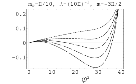
Figure 2: Form of the effective potential $V_{\rm eff}(\varphi)$ for typical values of the parameters corresponding to the conformally coupled bulk field. We plot the difference with respect to the background vacuum energy density in units of $H^{4}$, and we represent it on the axis $\Psi_{bs}=0$. The dotted line is with $\log(\mu/H)=-0.8$. For longer dashing, the logarithm is subsequently increased by $0.2$. We see how $V_{\rm eff}(\varphi)$ tends to acquire a true vacuum away from $\varphi=0$. Positive values of $\log(\mu/H)$ lead to more negative potential.

V Conclusions

We have shown that the Kaluza-Klein excitations can considerably modify the dynamics when interactions are included. We have considered a bulk scalar field $\Psi$ coupled on the brane to a 4D scalar field $\varphi$ with a bi-quadratic interaction on the brane of the form (36) taking as the background the RSII space rsII with an inflating brane. The bulk field $\Psi$ has an almost massless mode, the ’bound state’. We have computed the effective potential $V_{\rm eff}(\varphi)$ induced by the KK modes. The potential $V_{\rm eff}(\varphi)$ typically develops a minimum at a value of $\varphi$ for which the bound state of $\Psi$ is no longer normalizable. For natural choices of the renormalization parameters, the potential in the new vacuum is smaller than in the original one. This indicates that the vacuum $\varphi=0$ is meta-stable. In the true vacuum, the former bound state mode becomes unstable– it acquires a finite width and decays into bulk modes rubakov .

Intuitively, this happens because when the bound state of $\Psi$ is light, then the fluctuations $\langle\Psi^{2}\rangle$ become large, as long as the brane is inflating. Due to the interaction (36), $\langle\Psi^{2}\rangle$ act as an effective mass term for $\varphi$. The configuration with larger effective mass is disfavored, hence the brane field $\varphi$ is driven away from $\varphi=0$ by the quantum effects of the bulk field $\varphi$.

In this model, the KK modes seem to affect the dynamics considerably. The reason is that in the one brane model with an infinite extra dimension, the lightest KK mass is of order of the Hubble constant, which is relatively light. Moreover, it is natural that the fluctuations of the KK modes are sensitive to how light is the lightest mode because, after all, they are part of the same 5D field and the fluctuations have to increase in this limit. Finally, the contribution to $\langle\Psi^{2}\rangle$ from the bound state is even larger than that of the KK modes (see Fig. 1, and kks ; shs ), so if we include it then the instability is even stronger.

We also comment on a number of technical issues related to the method used to obtain the 1-loop result for the quantum fluctuations on the brane $\langle\Psi^{2}\rangle|_{0}$ (30), from which we derive the effective potential $V_{\rm eff}(\varphi)$. One way to compute $\langle\Psi^{2}\rangle|_{0}$ is by taking into account the brane thickness, where this feature is not expected to appear. In this article, we have resorted to the thin wall approximation. A generic consequence of this is that the vev of the field fluctuations $\langle\Psi^{2}\rangle$ blow up close to the brane. We showed that the field fluctuations on the brane $\langle\Psi^{2}\rangle|_{0}$ are well defined up to mass and extrinsic curvature counter-terms. Furthermore, we found that the renormalized values of fluctuations on the brane $\langle\Psi^{2}\rangle|_{0}$ and in the bulk $\langle\Psi^{2}\rangle(z)$ (close enough to the brane) coincide up to finite renormalization of mass and extrinsic curvature counter-terms. This is what one would expect to happen, and was previously noticed in ns for vanishing brane mass. The equivalence between $\langle\Psi^{2}\rangle|_{0}$ and $\langle\Psi^{2}\rangle(z)$ in the less trivial case discussed here provides further evidence on the validity of the thin wall approximation.

Our computation of $\langle\Psi^{2}\rangle|_{0}$ shows that the KK continuum behaves like a purely-decaying mode of a scalar field. For the range of parameters that give rise to a normalizable bound state, the KK mode contribution exactly cancels (up to finite renormalization of mass terms) the decaying-mode contribution of the bound state. For choices of the parameters leading to no bound state, the KK contribution behaves like the quasi-normal mode of the 5D field $\Psi$, which is ’purely decaying’ in the case of conformal coupling. We leave for future investigation the analysis of bulk scalar fields with generic mass and non-minimal coupling. Also, our computation shows that the the bound state contribution (31) to the field fluctuations on the brane $\langle\Psi^{2}\rangle|_{0}$ dominate over the KK contribution (32)) for $m_{bs}\ll H$. This agrees with the results of kks ; hts , where the contribution to the power spectrum from the KK modes was found to be negligible. One expects that this holds also for generic bulk fields, though the analysis is slightly more technical and is left for the future.

Our computation is relevant to the bulk inflaton model hs ; kks where $\Psi$ plays the role of the a 5D field that drives inflation. This field is assumed to have a light mode, whose fluctuations seed the universe with the primordial perturbations. Our result implies that the phase when $\Psi$ has a light mode is limited by the instability of this vacuum. It seems that the instability described here could places some constraints on the model, which for instance depend on the mass of the brane field $m_{\varphi}$ and the coupling constant $\lambda$. It is not the purpose of this article to discuss the details of these constraints, or the way how the decay of the false vacuum proceeds, since they seem quite model-dependent. On the other hand, it seems that this phenomenon can be extended to other brane models. Whenever the brane is inflating, there is a bulk field with a light mode and it is coupled to brane fields, the effective potential should favor a vacuum where the fluctuations of the bulk field are not so large, which precisely corresponds to not having a very light mode.

Appendix A Conformal Transformations

The form of $\langle\Psi^{2}\rangle$ for the flat ball (the interior of a spherical cavity in flat space) was discussed in pt . Using the flat radial coordinate $\rho$, the metric for the flat ball is

$$ds_{{({\rm flat})}}^{2}=d\rho^{2}+\rho^{2}\;dS_{(n+1)}^{2},$$ (58)

where $dS_{(n+1)}^{2}$ is the metric on a $n+1$ dimensional de Sitter space. In terms of this coordinate, the renormalized Green function for a conformally coupled field with no brane mass in the de Sitter invariant vacuum is pt

$$G^{(1)}_{({\rm flat})}(x,x^{\prime}) ={2\over nS_{(n+1)}}\left({1\over\rho_{0}^{2}+(\rho\rho^{\prime}/\rho_{0})^{2}-2\rho\rho^{\prime}\cos\zeta}\right)^{{n\over 2}},$$ (59)

where $\rho_{0}$ is the location of the brane, $\zeta$ is the geodesic distance in $dS$ space and $S_{(n+1)}=2\pi^{n/2+1}/\Gamma(n/2+1)$ is the volume of a unit $n+1$ dimensional sphere. Equation (59) can be easily derived by the method of images. The coincidence limit of this expression is finite in the bulk, so we readily obtain

$${}^{{({\rm flat})}}\langle\Psi^{2}\rangle(x)={1\over nS_{(n+1)}}\,\left({\rho_{0}\over\rho_{0}^{2}-\rho^{2}}\right)^{n}.$$ (60)

Now consider a bulk space of the form

$$ds^{2}_{(a)}=dr^{2}+a^{2}(r)dS^{2}_{(n+1)}.$$ (61)

Clearly, this is conformally related to flat space,

$$ds^{2}_{(a)}=\Omega^{2}\,ds^{2}_{(0)},$$

with $\Omega=a/\rho=\cosh^{2}\left(r/2\ell\right)$. Note that this conformal factor is finite everywhere. The relationship between the radial coordinate $r$ and the flat coordinate $\rho$ is

$$\ln\left(\rho_{0}/\rho\right)=\int_{r}^{r_{0}}{dr\over a(r)}\equiv z,$$ (62)

and we have introduced the conformal coordinate $z$, in terms of which the brane sits at $z=0$, and $r=\rho=0$ corresponds to $z\to\infty$.

On the other hand, the Green function in the space (61) for the conformally coupled scalar in the conformal vacuum is

$$G^{(1)}_{(a)}(x,x^{\prime})=\left[\Omega(x)\Omega(x^{\prime})\right]^{-n/2}\,G^{(1)}_{({\rm flat})}(x,x^{\prime})$$ (63)

Hence, in the space (61) we obtain for this vacuum

$${}^{(a)}\langle\Psi^{2}\rangle(x)={a^{-n}\over nS_{(n+1)}}\left({\rho_{0}\,\rho\over\rho_{0}^{2}-\rho^{2}}\right)^{n}={\big{(}2\,a\,\sinh{z}\big{)}^{-n}\over nS_{(n+1)}}~{},$$ (64)

which agrees with ns . This means that the procedure to compute $\langle\Psi^{2}\rangle$ used in ns , based on a conformal transformation to the cylinder adding a regulating brane and then sending it to conformal infinity, works when computing local quantities like $\langle\Psi^{2}\rangle(z)$. Recently, it was shown in fkns that this procedure does not reproduce the correct results for global quantities such as the effective action. The reason seems to be that by introducing the second brane, one modifies the topology (even in the limit when it is sent to infinity). However, it seems reasonable that this procedure still works to compute local quantities. Note that the method used in this Appendix also makes use of a conformal transformation. However, it is perfectly regular at all points, and the topology is not altered.

We can apply the same method to compute $G$ and $\langle\Psi^{2}\rangle$ in the case when we break conformal invariance in one point, on the brane. The boundary condition in the original AdS space is

$$[n^{\mu}\partial_{\mu}-2\xi_{c}K-{m}]\Psi|_{0}=0$$

where $|_{0}$ denotes evaluation on the brane. Because of the mass term, this is not conformally invariant. However, the conformal factor that links AdS with flat space is constant on $r=$const. surfaces, so the boundary condition can be written in the same form if we rescale the mass term as ${m}\to{m}/\Omega_{0}$. Since the Hubble constant on the brane $H=a_{0}^{-1}$ scales precisely in the same way, the parameter $\nu=-{m}/H$ (see Eq (4)) does not scale. Hence, for $M=0$, $\xi=3/16$ and ${m}\neq 0$, the form of $\langle\Psi^{2}\rangle$ is the same as (16) for any space conformally related to the flat ball.

Finally, we shall comment on one further check of (30). In flatball , the determinant of the Laplace operator for a scalar field in the flat ball with Robin boundary conditions on the boundary was computed (see kirsten for the computation in more general situations). This is equivalent to the effective potential induced by a bulk field for any nonminimal coupling, as a function of the boundary condition parameter. As discussed above, this space is conformal to the AdS ball. The difference between the effective potential of a given field in conformally related spaces is known as the cocycle function, and can be written in terms of the geometrical invariants of both spaces gpt ; gpt2 ; da , through the Seeley-DeWitt coefficients. It also depends on the field parameters (bulk and brane masses, etc). It can be easily shown (see e.g. a5 ) that the dependence is polynomial in the boundary mass. Thus, the dependence in ${m}$ of the cocycle function connecting the flat ball and the AdS ball reduces to pure counter-terms and can be ignored. Indeed, it can easily be checked that the effective potential found in flatball satisfies (52) up to polynomial terms in ${m}$.

References

-
(1)
N. Arkani-Hamed, S. Dimopoulos, G. Dvali, Phys. Lett. B429 263;
I. Antoniadis, N. Arkani-Hamed, S. Dimopoulos, G. Dvali, ibid. B436 257. - (2) L. Randall and R. Sundrum, Phys. Rev. Lett. 83, 3370 (1999).
- (3) L. Randall and R. Sundrum, Phys. Rev. Lett. 83, 4690 (1999).
- (4) J. Garriga and M. Sasaki, Phys. Rev. D 62, 043523 (2000).
- (5) S. Kobayashi, K. Koyama and J. Soda, Phys. Lett. B 501, 157 (2001).
- (6) Y. Himemoto and M. Sasaki, Phys. Rev. D 63, 044015 (2001).
- (7) N. Sago, Y. Himemoto and M. Sasaki, Phys. Rev. D 65, 024014 (2002).
- (8) Y. Himemoto, T. Tanaka and M. Sasaki, Phys. Rev. D 65, 104020 (2002).
- (9) J. Garriga, O. Pujolàs and T. Tanaka, Nucl. Phys. B 605, 192 (2001).
- (10) A. Flachi, D.J. Toms, Nucl. Phys. B610 (2001) 144.
- (11) W.D. Goldberger, I.Z. Rothstein, Phys. Lett. B491 (2000) 339.
- (12) J. Garriga, O. Pujolàs and T. Tanaka, Nucl. Phys. B 655, 127 (2003).
- (13) A. Flachi, J. Garriga, O. Pujolàs and T. Tanaka, JHEP 0308, 053 (2003).
- (14) A. Flachi and O. Pujolàs, Phys. Rev. D 68, 025023 (2003).
- (15) J. Garriga and A. Pomarol, Phys. Lett. B 560, 91 (2003).
- (16) I. Brevik, K. A. Milton, S. Nojiri and S. D. Odintsov, Nucl. Phys. B 599, 305 (2001).
- (17) A. A. Saharian and M. R. Setare, Phys. Lett. B 552, 119 (2003).
-
(18)
W. Naylor and M. Sasaki,
Phys. Lett. B 542, 289 (2002);
E. Elizalde, S. Nojiri, S. D. Odintsov and S. Ogushi, Phys. Rev. D 67, 063515 (2003);
I. G. Moss, W. Naylor, W. Santiago-German and M. Sasaki, Phys. Rev. D 67, 125010 (2003);
I. Brevik, K. A. Milton, S. Nojiri and S. D. Odintsov, Nucl. Phys. B 599, 305 (2001). - (19) S. Nojiri and S. D. Odintsov, JCAP 0306, 004 (2003).
- (20) E. Elizalde, S. Nojiri, S. D. Odintsov and S. Ogushi, Phys. Rev. D 67, 063515 (2003).
- (21) W. Naylor and M. Sasaki, Prog. Theor. Phys. 113, 535 (2005).
- (22) A. Flachi, A. Knapman, W. Naylor and M. Sasaki, Phys. Rev. D 70, 124011 (2004).
- (23) O. Pujolàs and T. Tanaka, JCAP 0412, 009 (2004).
- (24) X. Montes, Int. J. Theor. Phys. 38, 3091 (1999).
- (25) N. D. Birrell and P. C. W. Davies, “Quantum Fields In Curved Space,” Cambridge University Press.
- (26) D. Deutsch and P. Candelas, Phys. Rev. D 20, 3063 (1979).
- (27) G. Kennedy, R. Critchley and J. S. Dowker, Annals Phys. 125, 346 (1980).
- (28) A. Romeo and A. A. Saharian, J. Phys. A 35, 1297 (2002).
- (29) S. A. Fulling, J. Phys. A 36, 6529 (2003).
- (30) A. Knapman and D. J. Toms, Phys. Rev. D 69, 044023 (2004).
-
(31)
N. Graham and K. D. Olum,
Phys. Rev. D 67, 085014 (2003)
[Erratum-ibid. D 69, 109901 (2004)];
K. D. Olum and N. Graham, Phys. Lett. B 554, 175 (2003). - (32) A. Vilenkin and L. H. Ford, Phys. Rev. D 26, 1231 (1982).
- (33) T. S. Bunch and P. C. W. Davies, Proc. Roy. Soc. Lond. A 360 (1978) 117.
- (34) T. Shiromizu, K. i. Maeda and M. Sasaki, Phys. Rev. D 62, 024012 (2000).
- (35) K. i. Maeda and D. Wands, Phys. Rev. D 62, 124009 (2000).
- (36) D. Langlois and M. Sasaki, Phys. Rev. D 68, 064012 (2003).
- (37) S. Kanno and J. Soda, Gen. Rel. Grav. 36, 689 (2004).
- (38) S. Kanno and J. Soda, Phys. Rev. D 66, 043526 (2002).
- (39) S. L. Dubovsky, V. A. Rubakov and P. G. Tinyakov, Phys. Rev. D 62, 105011 (2000).
-
(40)
J. M. Maldacena,
Adv. Theor. Math. Phys. 2, 231 (1998)
[Int. J. Theor. Phys. 38, 1113 (1999)]
;
E. Witten, Adv. Theor. Math. Phys. 2, 253 (1998). -
(41)
T. Shiromizu and D. Ida,
Phys. Rev. D 64, 044015 (2001)
;
T. Shiromizu, T. Torii and D. Ida, JHEP 0203, 007 (2002). - (42) A. A. Saharian, Phys. Rev. D 69, 085005 (2004).
- (43) A. A. Saharian, Nucl. Phys. B 712, 196 (2005).
-
(44)
M. Bordag, B. Geyer, K. Kirsten and E. Elizalde,
Commun. Math. Phys. 179, 215 (1996)
;
J. S. Dowker, Class. Quant. Grav. 13, 585 (1996). - (45) M. Bordag, K. Kirsten and S. Dowker, Commun. Math. Phys. 182, 371 (1996).
- (46) J. S. Dowker and J. S. Apps, Class. Quant. Grav. 12, 1363 (1995).
- (47) K. Kirsten, Class. Quant. Grav. 15, L5 (1998).