Effective dynamics of an electrically charged string with a current

Abstract

Equations of motion for an electrically charged string with a current in an external electromagnetic field with regard to the first correction due to the self-action are derived. It is shown that the reparametrization invariance of the free action of the string imposes constraints on the possible form of the current. The effective equations of motion are obtained for an absolutely elastic charged string in the form of a ring (circle). Equations for the external electromagnetic fields that admit stationary states of such a ring are revealed. Solutions to the effective equations of motion of an absolutely elastic charged ring in the absence of external fields as well as in an external uniform magnetic field are obtained. In the latter case, the frequency at which one can observe radiation emitted by the ring is evaluated. A model of an absolutely nonstretchable charged string with a current is proposed. The effective equations of motion are derived within this model, and a class of solutions to these equations is found.

1 Introduction

The description of the effective dynamics of electrically charged low-dimensional objects, such as particles, strings, and membranes, is one of traditional problems in classical electrodynamics. The application of such models allows one to considerably simplify the solving of the system of Maxwell–Lorentz integrodifferential equations. For a nonrelativistic charged particle, the effective equations of motion were obtained as early as by Lorentz [1]. The relativistic generalization of the Lorentz equations was derived by Dirac [2]. At present, the effective equations of motion are known for a point charge in a curved background space–time [3], for a spinning particle [4, 5], for a massive particle in higher dimensions [6, 7], and for a massless charged particle in the four-dimensional space–time [8]. The general scheme for the description of the self-action of electric currents in the string models is given in [9]. In [10], the general theory of moving electrically charged relativistic membranes is described.

In the present paper, we give an approximate (neglecting the effect of radiative friction) Poincaré-invariant description of the effective dynamics of a thin electrically charged string with a current. The importance of studying the effective dynamics of such strings is beyond doubt because of the numerous applications, both in practice and theoretical models, of extended charged and / or conducting objects with negligible transverse dimensions. For instance, the effective equations of motion obtained in Section 2 are applied to two specific models of strings in Sections 3 and 4. In Section 3 we consider the effective dynamics of an absolutely elastic ring-shaped charged string. This model describes the dynamics of a high-current beam of charged particles that move along a circle. In Section 4, we study the effective dynamics of an absolutely nonstretchable charged string with a current. In Section 2, we derive the effective equations of motion for a charged string with a current and discuss some of their properties; in particular, in the case of a reparametrization-invariant free action of a string, we find the generators of gauge transformations and the constraints on the possible form of the current that flows along the string.

We will describe a charged string within the model of an infinitely thin string. It is well known that the self-action of such a string leads to a diverging expression for the force of the self-action, because infinitely close points of an infinitely thin charged string interact with infinite force. The regularization procedure, whose physical meaning consists in “smearing” a singular source of the electromagnetic field, allows one to represent the self-action force as an asymptotic series in the regularization parameter – the cross-section radius of the string – which contains one logarithmically divergent term. The smaller the cross-section radius of the string, the greater the contribution of this divergent term to the self-action force. For a sufficiently thin string, one may neglect other terms of the asymptotic series to obtain effective equations of motion for a thin charged string in the form of a system of differential equations rather than integrodifferential equations, as in the case when all terms of the asymptotic series are taken into account. Similar equations are obtained when describing the effective dynamics of cosmic strings (see review [12]).

2 A charged string with a current

In this section, we find the leading contribution of the self-action of an electrically charged string with a current and derive equations of motion for the string in an external field with regard to this correction. We show that the requirement of the reparametrization invariance of the free action of a string imposes constraints on the possible form of the current flowing through the string.

Suppose given a closed string $N$ with coordinates $\{\tau,\sigma\}$, $\sigma\in[0,2\pi)$, that is embedded by a smooth mapping $x(\tau,\sigma)$ into the Minkowski space $\mathbb{R}^{3,1}$ with coordinates $\{x^{\mu}\}$, $\mu=0,\ldots,3$ and the metric $\eta_{\mu\nu}=diag(1,-1,-1,-1)$. Suppose that $e(\tau,\sigma)$ is a vector density defined on the string $N$ that characterizes the electric current flowing through the string. Then, from the viewpoint of an ambient space, the current density is given by (see, for example, [10])

$$j^{\mu}(x)=c\int{\delta^{4}(x-x(\tau,\sigma))e^{i}(\tau,\sigma)\partial_{i}x^{\mu}(\tau,\sigma)d\tau d\sigma},$$ (1)

where $c$ is the velocity of light; it is obvious that the charge conservation law $\partial_{\mu}j^{\mu}=0$ immediately implies $\partial_{i}e^{i}=0$. Hereupon, the Latin indices run through the values $0,1$ and correspond to $\tau$ and $\sigma$ respectively.

Let us introduce a nondegenerate symmetric scalar product in a linear space of $n$-forms on $\mathbb{R}^{3,1}$ as follows:

$$\langle X,Y\rangle=n!\int\limits_{\mathbb{R}^{3,1}}{X\wedge*Y}=\int\limits_{\mathbb{R}^{3,1}}{X_{\mu_{1}\ldots\mu_{n}}Y^{\mu_{1}\ldots\mu_{n}}d^{4}x},$$ (2)

here $*$ is the Hodge operator that sends $n$-forms to $(4-n)$-forms, and $\wedge$ denotes the exterior product of forms. In these terms, the action of the model in question is expressed as

$$S[A,x]=-\frac{1}{8\pi c}\langle A,\delta dA\rangle-\frac{1}{c^{2}}\langle j,A\rangle+S_{0}[x],$$ (3)

where $d$ is the exterior differential, $\delta=*d*$, $A_{\mu}$ is the $4$-potential of the electromagnetic field, and $S_{0}[x]$ is the action that describes the free dynamics of the string. The equations of motion for action (3) are given by

$$\delta F=-\frac{4\pi}{c}j,\;\;\;\;\;\frac{\delta S_{0}[x]}{\delta x^{\mu}}=\frac{1}{c^{2}}\langle\frac{\delta j[x]}{\delta x^{\mu}},A\rangle=\frac{1}{c}F_{\mu\nu}e^{i}\partial_{i}x^{\nu},$$ (4)

where $F=dA$ is the strength tensor of the electromagnetic field.

To obtain effective equations of motion of a string, we should solve the Maxwell equations for an arbitrary configuration of the string and substitute the solutions of these equations into the expression for the Lorentz force. This yields an ill-defined (divergent) expression for the self-action force of the string:

$$F^{rr}_{\mu}[x]=-\frac{4\pi}{c^{3}}\langle\frac{\delta j[x]}{\delta x^{\mu}},Gj[x]\rangle,$$ (5)

where $G$ is an operator whose kernel is a retarded Green’s function. Applying a regularization procedure [13] to this expression, we obtain an asymptotic series in the regularization parameter that contains one logarithmically divergent term. The regularization parameter makes the sense of the cross-section radius of the string; when this radius tends to zero, the radiation reaction force diverges. If the cross-section radius is small but finite, then this divergent term makes the most essential contribution to the self-action force; moreover, the smaller the cross-section radius, the larger this contribution.

Using the formalism developed in [13] we can easily show that the logarithmically divergent term that arises in the expression for the self-action force can be obtained by varying the action with the Lagrangian

$$L^{sing}=-\frac{1}{c}\left.\frac{e^{i}\partial_{i}x_{\mu}e^{j}\partial_{j}x^{\mu}}{\sqrt{|h|}}\,2\ln\frac{\Lambda}{\varepsilon}\right|_{\varepsilon\rightarrow 0}=-\frac{1}{c}\left.\frac{e^{2}}{\sqrt{|h|}}\,2\ln\frac{\Lambda}{\varepsilon}\right|_{\varepsilon\rightarrow 0},$$ (6)

where $e^{2}=e^{i}e^{j}h_{ij}$, $h_{ij}=\partial_{i}x_{\mu}\partial_{j}x^{\mu}$ is the induced metric on the string, $h=\det h_{ij}$, the parameter $\Lambda$ characterizes the cut-off of the integral at the upper limit (its magnitude is on the order of the string length), and $\varepsilon$ is the cut-off parameter of the integral at the lower limit (its magnitude is on the order of the cross-section radius of the string).

Let us introduce a vector field $V^{i}=e^{i}/\sqrt{|h|}$ and a $1$-form $\upsilon_{i}=h_{ij}V^{i}$. Then, neglecting the finite part of the radiation reaction force, we obtain the following effective equations of motion of the string:

$$\frac{\delta S_{0}[x]}{\delta x^{\mu}}=\frac{\chi}{c}(T^{ij}\nabla_{ij}x_{\mu}+\nabla_{i}T^{ij}\partial_{j}x_{\mu})\sqrt{|h|}+\frac{1}{c}F_{\mu\nu}e^{i}\partial_{i}x^{\nu},\;\;\;\;\;T^{ij}=(V^{2}h^{ij}-2V^{i}V^{j}),$$ (7)

where $\chi=2\ln(\Lambda/\varepsilon)$ is a dimensionless constant, $F_{\mu\nu}$is the strength tensor of the external electromagnetic field, and $\nabla_{i}$ is a connection compatible with the metric $h_{ij}$. The traceless tensor $T^{ij}$ represents the density of the energy–momentum tensor corresponding to Lagrangian (6); i.e.,

$$T^{sing}_{\mu\nu}=\frac{\chi}{c}\int{\delta^{4}(x-x(\tau,\sigma))T^{ij}\partial_{i}x_{\mu}\partial_{j}x_{\nu}\sqrt{|h|}d\tau d\sigma}.$$ (8)

The tracelessness of the tensors $T^{ij}$ and $T^{sing}_{\mu\nu}$ follows from the conformal invariance of Lagrangian (6).

If the free action $S_{0}[x]$ of the string is reparametrization-invariant, then the equations of motion (7) possess a “residual” reparametrization invariance, which implies that the equations are orthogonal to the vector $V^{i}\partial_{i}x^{\mu}$. In addition, we have

$$\nabla_{k}T^{k}_{i}=-2i_{V}d\upsilon_{i}=-\chi^{-1}\partial_{i}x^{\mu}F_{\mu\nu}V^{k}\partial_{k}x^{\nu}.$$ (9)

In particular, in the absence of an external field, the above equality and the charge conservation law $\nabla_{i}V^{i}=0$ imply

$$d\upsilon=0,\;\;\;\;\;\delta\upsilon=0,$$ (10)

i.e. $\upsilon$ is a harmonic 1-form. If the closed string has no self-intersections, Eqs. (10) are easily solved. Applying the conformal gauge

$$\dot{x}_{\mu}x^{\prime\mu}=0,\;\;\;\;\;\dot{x}_{\mu}\dot{x}^{\mu}=-x^{\prime}_{\mu}x^{\prime\mu},$$ (11)

where the dot denotes the differentiation with respect to $\tau$, and the prime denotes the differentiation with respect to $\sigma$, we obtain the following expressions for the general solution to Eqs. (10):

$$\lambda=\lambda_{0}+f(\sigma+\tau)+g(\sigma-\tau),\;\;\;\;\;I=I_{0}-f(\sigma+\tau)+g(\sigma-\tau).$$ (12)

Here, we used more customary notations $\lambda=e^{0}$ and $I=e^{1}$, $\lambda_{0},I_{0}$ are arbitrary constants, and $f$ and $g$ are arbitrary $2\pi$-periodic functions. In other words, in the absence of an external field, the energy–momentum conservation law results in the relation between the linear density of charge and the current (12).

Within our approximation, Eqs. (10) represent a mathematical expression for the condition that the string is superconducting (has no resistance): one of these equations states the charge conservation law, and the other states that, in the absence of external fields, the time-variation of the current at a given point of the string is attributed only to the gradient of the linear density of charge. The fulfillment of these equations follows from the requirement that the free action $S_{0}[x]$ should be reparametrization-invariant. The converse is also true: the superconductivity conditions (10) for an arbitrary configuration of the string imply the reparametrization invariance of its free action.

Using the energy–momentum conservation law (9) we can rewrite the equations of motion of the string in an external field as

$$\frac{\delta S_{0}[x]}{\delta x^{\mu}}=\frac{\chi}{c}T^{ij}\nabla_{ij}x_{\mu}\sqrt{|h|}+\frac{1}{c}\gamma^{\rho}_{\mu}F_{\rho\nu}e^{i}\partial_{i}x^{\nu},$$ (13)

where $\gamma_{\mu\nu}=\eta_{\mu\nu}-h^{ij}\partial_{i}x_{\mu}\partial_{j}x_{\nu}$. Thus, if the free action of an electrically charged string with a current is reparametrization-invariant, then its effective dynamics in an external electromagnetic field are described by the system of equations (9), (13).

When the contribution of the singular term is sufficiently large, i.e., when the string is sufficiently thin ($\chi\gg 1$) and either the current flowing through it or the linear density of charge are large, one can neglect the left-hand sides of Eqs. (7); in this case, the free effective dynamics of the string are completely determined by the leading contribution to the self-action force of the charged string. We say that such a string is absolutely elastic because its internal structure does not appreciably resist an action.

When the current density increases further, one can also neglect the effect of the external field; then, the effective dynamics of the string are described by the equation

$$T^{ij}\nabla_{ij}x_{\mu}=0,$$ (14)

provided that $\upsilon$ is a harmonic $1$-form.

Further, we will solve the system of equations (9), (13) for the model of a ring-shaped absolutely elastic string in an external electromagnetic field and consider the model of an absolutely nonstretchable charged string with a current; for the latter model, we will derive the effective equations of motion and obtain certain particular solutions.

3 A charged ring

As we pointed out in the Introduction, the model of an absolutely elastic charged string describes a high-current beam of charged particles; therefore, it is worthwhile to consider its effective dynamics in an external electromagnetic field. In this section, we consider the effective dynamics of an absolutely elastic charged string in the form of a ring (a circle). Further, we derive equations for external electromagnetic fields that admit stationary states of such a ring. Then, we find solutions to free equations of motion and solve the equations of motion of a uniformly charged ring in an external uniform magnetic field. The last mentioned model describes the behavior of a high-current beam of charged particles in a synchrotron.

Consider a gauge that is convenient for further calculations. Introduce coordinates $\{\tau,\sigma\}$ so that the vector density $e^{i}$ is straightened in these coordinates; i.e., it has the form $e=(1,0)$. Let us show that such coordinates can be introduced without changing the coordinate $\tau$.

Suppose that, in the original coordinates $\{t,l\}$ the vector density $e$ has components $(\lambda,I)$, then, in the coordinates $\{\tau,\sigma\}$ we obtain

$$e^{0}=\frac{\dot{\tau}\lambda+\tau^{\prime}I}{\dot{\tau}\sigma^{\prime}-\tau^{\prime}\dot{\sigma}},\;\;\;\;\;e^{1}=\frac{\dot{\sigma}\lambda+\sigma^{\prime}I}{\dot{\tau}\sigma^{\prime}-\tau^{\prime}\dot{\sigma}},$$ (15)

here, the dots and primes denote the differentiation with respect to $t$ and $l$ respectively. Setting $e^{0}=1$, $e^{1}=0$ and $\dot{\tau}=1$, $\tau^{\prime}=0$, $\sigma^{\prime}\neq 0$ we obtain the following relations for $\sigma$

$$\dot{\sigma}=-I,\;\;\;\;\;\sigma^{\prime}=\lambda.$$ (16)

provided that $\lambda\neq 0$ at this point. Equations (16) are integrable by virtue of the charge conservation law. For example, if $dl=\sqrt{\partial_{\sigma}\mathbf{x}\partial_{\sigma}\mathbf{x}}\,d\sigma$ is a length element of the string, then the linear density of charge is represented as

$$|\lambda|=(\partial_{\sigma}\mathbf{x}\partial_{\sigma}\mathbf{x})^{-1/2}.$$ (17)

In other words, the coordinate $\sigma$ counts the charge on the string. Next, we will assume that $\lambda\neq 0$ throughout the string..

In addition to the above gauge, we require that

$$x^{0}(\tau,\sigma)=c\tau\;\;\Rightarrow\;\;\tau=t.$$ (18)

Then, the metric induced on the world sheet of the ring

$$x^{0}=ct,\;\;\;\;\;\mathbf{x}(t,\sigma)=r(t)(\cos{\varphi(t,\sigma)},\sin{\varphi(t,\sigma)},0),$$ (19)

and its inverse are given by

$$h_{ij}=\left[\begin{array}[]{cc}c^{2}-\dot{r}^{2}-r^{2}\dot{\varphi}^{2}&-r^{2}\dot{\varphi}\varphi^{\prime}\\ -r^{2}\dot{\varphi}\varphi^{\prime}&-r^{2}\varphi^{\prime 2}\\ \end{array}\right],\;\;\;\;\;h^{ij}=\left[\begin{array}[]{cc}\dfrac{1}{c^{2}-\dot{r}^{2}}&-\dfrac{\dot{\varphi}}{\varphi^{\prime}(c^{2}-\dot{r}^{2})}\\ -\dfrac{\dot{\varphi}}{\varphi^{\prime}(c^{2}-\dot{r}^{2})}&-\dfrac{c^{2}-\dot{r}^{2}-r^{2}\dot{\varphi}^{2}}{r^{2}\varphi^{\prime 2}(c^{2}-\dot{r}^{2})}\\ \end{array}\right].$$ (20)

Hereupon, the prime denotes the differentiation with respect to $\sigma$. The determinant of the induced metric is equal to $h=-r^{2}\varphi^{\prime 2}(c^{2}-\dot{r}^{2})$. The functions $\dot{\varphi}(t,\sigma)$ and $\varphi^{\prime}(t,\sigma)$ are smooth and $Q$-periodic in the variable $\sigma$, where $Q=const$ s the total charge of the ring. The linear density of charge is equal to $\lambda=(r\varphi^{\prime})^{-1}$; here, we matched the signs of $\lambda$ and $\varphi^{\prime}$. The fundamental harmonic of $\varphi^{\prime}(t,\sigma)$ with respect to $\sigma$ is equal to $2\pi Q^{-1}$; in particular, $\varphi^{\prime}=2\pi Q^{-1}$ if the ring is uniformly charged.

The absolute elasticity of a string implies that the free action $S_{0}[x]$ of the string is identically zero. In this case, Eqs. (13) are rewritten as

$$T^{ij}\nabla_{ij}x_{\mu}\sqrt{|h|}=-\gamma^{\rho}_{\mu}F_{\rho\nu}e^{i}\partial_{i}x^{\nu},$$ (21)

where the external field is redefined as $F_{\mu\nu}\rightarrow\chi F_{\mu\nu}$. Throughout this section, the expressions for the electromagnetic fields will contain $\chi^{-1}$. We will also assume that the external field is cylindrically symmetric and that $E_{z}=H_{r}=H_{\varphi}=0$ where, as usual, the subscripts indicate the projections of a vector onto an appropriate unit vector. Then, Eqs. (9) and (21) are equivalent to the following two equations:

$$\begin{split}\ddot{\varphi}-2\frac{\dot{\varphi}^{\prime}\dot{\varphi}}{\varphi^{\prime}}-\varphi^{\prime\prime}\frac{c^{2}-\dot{r}^{2}-r^{2}\dot{\varphi}^{2}}{r^{2}\varphi^{\prime 2}}+\frac{\dot{r}\dot{\varphi}}{r}\frac{c^{2}-\dot{r}^{2}+r\ddot{r}}{c^{2}-\dot{r}^{2}}=\frac{\varphi^{\prime}}{2}(c^{2}-\dot{r}^{2})^{1/2}(cE_{\varphi}-H_{z}\dot{r}),\\ \dfrac{(c^{2}-\dot{r}^{2}+r^{2}\dot{\varphi}^{2})(c^{2}-\dot{r}^{2}-r\ddot{r})}{r^{2}\varphi^{\prime}(c^{2}-\dot{r}^{2})^{3/2}}=\frac{r\dot{\varphi}}{c}(E_{\varphi}\dot{r}-cH_{z})-\frac{E_{r}}{c}(c^{2}-\dot{r}^{2}).\end{split}$$ (22)

In particular, the first equation implies the equation that defines the variation law for the effective angular momentum of an absolutely elastic charged ring:

$$\frac{d}{dt}\left[\int\limits_{0}^{Q}{d\sigma\frac{r\dot{\varphi}}{\sqrt{c^{2}-\dot{r}^{2}}}}\right]=\pi r(cE_{\varphi}-H_{z}\dot{r}).$$ (23)

Let us consider the stationary states of a charged ring in the external field; i.e., let us set $r(t)=const$ in Eqs. (22). Then, we obtain

$$\begin{split}\ddot{\varphi}-2\frac{\dot{\varphi}^{\prime}\dot{\varphi}}{\varphi^{\prime}}-\varphi^{\prime\prime}\frac{c^{2}-r^{2}\dot{\varphi}^{2}}{r^{2}\varphi^{\prime 2}}=\frac{c^{2}\varphi^{\prime}}{2}E_{\varphi},\;\;\;\;\;\dfrac{c^{2}+r^{2}\dot{\varphi}^{2}}{r^{2}c\varphi^{\prime}}=-r\dot{\varphi}H_{z}-cE_{r},\end{split}$$ (24)

where the external fields are, generally speaking, certain functions of $t$. Formula (23) can be rewritten as

$$\frac{d}{dt}\int\limits_{0}^{Q}{d\sigma\dot{\varphi}}=\pi c^{2}E_{\varphi}.$$ (25)

The second equation in (24) implies that

$$\frac{r\dot{\varphi}}{c}=-\frac{r^{2}\varphi^{\prime}H_{z}}{2}\pm\sqrt{\frac{r^{4}\varphi^{\prime 2}H_{z}^{2}}{4}-(1+r^{2}\varphi^{\prime}E_{r})}.$$ (26)

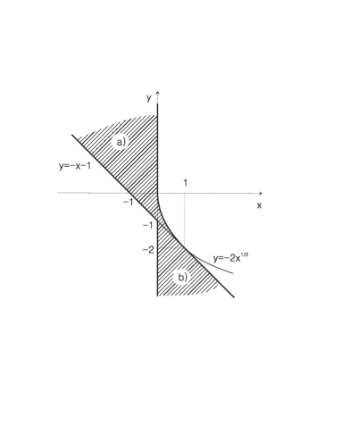
Figure 1: The region where stationary states of a positively ($\varphi^{\prime}>0$) charged ring may exist is crosshatched. $y=r^{2}\varphi^{\prime}H_{z}$, $x=1+r^{2}\varphi^{\prime}E_{r}$ and $\dot{\varphi}\geq 0$. The region $a)$, which is bounded from below by the straight line $y=-x-1$, corresponds to the situation when Eq. (26) is taken with sign $+$, and the region $b)$, which is bounded by the axis $y$ and the curve $y=-2x^{1/2}$, corresponds to the branch with sign $-$. In the overlap of regions $a)$ and $b)$ there may exist stationary states of the ring that have different angular velocities for the same values of the external field, charge, and ring radius.

The requirements that the radicand be nonnegative and that the velocity of the string be less than the velocity of light impose constraints on the fields $H_{z}$ and $E_{r}$, under which stable states of the ring may exist. These requirements are illustrated graphically in Fig. 1. For example, if there is no electric field and a ring of radius $r$ is uniformly charged, then the magnetic field can hold this ring only if

$$|H_{z}(r)|\geq\frac{|Q|}{\pi r^{2}},$$ (27)

where $Q$ is the total charge of the ring.

Equations (24) are rather complicated in the general case; therefore, we restrict the analysis to a uniformly charged ring ($\varphi^{\prime\prime}=0$) for $E_{r}=0$. Then, we have

$$\ddot{\varphi}=\frac{c^{2}\varphi^{\prime}}{2}E_{\varphi},\;\;\;\;\;\varphi^{\prime}=\frac{2\pi}{Q},\;\;\;\;\;\frac{r\dot{\varphi}}{c}=-\frac{\pi r^{2}H_{z}}{Q}-\sqrt{\frac{\pi^{2}r^{4}H_{z}^{2}}{Q^{2}}-1},$$ (28)

where we used the fact that the equality $\varphi^{\prime\prime}=0$ implies the equality $\dot{\varphi}^{\prime}=0$. The substitution of the expression for $\dot{\varphi}$ into the equation for $\ddot{\varphi}$ in (28) yields equations for the fields that admit such stationary configurations.

For example, in the nonrelativistic limit $r^{2}\dot{\varphi}^{2}\ll c^{2}$, we obtain the following solution to (28):

$$\frac{r\dot{\varphi}(t)}{c}=-\frac{Q}{2\pi r^{2}H_{z}(t)},\;\;\;\;\;\varphi^{\prime}(\sigma)=\frac{2\pi}{Q},\;\;\;\;\;2\pi^{2}r^{3}c^{2}E_{\varphi}(t)=Q^{2}\frac{\dot{H}_{z}(t)}{H_{z}^{2}(t)},$$ (29)

whereas, in the ultrarelativistic limit $r^{2}\dot{\varphi}^{2}\approx c^{2}$, Eqs. (28) lead to the equalities

$$\frac{r\dot{\varphi}(t)}{c}=-\frac{Q}{\pi r^{2}H_{z}(t)},\;\;\;\;\;\varphi^{\prime}(\sigma)=\frac{2\pi}{Q},\;\;\;\;\;\dot{H}_{z}(t)=-c\frac{E_{\varphi}(t)}{r}(1+\frac{\pi r^{2}}{Q}H_{z}(t)).$$ (30)

Thus, a uniformly charged ring does not change its radius only if the external fields satisfy Eqs. (28) (or Eqs. (29) and (30) in the nonrelativistic and ultrarelativistic cases, respectively), provided, of course, that $E_{r}=0$.

Now, we proceed to solving the dynamical equations (22). Consider the case when there are no external fields. The solution of the second equation in (22) yields

$$r(t)=\sqrt{\rho^{2}+c^{2}(t+\tau)^{2}},\;\;\;\;\;\rho=r(0)\sqrt{1-\frac{\dot{r}^{2}(0)}{c^{2}}},\;\;\;\;\;\tau=\frac{r(0)\dot{r}(0)}{c^{2}}.$$ (31)

Then, the first equation takes the form

$$\ddot{\varphi}-2\frac{\dot{\varphi}^{\prime}\dot{\varphi}}{\varphi^{\prime}}-\frac{\varphi^{\prime\prime}}{\varphi^{\prime 2}}(\frac{c^{2}\rho^{2}}{r^{4}}-\dot{\varphi}^{2})+2\frac{\dot{r}\dot{\varphi}}{r}=0,$$ (32)

whence

$$\frac{d}{dt}\int\limits_{0}^{Q}{d\sigma r^{2}\dot{\varphi}}=0.$$ (33)

If, in addition, we require that $\dot{\varphi}^{\prime}=0$, which physically means that all points of the ring rotate with the same velocity, then we obtain the solution

$$r^{2}(t)\dot{\varphi}(t)=r^{2}(0)\dot{\varphi}(0),\;\;\;\;\;\varphi^{\prime}(\sigma)=\frac{2\pi}{Q}.$$ (34)

As expected, the equation for $\varphi$ represents the angular momentum conservation law.

Solution (31) shows that, after a certain period of time, the ring will expand with a velocity close to the velocity of light; therefore, it is worthwhile to consider the ultrarelativistic limit of Eq. (32); i.e., it is worthwhile to require that $c^{2}-\dot{r}^{2}-r^{2}\dot{\varphi}^{2}\approx 0$. In this case, we have the following conservation law:

$$\frac{r^{2}(t)\dot{\varphi}(t,\sigma)}{\varphi^{\prime 2}(t,\sigma)}=\frac{r^{2}(0)\dot{\varphi}(0,\sigma)}{\varphi^{\prime 2}(0,\sigma)}.$$ (35)

This equation can be solved by the method of characteristics (see, for example, [16]). In a particular case when

$$\dot{\varphi}(0,\sigma)/\varphi^{\prime 2}(0,\sigma)=\lambda^{2}(0,\sigma)r^{2}(0)\dot{\varphi}(0,\sigma)=b=const,$$

i.e., when the linear density of the effective angular momentum is the same at all points of the string, we obtain

$$\begin{split}\dot{\varphi}(t,\sigma)&=\frac{br^{2}(0)}{r^{2}(t)}\varphi^{\prime 2}(0,\sigma_{0}(t,\sigma)),\\ \sigma&=\sigma_{0}(t,\sigma)-\frac{2br^{2}(0)}{\rho c}\left(\arctan{\frac{c(t+\tau)}{\rho}}-\arctan{\frac{c\tau}{\rho}}\right)\varphi^{\prime}(0,\sigma_{0}(t,\sigma)).\end{split}$$ (36)

The above equation should be considered as an equation for $\sigma_{0}(t,\sigma)$ for a certain prescribed $Q$-periodic function $\varphi^{\prime}(0,\sigma_{0})$ whose fundamental harmonic is equal to $2\pi Q^{-1}$.

To conclude this section, consider the effective dynamics of a charged ring all of whose points move with the same angular velocity ($\dot{\varphi}^{\prime}=0$) in a uniform magnetic field $H_{z}=const$. In this case, from (22) and (23) we obtain the system of equations

$$\frac{(c^{2}-\dot{r}^{2}+r^{2}\dot{\varphi}^{2})(c^{2}-\dot{r}^{2}-r\ddot{r})}{r^{2}\varphi^{\prime}(c^{2}-\dot{r}^{2})^{3/2}}=-r\dot{\varphi}H_{z},\;\;\;\;\;\frac{r\dot{\varphi}}{\sqrt{c^{2}-\dot{r}^{2}}}+\frac{\pi H_{z}}{2Q}r^{2}=M,$$ (37)

where $M$ is a certain constant defined by the initial data. The first equation implies, in particular, that $\varphi^{\prime}=2\pi Q^{-1}$. Substituting the expression for $r\dot{\varphi}$ from the second equation into the first, we obtain an equation for the function $r(t)$ alone, which has the form

$$\sqrt{c^{2}-\upsilon^{2}}=k(1+(M-(\pi H_{z}/2Q)r^{2})^{2})/r,$$ (38)

where $\upsilon(r(t))\equiv\dot{r}(t)$ and $k$ is an integration constant. Let us express the equations of motion in dimensionless variables. Introduce $r_{0}=|\pi H_{z}/2Q|^{-1/2}$ and redefine $r$ and $t$ as $r\rightarrow r_{0}r$ and $t\rightarrow t\,r_{0}/c$. For example, the velocity in these coordinates is measured in the units of the velocity of light. Then, the equations of motion of a charged ring are expressed as

$$\frac{\upsilon^{2}}{2}+\frac{1}{2}\left[k^{2}\frac{(1+L^{2})^{2}}{r^{2}}-1\right]=0,\;\;\;\;\;\dot{\varphi}=k\frac{L(1+L^{2})}{r^{2}},$$ (39)

where $L=M-\operatorname{sgn}{(H_{z}/Q)}r^{2}$.

Figure 2: The functions of the potential $U(r)$ (heavy line) and the angular velocity $r\dot{\varphi}$ (thin line). The diagrams correspond to the initial data $r(0)\approx 1.844$, $\upsilon(0)=0.1$, $M=3$ and $\operatorname{sgn}{(H_{z}/Q)}=1$. The potential attains its minimum at the point $r_{ext}\approx 1.755$.

The first equation in (39) resembles the equation of motion of a particle of unit mass with zero total energy in the potential field $U(r)=\left[k^{2}r^{-2}(1+L^{2})^{2}-1\right]/2$ the only difference between these equations is that the form of $U(r)$ depends on the initial data $r(0)$, $\upsilon(0)$ and $\dot{\varphi}(0)$ (see Fig. 2). The potential has a single extremum at the point

$$r_{ext}^{2}=\frac{1}{3}(\operatorname{sgn}{(\frac{H_{z}}{Q})}M+\sqrt{4M^{2}+3}),$$ (40)

and indefinitely increases as $r\rightarrow 0$ and $r\rightarrow+\infty$ ; therefore, for any initial data, the system will oscillate about the equilibrium point $r_{ext}$. Note that the minimal value of $r_{ext}$ is equal to $\sqrt{2}/2$, which agrees with the results of the previous analysis of the stationary states (27) of a charged ring.

We can evaluate the ratio of the oscillation frequency $\omega$ of the charged ring in the neighborhood of the equilibrium point $r_{ext}$ to the mean angular frequency $\omega_{0}$ of its rotation. In the harmonic approximation, the first frequency is defined by $U^{\prime\prime}(r_{ext})$, and the second, by $|\dot{\varphi}(r_{ext})|$; hence, we have

$$\frac{\omega}{\omega_{0}}\approx\frac{1}{r}\frac{(4r^{2}-\sqrt{4r^{4}-1})^{1/2}}{(2r^{2}-\sqrt{4r^{4}-1})^{3/2}},$$ (41)

where $r=r_{ext}$. This ratio uniformly increases from $2$ to infinity as $r_{ext}$ increases; for large values of $r_{ext}$ it increases as $8\sqrt{2}r_{ext}^{3}$. For example, a threefold increase in the linear dimensions of a synchrotron leads to a ninefold increase in the oscillation frequency for the same mean angular velocities of the high-current beam of particles, other characteristics, such as $H_{z}$, $Q$ and $\chi$, remaining constant.

Thus, an absolutely elastic uniformly charged ring in a uniform magnetic field oscillates about the equilibrium point $r_{ext}$, $\dot{\varphi}_{ext}$, according to Eqs. (39) with frequency $\omega$; the ratio of this frequency to the angular frequency of the ring is defined by (41). Therefore, we can expect that, when the energy inflow compensates the energy losses, a high-current beam of charged particles in a synchrotron will also produce radiation at this frequency, in addition to the well-known synchrotron radiation. For example, if one could separate these two types of radiation by certain characteristics and measure the ratio $\omega/\omega_{0}$, then one would determine the equilibrium position $r_{ext}$ in the units of $r_{0}$ by formula (41).

Among the disadvantages of the model of an absolutely elastic charged string as applied to the description of a high-current beam of charged particles is the fact that this model does not take into account the radiation reaction due to the synchrotron radiation, which becomes significant at large angular velocities.

4 An absolutely nonstretchable string

In this section, we consider the dynamics of a thin, absolutely nonstretchable charged string with a current with regard to the first-order correction due to the self-action. We derive equations of motion for such a string, investigate its stationary states in the absence of an external electromagnetic field, and find a class of solutions to the equations of motion for a uncharged string with a current and for a uniformly charged string.

Suppose given a closed string $N$ with coordinates $\{\tau,\sigma\}$, $\sigma\in[0,L)$, that is embedded into the Minkowski space $\mathbb{R}^{3,1}$ by a smooth mapping $x(\tau)$. In relativistic mechanics, the concept of nonstretchability makes sense only in a certain distinguished frame of reference. Let us introduce a $4$-vector $n^{\mu}$, $n^{2}=1$, that characterizes such a frame of reference; then, the action that describes the free dynamics of an absolutely nonstretchable string is given by

$$S_{0}[x,\varkappa,\kappa^{0},\kappa^{1}]=\int\limits_{N}{d\tau d\sigma\left(\varkappa(h_{00}+h)+\kappa^{0}(n^{\mu}\dot{x}_{\mu}-c)+\kappa^{1}n^{\mu}x^{\prime}_{\mu}\right)},$$ (42)

where $\varkappa$, $\kappa^{0}$ and $\kappa^{1}$ are Lagrange multipliers of the constraints that guarantee the nonstretchability of the string. It is obvious that action (42) is not invariant under the change of coordinates $\{\tau,\sigma\}$, hence, there are no constraints (9) on the form of the linear density of charge and the current in this case.

The effective equations of motion (7) or a thin absolutely nonstretchable charged string with a current in the distinguished frame of reference $n^{\mu}=(1,0,0,0)$ are expressed as

$$\begin{split}-&\partial_{i}(L^{ij}\partial_{j}x_{\mu}+\kappa^{i}\delta^{0}_{\mu})=\frac{1}{c}F_{\mu\nu}e^{i}\partial_{i}x^{\nu},\;\;\;\;\;L^{ij}\equiv\frac{\chi}{c}\frac{h_{kl}e^{k}e^{l}h^{ij}-2e^{i}e^{j}}{\sqrt{|h|}}+2\varkappa(\delta^{i}_{0}\delta^{j}_{0}+hh^{ij}),\\ h&{}_{00}=-h,\;\;\;\;\;\dot{x}^{0}=c,\;\;\;\;\;x^{\prime 0}=0.\end{split}$$ (43)

The last three equations in (43) represent the condition of “relativistic nonstretchability”. Indeed, the equation $h_{00}=-h$ has the form

$$\mathbf{x}^{\prime 2}=1-\frac{(\dot{\mathbf{x}}\mathbf{x}^{\prime})^{2}}{c^{2}-\dot{\mathbf{x}}^{2}},$$ (44)

which immediately implies that the coordinate $\sigma$ is a natural parameter on the string with a correction for relativistic contraction. Since $\sigma$ ranges from $0$ to $L$, the fulfillment of equality (44) at any point of the string automatically implies that the string of length $L$ is nonstretchable.

Since we consider a closed string, all functions entering Eq. (43) must be periodic in $\sigma$. For an open string with free ends, the periodicity condition is replaced by the equality

$$L^{1i}\partial_{i}x_{\mu}+\kappa^{1}\delta^{0}_{\mu}=0,$$ (45)

at the ends of the string.

We will consider the effective dynamics of a closed string in the absence of external electromagnetic fields. The unknown fields $\kappa^{i}$ can be obtained from the first two equations in (43) by setting $\mu=0$. As a result, we are left with four equations for four unknown functions $\mathbf{x}(t,\sigma)$ and $\varkappa(t,\sigma)$:

$$L^{ij}\partial_{ij}\mathbf{x}+\partial_{i}L^{ij}\partial_{j}\mathbf{x}=0,\;\;\;\;\;\mathbf{x}^{\prime 2}=1-\frac{(\dot{\mathbf{x}}\mathbf{x}^{\prime})^{2}}{c^{2}-\dot{\mathbf{x}}^{2}}.$$ (46)

The consistency condition for this system yields an equation for $\varkappa(t,\sigma)$. The physical meaning of the field $\varkappa(t,\sigma)$ is that it compensates for the forces that stretch (contract) the string.

Let us find the stationary configurations of the string that are consistent with Eqs. (46), i.e. set $\dot{\mathbf{x}}\equiv 0$ in the equations of motion. We can easily show that, in this case, the equations of motion are reduced to the system

$$2\varkappa^{\prime}+\frac{(\lambda^{2})^{\prime}}{c}+2\frac{\lambda\dot{I}}{c^{3}}=0,\;\;\;\;\;2\varkappa+\frac{\lambda^{2}}{c}+\frac{I^{2}}{c^{3}}=0,\;\;\;\;\;\mathbf{x}^{\prime 2}=1.$$ (47)

Taking into account the charge conservation law, $\dot{\lambda}+I^{\prime}=0$, we have

$$\varkappa=-\frac{c^{2}\lambda^{2}+I^{2}}{2c^{3}},\;\;\;\;\;\dot{(\lambda I)}=0,\;\;\;\;\;\mathbf{x}^{\prime 2}=1.$$ (48)

Thus, if the product of the charge density multiplied by the current is independent of time and all points of the string are at rest at the initial moment, then there exists $\varkappa(t,\sigma)$ such that the string retains its initial configuration. The question concerning the stability of such solutions remains open.

Next, consider the nonrelativistic dynamics of a string described by Eqs. (46) in the absence of the current, $I=0$ (charged dielectric), as well as for $\lambda=0$ (uncharged conductor). The nonrelativistic limit is understood in the following sense. Let $l$ be a characteristic scale of variation of the field $\mathbf{x}(t,\sigma)$, for example, the length of the string; then, we formally define the order of smallness as follows:

$$[\dot{\mathbf{x}}/c]\ll 1,\;\;\;\;\;[l^{k}\partial^{k+1}_{\sigma}\mathbf{x}]=[l\dot{\mathbf{x}}^{\prime}/c]=[l\ddot{\mathbf{x}}/c^{2}]=1.$$ (49)

In this case, the order of smallness of $\varkappa$ is determined from Eqs. (46).

For a charged dielectric, when $I=0$ and $\dot{\lambda}=0$, we obtain the following system of equations from (46) in the nonrelativistic limit:

$$\frac{\lambda^{2}}{c^{2}}\ddot{\mathbf{x}}+\Lambda\mathbf{x}^{\prime\prime}+\left[\Lambda^{\prime}+\frac{\ddot{\mathbf{x}}\mathbf{x}^{\prime}}{c^{2}}\Lambda\right]\mathbf{x}^{\prime}=0,\;\;\;\;\;\mathbf{x}^{\prime 2}=1,$$ (50)

where $\Lambda=2c\varkappa+\lambda^{2}$. Note that these equations are invariant under the Galilean transformations. Equations (50) can be resolved for the higher derivative only if $\Lambda\neq-\lambda^{2}$. In this case, we have

$$\frac{\lambda^{2}}{c^{2}}\ddot{\mathbf{x}}+\Lambda\mathbf{x}^{\prime\prime}+\frac{\lambda^{2}\Lambda^{\prime}}{\lambda^{2}+\Lambda}\mathbf{x}^{\prime}=0,\;\;\;\;\;\mathbf{x}^{\prime 2}=1.$$ (51)

The consistency condition for system (51) leads to the following equation for $\Lambda(t,\sigma)$

$$\left(\frac{\Lambda^{\prime}}{\lambda^{2}+\Lambda}\right)^{\prime}-\frac{\Lambda\mathbf{x}^{\prime\prime 2}}{\lambda^{2}}-\frac{\dot{\mathbf{x}}^{\prime 2}}{c^{2}}=0.$$ (52)

Thus, fixing $\Lambda(t,0)$ and $\Lambda^{\prime}(t,0)$, as well as $\mathbf{x}(0,\sigma)$ and $\dot{\mathbf{x}}(0,\sigma)$, subject to the conditions $\mathbf{x}^{\prime}(0,\sigma)\mathbf{x}^{\prime}(0,\sigma)=1$ and $\dot{\mathbf{x}}^{\prime}(0,\sigma)\mathbf{x}^{\prime}(0,\sigma)=0$, we can construct a unique solution $\mathbf{x}(t,\sigma)$ that satisfies Eqs. (51). Recall that all the functions must be $L$-periodic in the variable $\sigma$. This condition imposes constraints on the boundary conditions for the function $\Lambda(t,\sigma)$.

One can draw an instantaneous phase portrait for Eq. (52) (see Fig. 3). In particular, this portrait shows that, if $\Lambda(t,0)\neq-\lambda^{2}$, then $\Lambda(t,\sigma)\neq-\lambda^{2}$, $\forall\sigma\in[0,L)$, i.e. the quantity $(1+\Lambda/\lambda^{2})$ does not change its sign.

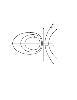
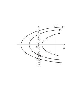
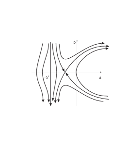
Figure 3: The instantaneous phase portrait for Eq. (52), here $p=\Lambda^{\prime}/(\lambda^{2}+\Lambda)$. The circles indicate the singular points of the vector field. At the left $\dot{\mathbf{x}}^{\prime 2}/c^{2}>\mathbf{x}^{\prime\prime 2}$(this case can be referred to as the case of small curvature of the string), at the middle $\dot{\mathbf{x}}^{\prime 2}/c^{2}=\mathbf{x}^{\prime\prime 2}$, and at the right $\dot{\mathbf{x}}^{\prime 2}/c^{2}<\mathbf{x}^{\prime\prime 2}$.

For a uniformly charged string, $\lambda=const$, Eqs. (51) and (52) are rewritten as

$$\frac{\ddot{\mathbf{x}}}{c^{2}}-(1-\operatorname{sgn}{(1+\frac{\Lambda}{\lambda^{2}})}e^{\Theta})\mathbf{x}^{\prime\prime}+\Theta^{\prime}\mathbf{x}^{\prime}=0,\;\;\;\;\;\Theta^{\prime\prime}+(1-\operatorname{sgn}{(1+\frac{\Lambda}{\lambda^{2}})}e^{\Theta})\mathbf{x}^{\prime\prime 2}-\frac{\dot{\mathbf{x}}^{\prime 2}}{c^{2}}=0,$$ (53)

where $\Theta=\ln{|1+\Lambda/\lambda^{2}|}$.

Using similar arguments for an uncharged conductor with a current, $\lambda=0$ and $I^{\prime}=0$, we obtain the following equations for $\varkappa\neq 0$ (this condition is an analogue of the inequality $\Lambda\neq-\lambda^{2}$, which arises in the case of a charged dielectric)

$$\frac{\ddot{\mathbf{x}}}{c^{2}}+(1+\operatorname{sgn}{(\varkappa)}e^{\Theta})\mathbf{x}^{\prime\prime}+\Theta^{\prime}\mathbf{x}^{\prime}=0,\;\;\;\;\;\Theta^{\prime\prime}-(1+\operatorname{sgn}{(\varkappa)}e^{\Theta})\mathbf{x}^{\prime\prime 2}-\frac{\dot{\mathbf{x}}^{\prime 2}}{c^{2}}=0,$$ (54)

where $\Theta=\ln{|2c^{3}\varkappa/I^{2}|}$. The instantaneous phase portrait for the second equation in (54) has always the same form (with obvious redefinitions) as the instantaneous phase portrait in the case of a weakly curved charged dielectric (Fig. 3 at the left). Therefore, periodic (in $\sigma$) solutions to the second equation in (54) may only exist when $\varkappa(t,0)<0$.

Let us find certain particular solutions to the equations obtained. Setting $\Theta^{\prime}(t,\sigma)=0$ in Eqs. (53) or (54), we obtain the system

$$\ddot{\mathbf{x}}-u^{2}(t)\mathbf{x}^{\prime\prime}=0,\;\;\;\;\;\dot{\mathbf{x}}^{\prime 2}=u^{2}(t)\mathbf{x}^{\prime\prime 2},\;\;\;\;\;\mathbf{x}^{\prime 2}=1.$$ (55)

In this case, the dynamics of a uniformly charged dielectric and an uncharged conductor are described by the same system of equations. Let us simplify the situation by assuming that $u(t)=const$. Then, there exists a class of solutions of the form

$$\mathbf{x}(t,\sigma)=\mathbf{V}t+\mathbf{x}_{0}(\sigma+ut),$$ (56)

where $\mathbf{V}$ is a certain constant vector and $\mathbf{x}_{0}(\sigma)$, $\mathbf{x}_{0}^{\prime 2}=1$ defines the initial configuration of the string. Substituting the general solution of the wave equation into the remaining two equations, one can show that (56) provides the only possible solutions to Eqs. (55) for $u=const$. Solutions describe a string that “flows” along itself with the velocity $u$.

5 Concluding remarks

We have investigated the effective dynamics of a thin electrically charged string with a current with regard to the leading contribution of the self-action. This approximation has allowed us to describe the effective dynamics of a string in an external electromagnetic field in the form of second-order partial differential equations and obtain their exact solutions for certain simple models of a string in the electromagnetic field of a special form.

We have not analyzed the question concerning the stability of the solutions obtained. This problem may become one of possible directions of further investigations. Another direction of research may be the study of radiation characteristics of an absolutely elastic charged ring (a high-current beam of charged particles) in an external uniform magnetic field; the existence of such a radiation was discussed at the end of Section 3. Moreover, it would be interesting to find other solutions to the effective equations of motion of a string or to carry out a numerical analysis of these equations.

References

- [1] H.A. Lorentz, Theory of electrons, B.G. Teubner, Leipzig (1909).
- [2] P.A.M. Dirac, Proc. Roy. Soc. London A 167, 148 (1938).
- [3] B.S. DeWitt, R.W. Brehme, Ann. Phys. 9, 220 (1960).
- [4] A.O. Barut, N. Unal, Phys. Rev. A 40, 5404 (1989).
- [5] P.E.G. Rowe, G.T. Rowe, Phys. Rep. 149, 287 (1987).
- [6] B.P. Kosyakov, Teor. Mat. Fiz. 119, 119 (1999) (in Russian); Theor. Math. Phys. 119, 493 (1999). hep-th/0207217.
- [7] P.O. Kazinski, S.L. Lyakhovich, and A.A. Sharapov, Phys. Rev. D 66, 025017 (2002). hep-th/0201046.
- [8] P.O. Kazinski and A.A. Sharapov, Class. Quantum Grav. 20, 2715 (2003). hep-th/0212286.
- [9] B. Carter, Phys. Lett. B 404, 246 (1997). hep-th/9704210.
- [10] A.O. Barut and P.A. Pavšič, Phys. Lett. B 331, 45 (1994).
- [11] J. Isberg, U. Lindström, B. Sundborg, and G. Theodoridis, Nucl. Phys. B 411, 122 (1994). hep-th/9307108.
- [12] M.B. Hindmarsh and T.W.B. Kibble, Rept. Prog. Phys. 58, 477 (1995). hep-ph/9411342.
- [13] P.O. Kazinski and A.A. Sharapov, Teor. Mat. Fiz. 143, 375 (2005) (in Russian); Theor. Math. Phys. 143, 798 (2005).
- [14] E. Witten, Nucl. Phys. B 249, 557 (1985).
- [15] A. Buonanno and T. Damour, Phys. Lett. B 432, 51 (1998). hep-th/9803025.
- [16] V.I. Arnold, Geometric methods in the theory of ordinary differential equations, Springer-Verlag, New York, (1983).
- [17] D.R. Merkin, Introduction to mechanics of a flexible thread, Nauka, Moscow, (1980) (in Russian).