Plate with a hole obeys the averaged null energy condition

Abstract

The negative energy density of Casimir systems appears to violate general relativity energy conditions. However, one cannot test the averaged null energy condition (ANEC) using standard calculations for perfectly reflecting plates, because the null geodesic would have to pass through the plates, where the calculation breaks down. To avoid this problem, we compute the contribution to ANEC for a geodesic that passes through a hole in a single plate. We consider both Dirichlet and Neumann boundary conditions in two and three space dimensions. We use a Babinet’s principle argument to reduce the problem to a complementary finite disk correction to the perfect mirror result, which we then compute using scattering theory in elliptical and spheroidal coordinates. In the Dirichlet case, we find that the positive correction due to the hole overwhelms the negative contribution of the infinite plate. In the Neumann case, where the infinite plate gives a positive contribution, the hole contribution is smaller in magnitude, so again ANEC is obeyed. These results can be extended to the case of two plates in the limits of large and small hole radii. This system thus provides another example of a situation where ANEC turns out to be obeyed when one might expect it to be violated.

I Introduction

The standard Casimir calculation of the energy density between a pair of parallel plates (see for example Mostepanenko and Trunov (1997)) yields a negative energy density between the plates. While this result poses no problem in the calculation of the usual Casimir force, it presents a puzzle for general relativity. One can construct a spacetime with an arbitrary geometry $R_{\lambda\nu}$ simply by constructing the energy-momentum tensor to solve Einstein’s equations

$$T_{\lambda\nu}=\frac{1}{8\pi G}\left(R_{\lambda\nu}-\frac{1}{2}g_{\lambda\nu}R\right)\,.$$ (1)

The only way to prevent the appearance of exotic phenomena, such as closed timelike curves Hawking (1992), traversable wormholes Morris et al. (1988), or superluminal travel Olum (1998), is to place restrictions on the allowed energy-momentum tensors $T_{\lambda\nu}$. While these conditions are all obeyed in classical physics, the negative energy density of the quantum Casimir system violates most such conditions, including the weak energy condition (WEC) and the null energy condition (NEC), which require that $T_{\lambda\nu}V^{\lambda}V^{\nu}\geq 0$ for timelike and null vectors respectively. A still weaker condition, which is still strong enough to rule out exotic phenomena (and to prove singularity theorems Penrose (1965); Galloway (1981); Roman (1986, 1988)), is that the null energy condition hold only when averaged over a complete geodesic (ANEC). Geodesics parallel to the plates obey NEC, so any candidate for ANEC violation would need to pass through the plates themselves. Therefore one cannot test ANEC using the standard Casimir calculation in which one imposes ideal boundary conditions, since this calculation is not valid within each plate. One approach to resolve this question is to model the plate using a domain wall background Graham and Olum (2003); Olum and Graham (2003); in this case the effect of the domain wall modifies the calculation significantly, so that ANEC is obeyed. In a number of other examples in which one might expect to find that ANEC is violated, explicit calculation shows that it is obeyed Schwartz-Perlov and Olum (2003); Graham et al. (2004). Other calculations also show that energy condition violation is more difficult to achieve in realistic situations than idealized models would suggest Sopova and Ford (2002, 2005). ANEC is also known to be obeyed by free scalar Klinkhammer (1991) and electromagnetic Folacci (1992) fields in flat spacetime. Other works have found restrictions on energy condition violation in flat space Borde et al. (2002); Ford and Roman (1995, 1996).

In this paper we consider an alternative modification to the Casimir problem that one might expect would allow the NEC violation between the plates to extend to ANEC violation: we imagine a plate with a small hole, through which the geodesic can pass without encountering the material of the plate. Our primary calculation is for the case of a single Dirichlet plate, which also leads to a negative energy density for minimal coupling. We consider both two and three spatial dimensions. We also give extensions of this result to Neumann boundaries and to the case of two plates in extreme limits.

II Null Energy Condition Outside a Boundary

Since our geodesic never passes through the material that actually imposes the boundary, we need only consider the quantum field $\phi$ in empty space. The effect of the boundary will be to modify the normal mode expansion for $\phi$. We will then integrate $V^{\lambda}V^{\nu}T_{\lambda\nu}$, where $T_{\lambda\nu}$ is the stress-energy tensor, over the null geodesic $V^{\lambda}$ perpendicular to the plate, passing through the center of the hole. The stress-energy tensor for a minimally-coupled scalar field is

$$T_{\lambda\nu}=\partial_{\lambda}\phi\partial_{\nu}\phi-\frac{1}{2}\eta_{\lambda\nu}\left[\partial^{\lambda}\phi\partial_{\lambda}\phi\right]\,.$$ (2)

For a null vector, $\eta_{\lambda\nu}V^{\lambda}V^{\nu}=0$, so we have

$$T_{\lambda\nu}V^{\lambda}V^{\nu}=\left(V^{\alpha}\partial_{\alpha}\phi\right)^{2}\,.$$ (3)

For a static system, $T_{0i}=0$ for $i=1,2,3$. If we further choose spatial coordinates in which $T_{ij}$ is diagonal and $V=(1,{\bf v})$, then

$$T_{\lambda\nu}V^{\lambda}V^{\nu}=\dot{\phi}^{2}+\sum_{i}\left(v_{i}\partial_{i}\phi\right)^{2}\,.$$ (4)

Let the center of the hole lie at the origin and let the $z$ axis be the direction perpendicular to the plate, along which the geodesic lies. For that path,

$$T_{\lambda\nu}V^{\lambda}V^{\nu}=\dot{\phi}^{2}+\left(\partial_{z}\phi\right)^{2}\,.$$ (5)

III Babinet’s Principle

It will greatly simplify the scattering theory techniques we would like to use in our Casimir calculation Bordag and Lindig (1996); Saharian (2001); Graham et al. (2002) to be able to consider a boundary condition in a local region. Therefore we apply a Babinet’s principle argument to reexpress the result for a plate with a hole in terms of the results when the boundary condition is applied to an entire plate and when a complementary boundary condition is applied to a disk. The former is well-known, while the latter can be computed using scattering theory in elliptical or spheroidal coordinates.

We start in empty space, and write the field there in terms of normal modes that are even or odd in the coordinate across the boundary. Next we consider a perfectly reflecting Dirichlet boundary with no holes. The free-space odd modes obey the boundary conditions, but the even modes do not. Instead, we have new even modes, which are just the odd mode on the right and minus the odd mode on the left, as shown in Fig. 1.

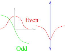
Figure 1: In free space (left) we have even and odd normal mode wave functions. In the presence of a Dirichlet plate (right), the even functions are replaced by the odd functions with a change of sign crossing the plate.

If we let $E$ denote a sum over the free-space even modes and $O$ the same sum over the odd modes, then in free space we have $E+O$, whereas with the barrier we have $O+O$. Therefore, the renormalized energy, the difference between the energy with the barrier and the energy in free space, is $O-E$. If we have Neumann conditions instead, the situation is precisely reversed and the energy is $E-O$.

Now we consider the Dirichlet plate with holes of arbitrary shapes. Once again the odd modes are unaffected, and we have new even modes that vanish on the barrier but are continuous in the holes, as shown in Fig. 2.

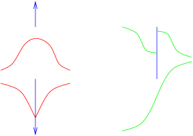
Figure 2: If there is a hole in the Dirichlet plate (left), the new even functions satisfy Neumann conditions in the hole and Dirichlet conditions elsewhere. The odd functions for a patch with the same shape as the hole (right) are the same except for a change of sign between sides.

Since they are even, they satisfy Neumann conditions in the hole. Let us call the contribution of those modes $A$. The energy with the perforated barrier is thus $A+O$, so the renormalized energy is $A-E$.

Finally, suppose that there are Neumann patches where the holes were. The even modes are unaffected, but there are new odd modes. In order to be odd and continuous they must satisfy Dirichlet conditions on the plane outside the patches. Thus, except for a change of sign on one side, these are the exact same modes of the previous paragraph, as shown in Fig. 2. Therefore the total energy is $A+E$ and the renormalized energy is $A-O$. Thus we conclude that

$$\hbox{[Dirichlet plate w/hole]}-\hbox{[Complementary Neumann disk]}=\hbox{[Entire Dirichlet plane]}$$ (6)

and similarly

$$\hbox{[Neumann plate w/hole]}-\hbox{[Complementary Dirichlet disk]}=\hbox{[Entire Neumann plane]}.$$ (7)

IV Line Segment in Two Spatial dimensions

In this section we consider a scalar field in 2+1 dimensions with boundary conditions imposed on a line segment from $x=-d$ to $x=d$. In circular coordinates, we can decompose a free, real, massless scalar field in modes as

$$\phi(r,\theta)=\sum_{m=0}^{\infty}{}^{\prime}\int_{0}^{\infty}dk\,\sqrt{\frac{k}{2\pi\omega}}J_{m}(kr)\left(\cos m\theta\,b_{k}^{m}{}^{\dagger}+\sin m\theta\,c_{k}^{m}{}^{\dagger}\right)e^{i\omega t}+\text{c.c.}$$ (8)

where the prime on the summation sign indicates that for $m=0$, there is no sin mode and instead of $\cos 0=1$ we have $1/\sqrt{2}$.

Now we go to elliptical coordinates. For notational consistency with the three-dimensional case, we consider the $x$-$z$ plane. The foci will be located at $x=\pm d$, and the the geodesic will run along the $z$ axis. Elliptical coordinates $\mu$, $\theta$ are given by

$$x = d\cosh\mu\cos\theta$$ (9)

$$z = d\sinh\mu\sin\theta$$ (10)

so

$$r=\sqrt{x^{2}+z^{2}}=d\sqrt{\frac{\cosh 2\mu+\cos 2\theta}{2}}\to\frac{d}{2}e^{\mu}$$ (11)

as $\mu\to\infty$.

We define our Mathieu functions following the conventions of Abramowitz and Stegun Abramowitz and Stegun (1972) but extending their notation to be more similar to that of Bessel functions. The angular functions are $ce_{m}(\theta,q)$ and $se_{m}(\theta,q)$. They satisfy

$$y^{\prime\prime}+(a-2q\cos 2\theta)y=0$$ (12)

where $q=(dk/2)^{2}$, and are normalized so that

$$\int_{0}^{2\pi}d\theta ce_{m}(\theta,q)^{2}=\int_{0}^{2\pi}d\theta se_{m}(\theta,q)^{2}=\pi\,.$$ (13)

This normalization holds even for $ce_{0}$, but there is no such function as $se_{0}$. Thus the normalization is precisely the same as the circular functions used above, including the special case for $m=0$.

The radial functions of the first kind are $Je_{m}(\mu,q)$ and $Jo_{m}(\mu,q)$ and are precisely the functions called $Mc_{m}^{(1)}(\mu,q)$ and $Ms_{m}^{(1)}(\mu,q)$ respectively in Abramowitz and Stegun (1972). They satisfy

$$y^{\prime\prime}-(a-2q\cosh 2\mu)y=0$$ (14)

and go asymptotically to $J_{m}(\sqrt{q}e^{\mu})=J_{m}(kr)$. Note that the functions $Je_{m}$ and $Jo_{m}$ defined in Morse and Feshbach (1953) have an additional factor of $\sqrt{\pi/2}$. Analogously, we denote the radial functions of the second kind as $Ye_{m}(\mu,q)$ and $Yo_{m}(\mu,q)$, which are $Mc_{m}^{(2)}(\mu,q)$ and $Ms_{m}^{(2)}(\mu,q)$ in Abramowitz and Stegun (1972).

The normalization of radial functions depends only on their asymptotics, so $Je_{m}$ and $Jo_{m}$ have the same normalization as $J_{m}$. Thus the field becomes

$$\phi(\mu,\theta)=\sum_{m=0}^{\infty}{}^{\prime}\int_{0}^{\infty}dk\,\sqrt{\frac{k}{2\pi\omega}}\left(Je_{m}(\mu,q)ce_{m}(\theta,q)b_{k}^{m}{}^{\dagger}+Jo_{m}(\mu,q)se_{m}(\theta,q)c_{k}^{m}{}^{\dagger}\right)e^{i\omega t}+\text{c.c.}$$ (15)

where the prime on the summation sign indicates that the second term is included only for $m>0$.

Now we consider Neumann conditions along the line segment, which is $\mu=0$. The even wavefunctions obey the conditions already, because $dJe_{m}/d\mu=0$ at $\mu=0$, but the odd functions need to be modified. Instead of $\psi o^{m}_{k}=0$ we need $d\psi o^{m}_{k}/d\mu=0$. For the free case we had

$$Jo_{m}(\mu,q)=\frac{1}{2}\left[Ho^{(1)}_{m}(\mu,q)+Ho^{(2)}_{m}(\mu,q)\right]$$ (16)

where $Ho^{(1)}=Jo_{m}+iYo_{m}$ is the function called $Ms_{m}^{(3)}$ in Abramowitz and Stegun (1972) and $Ho^{(2)}_{m}=Jo_{m}-iYo_{m}$ is $Ms_{m}^{(4)}$. Now we need

$$\psi o_{m}(\mu,q)=\frac{1}{2}\left[e^{2i\delta}Ho^{(1)}_{m}(\mu,q)+Ho^{(2)}_{m}(\mu,q)\right]$$ (17)

where

$$e^{2i\delta}=-\frac{Ho^{(2)}_{m}{}^{\prime}(0,q)}{Ho^{(1)}_{m}{}^{\prime}(0,q)}$$ (18)

and the derivative is with respect to $\mu$.

We can then compute the renormalized vacuum expectation value of the time-derivative term in Eq. (5),

$$\langle\dot{\phi}^{2}\rangle = \frac{1}{2\pi}\sum_{m=1}^{\infty}\int_{0}^{\infty}dk\,k\omega\left(|\psi o_{m}(\mu,q)|^{2}-Jo_{m}(\mu,q)^{2}\right)se_{m}(\mu,q)^{2}$$ (19)

and we can write

$$|\psi o_{m}(\mu,q)|^{2}-Jo_{m}(\mu,q)^{2}=\frac{1}{4}\left[\left(e^{2i\delta}-1\right)Ho^{(1)}_{m}(\mu,q)^{2}+\left(e^{-2i\delta}-1\right)Ho^{(2)}_{m}(\mu,q)^{2}\right]\,.$$ (20)

We want to extend the range of integration to include negative $k$. The term $se_{m}(\mu,q)^{2}$ is unchanged by going to negative $k$, while $Jo$ and $Ho$ behave just like the corresponding Bessel functions. Thus the situation is exactly as in the circular case Saharian (2001); Schwartz-Perlov and Olum (2003): extending the range of integration exchanges the two terms in Eq. (20), so we can consider only the first term integrated over the entire real axis. When we close the contour at infinity, we get the contribution from the branch cut in $\omega=\sqrt{k}$. With $k=i\kappa$, the angular function becomes $se_{m}(\theta,-q)$, and the radial functions have the same continuation as Bessel functions,

$$Jo_{m}(\mu,-q) = i^{m}Io_{m}(\mu,q)$$ (21)

$$Ho^{(1)}_{m}(\mu,-q) = \frac{2}{\pi}i^{-(m+1)}Ko_{m}(\mu,q)$$ (22)

where $Io_{m}$ and $Ko_{m}$ are exactly as in Abramowitz and Stegun (1972). Thus

$$e^{2i\delta_{m}(i\kappa)}-1=(-)^{m+1}i\pi\frac{Io_{m}^{\prime}(0,\varphi)}{Ko_{m}^{\prime}(0,\varphi)}$$ (23)

where $\varphi=(d\kappa/2)^{2}=-q.$

Putting it all together we have

$$\langle\dot{\phi}^{2}\rangle = \frac{(-)^{m}i}{\pi^{3}}\sum_{m=1}^{\infty}\int_{0}^{\infty}d\kappa\left(e^{2i\delta}-1\right)\kappa^{2}Ko_{m}(\mu,\varphi)^{2}se_{m}(\theta,-\varphi)^{2}$$ (24)

$$= \frac{1}{\pi^{2}}\sum_{m=1}^{\infty}\int_{0}^{\infty}d\kappa\frac{Io_{m}^{\prime}(0,\varphi)}{Ko_{m}^{\prime}(0,\varphi)}\kappa^{2}Ko_{m}(\mu,\varphi)^{2}se_{m}(\theta,-\varphi)^{2}\,.$$ (25)

On the axis, terms with $m$ even vanish, so we have

$$\langle\dot{\phi}^{2}\rangle=\frac{1}{\pi^{2}}\sum_{m=1}^{\infty}{}^{\prime}\int_{0}^{\infty}d\kappa\frac{Io_{m}^{\prime}(0,\varphi)}{Ko_{m}^{\prime}(0,\varphi)}\kappa^{2}Ko_{m}(\mu,\varphi)^{2}se_{m}(\pi/2,-\varphi)^{2}$$ (26)

where the prime on the summation sign indicates that we sum over odd values of $m$.

The other vacuum expectation value that we need is $\langle(\partial_{z}\phi)^{2}\rangle$. On the $z$ axis, $\partial_{z}\phi$ is just the component of the gradient in the $\mu$ direction, which differs from $\partial_{\mu}\phi$ by the inverse of the metric coefficient

$$h=d\sqrt{\cosh^{2}\mu-\cos^{2}\theta}=d\sqrt{\frac{\cosh 2\mu-\cos 2\theta}{2}}\,.$$ (27)

The calculation is otherwise similar. Instead of two powers of $\omega$ from time differentiation we just have the radial function differentiated with respect to $\mu$,

$$\langle(\partial_{z}\phi)^{2}\rangle=\frac{1}{h^{2}}\langle(\nabla_{\mu}\phi)^{2}\rangle=-\frac{1}{\pi^{2}h^{2}}\sum_{m=1}^{\infty}{}^{\prime}\int_{0}^{\infty}d\kappa\frac{Io_{m}^{\prime}(0,\varphi)}{Ko_{m}^{\prime}(0,\varphi)}Ko_{m}^{\prime}(\mu,\varphi)^{2}se_{m}(\pi/2,-\varphi)^{2}\,.$$ (28)

If instead we have Dirichlet conditions on the line segment, the odd functions will be unmodified, but for the even functions we need $\psi e^{m}_{k}=0$ at $\mu=0$, so we have

$$\psi e_{m}(\mu,q)=\frac{1}{2}\left[e^{2i\delta}He^{(1)}_{m}(\mu,q)+He^{(2)}_{m}(\mu,q)\right]$$ (29)

with

$$e^{2i\delta}=-\frac{He^{(2)}_{m}(0,q)}{He^{(1)}_{m}(0,q)}$$ (30)

so

$$e^{2i\delta_{m}(i\kappa)}-1=(-)^{m+1}i\pi\frac{Ie_{m}(0,\varphi)}{Ke_{m}(0,\varphi)}\,.$$ (31)

Thus on the axis we have

$$\langle\dot{\phi}^{2}\rangle = \frac{1}{\pi^{2}}\sum_{m=0}^{\infty}{}^{*}\int_{0}^{\infty}d\kappa\frac{Ie_{m}(0,\varphi)}{Ke_{m}(0,\varphi)}\kappa^{2}Ke_{m}(\mu,\varphi)^{2}ce_{m}(\pi/2,-\varphi)^{2}$$ (32)

$$\langle(\partial_{z}\phi)^{2}\rangle = -\frac{1}{\pi^{2}h^{2}}\sum_{m=0}^{\infty}{}^{*}\int_{0}^{\infty}d\kappa\frac{Ie_{m}(0,\varphi)}{Ke_{m}(0,\varphi)}Ke_{m}^{\prime}(\mu,\varphi)^{2}ce_{m}(\pi/2,-\varphi)^{2}\,.$$ (33)

where the star on the summation sign indicates that we sum over even values of $m$.

V Disk in Three Spatial Dimensions

In this section we consider a scalar field with boundary conditions imposed on a disk of radius $d$ in the $x$-$y$ plane, centered at the origin. In spherical coordinates, we can decompose a free, real, massless scalar field in modes as

$$\phi(r,\theta,\phi)=\sum_{l=0}^{\infty}\sum_{m=-l}^{l}\int_{0}^{\infty}dk\,\frac{k}{\sqrt{\pi\omega}}j_{l}(kr)Y_{lm}(\theta,\phi)e^{i\omega t}+\text{c.c.}$$ (34)

where $j_{l}$ is the spherical Bessel function.

Next we go to oblate spheroidal coordinates, given by

$$x = d\sqrt{(\xi^{2}+1)(1-\eta^{2})}\cos\phi=d\cosh\mu\sin\theta\cos\phi$$ (35)

$$y = d\sqrt{(\xi^{2}+1)(1-\eta^{2})}\sin\phi=d\cosh\mu\sin\theta\sin\phi$$ (36)

$$z = d\eta\xi=d\sinh\mu\cos\theta$$ (37)

where $\phi$ is the azimuthal angle, $\eta=\cos\theta$ is the coordinate akin to polar angle, and $\xi=\sinh\mu$ is the radial coordinate, with $r=d\xi$ for large $\xi$.

We define the prolate angular spheroidal function $S^{m}_{n}(c;\eta)=S^{m(1)}_{n}(c;\eta)$ with $c=kd$, using the normalization of Meixner and Schäfke Meixner and Schäfke (1954). Prolate spheroidal functions can be converted to the oblate ones appropriate to our situation by $k\to ik$ and $\xi\to-i\xi$. Thus our angular functions are $S^{m}_{n}(ic;\eta)$, obeying the orthonormality relation

$$\int_{-1}^{1}S^{m}_{n}(ic;\eta)S^{m}_{n^{\prime}}(ic;\eta)^{2}d\eta=\frac{2}{2n+1}\frac{(n+m)!}{(n-m)!}\delta_{nn^{\prime}}$$ (38)

Using these functions we can define oblate spheroidal harmonics by analogy with spherical harmonics,

$${\cal Y}^{m}_{n}(ic;\eta,\phi)=\sqrt{\frac{2n+1}{4\pi}\frac{(n-m)!}{(n+m)!}}S^{m}_{n}(ic;\eta)e^{im\phi}$$ (39)

obeying the analogous orthonormality relation

$$\int_{-1}^{1}d\eta\int_{0}^{2\pi}d\phi{\cal Y}^{m}_{n}(ic;\eta,\phi)^{*}{\cal Y}^{m^{\prime}}_{n^{\prime}}(ic;\eta,\phi)=\delta_{nn^{\prime}}\delta_{mm^{\prime}}\,.$$ (40)

We also define the radial spheroidal functions $R^{m(1)}_{n}(ic;-i\xi)$ and $R^{m(2)}_{n}(ic;-i\xi)$, normalized by

$$\lim_{\xi\to\infty}R^{m(1)}_{n}(ic;-i\xi) = j_{n}(c\xi)$$ (41)

$$\lim_{\xi\to\infty}R^{m(2)}_{n}(ic;-i\xi) = y_{n}(c\xi)\,.$$ (42)

The radial functions thus have the same normalization as spherical Bessel functions. Thus the field becomes

$$\phi(\xi,\eta,\phi)=\sum_{n=0}^{\infty}\sum^{n}_{m=-n}\int_{0}^{\infty}dk\,\frac{k}{\sqrt{\pi\omega}}{\cal Y}^{m}_{n}(ic;\eta,\phi)R^{m(1)}_{n}(ic;-i\xi)e^{i\omega t}+\text{c.c.}$$ (43)

If $m+n$ is even, then $S^{m}_{n}(ic;\eta)$ is an even function of $\eta$ and $(d/d\xi)R^{m(1)}_{n}(ic;-i\xi)=0$ at $\xi=0$. Thus such wave functions will be continuous across the disk $\eta=0$. Similarly, if $m+n$ is odd, then $S^{m}_{n}(ic;\eta)$ is an odd function of $\eta$ and $R^{m(1)}_{n}(ic;0)=0$, so the product is once again continuous. The $R^{(2)}$ functions do not have these boundary conditions, so they cannot be used in the vacuum wave functions.

Now we consider Neumann conditions on the disk $\xi=0$. If $m+n$ is even, the functions obey the conditions already. Otherwise we need to combine $R^{m(1)}_{n}$ and $R^{m(2)}_{n}$ to give the desired condition. With $R^{m(3)}_{n}=R^{m(1)}_{n}+iR^{m(2)}_{n}$ and $R^{m(4)}_{n}=R^{m(1)}_{n}-iR^{m(4)}_{n}$ we can write the desired radial function

$$\psi^{m}_{n}(ic;-i\xi)=\frac{1}{2}\left[e^{2i\delta(ic)}R^{m(3)}_{n}(ic;-i\xi)+R^{m(4)}_{n}(ic;-i\xi)\right]$$ (44)

with the condition

$$e^{2i\delta(ic)}=-\frac{R^{m(4)}_{n}{}^{\prime}(ic;0)}{R^{m(3)}_{n}{}^{\prime}(ic;0)}$$ (45)

where the derivative is with respect to the second argument.

The vacuum expectation value of the time derivative term, subtracting the free vacuum, then becomes

$$\langle\dot{\phi}^{2}\rangle = \frac{1}{\pi}\sum_{n=0}^{\infty}\sum^{n}_{m=-n}{}^{\prime}\int_{0}^{\infty}dk\,k^{2}\omega|{\cal Y}^{m}_{n}(ic;\eta,\phi)|^{2}\left[|\psi_{m}(ic;-i\xi)|^{2}-R^{m(1)}_{n}(ic;-i\xi)^{2}\right]$$ (46)

$$= \frac{1}{4\pi}\sum_{n=0}^{\infty}\sum^{n}_{m=-n}{}^{\prime}\int_{0}^{\infty}dk\,k^{2}\omega|{\cal Y}^{m}_{n}(ic;\eta,\phi)|^{2}\big{[}\left(e^{2i\delta(ic)}-1\right)R^{m(3)}_{n}(ic;-i\xi)^{2}$$ (48)

$$\qquad\qquad\qquad\qquad+\left(e^{-2i\delta(ic)}-1\right)R^{m(4)}_{n}(ic;-i\xi)^{2}\big{]}$$

where the prime on the summation sign means that only odd values of $m+n$ are included.

We want to extend the range of integration to include negative $k$, which changes the sign of $c$. We can implement this change by changing the sign of $\xi$ in $R^{m(1)}_{n}$ and $R^{m(2)}_{n}$, since these real functions are not affected by complex conjugation. The functions $R^{m(1)}_{n}$ and $R^{m(2)}_{n}$ have opposite parity under this transformation, so $R^{m(3)}_{n}$ and $R^{m(4)}_{n}$ change places. Thus including negative $k$ in the first term gives the second term, and we have

$$\langle\dot{\phi}^{2}\rangle=\frac{1}{4\pi}\sum_{n=0}^{\infty}\sum^{n}_{m=-n}{}^{\prime}\int_{-\infty}^{\infty}dk\,k^{2}\omega|{\cal Y}^{m}_{n}(ic;\eta,\phi)|^{2}\left(e^{2i\delta(ic)}-1\right)R^{m(3)}_{n}(ic;-i\xi)^{2}\,.$$ (49)

If we take $k$ and thus $c$ in the upper half plane we will get spheroidal functions whose parameter goes to negative real infinity. Therefore we can close the contour at infinity and obtain an integral along the branch cut on the imaginary axis associated with the square root in $\omega$,

$$\langle\dot{\phi}^{2}\rangle = \frac{1}{2\pi}\sum_{n=0}^{\infty}\sum^{n}_{m=-n}{}^{\prime}\int_{0}^{\infty}d\kappa\,\kappa^{3}|{\cal Y}^{m}_{n}(\gamma;\eta,\phi)|^{2}\left(e^{2i\delta(\gamma)}-1\right)R^{m(3)}_{n}(\gamma;-i\xi)^{2}$$ (50)

$$= -\frac{1}{\pi}\sum_{n=0}^{\infty}\sum^{n}_{m=-n}{}^{\prime}\int_{0}^{\infty}d\kappa\,\kappa^{3}\frac{R^{m(1)}_{n}{}^{\prime}(\gamma;0)}{R^{m(3)}_{n}{}^{\prime}(\gamma;0)}|{\cal Y}^{m}_{n}(\gamma;\eta,\phi)|^{2}R^{m(3)}_{n}(\gamma;-i\xi)^{2}$$ (51)

where $\gamma=ic=ikd=-\kappa d$. On the axis, we have

$$\langle\dot{\phi}^{2}\rangle=-\frac{1}{\pi}\sum_{n=1}^{\infty}{}^{\prime}\int_{0}^{\infty}d\kappa\,\kappa^{3}\frac{R^{0(1)}_{n}{}^{\prime}(\gamma;0)}{R^{0(3)}_{n}{}^{\prime}(\gamma;0)}|{\cal Y}^{0}_{n}(\gamma;1,\phi)|^{2}R^{0(3)}_{n}(\gamma;-i\xi)^{2}$$ (52)

where we have specialized to $m=0$ because the contributions from nonzero $m$ vanish on the axis, leaving only a sum over odd values of $n$. Similarly, on the axis we have

$$\langle(\partial_{z}\phi)^{2}\rangle=-\frac{1}{\pi d^{2}}\sum_{n=1}^{\infty}{}^{\prime}\int_{0}^{\infty}d\kappa\,\kappa\frac{R^{0(1)}_{n}{}^{\prime}(\gamma;0)}{R^{0(3)}_{n}{}^{\prime}(\gamma;0)}|{\cal Y}^{0}_{n}(\gamma;1,\phi)|^{2}R^{0(3)}_{n}{}^{\prime}(\gamma;-i\xi)^{2}$$ (53)

where the primes on the radial functions indicate derivatives with respect to the second argument, and the metric coefficient

$$h_{\xi}=\left|\frac{\partial\mathbf{x}}{\partial\xi}\right|=d\sqrt{\frac{\xi^{2}+\eta^{2}}{\xi^{2}+1}}\,.$$ (54)

becomes equal to $d$ on the axis.

For Dirichlet conditions on the disk, we have the analogous results

$$\langle\dot{\phi}^{2}\rangle = -\frac{1}{\pi}\sum_{n=0}^{\infty}{}^{*}\int_{0}^{\infty}d\kappa\,\kappa^{3}\frac{R^{0(1)}_{n}(\gamma;0)}{R^{0(3)}_{n}(\gamma;0)}|{\cal Y}^{0}_{n}(\gamma;\eta,\phi)|^{2}R^{0(3)}_{n}(\gamma;-i\xi)^{2}$$ (55)

$$\langle(\partial_{z}\phi)^{2}\rangle = -\frac{1}{\pi d^{2}}\sum_{n=0}^{\infty}{}^{*}\int_{0}^{\infty}d\kappa\,\kappa\frac{R^{0(1)}_{n}(\gamma;0)}{R^{0(3)}_{n}(\gamma;0)}|{\cal Y}^{0}_{n}(\gamma;1,\phi)|^{2}R^{0(3)}_{n}{}^{\prime}(\gamma;-i\xi)^{2}$$ (56)

where we have again specialized to the axis so that only $m=0$ contributes, the derivatives of the radial functions are again with respect to the second argument, and the star on the summation sign indicates that now we sum over even values of $n$.

VI Numerical Calculation

For a null geodesic $V^{\lambda}$ perpendicular to the plate and passing through the center of the hole, the contribution to ANEC is given by Eq. (5). We can compute the results for the complementary disk using the formulae derived in the previous sections. We then add the complete plate results,

$$\langle\dot{\phi}^{2}\rangle+\langle(\partial_{z}\phi)^{2}\rangle=\left\{\begin{array}[]{l@{\quad\quad}l}\displaystyle\mp\frac{1}{32\pi z^{3}}&\hbox{in two dimensions, and}\cr\displaystyle\mp\frac{1}{16\pi^{2}z^{4}}&\hbox{in three dimensions}\end{array}\right.$$ (57)

with Dirichlet conditions giving the upper sign and Neumann the lower.

In two dimensions, we compute the Mathieu functions using the package of Alhargan Alhargan (2000a, b), with some minor modifications: we use 80-bit double precision throughout the calculation to accommodate the extreme dynamical range needed for the wide range of Mathieu function parameters we use, and we have adapted the code to use our set of normalization conventions. These C++ routines are then imported into Mathematica, where we can use efficient routines for numerical sums and integrals.

In three dimensions, we use the Mathematica spheroidal harmonic package of Falloon Falloon et al. (2003). We have updated it to fix incompatibilities with the latest version of Mathematica and to avoid memory leaks. We have also made a number of efficiency optimizations appropriate to the unusual demands we make on the code (for example, we changed the caching structure so that it is appropriate to the way we call the functions, with the same arguments but different parameters rather than the other way around; we also wrote specific code for the modified radial function of the third kind to avoid cancellations of exponentially growing quantities).

Figure 3 shows the contributions to NEC for Dirichlet plates with holes of unit radius in two and three spatial dimensions, as functions of distance along the axis. Using Babinet’s principle, we have computed the sum of contributions from a Neumann disk and an infinite Dirichlet mirror. At small distances, the contributions from both the finite disk and the infinite mirror diverge like $1/z^{n+1}$, where $z$ is the distance from the origin and $n$ is the spatial dimension. The true result, however, does not diverge (the origin is just a point in empty space) and by symmetry must have zero slope at the origin. This cancellation provides a highly nontrivial check on our calculation. Going all the way to the origin would require infinite precision; in two dimensions we stop at a distance $0.15d$, while in three dimensions we stop at distance $0.25d$. At these values, our curves already show this cancellation clearly. We also extrapolate our result (without putting in any restrictions on the extrapolation at the origin) and find that it goes smoothly to a finite value with zero slope at $z=0$. A less stringent check is that our calculation approaches the perfect mirror at large distances; in our approach this result simply tells us that the finite disk contribution is going to zero fast enough.

Figure 3: Contributions to NEC in two dimensions (left) and three dimensions (right) for a Dirichlet plate with a hole of unit radius, as functions of distance along the axis passing through the center of the hole. Extrapolation is used for points at a distance less than $0.15$ in the left panel and $0.25$ in the right panel. The dotted lines show the perfect mirror result.

VII Discussion

The results in Fig. 3 are quite striking. In both cases, far from the origin we see the negative contribution to ANEC that we would expect from the standard calculation. Near the plate, however, the hole leads to a large positive contribution. Integrating the results shown in Fig. 3 gives a total contribution (including both sides of the plate) of $1.63\times 10^{-3}/d^{3}$ in three dimensions and $4.53\times 10^{-3}/d^{2}$ in two dimensions. The positive contribution overwhelms the negative contribution, so that ANEC is obeyed.

We can look at these results from a different point of view by considering conformal coupling. Since the NEC contribution in this case differs from that in minimal coupling by a total derivative, it leads to the same results for ANEC. From this point of view, one might not expect any ANEC violation in the case at hand, because the quantum contributions to the perfect mirror vanish. (In the perfect mirror case, changing from minimal to conformal coupling effectively moves the negative contributions from the region outside the boundary onto the boundary itself Ford and Svaiter (1998).) However, from this point of view one might just as well expect Neumann conditions to violate ANEC; while the perfect Neumann mirror result is positive in minimal coupling, it also vanishes for conformal coupling. The results for Neumann conditions are shown in Fig. 4. Once again integration gives positive results, $2.10\times 10^{-3}/d^{3}$ in three dimensions and $1.77\times 10^{-2}/d^{2}$ in two dimensions, so ANEC is obeyed. Thus again from this point of view, one finds ANEC obeyed more often than would be naïvely expected.

A conformal field between two plates would have a constant negative energy density. We can estimate how our results would extend to the case of parallel plates with holes, in two limits. If the separation between the plates $\ell$ is much smaller than the radius of the hole $d$, the two plates are equivalent to a single plate and ANEC continues to hold. In the other extreme, if the separation between the plates is large compared to the radius of the hole, then we can assume that the change $\Delta$ in ANEC induced by adding a hole in one plate is unaffected by the other plate. In three dimensions, we obtain a contribution to ANEC of

$$\int dx\,V^{\lambda}V^{\nu}T_{\lambda\nu}\approx 2\Delta-\frac{\pi^{2}}{720\ell^{3}}$$ (58)

where the first term is the effect of the each of the two holes individually and the second term is the standard contribution from the two plates. For Dirichlet conditions, $\Delta=1.63\times 10^{-3}/d^{3}$. Thus Eq. (58) gives a positive result as long as $\ell>1.6d$, which surely includes its entire range of applicability. Similar results hold for the other cases we have considered.

Figure 4: Contributions to NEC in two dimensions (left) and three dimensions (right) for a Neumann plate with a hole of unit radius, as functions of distance along the axis passing through the center of the hole. Extrapolation is used for points at a distance less than $0.11$ in the left panel and $0.25$ in the right panel. The dotted lines show the perfect mirror results.

VIII Acknowledgments

K. D. O. thanks Xavier Siemens for helpful conversations. N. G. thanks the Kavli Institute for Theoretical Physics for hospitality while part of this work was completed. K. D. O. was supported in part by the National Science Foundation (NSF). N. G. was supported in part by the NSF through the Vermont Experimental Program to Stimulate Competitive Research (VT-EPSCoR).

References

- Mostepanenko and Trunov (1997) V. M. Mostepanenko and N. N. Trunov, The Casimir Effect and its Applications (Clarendon Press, Oxford, 1997).
- Hawking (1992) S. W. Hawking, Phys. Rev. D 46, 603 (1992).
- Morris et al. (1988) M. S. Morris, K. S. Thorne, and U. Yurtsever, Phys. Rev. Lett. 61, 1446 (1988).
- Olum (1998) K. D. Olum, Phys. Rev. Lett. 81, 3567 (1998), eprint [http://arXiv.org/abs]gr-qc/9805003.
- Roman (1986) T. A. Roman, Phys. Rev. D 33, 3526 (1986).
- Penrose (1965) R. Penrose, Phys. Rev. Lett. 14, 57 (1965).
- Galloway (1981) G. J. Galloway, Manuscr. Math. 35, 209 (1981).
- Roman (1988) T. A. Roman, Phys. Rev. D 37, 546 (1988).
- Graham and Olum (2003) N. Graham and K. D. Olum, Phys. Rev. D67, 085014 (2003), eprint [http://arXiv.org/abs]hep-th/0211244.
- Olum and Graham (2003) K. D. Olum and N. Graham, Phys. Lett. B554, 175 (2003), eprint [http://arXiv.org/abs]gr-qc/0205134.
- Schwartz-Perlov and Olum (2003) D. Schwartz-Perlov and K. D. Olum, Phys. Rev. D68, 065016 (2003), eprint [http://arXiv.org/abs]hep-th/0307067.
- Graham et al. (2004) N. Graham, K. D. Olum, and D. Schwartz-Perlov, Phys. Rev. D70, 105019 (2004), eprint [http://arXiv.org/abs]gr-qc/0407006.
- Sopova and Ford (2005) V. Sopova and L. H. Ford (2005), eprint [http://arXiv.org/abs]quant-ph/0504143.
- Sopova and Ford (2002) V. Sopova and L. H. Ford, Phys. Rev. D66, 045026 (2002), eprint [http://arXiv.org/abs]quant-ph/0204125.
- Klinkhammer (1991) G. Klinkhammer, Phys. Rev. D 43, 2542 (1991).
- Folacci (1992) A. Folacci, Phys. Rev. D46, 2726 (1992).
- Borde et al. (2002) A. Borde, L. Ford, and T. A. Roman, Phys. Rev. D 65, 084002 (2002), eprint [http://arXiv.org/abs]gr-qc/109061.
- Ford and Roman (1995) L. H. Ford and T. A. Roman, Phys. Rev. D 51, 4277 (1995), gr-qc/9410043.
- Ford and Roman (1996) L. H. Ford and T. A. Roman, Phys. Rev. D 53, 1988 (1996).
- Bordag and Lindig (1996) M. Bordag and J. Lindig, J. Phys. A29, 4481 (1996).
- Saharian (2001) A. A. Saharian, Phys. Rev. D63, 125007 (2001), eprint hep-th/0012185.
- Graham et al. (2002) N. Graham, R. L. Jaffe, V. Khemani, M. Quandt, M. Scandurra, and H. Weigel, Nucl. Phys. B645, 49 (2002), eprint [http://arXiv.org/abs]hep-th/0207120.
- Abramowitz and Stegun (1972) M. Abramowitz and I. A. Stegun, Handbook of Mathematical Functions With Formulas, Graphs, and Mathematical Tables (U.S. government printing office, Washington, 1972).
- Morse and Feshbach (1953) P. M. Morse and H. Feshbach, Methods of theoretical physics (McGraw-Hill, New York, 1953).
- Meixner and Schäfke (1954) J. W. Meixner and R. W. Schäfke, Mathieusche Funktionen und Sphäroidfunktionen (Springer-Verlag, Berlin, 1954).
- Alhargan (2000a) F. Alhargan, ACM Transactions on Mathematical Software 26, 390 (2000a).
- Alhargan (2000b) F. Alhargan, ACM Transactions on Mathematical Software 26, 408 (2000b).
- Falloon et al. (2003) P. E. Falloon, P. C. Abbott, and J. B. Wang, Journal of Physics A: Math. Gen. 36, 5477 (2003), eprint [http://arXiv.org/abs]math-ph/0212051.
- Ford and Svaiter (1998) L. H. Ford and N. F. Svaiter, Phys. Rev. D58, 065007 (1998), eprint quant-ph/9804056.