Constraints on Gauss-Bonnet Gravity in Dark Energy Cosmologies

Abstract

Models with a scalar field coupled to the Gauss-Bonnet Lagrangian appear naturally from Kaluza-Klein compactifications of pure higher-dimensional gravity. We study linear, cosmological perturbations in the limits of weak coupling and slow-roll, and derive simple expressions for the main observable sub-horizon quantities: the anisotropic stress factor, the time-dependent gravitational constant, and the matter perturbation growth factor. Using present observational data, and assuming slow-roll for the dark energy field, we find that the fraction of energy density associated with the coupled Gauss-Bonnet term cannot exceed 15%. The bound should be treated with caution, as there are significant uncertainies in the data used to obtain it. Even so, it indicates that the future prospects for constraining the coupled Gauss-Bonnet term with cosmological observations are encouraging.

Keywords: dark energy theory, string theory and cosmology, cosmological applications of theories with extra dimensions

1 Introduction

In recent years there has been a renewal of interest in scenarios that propose alternatives or corrections to Einstein’s four dimensional gravity. These proposals are of differing origin as well as motivation: some are based on multidimensional theories in which gravity propagates in more than four dimensions (see for example [1]), others on scalar-tensor couplings, that could give cosmologically observable effects [2], or violate the equivalence principle [3]. Another class of theories modify gravity by adding terms in the Lagrangian that depend on quadratic combinations of the Riemann tensor (see for example [4]), such as $R^{2}$ and $R_{\mu\nu}R^{\mu\nu}$, yielding higher than second-order field equations. Among the applications of such a generalisation we notice that these terms have been used in the past to model inflation [5] and dark energy [6]. As it is well-known, there is a unique quadratic combination of the Riemann curvature tensor that, if added to the usual Einstein-Hilbert action, does not increase the differential order of the equations of motion [7, 8]. For historical reasons this is called the Gauss-Bonnet (GB) term as its geometric origin can be traced back to the Gauss-Bonnet theorem regarding the Euler characteristic of two dimensional surfaces [9].

In classical gravity theories involving dimensions higher than four there is no good reason to omit it (apart from complication). Studies of higher dimensional gravity, mostly in the context of braneworlds, have shown that such theories have many surprising properties. Without trying to be exhaustive, we can refer to black hole physics (e.g. [10]), gravitational instabilities (e.g. [11]), and the dynamics of co-dimension one and higher braneworlds (e.g. [12]).

In four dimensions the Gauss-Bonnet combination reduces to a total divergence and, as such, is dynamically irrelevant. However, in the case of a scalar-tensor theory (see for example [13] for a detailed and general discussion), the Gauss-Bonnet term couples to the scalar sector and four dimensional gravity is modified (see also [14] for the case of Lorentz and Chern-Simons terms). A coupled Gauss-Bonnet term should therefore be included in the most general second-order scalar-tensor theory. Such a coupling is manifest if we consider, for example, the case of when the scalar field is a modulus field originating from a Kaluza-Klein (KK) toroidal (i.e. flat) compactification of a $4+N$ dimensional theory. This is explicitly shown in section 2. There it is also shown that in order to be consistent with the KK truncation, higher-order scalar field terms must also be included; a fact that is very often neglected in the literature.

The above discussion about uniqueness of the Gauss-Bonnet term is, strictly speaking, valid only at the classical level. However, additional motivation stems from low-energy effective string actions, such as the one for heterotic string theory. At tree level (for string coupling) this includes the Gauss-Bonnet term as the leading order and unique (up to that order) ghost-free $\alpha^{\prime}$ correction to the Einstein-Hilbert term [15] (see for example [16] for cosmology and braneworld models emanating from such actions).

Since the coupled Gauss-Bonnet term is to be naturally included in a scalar-tensor theory, an important question arises: how can current observations constrain such models? It has already been shown in the literature that at the background level a coupled Gauss-Bonnet term allows for a viable cosmology [17]. In this article we address the question of the evolution of linear cosmological perturbations, and see whether interesting constraints can be derived with present or future data. Another, and maybe more stringent way to set up constraints is to look for modifications of gravity on local scales; parameterized post-Newtonian (PPN) analysis [18, 19] requires a next to leading order study of slow-moving sources around the Earth’s gravitational field, or of solar system bodies. Such a study would necessarily be dependent on the details of the Gauss-Bonnet coupling, since it is dimensionful, and as we will see would be independent of the cosmological expansion. In fact in this case the relevant background would be that of flat spacetime, or of a modified Schwarzschild metric. This study is beyond the scope of the present paper (see [20] for a first approach in this direction) and here we will stick to cosmological constraints which are as model free as possible.

As a first and most conservative approach, and in order to disentangle the Gauss-Bonnet effects from the pure scalar sector of the theory, we place ourselves in the Einstein frame. Since we assume the scalar field is driving an accelerated expansion, we also endow the field with a sufficiently flat potential in a cosmological background.

In section 2 we describe the class of theories we will be using, and give the cosmological field equations in suitable notation. We also derive the form of the theory when the scalar field is of Kaluza-Klein origin. In section 3, which is the backbone of this work, we write the cosmological perturbation equations. We then analyse the field equations for small Gauss-Bonnet coupling, and for a slowly rolling scalar field. Present-day constraints are discussed in section 4. We conclude and discuss our results in section 5.

2 Second-order scalar-tensor theory

Let us consider the following Lagrangian

$$\mathcal{L}=\frac{1}{16\pi G}\left(R-[\nabla\phi]^{2}-2U(\phi)+\alpha\mathcal{L}^{(c)}\right)+\mathcal{L}_{\mathrm{mat}}$$ (1)

where

$$\mathcal{L}^{(c)}=\xi_{1}(\phi)\mathcal{L}_{GB}+\xi_{2}(\phi)G_{\mu\nu}\nabla^{\mu}\phi\nabla^{\nu}\phi+\xi_{3}(\phi)[\nabla\phi]^{2}\nabla^{2}\phi+\xi_{4}(\phi)[\nabla\phi]^{4}$$ (2)

$$\mathcal{L}_{GB}=R^{2}-4R_{\mu\nu}R^{\mu\nu}+R_{\alpha\beta\mu\nu}R^{\alpha\beta\mu\nu}\,.$$ (3)

$G_{\mu\nu}$ is the Einstein tensor and $\mathcal{L}_{GB}$ is the Gauss-Bonnet term. The coupling constant $\alpha$ has dimension $\mathrm{mass}^{-2}$. Note that we place ourselves in the Einstein frame. Under this hypothesis the above expression (1) is the most general second-order ghost-free scalar-tensor Lagrangian (with uncoupled matter sector). In this article we will be interested in the observational effects coming purely from higher-order gravity, and so we will take $\delta\mathcal{L}_{\mathrm{mat}}/\delta\phi=0$. This hypothesis, along with the fact that we place ourselves in the Einstein frame, ensures that all deviations from standard gravity will originate from the $\mathcal{L}^{(c)}$ sector in (2).

The form of the functions $\xi_{i}$ will be related to the origin of the scalar field. One possibility is the compactification of extra dimensions, as was mentioned in the introduction. Consider the general $4+N$ dimensional Lagrangian of pure gravity,

$$\mathcal{L}^{4+N}\propto\left(R-2\Lambda+\alpha\mathcal{L}_{GB}\right)$$ (4)

which is of second order in the curvature operator and yields second-order field equations, which are divergence free and have well defined and stable perturbations around the vacuum. We use the metric anzatz,

$$ds^{2}=e^{\mu\phi(x)}g_{\mu\nu}(x)dx^{\mu}dx^{\nu}+dX_{a}dX^{a}e^{-2\mu\phi(x)/N}\,,$$ (5)

where $\mu^{2}=2N/(2+N)$ and $dX_{a}dX^{a}$ is the Euclidean metric, and also locally that of the $N$-torus. Compactifying the $N$ extra dimensions then gives the above theory (1), with $\xi_{1}^{-1}\propto U\propto e^{\mu\phi}$, and

$$\xi_{2}=\frac{8}{2+N}\xi_{1}\,,\qquad\xi_{3}=\frac{2\sqrt{2}(2-N)}{\sqrt{N(2+N)}}\xi_{1}\,,\qquad\xi_{4}=\frac{4(1-N)}{(2+N)N}\xi_{1}\,.$$ (6)

The scalar field $\phi$ plays the role of the overall size of the $N$-torus as we can see from (5). We see that typically all of the four possible ghost-free quadratic-order gravity terms will be present, and not just the Gauss-Bonnet term as is often assumed (see also [21]).

The general field equations have been given in [22]. Here we write down the equations for a Friedmann-Robertson-Walker (FRW) metric, including pressureless matter. We set the conformal Hubble function $\mathcal{H}=aH(t)$ and adopt the $e$-folding time $\eta=\log a$ as time variable:

$$3\mathcal{H}^{2}=8\pi G\rho a^{2}+Ua^{2}+\frac{1}{2}\mathcal{H}^{2}\dot{\phi}^{2}-\frac{\alpha\mathcal{H}^{4}\dot{\phi}}{2a^{2}}\left[24\xi_{1}^{\prime}-9\xi_{2}\dot{\phi}-6\xi_{3}\dot{\phi}^{2}-(3\xi_{4}-\xi_{3}^{\prime})\dot{\phi}^{3}\right]$$ (7)

$$\frac{\dot{\mathcal{H}}}{\mathcal{H}}+1=8\pi G\frac{\rho a^{2}}{6\mathcal{H}^{2}}+2\frac{Ua^{2}}{3\mathcal{H}^{2}}-\frac{1}{6}\dot{\phi}^{2}-\frac{\alpha\mathcal{H}\dot{\mathcal{H}}\dot{\phi}}{2a^{2}}\left[12\xi_{1}^{\prime}-3\xi_{2}\dot{\phi}-\xi_{3}\dot{\phi}^{2}\right]$$

$${}-\frac{\alpha\mathcal{H}^{2}\dot{\phi}^{2}}{6a^{2}}\left[12\xi_{1}^{\prime\prime}-3\xi_{2}^{\prime}\dot{\phi}-\xi_{3}^{\prime}\dot{\phi}^{2}\right]-\frac{\alpha\mathcal{H}^{2}\ddot{\phi}}{2a^{2}}\left[4\xi_{1}^{\prime}-2\xi_{2}\dot{\phi}-\xi_{3}\dot{\phi}^{2}\right]$$ (8)

$$\ddot{\phi}+\dot{\phi}\left(2+\frac{\dot{\mathcal{H}}}{\mathcal{H}}\right)=-\frac{a^{2}U^{\prime}}{\mathcal{H}^{2}}+\frac{\alpha\mathcal{H}\dot{\mathcal{H}}}{a^{2}}\left[12\xi_{1}^{\prime}-9\xi_{2}\dot{\phi}-9\xi_{3}\dot{\phi}^{2}-2(3\xi_{4}-\xi_{3}^{\prime})\dot{\phi}^{3}\right]$$

$${}-\frac{\alpha\mathcal{H}^{2}\dot{\phi}^{2}}{2a^{2}}\left[3\xi_{2}^{\prime}+4\xi_{3}^{\prime}\dot{\phi}+(3\xi_{4}^{\prime}-\xi_{3}^{\prime\prime})\dot{\phi}^{2}\right]-\frac{\alpha\mathcal{H}^{2}}{a^{2}}\ddot{\phi}\left[3\xi_{2}+6\xi_{3}\dot{\phi}+2(3\xi_{4}-\xi_{3}^{\prime})\dot{\phi}^{2}\right]$$ (9)

(dots denote $d/d\eta$, primes denote $d/d\phi$). We now introduce the dimensionless variables

$$\Omega_{m}=\frac{8\pi G\rho a^{2}}{3\mathcal{H}^{2}}\,,\qquad\Omega_{K}=\frac{\dot{\phi}^{2}}{6}\,,\qquad\Omega_{P}=\frac{Ua^{2}}{3\mathcal{H}^{2}}\,,\qquad\Omega_{1}=-\frac{4\mathcal{H}^{2}}{a^{2}}\alpha\dot{\phi}\xi_{1}^{\prime}\,,\qquad$$

$$\Omega_{2}=\frac{3\mathcal{H}^{2}}{2a^{2}}\alpha\dot{\phi}^{2}\xi_{2}\,,\qquad\Omega_{3}=\frac{\mathcal{H}^{2}}{a^{2}}\alpha\dot{\phi}^{3}\xi_{3}\,,\qquad\Omega_{4}=\frac{\mathcal{H}^{2}}{6a^{2}}\alpha\dot{\phi}^{4}(3\xi_{4}-\xi_{3}^{\prime})\,,$$ (10)

which are subject to the Friedmann equation (7), so

$$\sum\Omega_{i}=1\,.$$ (11)

Defining $\Omega_{\phi}=1-\Omega_{m}$, equation (8) gives the acceleration of the universe to be $\dot{\mathcal{H}}/\mathcal{H}=-[3\Omega_{\phi}w_{\phi}+1]/2$ where

$$\Omega_{\phi}w_{\phi}\left(1-\frac{3\Omega_{1}+2\Omega_{2}+\Omega_{3}}{2}\right)=-\Omega_{P}+\Omega_{K}$$

$${}-\left(\frac{\dot{\phi}\xi^{\prime\prime}_{1}}{\xi^{\prime}_{1}}+\frac{\ddot{\phi}}{\dot{\phi}}-\frac{5}{2}\right)\frac{\Omega_{1}}{3}-\left(\frac{\dot{\phi}\xi^{\prime}_{2}}{2\xi_{2}}+\frac{\ddot{\phi}}{\dot{\phi}}-\frac{3}{2}\right)\frac{4\Omega_{2}}{9}-\left(\frac{\dot{\phi}\xi^{\prime}_{3}}{3\xi_{3}}+\frac{\ddot{\phi}}{\dot{\phi}}-\frac{3}{2}\right)\frac{\Omega_{3}}{3}+\frac{\Omega_{4}}{3}$$ (12)

and $w_{\phi}$ gives the effective equation of state for all the $\phi$-dependent terms, including the quadratic-order gravity ones. It is clear that the density fractions $\Omega_{i}$ quantify the deviation from standard gravity and standard cosmology. It is important to notice that since the $\xi_{i}$ couple to $\mathcal{H}$, the densities $\Omega_{i}$ will disappear from the field equations whenever $\mathcal{H}$ is zero; in other words for $a(t)=\mathrm{constant}$. This signifies that we need a FRW background which is neither Minkowski nor de-Sitter in order for the higher-order terms to affect the cosmological evolution. This spells out why one needs to go beyond linear order in order to find local effects of the Gauss-Bonnet term, at least for a flat spacetime. With this in mind the goal of this article will be to express observable quantities in terms of the cosmological $\Omega_{i}$.

3 Cosmological perturbation equations and the linear post-Newtonian limit

We derive in this section the cosmological perturbation equations; more precisely, we derive the limit for a weak gravitational field (i.e. linearised perturbation equations), with slow time-variation (we specify below how slow), and at small scales (with respect to the horizon’s size). We refer to this as the linear post-Newtonian (LPN) limit. It is convenient to use the longitudinal gauge metric written directly in $\eta=\log a$:

$$ds^{2}=e^{2\eta}\left[-(1+2\Psi)\frac{d\eta^{2}}{\mathcal{H}^{2}}+(1-2\Phi)dx_{i}dx^{i}\right]\,.$$ (13)

The field $\Psi$ is the Newtonian potential and $\Phi$ is the leading-order, spatial post-Newtonian correction which will permit the calculation of the stress-anisotropy. We always assume that the effective mass of the field $\phi$ is very small, which is what is expected for a dark energy field; the precise requirement is that the length scale $1/m_{\phi}$ be much larger than the typical scales of the experiment used to set the constraints.

In practice, the LPN limit amounts to considering $\triangle\Phi\gg\mathcal{H}^{2}\times(\Phi,\dot{\Phi},\ddot{\Phi})$ and similarly for the other gradient terms. For a plane wave perturbation of wavelength $\lambda$ we see that $H^{2}\Phi$ is much smaller than $\triangle\Phi$ when $\lambda\ll 1/H$. The requirement that $\dot{\Phi}$ is also negligible implies the condition

$$\frac{d\log\Phi}{d\log a}\ll(\lambda H)^{-2}\,,$$ (14)

which clearly holds in perturbation theory for any reasonable perturbation growth as soon as $\lambda\ll 1/H$ (notice for instance that the gravitational potential $\Phi$ is in fact constant in a standard matter dominated universe, or in a spherical collapse, and slowly varying in most cosmological models, e.g. those with a cosmological constant). The same arguments apply for $\ddot{\Phi}$ as well as the other metric potential $\Psi$, and also for $\delta\phi$. The $(\eta\eta)$ and $(ij)$ components of the gravitational field equations, and the scalar field equation, can be written in the following compact fashion,

$${\frac{3}{2}}\mathcal{H}^{2}\delta\Omega_{m}=A\,\triangle\Phi+B\,{\frac{\triangle\delta\phi}{\dot{\phi}}}$$ (15)

$$A\,\triangle\Psi=C\,\triangle\Phi+D\,{\frac{\triangle\delta\phi}{\dot{\phi}}}$$ (16)

$$B\,\triangle\Psi=D\,\triangle\Phi-E\,{\frac{\triangle\delta\phi}{\dot{\phi}}}\,.$$ (17)

The background coefficients are given by

$$A=1-\Omega_{1}-\frac{\Omega_{2}}{3}\,,\qquad B={\frac{1}{2}}\left(\Omega_{1}+\frac{4\Omega_{2}}{3}+\Omega_{3}\right)\,,$$

$$C=1+\Omega_{1}\left(1-\frac{\dot{\mathcal{H}}}{\mathcal{H}}-\frac{\ddot{\phi}}{\dot{\phi}}-\dot{\phi}{\frac{\xi_{1}^{\prime\prime}}{\xi_{1}^{\prime}}}\right)+\frac{\Omega_{2}}{3}\,,$$

$$D=\Omega_{1}\frac{\dot{\mathcal{H}}}{\mathcal{H}}+\frac{2\Omega_{2}}{3}\left(\frac{\dot{\mathcal{H}}}{\mathcal{H}}+\frac{\ddot{\phi}}{\dot{\phi}}+\frac{\dot{\phi}}{2}{\frac{\xi_{2}^{\prime}}{\xi_{2}}}\right)\,,$$

$$E={\frac{1}{2}}\left(\dot{\phi}^{2}+\frac{2\Omega_{2}}{3}\left[1+2\frac{\dot{\mathcal{H}}}{\mathcal{H}}\right]+2\Omega_{3}\left[1+\frac{\dot{\mathcal{H}}}{\mathcal{H}}+\frac{\ddot{\phi}}{\dot{\phi}}+\frac{\dot{\phi}}{3}{\frac{\xi_{3}^{\prime}}{\xi_{3}}}\right]+4\Omega_{4}\right)\,,$$

$$F={\frac{1}{2}}\left(\dot{\phi}^{2}+\left[1-\frac{\xi^{\prime\prime}_{1}\dot{\phi}}{\xi^{\prime}_{1}}\right]\Omega_{1}+2\left[1-\frac{\xi^{\prime}_{2}\dot{\phi}}{3\xi_{2}}\right]\Omega_{2}+3\left[1-\frac{\xi^{\prime}_{3}\dot{\phi}}{9\xi_{3}}\right]\Omega_{3}+4\Omega_{4}\right)\,.$$ (18)

For completeness we also include the $(0j)$ component of the gravitation field equations in the same limit

$$\frac{3}{2}\mathcal{H}^{2}\theta\Omega_{m}=(B-A)\,\triangle\Psi+F\frac{\triangle\delta\phi}{\dot{\phi}}-A\triangle\dot{\Phi}-B\frac{\triangle\dot{\delta\phi}}{\dot{\phi}}\,.$$ (19)

Finally, the energy-momentum conservation equations are as usual $\dot{\delta}=-\theta$ and $\dot{\theta}+\theta+(\dot{\mathcal{H}}/\mathcal{H})\theta=-\triangle\Psi/\mathcal{H}^{2}$, where $\delta\equiv\delta\rho/\rho$ is the matter density contrast and $\theta$ is the divergence of the matter peculiar velocity field.

In Einstein gravity, the perturbation equations in the LPN limit would give the usual expression of the Poisson equation (15) and the condition $\Psi=\Phi$, i.e. the vanishing of the stress anisotropy $\sigma=\Psi-\Phi$ (16). To quantify the deviation from Einstein perturbations we will express our results by two observable quantities: the time variation of Newton’s constant, $\dot{G}/G$, and the fractional anisotropic stress $\gamma=\Phi/\Psi$. Making use of the perturbation equations we find

$$\gamma={\frac{EA+BD}{{D^{2}+CE}}}\,.$$ (20)

Poisson’s equation is

$$\triangle\Psi=\frac{G_{*}(\eta)}{G}\frac{3}{2}\mathcal{H}^{2}\delta\Omega_{m}\,,$$ (21)

where the variable Newton’s “constant” is

$$\frac{G_{*}(\eta)}{G}=\frac{D^{2}+CE}{A^{2}E+2ABD-B^{2}C}\,.$$ (22)

From Poisson’s equation, we see that the growth of the matter fluctuations is immediately given by the equation

$$\ddot{\delta}+\left(1+\frac{\dot{\mathcal{H}}}{\mathcal{H}}\right)\dot{\delta}-\frac{3}{2}\frac{G_{*}(\eta)}{G}\delta\Omega_{m}=0$$ (23)

In the absence of any quadratic-order gravity terms ($\alpha=0$) one has $\gamma=1$ and $\delta\phi=0$, returning a constant effective gravitational coupling ($G_{*}=G$). Notice in passing that the corrections to gravity cancel in the limit $\mathcal{H}\to 0$, which shows that the contribution from the coupled Gauss-Bonnet term vanishes at the linear level for this limit.

Actual experiments set up to constrain the variation of $G$ (and the value of $\gamma$) are generically local experiments set-up in the immediate vicinity of the local gravitational field of the Earth and the Sun [18, 19]. Also cosmological constraints on $\dot{G}$ from primordial nucleosynthesis constrain the variation in the expansion rate induced by a variable $G$ in an otherwise standard Friedman equation (see e.g. [23]). In the present case, however, the Friedman equation does not contain a variable $G$ since we did not include the Brans-Dicke term. Had we done so it would be difficult to disentangle the effect of the scalar field from the Gauss-Bonnet correction. In the actual state of experiment it turns out that the only way to observe our modified $G$ is to constrain the form of the Poisson equation from cosmological observations.

The Poisson equation of the GB theory is similar to the one in Brans-Dicke gravity which (in the Einstein frame) arises from the coupling of the scalar field to matter or (in the Jordan frame) from scalar corrections to gravity as a generalised Lagrangian $\mathcal{L}(\phi,R)$. It is clear that the specific form and time dependence of the correction to the Poisson equation $G_{*}(\eta)$, depends on the form of the Lagrangian. We expect $\gamma-1$ and $\dot{G}_{*}$ to be small when $\Omega_{i}$ are small, and so we will now examine several different limiting situations for which this is the case, either as a result of small $\alpha$, or slow-roll (small $\dot{\phi}$).

3.1 Small-$\alpha$ limit

Let us begin with the small-$\alpha$ limit. If we include terms which are of linear order in $\alpha$, we find that $\delta\phi$ and $\sigma$ are no longer zero. Solving the perturbation equations (16) and (17), we find that in this limit the stress anisotropy parameter is

$$\gamma\approx\frac{A}{C}=1-\Omega_{1}\left(2-\frac{\dot{\mathcal{H}}}{\mathcal{H}}-\frac{\ddot{\phi}}{\dot{\phi}}-\dot{\phi}{\frac{\xi_{1}^{\prime\prime}}{\xi_{1}^{\prime}}}\right)-\frac{2\Omega_{2}}{3}+\Or(\alpha^{2})\,.$$ (24)

In general, the constraint on the Gauss-Bonnet densities $\Omega_{i}$ will depend on the specific dynamics. Similarly, the gravitational constant is

$$\frac{G_{*}(\eta)}{G}\approx\frac{C}{A^{2}}=1+\Omega_{1}\left(3-\frac{\dot{\mathcal{H}}}{\mathcal{H}}-\frac{\ddot{\phi}}{\dot{\phi}}-\dot{\phi}{\frac{\xi_{1}^{\prime\prime}}{\xi_{1}^{\prime}}}\right)+\Omega_{2}+\Or(\alpha^{2})\,.$$ (25)

There are also in principle $\Or(\alpha\triangle\delta\phi)$ corrections to the expression for $G_{*}$, although we see from the scalar field equation (17) that $\triangle\delta\phi=\Or(\alpha)$, and so its contribution to $G_{*}$ is of quadratic order in $\alpha$. The higher-order gravity terms $\Omega_{3}$ and $\Omega_{4}$ only affect $G_{*}$ via $\delta\phi$, and so similarly their contributions are quadratic order in $\alpha$. This is despite the fact that their contributions to the Friedmann equation are of the same order as $\Omega_{1}$.

Differentiating the expression (25), and using the field equations (in the small $\alpha$ limit) to simplify it, we find

$$\frac{\dot{G}_{*}}{G_{*}}=\left(3\Omega_{P}\frac{U^{\prime}}{U}\left[\frac{U^{\prime\prime}}{U^{\prime}}+3\frac{\xi_{1}^{\prime\prime}}{\xi_{1}^{\prime}}\right]+10\frac{\dot{\mathcal{H}}}{\mathcal{H}}-10+5\frac{\ddot{\phi}}{\dot{\phi}}+11\dot{\phi}\frac{\xi_{1}^{\prime\prime}}{\xi_{1}^{\prime}}-\dot{\phi}^{2}\frac{\xi_{1}^{\prime\prime\prime}}{\xi_{1}^{\prime}}\right)\Omega_{1}$$

$${}+\left(\dot{\phi}\frac{\xi_{2}^{\prime}}{\xi_{2}}+2\frac{\dot{\mathcal{H}}}{\mathcal{H}}-2+2\frac{\ddot{\phi}}{\dot{\phi}}\right)\Omega_{2}+\Or(\alpha^{2})\,.$$ (26)

Again, to derive a precise bound on $\Omega_{1,2}$ from this expression requires the dynamics of $\phi$ to be specified, i.e. a choice of potential and couplings. However, unless the couplings and the potential are unnaturally steep functions of $\phi$, we can assume that all the ratios $U^{\prime\prime}/U^{\prime}$, $\xi_{1}^{\prime\prime}/\xi^{\prime}_{1}$, and similar are $\Or(1)$; then the expression simplifies to

$$\frac{\dot{G}_{*}}{G_{*}}\approx\left(b_{1}+b_{2}\dot{\phi}+b_{3}\dot{\phi}^{2}+5\frac{\ddot{\phi}}{\dot{\phi}}\right)\Omega_{1}+\left(b_{4}+b_{5}\dot{\phi}+2\frac{\ddot{\phi}}{\dot{\phi}}\right)\Omega_{2}+\Or(\alpha^{2})\,,$$ (27)

where all the $b_{i}$’s are quantities of order unity.

We see that the coefficients of $\Omega_{1,2}$ are smallest in absolute value in the slow-roll limit, when $\ddot{\phi}/\dot{\phi},\dot{\phi}\ll 1$ (assuming there is no “chance” cancellation of the coefficients). With this in mind, we will now turn to cosmologies where the only assumption is slow-roll for $\phi$.

3.2 Slow-roll limit

An assumption which is justified in the context of dark energy models is to suppose that the scalar field is in a slow-rolling regime. This allows us to specify to some extent the background dynamics of the field. Slow-roll is realised for $\ddot{\phi}/\dot{\phi},\dot{\phi}\ll 1$. Under this hypothesis we can solve the field equations keeping leading-order kinetic terms. Our aim is to generically obtain the role of the higher-order terms of the Lagrangian, in the slow-rolling regime, without any further assumptions. In particular we do not take $\alpha$ to be small, in contrast to the previous subsection.

The Friedmann equation truncated to linear order gives simply

$$1=\Omega_{m}+\Omega_{P}+\Omega_{1}+\Or(\dot{\phi}^{2})\,.$$ (28)

In the same way the acceleration field equation (12) reduces to

$$\frac{\dot{\mathcal{H}}}{\mathcal{H}}=1-\frac{3}{2}\Omega_{m}-\frac{9\Omega_{m}+2}{4}\Omega_{1}+\Or(\dot{\phi}^{2})$$ (29)

where we have used (28) to trade $\Omega_{P}$ for $\Omega_{m}$. Note that a negative Gauss-Bonnet density $\Omega_{1}$ can assist late time acceleration, and a positive one can suppress it. Substituting (28) and (29) into the scalar field equation (9) we obtain,

$$\left[2\frac{\dot{\phi}U^{\prime}}{U}(1-\Omega_{m})+(2-3\Omega_{m})\Omega_{1}\right]$$

$${}+\left[(2-\Omega_{m})\dot{\phi}^{2}+2(2-3\Omega_{m})\Omega_{2}-\frac{\dot{\phi}U^{\prime}}{U}(1+\Omega_{m})\Omega_{1}-6\Omega_{m}\Omega_{1}^{2}\right]+\Or(\dot{\phi}^{3},\ddot{\phi}/\dot{\phi})=0\,.$$ (30)

The leading-order part of the scalar field equation (30) constrains the validity of the slow-roll limit. It is self consistent if, and only if,

$$\frac{U^{\prime}}{U}=\frac{(3\Omega_{m}-2)}{2(1-\Omega_{m})}\frac{\Omega_{1}}{\dot{\phi}}=-\frac{2\alpha\xi^{\prime}_{1}\mathcal{H}^{2}(3\Omega_{m}-2)}{a^{2}(1-\Omega_{m})}\,.$$ (31)

This shows that for $\dot{\phi}\to 0$ , $U^{\prime}/U$ remains finite. Hence, in contrast to conventional first-order gravity, it is possible to have slow-roll even when $U$ is not particularly flat. We see that to next order, (30) gives us $\Omega_{2}$ with respect to $\Omega_{1}$ and the scalar field parameters,

$$4(1-\Omega_{m})\Omega_{2}=-2\frac{(2-\Omega_{m})(1-\Omega_{m})}{2-3\Omega_{m}}\dot{\phi}^{2}+\frac{13\Omega_{m}-2-9\Omega_{m}^{2}}{2-3\Omega_{m}}\Omega_{1}^{2}\,.$$ (32)

Taking the LPN limit we obtain

$$\gamma=1-\frac{\Omega_{1}^{2}(2-3\Omega_{m})(1-3\Omega_{m})}{2\dot{\phi}^{2}+4\Omega_{2}(1-\Omega_{m})+\Omega_{1}^{2}(2-3\Omega_{m})^{2}}+\Or(\dot{\phi},\ddot{\phi}/\dot{\phi})$$ (33)

and

$$\frac{G_{*}}{G}=1+\frac{\Omega_{1}^{2}(1-3\Omega_{m})^{2}}{2\dot{\phi}^{2}+4\Omega_{2}(1-\Omega_{m})+3\Omega_{1}^{2}(1-2\Omega_{m})}+\Or(\dot{\phi},\ddot{\phi}/\dot{\phi})\,.$$ (34)

One could further substitute $\Omega_{2}$ from (32) but the resulting expressions are more cumbersome. The time variation of the gravitational coupling to the same order is then equal to

$$\frac{\dot{G}_{*}}{G_{*}}=-6\frac{\Omega_{m}}{(3\Omega_{m}-1)^{2}}\left(3\Omega_{m}+3\frac{G_{*}}{G}\Omega_{m}-2\right)\left(1-\frac{G}{G_{*}}\right)\,.$$ (35)

In contrast to the small-$\alpha$ limit, this time the $\delta\phi$ perturbation does give significant contributions to $\gamma$ and $G_{*}$. Furthermore the corrections to $\gamma$ and $G_{*}$ are large even if we take $\dot{\phi}\rightarrow 0$. This means that taking a slow-roll solution is not sufficient to satisfy observational constraints.

As with the small-$\alpha$ limit, the contributions from $\xi_{3}$ and $\xi_{4}$ do not feature in the expressions for $\gamma$ and $G_{*}$, although this time it is due to the smallness of $\dot{\phi}$ rather than $\delta\phi$. Finally, we notice that a chance cancellation at first order of both non-Newtonian effects $\gamma-1$ and $\dot{G}_{*}/G$ (and $G_{*}/G-1$) in (33) and (34) occurs for $\Omega_{m}=1/3$, a remarkable value indeed. In this case it is necessary to go to higher order in $\dot{\phi}$ .

3.3 Slow-roll, small-$\alpha$ regime

We now reduce ourselves to the simplest case, in which we take both the slow-roll approximation and the small-$\alpha$ limit. Taking $\ddot{\phi}\ll\dot{\phi}\ll 1$, allows us to neglect all terms containing $\xi_{2,3,4}$. The scalar field equation then implies that $U^{\prime}$ is also small, and so in the limit we are considering the dark energy must be mostly cosmological constant. Notice that to derive (33) and (34) we neglected terms of order $\alpha\dot{\phi}$ and, as a consequence, the correction turned out to be of order $\alpha^{2}$. It is therefore not correct to take the limit $\alpha\rightarrow 0$ in (33), (34) and (24), (25) have to be used instead. Equation (24) in the slow-rolling regime gives

$$\gamma\approx\frac{A}{C}=1-\Omega_{1}\left(1+\frac{3}{2}\Omega_{m}\right)+\Or(\alpha^{2},\dot{\phi}^{2},\ddot{\phi})\,.$$ (36)

Similarly from (25) we obtain, after some simplification,

$$G_{*}=G\left(1+\frac{4+3\Omega_{m}}{2}\Omega_{1}\right)+\Or(\alpha^{2},\dot{\phi}^{2},\ddot{\phi})\,.$$ (37)

Differentiating and simplifying this gives a particularly simple relation

$$\frac{\dot{G}_{*}}{G_{*}}=-\frac{21}{2}\Omega_{m}\Omega_{1}+\Or(\alpha^{2},\dot{\phi}^{2},\ddot{\phi})\,.$$ (38)

Notice that both $\gamma$ and $\dot{G_{*}}/G_{*}$ are independent of the potential. The slow-roll and small-$\alpha$ limit allows us to put constraints directly on $\Omega_{1}$, regardless of the potential $U$.

4 Observing a coupled Gauss-Bonnet gravity

We have seen that we can derive the two LPN observable quantities $\gamma$ and $\dot{G_{*}}/G_{*}$ in terms of the GB parameters. Now we discuss briefly how to use these quantities to put limits on the model. We will explicitly describe two methods: growth of matter perturbations and the integrated Sachs-Wolfe (ISW) effect. In both cases we will see that constraints from current data are rather weak, but non-trivial; moreover, the prospects for future experiments are encouraging. For simplicity, we consider only the limit of slow-rolling and small $\alpha$ in this section.

The equation for the matter growth that we get from (37) is

$$\ddot{\delta}+\left(1+\frac{\dot{\mathcal{H}}}{\mathcal{H}}\right)\dot{\delta}-\frac{3}{2}\left(1+\frac{4+3\Omega_{m}}{2}\Omega_{1}\right)\delta\Omega_{m}=0\,.$$ (39)

This is just the standard perturbation equation with an effective matter parameter

$$\Omega_{{\rm eff}}\equiv\left(1+\frac{4+3\Omega_{m}}{2}\Omega_{1}\right)\Omega_{m}\,.$$ (40)

We can therefore obtain an approximate solution for the growth factor $f\equiv\dot{\delta}/\delta$ in the standard way. In conventional gravity this is $f=\Omega_{m}^{q}$ with the numerical coefficient $q\approx 0.6$ [24]. To include the effects of the GB term, we simply replace $\Omega_{m}$ with $\Omega_{{\rm eff}}$. For small $\Omega_{1}$ this implies

$$\frac{\dot{\delta}}{\delta}=\Omega_{m}^{q}\left(1+q\frac{4+3\Omega_{m}}{2}\Omega_{1}\right)\,.$$ (41)

For typical values of $\Omega_{m}=0.3$ and $q=0.6$, we see that the GB term increases the standard $\Lambda$CDM growth rate by the fraction $\approx 1.5\Omega_{1}$. Comparing with the observational result $f_{0}=0.51\pm 0.1$ [25] we obtain for the present value $-0.2\lesssim\Omega_{1}\lesssim 0.4$, as we show in Figure 1. There are many upcoming observational programmes to detect the evolution of clustering at various redshifts, so future data will no doubt strengthen these constraints and extend their temporal range.

As a second observational constraint we consider the ISW effect, which depends on the variation of Newton’s potential $\Psi$. From (21) we have for every wavenumber $k$

$$\frac{\dot{\Psi}}{\Psi}=-1+\frac{\dot{\delta}}{\delta}+\frac{\dot{G_{*}}}{G_{*}}$$ (42)

where we used the relation $\Omega_{m}\mathcal{H}^{2}\sim\rho_{m}a^{2}\sim a^{-1}$. Then we obtain

$$\frac{\dot{\Psi}}{\Psi}=-1+\Omega_{m}^{q}\left[1+\frac{q(4+3\Omega_{m})}{2}\Omega_{1}\right]-\frac{21}{2}\Omega_{m}\Omega_{1}\,.$$ (43)

The standard $\Lambda$CDM result is then modified by a term that for $\Omega_{m}\approx 0.3$ amounts to $-2.4\Omega_{1}$. Comparing with the observational result is rather difficult here, because observational groups typically only quote their results in terms of the ISW cross-correlation with large scale structure. Hence knowledge would be required of the background dynamics, and of the full evolution of perturbations at all times, which is beyond the scope of this work. Moreover the uncertainties in the data so far are so large, even for $\Lambda$CDM models, that a very detailed comparison looks premature. A rough limit on $\Omega_{1}$ can be obtained taking the range of $\Omega_{m}$ values that are consistent with ISW measurements for a pure $\Lambda$CDM or for a constant-$w$ dark energy model. From [26, 27, 28] we can conservatively summarise the allowed range as $0.05\lesssim\Omega_{m}\lesssim 0.5$. We then see from Figure 1 that $\Omega_{1}$ has to be in the interval $(-0.2,0.1)$ in order not to produce too large or too small a ISW cross-correlation. Apparently the constraints from the ISW effect are similar to those from the structure growth; however, let us remark that this procedure assumes implicitly that in our coupled GB model the evolution of large scale structure is similar to standard dark energy models, which is clearly unwarranted.

Combining the two constraints and assuming $\Omega_{m}=0.3\pm 0.1$ at the present, we see that current data put a weak but not totally irrelevant constraint on $\Omega_{1}$, of the order of $|\Omega_{1}|\lesssim 0.15$. This shows, firstly that the coupled GB term is unlikely to provide the bulk of the dark energy, and secondly that future data have the potential to greatly improve this bound. Finally, the fact that $\Omega_{1}$ has to be quite a bit smaller than unity is in agreement with our assumptions of small $\alpha$ and slow-rolling. Of course all of this says nothing about the value of $\Omega_{1}$ in the past.

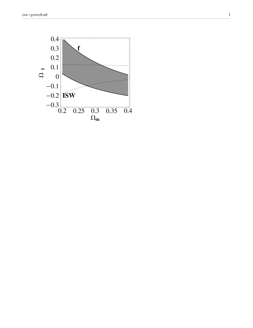
Figure 1: In this plot we show the constraints on $\Omega_{1}$ from the ISW effect (within the dotted lines) and from the growth rate $f$ of structures (grey region), assuming a present value $\Omega_{m}=0.3\pm 0.1$.

5 Conclusion

We have investigated extensions of quintessence models in which part of the dark energy comes from quadratic-order gravity terms (and corresponding scalar kinetic terms). Even though the models contained no direct coupling of the quintessence scalar field to matter, the effective gravitational coupling ($G_{*}$) in the model acquired a time dependence and the stress parameter $\gamma$ deviates from its general-relativistic value. We included all possible ghost-free second-order gravity terms in our model, since it is natural for them to all be present simultaneously. This can seen, for example, by considering a scalar field which arises from the compactification of an $N$-torus.

The time variation of $G_{*}$ and the value of $\gamma$ depend on the contribution of the higher-order gravity terms in the Friedmann equation, i.e. on the density fractions $\Omega_{i}$. This suggests that by taking them to be small, the constraints can be satisfied. If we take the coupling of the higher-order gravity terms ($\alpha$) to be small, this is indeed the case. On the other hand if we suppose that the variation of the scalar field is small (which the $\Omega_{i}$ are all proportional to), then we find that $\gamma-1$ and $\dot{G}_{*}/G_{*}$ can still be large. This is due to the fact that the higher-order gravity terms can still have a significant effect on perturbations to the scalar field, even when they have little effect on the Friedmann equation.

We considered the possibility of observing the coupled GB term through the matter perturbation growth and through the ISW effect. We found that current data limit $|\Omega_{1}|\lesssim 0.15$, assuming both small $\alpha$ and slow rolling. This implies that the present effect of a coupled GB term is quite limited; on the other hand, its impact during other epochs in cosmic history remains unbounded.

The contributions from the higher-order “$k$-essence” scalar kinetic terms ($\Omega_{3,4}$) only affect $\gamma$ and $G_{*}$ indirectly via the dynamics of the scalar field, and so the direct constraints on them are much weaker (and completely absent in our slow-roll limit). However, unless the couplings $\xi_{3,4}$ are unnaturally large, the density fractions $\Omega_{3,4}$ will be smaller than $\Omega_{1}$ by factors of $\dot{\phi}^{2},\dot{\phi}^{3}$ respectively, and thus completely negligible in a slowly rolling expansion. Moreover, we have seen that the slow-roll condition is the less restrictive one, in the sense that any faster dynamics will in general yield (barring chance cancellation) tighter constraints on $\Omega_{i}$ (we have shown this explicitly only in the small-$\alpha$ limit, but we can conjecture it is a general property, since higher-order terms in $\alpha$ will generally also bring in higher-order terms in the time derivatives of $\phi$). Of course it is possible that the corrections to $G_{*}$ coming from the different modifications to gravity will cancel each other, resulting in far weaker constraints. This will generally require fine-tuning, although it could occur naturally as a result of symmetries in the underlying theory.

Finally, we emphasise that the constraints obtained here are restricted to the Einstein frame and to energy conservation. This hypothesis permitted us to disentangle any deviations from general relativity exclusively from the higher-order terms. Relaxing this hypothesis, and also the determination of exact cosmological solutions, are interesting subjects that we leave for future study.

References

References

- [1] N. Arkani-Hamed, S. Dimopoulos and G. R. Dvali, The hierarchy problem and new dimensions at a millimeter, Phys. Lett. B 429, 263 (1998) [hep-ph/9803315] I. Antoniadis, N. Arkani-Hamed, S. Dimopoulos and G. R. Dvali, New dimensions at a millimeter to a Fermi and superstrings at a TeV, Phys. Lett. B 436, 257 (1998) [hep-ph/9804398] L. Randall and R. Sundrum, An alternative to compactification, Phys. Rev. Lett. 83, 4690 (1999) [hep-th/9906064] G. R. Dvali, G. Gabadadze and M. Porrati, 4D gravity on a brane in 5D Minkowski space, Phys. Lett. B 485, 208 (2000) [hep-th/0005016]
- [2] C. Wetterich, Cosmologies with variable Newton’s ’constant’, Nucl. Phys. B 302, 645 (1988) C. Wetterich, Cosmology and the fate of dilatation symmetry, Nucl. Phys. B 302, 668 (1988) C. Wetterich, The Cosmon model for an asymptotically vanishing time dependent cosmological ’constant’, Astron. Astrophys. 301, 321 (1995) [hep-th/9408025]
- [3] T. Damour, G. W. Gibbons and C. Gundlach, Dark matter, time varying G, and a dilaton field, Phys. Rev. Lett. 64, 123 (1990) T. Damour and C. Gundlach, Nucleosynthesis Constraints On An Extended Jordan-Brans-Dicke Theory, Phys. Rev. D 43, 3873 (1991)
- [4] M. Parry, S. Pichler and D. Deeg, Higher-derivative gravity in brane world models, JCAP 0504, 014 (2005) [hep-ph/0502048]
- [5] A. A. Starobinsky, A new type of isotropic cosmological models without singularity, Phys. Lett. B 91, 99 (1980) S. Capozziello, F. Occhionero and L. Amendola, The Phase space view of inflation. 2: Fourth order models, Int. J. Mod. Phys. D 1, 615 (1993)
- [6] S. Capozziello, Curvature quintessence, Int. J. Mod. Phys. D 11, 483 (2002) [gr-qc/0201033] S. M. Carroll, V. Duvvuri, M. Trodden and M. S. Turner, Is cosmic speed-up due to new gravitational physics?, Phys. Rev. D 70, 043528 (2004) [astro-ph/0306438]
- [7] D. Lovelock, The Einstein tensor and its generalizations, J. Math. Phys. 12, 498 (1971)
- [8] B. Zumino, Gravity Theories In More Than Four-Dimensions, Phys. Rept. 137, 109 (1986)
- [9] M Spivak, A comprehensive Introduction to Differential Geometry, Publish or Perish, Houston (1999)
- [10] D. G. Boulware and S. Deser, String Generated Gravity Models, Phys. Rev. Lett. 55, 2656 (1985) C. Charmousis and J. F. Dufaux, General Gauss-Bonnet brane cosmology, Class. Quant. Grav. 19, 4671 (2002) [hep-th/0202107] T. Clunan, S. F. Ross and D. J. Smith, On Gauss-Bonnet black hole entropy, Class. Quant. Grav. 21, 3447 (2004) [gr-qc/0402044] C. Barcelo, R. Maartens, C. F. Sopuerta and F. Viniegra, Stacking a 4D geometry into an Einstein-Gauss-Bonnet bulk, Phys. Rev. D 67, 064023 (2003) [hep-th/0211013] T. Kobayashi and T. Tanaka, Five-dimensional black strings in Einstein-Gauss-Bonnet gravity, Phys. Rev. D 71, 084005 (2005) [gr-qc/0412139]
- [11] C. Charmousis and J. F. Dufaux, Gauss-Bonnet gravity renders negative tension branewolds unstable, Phys. Rev. D 70, 106002 (2004) [hep-th/0311267]
- [12] Y. M. Cho, I. P. Neupane and P. S. Wesson, No ghost state of Gauss-Bonnet interaction in warped background, Nucl. Phys. B 621, 388 (2002) [hep-th/0104227] S. C. Davis, Generalised Israel junction conditions for a Gauss-Bonnet brane world, Phys. Rev. D 67, 024030 (2003) [hep-th/0208205] E. Gravanis and S. Willison, Israel conditions for the Gauss-Bonnet theory and the Friedmann equation on the brane universe, Phys. Lett. B 562, 118 (2003) [hep-th/0209076] P. Bostock, R. Gregory, I. Navarro and J. Santiago, Einstein gravity on the codimension 2 brane?, Phys. Rev. Lett. 92, 221601 (2004) [hep-th/0311074] C. Charmousis and R. Zegers, Matching conditions for a brane of arbitrary codimension, JHEP 0508, 075 (2005) [hep-th/0502170] C. Charmousis and R. Zegers, Einstein gravity on an even codimension brane, Phys. Rev. D 72, 064005 (2005) [hep-th/0502171]
- [13] T. Damour and G. Esposito-Farese, Tensor multiscalar theories of gravitation, Class. Quant. Grav. 9, 2093 (1992)
- [14] B. A. Campbell, M. J. Duncan, N. Kaloper and K. A. Olive, Gravitational dynamics with Lorentz Chern-Simons terms, Nucl. Phys. B 351, 778 (1991)
- [15] D. J. Gross and J. H. Sloan, The quartic effective action for the heterotic string, Nucl. Phys. B 291, 41 (1987) R. R. Metsaev and A. A. Tseytlin, Order alpha-prime (two loop) equivalence of the string equations of motion and the sigma model Weyl invariance conditions: dependence on the dilaton and the antisymmetric tensor, Nucl. Phys. B 293, 385 (1987)
- [16] I. Antoniadis, J. Rizos and K. Tamvakis, Singularity - free cosmological solutions of the superstring effective action, Nucl. Phys. B 415, 497 (1994) [hep-th/9305025] S. Kalara and K. A. Olive, Difficulties for field theoretical inflation in string models, Phys. Lett. B 218, 148 (1989) B. A. Campbell, N. Kaloper and K. A. Olive, An open cosmological model in string theory, Phys. Lett. B 277, 265 (1992) N. E. Mavromatos and J. Rizos, Exact solutions and the cosmological constant problem in dilatonic domain wall higher-curvature string gravity, Int. J. Mod. Phys. A 18, 57 (2003) [hep-th/0205299] N. E. Mavromatos and J. Rizos, String inspired higher-curvature terms and the Randall-Sundrum scenario, Phys. Rev. D 62, 124004 (2000) [hep-th/0008074] P. Binetruy, C. Charmousis, S. C. Davis and J. F. Dufaux, Avoidance of naked singularities in dilatonic brane world scenarios with a Gauss-Bonnet term, Phys. Lett. B 544, 183 (2002) [hep-th/0206089] G. Calcagni, S. Tsujikawa and M. Sami, Dark energy and cosmological solutions in second-order string gravity, Class. Quant. Grav. 22, 3977 (2005) [hep-th/0505193]
- [17] S. Nojiri, S. D. Odintsov and M. Sasaki, Gauss-Bonnet dark energy, Phys. Rev. D 71, 123509 (2005) [hep-th/0504052]
- [18] J. P. Uzan, The fundamental constants and their variation: Observational status and theoretical motivations, Rev. Mod. Phys. 75, 403 (2003) [hep-ph/0205340]
- [19] C. M. Will, The confrontation between general relativity and experiment, gr-qc/0510072
- [20] G. Esposito-Farese, Tests of scalar-tensor gravity, AIP Conf. Proc. 736, 35 (2004) [gr-qc/0409081]
- [21] C. Charmousis, S. C. Davis and J. F. Dufaux, Scalar brane backgrounds in higher order curvature gravity, JHEP 0312, 029 (2003) [hep-th/0309083]
- [22] C. Cartier, J. c. Hwang and E. J. Copeland, Evolution of cosmological perturbations in non-singular string cosmologies, Phys. Rev. D 64, 103504 (2001) [astro-ph/0106197] S. Tsujikawa, R. Brandenberger and F. Finelli, On the construction of nonsingular pre-big-bang and ekpyrotic cosmologies and the resulting density perturbations, Phys. Rev. D 66, 083513 (2002) [hep-th/0207228]
- [23] C. Bambi, M. Giannotti and F. L. Villante, The response of primordial abundances to a general modification of and/or of the early universe expansion rate, Phys. Rev. D 71, 123524 (2005) [astro-ph/0503502]
- [24] J. Peebles, The large-scale structure of the universe, CUP 1980
- [25] D. J. Eisenstein et al. [SDSS Collaboration], Detection of the Baryon Acoustic Peak in the Large-Scale Correlation Function of SDSS Luminous Red Galaxies, Astrophys. J. 633, 560 (2005) [astro-ph/0501171]
- [26] T. Giannantonio et al., A high redshift detection of the integrated Sachs-Wolfe effect, Phys. Rev. D 74, 063520 (2006) [astro-ph/0607572]
- [27] E. Gaztanaga, M. Manera and T. Multamaki, New light on dark cosmos, Mon. Not. Roy. Astron. Soc. 365, 171 (2006) [astro-ph/0407022]
- [28] P. S. Corasaniti, T. Giannantonio and A. Melchiorri, Constraining dark energy with cross-correlated CMB and Large Scale Structure data, Phys. Rev. D 71, 123521 (2005) [astro-ph/0504115]
- [29] T. Koivisto and D. F. Mota, Gauss-Bonnet quintessence: Background evolution, large scale structure and cosmological constraints, hep-th/0609155