1 Introduction

Dirichlet-branes (D-branes) have been essential tools to study non-perturbative aspects of string theories and M-theory since their discovery [1]. Domain walls may give a field theoretical realization of D-branes. For instance, like D-branes, domain walls become Bogomol’nyi-Prasad-Sommerfield (BPS) states preserving the half of supersymmetry (SUSY) in SUSY field theories, and their tensions saturate the Bogomol’nyi bound [2, 3]. They appear as $(1/2,1/2)$ tensorial central charges in the SUSY algebras [4]. BPS domain walls were extensively studied in ${\cal N}=1$ Wess-Zumino models and SUSY gauge theories with four supercharges [5]–[7], and ${\cal N}=2$ SUSY gauge theories (with eight supercharges) and their associated hyper-Kähler nonlinear sigma models [8]–[16]. Coupling these walls to ${\cal N}=1$ SUGRA was discussed in [3, 17] and ${\cal N}=2$ SUGRA was in [18]. Besides walls, vortices in non-Abelian gauge theory have also been extensively studied recently [19]. It has been found that in $d=4$, ${\cal N}=2$ SUSY $U(N_{\rm C})$ gauge theories with matter hypermultiplets (or their associated hyper-Kähler nonlinear sigma models), vortices (or lumps) as strings can end on a wall [20] and can be stretched between parallel walls [21], like configurations made of strings and D-branes. String-wall junction has been studied further in [22, 23]. These models admit more varieties of composite solitons like a monopole (0-brane) attached by vortices (strings) [24, 25] and a string intersection [27]. Lifting up to $d=5$, instanton attached by vortices and intersecting vortices carrying instanton charge were found [25]. These composite solitons in field theory may be regarded as toy models of composite configurations of several D-branes in string theory [28].

Figure 1: Honeycomb web of domain walls. This web divides 37 vacua and has 18 external legs and 19 internal faces. The moduli space corresponds to ${\bf C}P^{36}$ whose dimension is 72.

We can pursue similarities further by moving to junctions of branes. Type IIB string theory is invariant under S-duality which exchanges a fundamental string and a D-string or a NS5-brane and a D5-brane. Several $(p,q)$ strings with NS-NS charge $p$ and R-R charge $q$ can make a junction balancing tensions at a junction point [29]. The $(p,q)$ string webs stretched between multiple parallel D$3$-branes are regarded as 1/4 BPS dyon in the D3-brane effective gauge theory [32, 31]. Several $(p,q)$ 5-branes can also form a junction [33]. Type IIB string theory admits more general configurations made of several connected strings or 5-branes, called string webs or 5-brane webs, respectively. They are 1/4 BPS states and give planer diagrams. On the other hand domain walls in field theory also can form a junction [35]. It was shown [36, 37] that wall junctions preserve a quarter of SUSY and therefore are 1/4 BPS states in $d=4$, ${\cal N}=1$ SUSY field theories. The energy density is bounded from below by two types of central charge densities ${\cal Z}_{\alpha}$ ($\alpha=1,2$) and ${\cal Y}$ with ${\cal Z}_{\alpha}$ for walls perpendicular to the $\alpha$-th direction of two co-dimensions and ${\cal Y}$ for a junction. Subsequently a number of works appeared on domain wall junctions [38]–[43]. An exact solution of a ${\bf Z}_{3}$ symmetric wall junction was constructed in the Wess-Zumino model and its junction charge ${\cal Y}$ was found to be negative [38], which was recognized to be natural later [39]. Exact solutions for ${\bf Z}_{n}$ symmetric wall junctions were also found in nonlinear sigma models [40]. As exact solutions in ${\cal N}=2$ SUSY theories, a domain wall intersection was obtained in hyper-Kähler nonlinear sigma models [42], and a ${\bf Z}_{3}$ symmetric wall junction was presented in $d=4$, ${\cal N}=2$ SUSY $U(1)$ gauge theories with three hypermultiplets in the fundamental representation [43]. Embedding a wall junction to SUGRA was also discussed [44]. In either case, only single junctions have been obtained as exact solutions so far. Domain walls are, however, expected to make a network when many junctions are connected together [45] like webs, although no explicit solutions are available yet. Such domain wall networks are also studied in cosmology [46, 47] typically using numerical simulations instead of explicit solutions. Although a qualitative discussion has been made on partial moduli for a simple junction in the literature [37], no quantitative treatment of a complete moduli space was available so far.

The purpose of this paper is to construct all the solutions of domain wall webs as 1/4 BPS states in $d=4$, ${\cal N}=2$ SUSY $U(N_{\rm C})$ gauge theories with $N_{\rm F}(>N_{\rm C})$ hypermultiplets in the fundamental representation with complex masses. The energy density is saturated by central charge densities ${\cal Z}_{\alpha}$ ($\alpha=1,2$) and ${\cal Y}$ as usual [36, 37]. We find that the moduli space of the $1/4$ BPS equation for wall web in this theory to be the complex Grassmann manifold $G_{N_{\rm F},N_{\rm C}}\simeq SU(N_{\rm F})/[SU(N_{\rm F}-N_{\rm C})\times SU(N_{\rm C})\times U(1)]$. Moreover exact solutions are obtained in the strong gauge coupling limit. Our wall webs contain several external legs and loops whose maximal numbers are determined by $N_{\rm F}$ and $N_{\rm C}$. An amusing illustrative example of the exact solution is displayed in Fig. 1. In the case of the Abelian gauge theory, we work out the correspondence between configurations of wall webs and the moduli space ${\bf C}P^{N_{\rm F}-1}$. In that case we find that the web configurations are naturally expressed by the grid diagrams in the complex $\Sigma$ plane ($\Sigma$ is the complex scalar field in the vector multiplet), which are dual to the web diagrams in the configuration space. While vacua and 1/2 BPS walls correspond to the vertices and segments of the grid diagram, junctions correspond to the faces. We find that the wall charges are proportional to the lengths of edges of the grid diagram whereas the junction charge is to the area of the grid diagram. The grid diagram has been found in the context of $(p,q)$ string/5-brane webs in the superstring theory. Our wall webs have a strong similarity with string/5-brane webs when we identify $(p,q)$ charge with the wall central charges $(Z_{1},Z_{2})$. Therefore these solutions can be called $(p,q)$ wall webs.

The moduli space of 1/4 BPS solutions exhibits an interesting structure. To see it let us first recall our previous result on the moduli space of 1/2 BPS domain walls [11, 12]. In this case, all topological sectors with various dimensions are patched together to form the total moduli space, which is again the complex Grassmann manifold. There zero wall sectors with zero dimension (isolated points) corresponding to vacua are added to make the total moduli space compact. In the case of the moduli space for solutions of 1/4 BPS equations, the moduli space ${\cal M}_{1/4}$ for genuine 1/4 BPS states is obtained by removing the moduli space ${\cal M}_{1/2}$ for 1/2 BPS parallel walls and the moduli space ${\cal M}_{1/1}$ for vacua from the total moduli space ${\cal M}_{\rm tot.}\simeq G_{N_{\rm F},N_{\rm C}}$

$${\cal M}_{\rm tot.}={\cal M}_{1/4}+{\cal M}_{1/2}+{\cal M}_{1/1}.$$ (1.1)

Moreover the moduli space ${\cal M}_{1/4}$ for genuine 1/4 BPS states is further decomposed into topological sectors according to the number of junction points.

This paper is organized as follows. In Sec. 2, 1/4 BPS equations for junctions are obtained and solved. The total moduli space for the wall webs are given and the exact solutions in the strong coupling limit is presented. In Sec. 3 we study the explicit relationship between the moduli parameters and the configuration of the wall webs in the case of Abelian gauge theory with $N_{\rm C}=1$. The junction charge ${\cal Y}$ is shown to be always negative in the Abelian gauge theory. In Sec. 4, we discuss wall junction in more general gauge theories. We present a method to estimate the shape of 1/4 BPS wall junctions once 1/2 BPS parallel wall configurations are known in a corresponding theory with real masses. Sec. 5 is devoted to a discussion. In Appendix A, we show that no additional moduli parameters appear from gauge fields in the case of the $U(1)$ gauge theory.

2 1/4 BPS equations and their solutions

We start with 3+1 dimensional ${\cal N}=2$ supersymmetric $U(N_{\rm C})$ gauge theory with $N_{\rm F}(>N_{\rm C})$ massive hypermultiplets in the fundamental representation. The physical fields contained in this model are a gauge field $W_{\mu}\ (\mu=0,1,2,3)$, real adjoint scalars $\Sigma_{\alpha}\ (\alpha=1,2)$ and gaugino $\lambda^{i}$ in the vector multiplet, and $N_{\rm F}$ complex doublets of scalars $H^{iAr}$ $(r=1,2,\cdots,N_{\rm C},\ A=1,2,\cdots,N_{\rm F},\ i=1,2)$ and its superpartners $\psi^{Ar}$ in the hypermultiplets. We express $N_{\rm C}\times N_{\rm F}$ matrix of the hypermultiplets by $H^{i}$. With the metric $\eta_{\mu\nu}=(+1,-1,-1,-1)$, we obtain the bosonic Lagrangian

$${\cal L} = {\rm Tr}\left[-\frac{1}{2g^{2}}F_{\mu\nu}F^{\mu\nu}+\frac{1}{g^{2}}\sum_{\alpha=1}^{2}\mathcal{D}_{\mu}\Sigma_{\alpha}\mathcal{D}^{\mu}\Sigma_{\alpha}+\mathcal{D}_{\mu}H^{i}\left(\mathcal{D}^{\mu}H^{i}\right)^{\dagger}\right]-V,$$ (2.1)

$$V = {\rm Tr}\left[\frac{1}{g^{2}}\sum_{a=1}^{3}\left(Y^{a}\right)^{2}+\sum_{\alpha=1}^{2}\left(H^{i}M_{\alpha}-\Sigma_{\alpha}H^{i}\right)\left(H^{i}M_{\alpha}-\Sigma_{\alpha}H^{i}\right)^{\dagger}-\frac{1}{g^{2}}\left[\Sigma_{1},\Sigma_{2}\right]^{2}\right],$$ (2.2)

with diagonal mass matrices $M_{1}={\rm diag}\left(m_{1},m_{2},\cdots,m_{N_{\rm F}}\right)$ and $M_{2}={\rm diag}\left(n_{1},n_{2},\cdots,n_{N_{\rm F}}\right)$. Here we define $Y^{a}\equiv\frac{g^{2}}{2}\left(c^{a}{\bf 1}_{N_{\rm C}}-(\sigma^{a})^{j}{{}_{i}}H^{i}(H^{j})^{\dagger}\right)$ with $c^{a}$ the Fayet-Iliopoulos (FI) parameters. In the rest of this paper we choose the FI parameters as $c^{a}=(0,0,c>0)$ by using $SU(2)_{R}$ rotation without loss of generality. The covariant derivatives and the field strength are defined by $\mathcal{D}_{\mu}\Sigma_{\alpha}=\partial_{\mu}\Sigma_{\alpha}+i[W_{\mu},\Sigma_{\alpha}]$, $\mathcal{D}_{\mu}H^{i}=\partial_{\mu}H^{i}+iW_{\mu}H^{i}$ and $F_{\mu\nu}=-i[\mathcal{D}_{\mu},\mathcal{D}_{\nu}]=\partial_{\mu}W_{\nu}-\partial_{\nu}W_{\mu}+i[W_{\mu},W_{\nu}]$, respectively. The supertransformation for spinors is

$$\delta\lambda^{i} = \left(\frac{1}{2}\gamma^{\mu\nu}F_{\mu\nu}+\gamma^{\mu}\mathcal{D}_{\mu}\Sigma_{1}+i\gamma^{5}\gamma^{\mu}\mathcal{D}_{\mu}\Sigma_{2}-\gamma^{5}\left[\Sigma_{1},\Sigma_{2}\right]\right)\varepsilon^{i}+iY^{a}(\sigma^{a})^{i}{{}_{j}}\varepsilon^{j},$$ (2.3)

$$\delta\psi = \sqrt{2}\left[-i\gamma^{\mu}\mathcal{D}_{\mu}H^{i}+\left(\Sigma_{1}H^{i}-H^{i}M_{1}\right)-i\gamma^{5}\left(\Sigma_{2}H^{i}-H^{i}M_{2}\right)\right]\epsilon_{ij}\varepsilon^{j},$$ (2.4)

with $\epsilon_{12}=\epsilon^{12}=1$.

When we turn off all the mass parameters, the vacuum manifold of the above model becomes complex Grassmann manifold $T^{*}G_{N_{\rm F},N_{\rm C}}$ with its size $c$. Once mass parameters $m_{A}+in_{A}$ in $M\equiv M_{1}+iM_{2}$ are turned on and are chosen to be nondegenerate, almost all points of the vacuum manifold are lifted and only ${}_{N_{\rm F}}\!C_{\!N_{\rm C}}=N_{\rm F}!/(N_{\rm C}!(N_{\rm F}-N_{\rm C})!)$ points on the base manifold $G_{N_{\rm F},N_{\rm C}}$ remain as the discrete SUSY vacua [48]. Color and flavor are locked in these vacua. Each vacuum is characterized by a set of $N_{\rm C}$ different flavor indices $\{A_{1},\cdots,A_{N_{\rm C}}\}$ out of $N_{\rm F}$ flavors corresponding to the non-vanishing hypermultiplets as $H^{1rA}=\sqrt{c}\delta^{A_{r}}{{}_{A}},\ H^{2rA}=0$. This vacuum is labeled by $\langle A_{1}A_{2}\cdots A_{N_{\rm C}}\rangle$. Here we suppress phase factors by using global gauge transformations. In these vacua, the complex adjoint scalar $\Sigma\equiv\Sigma_{1}+i\Sigma_{2}$ have the vacuum expectation value determined by the mass parameters of the corresponding flavors

$$\langle\Sigma\rangle_{\langle A_{1}\cdots A_{N_{\rm C}}\rangle}={\rm diag}\left(m_{A_{1}}+in_{A_{1}},m_{A_{2}}+in_{A_{2}},\cdots,m_{A_{N_{\rm C}}}+in_{A_{N_{\rm C}}}\right).$$ (2.5)

Let us next derive 1/4 BPS equations for string webs by usual Bogomol’nyi completion of the energy density. We ignore $H^{2}$ below because it always vanishes for the following 1/4 BPS equations. In the following we simply denote $H^{1}\equiv H$. We consider static configurations which are independent on $x^{3}$ $(\partial_{0}=\partial_{3}=0)$ and set $W_{0}=W_{3}=0$. Then the Bogomol’nyi completion is performed as

$${\cal E} = {\rm Tr}\bigg{[}\frac{1}{g^{2}}\left(F_{12}-i\left[\Sigma_{1},\Sigma_{2}\right]\right)^{2}+\frac{1}{g^{2}}\left(\mathcal{D}_{1}\Sigma_{2}-\mathcal{D}_{2}\Sigma_{1}\right)^{2}+\frac{1}{g^{2}}\left(\mathcal{D}_{1}\Sigma_{1}+\mathcal{D}_{2}\Sigma_{2}-Y^{3}\right)^{2}$$ (2.6)

$$+ \sum_{\alpha=1,2}\left(\mathcal{D}_{\alpha}H-HM_{\alpha}+\Sigma_{\alpha}H\right)\left(\mathcal{D}_{\alpha}H-HM_{\alpha}+\Sigma_{\alpha}H\right)^{\dagger}\bigg{]}+\sum_{\alpha=1,2}\partial_{\alpha}J_{\alpha}+{\cal Y}+{\cal Z}_{1}+{\cal Z}_{2}$$

$$\geq {\cal Y}+{\cal Z}_{1}+{\cal Z}_{2}+\sum_{\alpha=1,2}\partial_{\alpha}J_{\alpha},$$

where the central charge densities are of the form

$${\cal Y}\equiv\frac{2}{g^{2}}\partial_{\alpha}{\rm Tr}\left(\epsilon^{\alpha\beta}\Sigma_{2}\mathcal{D}_{\beta}\Sigma_{1}\right),\quad{\cal Z}_{1}\equiv c\partial_{1}{\rm Tr}\Sigma_{1},\quad{\cal Z}_{2}\equiv c\partial_{2}{\rm Tr}\Sigma_{2}$$ (2.7)

Here we define $J_{\alpha}\equiv{\rm Tr}\Big{[}H(M_{\alpha}H^{\dagger}-H^{\dagger}\Sigma_{\alpha})\Big{]}$ in the last line of Eq. (2.6). Notice that this can’t have any contribution to topological charges after integrating over the $x^{1}$-$x^{2}$ plane. The charge density ${\cal Z}$ counts the domain wall charge $\pi_{0}$ and the charge density ${\cal Y}$ counts the junction charge $\pi_{1}$ in the $x^{1}$-$x^{2}$ plane.

From the condition that the above energy bound is saturated, the BPS equations for domain wall webs can be obtained as

$$F_{12}=i\left[\Sigma_{1},\Sigma_{2}\right],\quad\mathcal{D}_{1}\Sigma_{2}=\mathcal{D}_{2}\Sigma_{1},\quad\mathcal{D}_{1}\Sigma_{1}+\mathcal{D}_{2}\Sigma_{2}=Y^{3},$$ (2.8)

$$\mathcal{D}_{1}H=HM_{1}-\Sigma_{1}H,\quad\mathcal{D}_{2}H=HM_{2}-\Sigma_{2}H.$$ (2.9)

These BPS equations can be also derived from the conservation condition for the part of SUSY defined by the projections $\Gamma_{*}\varepsilon=\varepsilon$ with the following gamma matrices for $\Gamma_{*}$

$$\Gamma_{\rm w}=\gamma^{1}\otimes i\sigma^{3},\quad\Gamma_{\rm w^{\prime}}=-i\gamma^{2}\gamma^{5}\otimes i\sigma^{3},\quad\Gamma_{\rm j}=\gamma^{0}\gamma^{3}\otimes{\bf 1}_{2}.$$ (2.10)

These three gamma matrices commute with each other and the product of any two gives the remaining one. Therefore we conclude that the above BPS Eqs. (2.8) and (2.9) preserve 1/4 SUSY. Note that because of a property ${\gamma^{12}}\varepsilon^{i}=-i\gamma^{5}\varepsilon^{i}$ on the projected Killing spinor, we can rotate the configuration in $z\equiv x^{1}+ix^{2}$ plane with accompanying chiral rotation

$$\left(z,\Sigma,M\right)\to e^{i\theta}\left(z,\Sigma,M\right),\quad\left(\lambda^{i},\psi\right)\to e^{-i\frac{\theta}{2}\gamma^{5}}e^{-\frac{\theta}{2}\gamma^{12}}\left(\lambda^{i},\psi\right),$$ (2.11)

maintaining the same combination of 1/4 SUSY. Then the formulae for the 1/4 BPS equations and the central charges remain intact.

The BPS Eqs.(2.8) and (2.9) reduce to the 1/2 BPS equations for the non-Abelian parallel walls [11, 12] when we turn off both the $x^{2}$-dependence and the mass $M_{2}$. Their solutions and the total moduli space were found in Ref. [11]. Moreover, the Eqs.(2.8) and (2.9) can be derived by performing the Scherk-Schwarz (SS) dimensional reduction once from the other 1/4 BPS system with monopoles, vortices and walls [21], and also derived by SS dimensional reduction twice from another 1/4 BPS system with vortices and instantons [25]. The method developed in Refs. [11, 12, 21, 25] to solve BPS equations can be extended to these 1/4 BPS equations (2.8) and (2.9). At the first step we solve the first two of Eqs.(2.8) and (2.9). Notice that the first two in Eqs.(2.8) are an integrability condition for simultaneous solutions of two equations in Eqs.(2.9) to exist consistently. Solutions of Eq. (2.9) are obtained in terms of $N_{\rm C}\times N_{\rm C}$ non-singular matrix $S(x^{\alpha})$ as

$$H=S^{-1}H_{0}e^{M_{1}x^{1}+M_{2}x^{2}},\quad W_{1}-i\Sigma_{1}=-iS^{-1}\partial_{1}S,\quad W_{2}-i\Sigma_{2}=-iS^{-1}\partial_{2}S.$$ (2.12)

Here $H_{0}$ is an $N_{\rm C}\times N_{\rm F}$ constant complex matrix of rank $N_{\rm C}$. We call $H_{0}$ the moduli matrix because it contains moduli parameters of solutions as we see below. Defining a gauge invariant matrix

$$\Omega\equiv SS^{\dagger}$$ (2.13)

the last of Eqs.(2.8) can be written as

$${1\over cg^{2}}\left[\partial_{1}\left(\partial_{1}\Omega\Omega^{-1}\right)+\partial_{2}\left(\partial_{2}\Omega\Omega^{-1}\right)\right]={\bf 1}_{N_{\rm C}}-\Omega_{0}\Omega^{-1},$$ (2.14)

with a “source”

$$\Omega_{0}\equiv c^{-1}H_{0}e^{2(M_{1}x^{1}+M_{2}x^{2})}H_{0}^{\dagger}.$$ (2.15)

We call Eq. (2.14) the master equation of our 1/4 BPS system (2.8) and (2.9) since all configurations of the physical fields $H$, $\Sigma_{\alpha}$ and $W_{\alpha}$ are determined (with appropriate gauge choice) from the solution $\Omega$. The master equation (2.14) should be solved with appropriate boundary conditions which we will discuss in the following section. Notice that the solutions have to approach vacua sufficiently far from the walls, then $\Omega$ approaches to $\Omega_{0}$ there. The energy density of the BPS wall webs in the right-hand side of Eq. (2.6) can be rewritten in terms of $\Omega$ as

$${\cal E}_{\rm BPS}=\frac{2}{g^{2}}{\rm Tr}\left[\epsilon^{\alpha\beta}\partial_{\alpha}\left(\partial_{2}\Omega\Omega^{-1}\right)\partial_{\beta}\left(\partial_{1}\Omega\Omega^{-1}\right)\right]+\left(\frac{c}{2}-\frac{1}{2g^{2}}\partial_{\alpha}^{2}\right)\partial_{\alpha}^{2}\log\det\Omega,$$ (2.16)

where we use the relation

$$\Sigma_{\alpha}=\frac{1}{2}S^{-1}\partial_{\alpha}\Omega S^{\dagger-1}.$$ (2.17)

One of the advantages of solving the BPS equation partially using the matrix $H_{0}$ in Eq. (2.12) is to identify the moduli of the domain wall webs. The matrix $H_{0}$ contains parameters of solutions, namely moduli parameters. However, $(H_{0},S)$ and $(H_{0}^{\prime},S^{\prime})$ related by the world-volume symmetry

$$H_{0}\to H_{0}^{\prime}=VH_{0},\quad S\to S^{\prime}=VS,$$ (2.18)

with $V\in GL(N_{\rm C},{\bf C})$ give the same configurations for the physical fields. Therefore the independent moduli parameters are given by the equivalence class defined by $(H_{0},S)\sim(H_{0}^{\prime},S^{\prime})$. Then the total moduli space which is just a topological space that consists of all the parameters in the moduli matrix $H_{0}$ is the complex Grassmann manifold

$${\cal M}^{\rm webs}_{\rm tot}\simeq G_{N_{\rm F},N_{\rm C}}=\{H_{0}\ |\ H_{0}\sim VH_{0},\ V\in GL(N_{\rm C},{\bf C})\}.$$ (2.19)

To show conclusively that the Grassmann manifold contained in the moduli matrix $H_{0}$ is the total moduli space, we need to prove the existence and uniqueness of solutions of the master equation (2.14). This task has been accomplished in the case of 1/2 BPS parallel walls in $U(1)$ gauge theories [16]. In the case of the 1/2 BPS parallel walls in $U(N_{\rm C})$ gauge theories, no direct proof is available. However, we have shown that the number of moduli parameters contained in $H_{0}$ are necessary and sufficient as required by the index theorem [22, 15]. As for the 1/4 BPS wall webs, we prove the uniqueness of the master equation (2.14) for the case of the $U(1)$ gauge theories in Appendix. Our proof implies that the master equation (2.14) in the $U(1)$ gauge theories does not generate additional moduli parameters besides those in the moduli matrix $H_{0}$. As for the wall webs in the $U(N_{\rm C})$ gauge theories, neither direct proof nor the index theorem are not known yet. However, in the strong gauge coupling limit the master equation (2.14) reduces to just an algebraic equation as we will show, so that we can verify that all the moduli parameters are contained in the moduli matrix for $U(N_{\rm C})$ as well as $U(1)$ gauge theories. For those cases where a direct proof or index theorem is not available, our result (2.19) is at present based on a conjecture that the solution of the master equation exists and is unique.

The total moduli space (2.19) of solutions of the 1/4 BPS equations (2.8) and (2.9) is a compact manifold. One might feel a little strange because ordinary moduli spaces of solitons have non-compact directions; at least their translational zero modes give non-compact directions. Our compact total moduli space exhibits an interesting structure as follows. To see it let us first recall the fact that solution of our 1/4 BPS equations (2.8) and (2.9), namely the moduli matrix $H_{0}$, contains 1/2 BPS and vacuum states besides 1/4 BPS states. In other words, the compact total moduli space $G_{N_{\rm F},N_{\rm C}}$ includes different sectors, namely ${\cal M}^{\text{webs}}_{1/4}$ for genuine 1/4 BPS states, the moduli space ${\cal M}^{\text{walls}}_{1/2}$ for 1/2 BPS walls and ${\cal M}^{\text{vacua}}_{1/1}$ for discrete SUSY vacua

$${\cal M}^{\rm webs}_{\rm tot}\simeq G_{N_{\rm F},N_{\rm C}}={\cal M}^{\text{webs}}_{1/4}\ \bigcup\ {\cal M}^{\text{walls}}_{1/2}\ \bigcup\ {\cal M}^{\text{vacua}}_{1/1}.$$ (2.20)

Notice that the 1/2 BPS wall sector ${\cal M}^{\text{walls}}_{1/2}$ consists of subspaces for the 1/2 BPS walls which preserve different sets of 1/2 supercharges. After decomposition, each sector of $G_{N_{\rm F},N_{\rm C}}$ in Eq. (2.20) is in fact non-compact except for the vacuum sector. The union of them, however, form the compact manifold when all of them are appropriately patched together. Thus the moduli space for genuine 1/4 BPS states is obtained by removing the moduli spaces for 1/2 BPS walls and for vacua from the total moduli space $G_{N_{\rm F},N_{\rm C}}$. Moreover the moduli space ${\cal M}^{\text{webs}}_{1/4}$ is further decomposed into topological sectors according to the number of junction points. In the next section we will illustrate this decomposition of the total moduli space into 1/4, 1/2, and 1/1 BPS subspaces using several examples in the Abelian model.

This kind of the decomposition of the total moduli space $G_{N_{\rm F},N_{\rm C}}$ has been already observed in Refs. [11, 12] for the 1/2 BPS parallel domain walls. Now, we can reproduce the result for 1/2 BPS walls as a special case of the 1/4 BPS webs. Let us first note that our construction of solving 1/4 BPS equations in terms of the moduli matrix $H_{0}$ is insensitive to the changes of mass parameters, even though changing the mass parameters means changing the theory itself. As was mentioned in the paragraph below Eq. (2.11), our 1/4 BPS system of the webs reduces to the 1/2 BPS system of the parallel walls when we turn off both the $x^{2}$ dependence and the mass $M_{2}$. In that case all the component walls in the webs become parallel each other, so that the 1/4 BPS sector ${\cal M}^{\text{webs}}_{1/4}$ and the 1/2 BPS sector ${\cal M}^{\text{walls}}_{1/2}$ in Eq. (2.20) get together and reproduce new 1/2 BPS sector ${\cal M}^{\text{parallel walls}}_{1/2}$ as the moduli space for the 1/2 BPS parallel walls

$${\cal M}^{\text{webs}}_{1/4}\ \bigcup\ {\cal M}^{\text{walls}}_{1/2}\ \to\ {\cal M}^{\text{parallel walls}}_{1/2}.$$ (2.21)

Then the 1/2 BPS parallel walls again form the same total moduli space $G_{N_{\rm F},N_{\rm C}}$ when these are combined with the vacuum sectors as [11]

$${\cal M}^{\rm walls}_{\rm tot}\simeq G_{N_{\rm F},N_{\rm C}}={\cal M}^{\text{parallel walls}}_{1/2}\ \bigcup\ {\cal M}^{\text{vacua}}_{1/1}.$$ (2.22)

Let us consider the strong gauge coupling limit $g^{2}\to\infty$. In this limit the massive gauged linear sigma model (2.1) and (2.2) reduces to the massive nonlinear sigma model with $T^{*}G_{N_{\rm F},N_{\rm C}}$ as its target space [49, 48]. The fields in the vector multiplet reduce to auxiliary fields which can be expressed in terms of the hypermultiplets using their equations of motion:

$$W_{\alpha}=-ic^{-1}H\partial_{\alpha}H^{\dagger},\quad\Sigma_{\alpha}=c^{-1}HM_{\alpha}H^{\dagger}.$$ (2.23)

Since the left hand side of the master equation (2.14) vanishes in the strong coupling limit, the right-hand side gives just an algebraic equation

$$\Omega^{g\to\infty}=\Omega_{0}=c^{-1}H_{0}e^{2(M_{1}x^{1}+M_{2}x^{2})}H_{0}^{\dagger}.$$ (2.24)

$S$ can be calculated from $\Omega$ by fixing a gauge, and the configuration is exactly obtained by Eq. (2.12). In the case of Abelian gauge theory ($N_{\rm C}=1$) we find configurations of scalar fields up to gauge symmetry as

$$H^{A}=\sqrt{c}\,\frac{H_{0}^{A}e^{m_{A}x^{1}+n_{A}x^{2}}}{\sqrt{\sum_{B=1}^{N_{\rm F}}|H_{0}^{B}|^{2}e^{2(m_{B}x^{1}+n_{B}x^{2})}}}.$$ (2.25)

Note that the central charge ${\cal Y}$ vanishes in this limit, so that only ${\cal Z}$ contributes tension of wall webs. We would like to stress that these solutions contain all the exact solutions of 1/2 BPS domain walls and 1/4 BPS domain wall webs in the massive $T^{*}G_{N_{\rm F},N_{\rm C}}$ nonlinear sigma model. They can have any number of external walls and internal loops in the webs. In the next section we will show several exact solutions of webs in Abelian gauge theory to give examples.

3 Abelian domain wall webs

In this section we will investigate several fundamental properties about the 1/4 BPS wall junctions and its webs in SUSY gauge theories. For simplicity, we consider the Abelian gauge theory $(N_{\rm C}=1)$ in the following. In this case, the moduli matrix $H_{0}$ is an $N_{\rm F}$ component complex vector. As was mentioned in the previous section, $H_{0}$ should be identified with $VH_{0}$ where $V$ is a complex number. Therefore these moduli parameters in $H_{0}$ are the homogeneous coordinate of the complex projective space ${\bf C}P^{N_{\rm F}-1}$. Each point in the moduli space ${\bf C}P^{N_{\rm F}-1}$ expresses a configuration of a wall web, parallel walls or vacuum in the real space $x^{1}$-$x^{2}$.

We will examine properties of 1/4 BPS wall webs and give some examples of the webs in the following subsections without restricting us to the strong gauge coupling limit. Although we cannot solve the master equation (2.14) explicitly in the case of finite gauge couplings, we can clarify several fundamental properties, for example tension, position and orientation of component walls, from informations encoded in the moduli matrix $H_{0}$. We will use the infinite gauge coupling limit merely to illustrate the wall webs explicitly.

3.1 Domain wall

Before studying 1/4 BPS domain wall webs, let us begin with a brief review of the 1/2 BPS single wall in the model with relatively real masses for the hypermultiplets. Although this was already studied in detail in Refs. [11, 12], it should be useful to understand the structure of domain wall webs in the following of this paper.

One should note that 1/2 BPS wall configurations and 1/1 SUSY vacua are also solutions of the 1/4 BPS equations for the wall webs. To illustrate the situation, we consider the $N_{\rm F}=2$ model which has two vacua $\langle 1\rangle$ and $\langle 2\rangle$. Let us first consider a model with real masses ($M_{2}=0$) $M={\rm diag}(\tilde{m}_{1},\tilde{m}_{2}),(\tilde{m}_{1}<\tilde{m}_{2})$ and assume that the configuration depends on only $x^{1}$ and $\Sigma_{2}=0$. We can easily see that the wall configuration conserves 1/2 SUSY given by the projection $\Gamma_{\rm w}\varepsilon=\varepsilon$ with $\Gamma_{\rm w}$ in (2.10), and interpolates between a vacuum $\langle 2\rangle$ at $x^{1}\rightarrow\infty$ and a vacuum $\langle 1\rangle$ at $x^{1}\rightarrow-\infty$. Its tension is expressed as

$$T_{\rm wall}=c\int^{\infty}_{-\infty}dx^{1}\ \partial_{1}\Sigma_{1}=c\big{[}\Sigma_{1}\big{]}^{+\infty}_{-\infty}=c(\tilde{m}_{2}-\tilde{m}_{1})>0.$$ (3.1)

By use of the rotation (2.11) and the shift symmetry $\Sigma\rightarrow\Sigma+\Delta M{\bf 1}_{N_{\rm C}},\ (M\to M-\Delta M{\bf 1}_{N_{\rm F}})$, we easily obtain a wall configuration for the case of a generic complex masses $M={\rm diag}(m_{1}+in_{1},m_{2}+in_{2})$ with $(m_{2}-m_{1})^{2}+(n_{2}-n_{1})^{2}=(\tilde{m}_{2}-\tilde{m}_{1})^{2}$. Therefore, this wall configuration is a 1/2 BPS state which preserves 1/2 SUSY given by the projection $e^{-i\frac{\theta}{2}\gamma^{5}}e^{-\frac{\theta}{2}\gamma^{12}}\Gamma_{\rm w}e^{\frac{\theta}{2}\gamma^{12}}e^{i\frac{\theta}{2}\gamma^{5}}$. Note that the angle $\theta$ correlates the phase of the mass difference $\tan\theta=(m_{2}-m_{1})/(n_{2}-n_{1})$. We also find that this wall configuration is mapped into a straight line segment connecting two vacuum points $m_{1}+in_{1}$ and $m_{2}+in_{2}$ in the complex field space of $\Sigma$, and the wall in the real space of $x^{1}$, $x^{2}$ extends along a straight line perpendicular to that line segment in the field space as seen in Fig. 2.

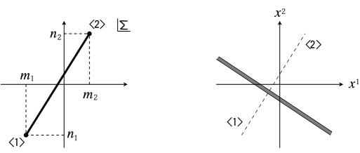
Figure 2: 1/2 BPS domain wall with a complex masses. The left one shows the configuration in the complex $\Sigma$ plane and the right one shows the configuration in the real space.

The tension of the wall per unit length is given by

$$T_{\rm wall}=c\sqrt{(m_{1}-m_{2})^{2}+(n_{1}-n_{2})^{2}}.$$ (3.2)

We can directly derive informations about the wall configuration from the solution given by the moduli matrix

$$H_{0}=\sqrt{c}(e^{a_{1}+ib_{1}},e^{a_{2}+ib_{2}}).$$ (3.3)

Notice that $\log\Omega\sim\log\Omega_{0}$ outside the core of the wall. Then we observe

$$\log\Omega \sim \left\{\begin{array}[]{cl}2(m_{1}x^{1}+n_{1}x^{2}+a_{1})&\text{at\ \ }e^{2(m_{1}x^{1}+n_{1}x^{2}+a_{1})}\gg e^{2(m_{2}x^{1}+n_{2}x^{2}+a_{2})}\\ 2(m_{2}x^{1}+n_{2}x^{2}+a_{2})&\text{at\ \ }e^{2(m_{1}x^{1}+n_{1}x^{2}+a_{1})}\ll e^{2(m_{2}x^{1}+n_{2}x^{2}+a_{2})}\end{array}\right..$$ (3.6)

Let us call

$$(H_{0}e^{M_{1}x^{1}+M_{2}x^{2}})^{A}=e^{a_{A}+m_{A}x^{1}+n_{A}x^{2}}$$ (3.7)

the weight of the vacuum $\langle A\rangle$. The energy density (2.16) becomes negligible far from the core. The wall energy density is concentrated around the transition line separating two vacuum domains, where two terms in $\log\Omega$ are comparable. Namely, the position of the domain wall is determined by the condition of equal weights of the vacua

$$(m_{1}-m_{2})x^{1}+(n_{1}-n_{2})x^{2}+a_{1}-a_{2}=0.$$ (3.8)

Thus we confirm that a wall is orthogonal to the vector $(m_{1}-m_{2},\,n_{1}-n_{2})$.

As was mentioned at the beginning of this section, the total moduli space of the 1/2 BPS single domain wall corresponds to ${\bf C}P^{1}$. It is parametrized by the homogeneous coordinate $H_{0}$ given in Eq. (3.3). From Eqs.(3.3) and (3.8) we realize that a wall configuration is given when we specify a point in ${\bf C}P^{1}$. Namely, generic points in ${\bf C}P^{1}$ give 1/2 BPS configurations of domain walls. However, not all the points of ${\bf C}P^{1}$ give wall configurations. There are two special points in ${\bf C}P^{1}$ manifold which correspond to vacua $\left<1\right>$ and $\left<2\right>$. In terms of the moduli matrix the vacuum $\left<1\right>$ is given by $H_{0}=\sqrt{c}(1,0)$ and the vacuum $\left<2\right>$ by $H_{0}=\sqrt{c}(0,1)$. Both of these can be obtained as limits $a_{2}\to-\infty$ and $a_{1}\to-\infty$ from the generic moduli matrix (3.3), respectively. Physically these can be understood as follows. In the limit $a_{2}\to-\infty$ the weight of the vacuum $\left<2\right>$ vanishes compared to that of the vacuum $\left<1\right>$. Then the domain wall which divides the vacua $\left<1\right>$ and $\left<2\right>$ goes to positive infinity (the position of the wall $a_{1}-a_{2}\rightarrow-\infty$) and the domain $\left<2\right>$ disappears. Similarly, the domain $\left<1\right>$ disappears in the limit $a_{1}\to-\infty$. Thus we conclude that the generic points of ${\bf C}P^{1}\simeq{\bf R}\times S^{1}$ describe domain walls and the remaining two special points are vacua. The total moduli space ${\bf C}P^{1}$ is the union of the subspaces of a one wall sector and zero wall sectors (vacua)

$${\cal M}_{\rm tot}\simeq{\bf C}P^{1}={\cal M}^{\text{1-wall}}_{1/2}\ \bigcup\ {\cal M}^{\text{ vacua}}_{1/1}.$$ (3.9)

3.2 Wall junction

Let us turn our attention to the case of $N_{\rm F}=3$ with 3 discrete vacua labeled by $\left<A\right>$ $(A=1,2,3)$. A 1/4 BPS wall junction firstly appears in this case since a junction is a soliton which divides (at least) three domains (vacua). Similarly to the 1/2 BPS domain wall it is useful to examine the wall junction in the complex $\Sigma$ plane. While the 1/2 BPS wall is mapped to a line segment interpolating two vacua, the 1/4 BPS domain wall junction is mapped onto a triangle whose three vertices are located at points $m_{A}+in_{A}$, as shown in the left figure of Fig. 3. We call polygons in the $\Sigma$ plane as grid diagrams because very similar diagrams which are called grid diagrams appear in papers [34, 33, 31] focusing the $(p,q)$ string/5-brane webs in the superstring theory. Here we assign the complex masses $m_{A}+in_{A}$ so that vacua $\langle 1\rangle,\langle 2\rangle$ and $\langle 3\rangle$ are ordered counterclockwise. As we have seen in the previous subsection, the walls interpolating $\langle A\rangle$ and $\langle B\rangle$ extends in $x^{1}-x^{2}$ plane along the direction perpendicular to the line segment $\langle A\rangle\langle B\rangle$ of the grid diagram, as shown in Fig. 3.

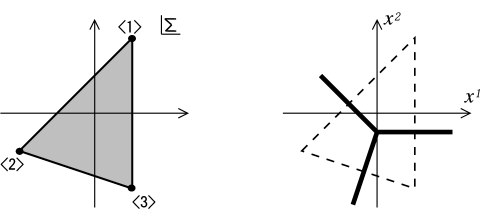
Figure 3: The minimal model for 3-pronged wall junction. The left one is the grid diagram in the complex $\Sigma$ plane and the right one is the web diagram in the configuration space.

Here we give a comment on boundary conditions in solving the master equation (2.14) for 1/4 BPS states of webs. The web has several external legs of walls and then the 1/4 BPS web becomes asymptotically 1/2 BPS single walls at spatial infinities. For the case of the 3-pronged junction, it is useful to take a limit of the triangular boundary whose edges are perpendicular to the external legs of the web. For example, consider a limit of infinite size of the dashed triangle in the right figure of Fig. 3. On each edge of the boundary triangle we should require for the configuration to approach to different 1/2 BPS domain walls. For more complicated webs which have lots of legs and loops as we will deal with in the following, we choose an infinite size limit of polygons whose edges are perpendicular to the external legs as the boundary and require the configuration approaches to the 1/2 BPS walls at the edges.

Each component wall $(A,B)=(1,2),(2,3),(3,1)$ becomes 1/2 BPS in the spacial infinity (along the wall direction) and interpolates vacua from $\left<A\right>$ to $\left<B\right>$. The wall has the tension $\vec{T}^{AB}$ pulling the junction along the wall direction outward

$$\vec{T}^{AB}=(Z_{2}^{AB},-Z_{1}^{AB}),$$ (3.10)

where the central charge of the wall is defined as an integral of ${\cal Z}_{\alpha}$ in Eq. (2.7) over $-\infty<x^{\alpha}<\infty$

$$(Z_{1}^{AB},Z_{2}^{AB})\equiv c(m_{B}-m_{A},n_{B}-n_{A}).$$ (3.11)

The magnitude of the tension is determined by the mass differences similarly to the 1/2 BPS wall as was shown in the previous subsection. We find that these tensions balance at the junction to form a static configuration, $\sum_{AB}\vec{T}^{AB}=0$, because of the conservation of the central charges

$$\sum_{AB}Z_{1}^{AB}=\sum_{AB}Z_{2}^{AB}=0,$$ (3.12)

where $AB$ runs over the labels of legs which extend from the vertex. Therefore the junction configuration can be represented by the web diagram (right figure of Fig. 3) which is obtained by exchanging vertices, edges, and faces of the grid diagram with faces, edges, and vertices, respectively.

We can also read the junction charges geometrically from the grid diagram. Since walls become 1/2 BPS states in the spatial infinity (boundaries), the spatial infinity in the $x^{1}$-$x^{2}$ space are mapped to edges of the grid diagram. Therefore the magnitude of the central charge $Y$ is given by the area of the triangle

$$Y=\int dx^{1}dx^{2}\ {\cal Y}=-\frac{2}{g^{2}}\int_{\triangle}d\Sigma_{1}\wedge d\Sigma_{2}=-{1\over g^{2}}(\Delta m_{1}\Delta n_{2}-\Delta m_{2}\Delta n_{1})<0.$$ (3.13)

where we define $\Delta X_{i}\equiv X_{i}-X_{3},(i=1,2)$ for any quantity $X$. Notice that the contribution of $Y$-charge of the junction to the energy is always negative in the case of the Abelian gauge theories. This negative contribution can be interpreted as a binding energy of wall junction.

Let us now examine the moduli of the junction

$$H_{0}=\sqrt{c}\left(e^{a_{1}+ib_{1}},\ e^{a_{2}+ib_{2}},\ e^{a_{2}+ib_{2}}\right).$$ (3.14)

Positions of the junction can be derived by examining the asymptotic behavior of $\log\Omega$ as we have done for the single domain wall in Eq. (3.6). The wall dividing vacua $\left<A\right>$ and $\left<B\right>$ sits on a half line

$$(m_{A}-m_{B})x^{1}+(n_{A}-n_{B})x^{2}+(a_{A}-a_{B})=0,$$ (3.15)

which is consistent with the condition of the balance of forces given in Eq. (3.12). These three walls get together at the junction position

$$(x^{1},x^{2})=\left(\frac{S_{1}}{S_{3}},\frac{S_{2}}{S_{3}}\right)=\left(\frac{\Delta n_{1}\Delta a_{2}-\Delta n_{2}\Delta a_{1}}{\Delta m_{1}\Delta n_{2}-\Delta m_{2}\Delta n_{1}},\frac{\Delta m_{2}\Delta a_{1}-\Delta m_{1}\Delta a_{2}}{\Delta m_{1}\Delta n_{2}-\Delta m_{2}\Delta n_{1}}\right),$$ (3.16)

where the weights (3.7) of three vacua $\langle 1\rangle,\langle 2\rangle,\langle 3\rangle$ become equal each other. The vector $(S_{1},S_{2},S_{3})=\Delta\vec{v}_{1}\times\Delta\vec{v}_{2}$ is orthogonal to the triangle $\{\vec{v}_{1},\vec{v}_{2},\vec{v}_{3}\},(\vec{v}_{A}=(m_{A},n_{A},a_{A}))$ in three dimensions. This gives a map from a real projective space ${\bf R}P^{2}$ ($\in{\bf C}P^{2}$) to the $x^{1}$-$x^{2}$ space.

For simplicity, let us consider the case with $[m_{A},n_{A}]=\{[1,0],\ [0,1],\ [0,0]\}$. The junction has 3 external legs of walls: $x^{1}=a_{3}-a_{1}$, $x^{2}=a_{3}-a_{2}$ and $x^{2}=x^{1}+a_{1}-a_{2}$. These 3 walls meet at a point $(x^{1},x^{2})=(a_{3}-a_{1},a_{3}-a_{2})$.

Figure 4: The toric diagram for ${\bf C}P^{2}$ which corresponds to the total moduli space of the single 3-pronged junction. Points in the face correspond to the 1/4 BPS junctions, points in the edges to the 1/2 BPS single walls and vertices to the vacua.

Generic points in the total moduli space ${\bf C}P^{2}$ give 1/4 BPS wall junctions.

In Fig. 4, we show the toric diagram (triangle) of ${\bf C}P^{2}$, which has three edges corresponding to the toric diagrams of three ${\bf C}P^{1}$’s, respectively. The generic points in ${\bf C}P^{2}$ are brought to the boundaries by taking moduli parameters $a_{A}$ to minus infinity. In this limit the point on ${\bf C}P^{2}$ moves away from the vertex $\left<A\right>$ and finally it get to the edge $\left<B\right>\left<C\right>$ ($B\neq C\neq A$). Physically this is understood as the weight of the vacuum $\left<A\right>$ vanishes compared to other vacua. Then the domain $\left<A\right>$ disappears, so that the 1/4 BPS junction becomes the 1/2 BPS domain wall interpolating the vacua $\left<B\right>$ and $\left<C\right>$.

As a concrete example, let us consider the limit $a_{1}\to-\infty$ (we call the limit I). In this limit, the junction point $(a_{3}-a_{1},a_{3}-a_{2})$ goes away to plus infinity of $x^{1}$ axis and the only one wall which interpolates vacua $\left<2\right>$ and $\left<3\right>$ remains at $x^{2}=a_{3}-a_{2}$. The moduli matrix $H_{0}$ given in Eq. (3.14) reduces to $\sqrt{c}\left(0,e^{a_{2}+ib_{2}},e^{a_{3}+ib_{3}}\right)$. This corresponds to the moduli matrix (3.3) for the total moduli space ${\bf C}P^{1}$ of the single 1/2 BPS wall.

Figure 5: Three limits I,II and III of the 1/2 BPS 3-pronged junction. Each limit leads to the different 1/2 BPS walls from the 1/4 BPS junction.

When we take the other limit $a_{2}\to-\infty$ or $a_{3}\to-\infty$ (we call the limits II and III) instead of the limit I, the other 1/2 BPS walls remain, see Fig. 5. One can take further limit, for example the limit II, after taking the limit I, where the weight of vacuum $\left<2\right>$ vanishes. Then the wall goes away to infinity and only the vacuum $\left<3\right>$ remains as we showed in the previous subsection.

Thus we conclude that the total moduli space of the 1/4 BPS equation is decomposed into the space of the genuine 1/4 BPS junction and three subspaces for 1/2 BPS walls which conserve different half of supersymmetries and three points (SUSY vacua) as boundaries

$${\cal M}_{\rm tot}\simeq{\bf C}P^{2}={\cal M}^{\rm junction}_{1/4}\ \bigcup\ {\cal M}^{\rm wall}_{1/2}\ \bigcup\ {\cal M}^{\rm vacuum}_{1/1}.$$ (3.17)

Before closing this subsection, we show an exact solution of the wall junction. For that purpose, we take the gauge coupling squared $g^{2}$ to infinity. The solution is given in Eq. (2.25).

(a) energy density		(b) the configuration in $\Sigma$ plane

Figure 6: Exact solution at $g^{2}\to\infty$. The model with hypermultiplet masses $[m_{A},n_{A}]=[1,0],\ [0,1],\ [0,0]$ and with the FI parameter $c=1$. We choose the moduli matrix $H_{0}=(1,1,1)$. In (b), a set of lines $x^{1}+x^{2}={\rm const.}$ are mapped to a set of curved lines in $\Sigma$ plane.

Fig. 6 (a) shows the energy density of the wall junction in real space and Fig. 6 (b) shows the configuration in $\Sigma$ plane. The entire $x^{1}$-$x^{2}$ plane is mapped one-to-one onto the triangle in the $\Sigma$ plane (grid diagram).

3.3 Webs

Domain wall webs which contain 2 or more wall junctions appear in the $U(1)$ gauge theories with $N_{\rm F}\geq 4$. The web diagram (in configuration space) has $N_{\rm F}$ faces (domains) corresponding to the number of vacua. Depending on the values of complex mass parameters of the model, there are two kinds of webs. One is represented by a tree diagram and the other is by a diagram with loops.

Let us consider the simplest example of wall webs in $N_{\rm F}=4$ model with $[m_{A},n_{A}]=\{[1,0],[1,1],[0,1],[0,0]\}$. The moduli matrix which controls the web is of the form

$$H_{0}=\sqrt{c}\left(e^{a_{1}+ib_{1}},e^{a_{2}+ib_{2}},e^{a_{3}+ib_{3}},e^{a_{4}+ib_{4}}\right).$$ (3.18)

These are homogeneous coordinates of the total moduli space ${\bf C}P^{3}$. The corresponding grid diagram is a quadrangle in the $\Sigma$ plane whose vertices are located at $1,1+i,i$ and $0$. Then the web has four external legs. Generally it includes two 3-pronged wall junctions and an internal leg connecting these two junctions therein, as in Fig. 7(a). The 4 external legs of walls are located at $x^{1}=a_{4}-a_{1}$, $x^{2}=a_{4}-a_{3}$, $x^{1}=a_{3}-a_{2}$ and $x^{2}=a_{1}-a_{2}$.

(a) grid diagram		(b) energy density ($g^{2}\to\infty$)

Figure 7: The simplest example of the wall web which has 4 external legs of walls. The model with hypermultiplet masses $[m_{A},n_{A}]=[1,0],\ [1,1],\ [0,1],\ [0,0]$ and with the FI parameter $c=1$. We choose parameters $(a_{1},a_{2},a_{3},a_{4})=(-3,0,-3,0)$.

This web has two branches which we call s- and t-channel. The s-channel appears when we choose the moduli parameters in the region where $a_{1}+a_{3}>a_{2}+a_{4}$. In this region the web has two junctions, s1 dividing vacua $\{\left<4\right>,\left<1\right>,\left<3\right>\}$, and s2 dividing vacua $\{\left<1\right>,\left<2\right>,\left<3\right>\}$. These are located at $(x^{1},x^{2})=(a_{4}-a_{1},a_{4}-a_{3})$ and $(a_{3}-a_{2},a_{1}-a_{2})$, respectively. The internal wall which connects the junctions s1 and s2 is the wall separating vacua $\left<1\right>$ and $\left<3\right>$, as in the left figure of Fig. 8. The transition from s-channel to t-channel and vise versa occurs at the critical point $a_{1}+a_{3}=a_{2}+a_{4}$. At that point two junctions get together and the web has a 4-pronged junction point with 4 external legs emanating from it. The t-channel arises in the region where $a_{1}+a_{3}<a_{2}+a_{4}$. It has two junctions, t1 dividing vacua $\{\left<4\right>,\left<1\right>,\left<2\right>\}$ located at $(a_{4}-a_{1},a_{1}-a_{2})$ and t2 dividing vacua $\{\left<4\right>,\left<2\right>,\left<3\right>\}$ located at $(a_{3}-a_{2},a_{4}-a_{3})$, respectively. The internal wall which connects two junctions in the t-channel is a domain wall separating vacua $\left<2\right>$ and $\left<4\right>$, as in the right figure of Fig. 8.

Figure 8: The s-channel (left) and t-channel (right) in the grid diagram of $N_{\rm F}=4$ case. The middle diagram shows the transition point of s- and t-channel where two junctions meet.

The total moduli space for this web is ${\bf C}P^{3}$. It is coordinatized by the moduli matrix given in Eq. (3.18). The toric diagram for ${\bf C}P^{3}$ is a tetrahedron. The tetrahedron ($\langle 1\rangle\langle 2\rangle\langle 3\rangle\langle 4\rangle$) has a body, 4 faces ($\langle 1\rangle\langle 2\rangle\langle 3\rangle,\cdots$), 6 edges ($\langle 1\rangle\langle 2\rangle,\cdots$), and 4 vertices ($\langle 1\rangle,\langle 2\rangle,\langle 3\rangle,\langle 4\rangle$), as shown in Fig. 9. The generic points in ${\bf C}P^{3}$, namely points in the body of the tetrahedron correspond to the webs which have two 3-pronged junctions (s-channel or t-channel) in Fig. 8 as discussed above. Let us take the limit of one out of four parameters $a_{1},a_{2},a_{3},a_{4}$ going to $-\infty$, which we denote as I,II,III and IV, respectively. Then the rank of moduli matrix is reduced by one. For example, let us consider the limit I.

Figure 9: The toric diagram for ${\bf C}P^{3}$ which is the total moduli space of the web for $N_{\rm F}=4$ model. Points in the body, 4 faces and 6 edges correspond to the web of 2 junctions, the single junctions and the single walls, respectively. The vertices correspond to the vacua.

In the limit the junction point t1 at $\left(a_{4}-a_{1},a_{1}-a_{2}\right)$ is brought to the positive infinity along the direction $(x^{1},x^{2})\propto(1,-1)$. As a result the configuration has only a single junction t2. In fact, the moduli matrix reduces to $H_{0}=\sqrt{c}\left(0,e^{a_{2}+ib_{2}},e^{a_{3}+ib_{3}},e^{a_{4}+ib_{4}}\right)$ which expresses ${\bf C}P^{2}$ for a 3-pronged junction, as in Eq. (3.14). From the viewpoint of the toric diagram of ${\bf C}P^{3}$ this limit corresponds to the procedure where points in the body of the tetrahedron $\left<1\right>\left<2\right>\left<3\right>\left<4\right>$ is taken to points in the face $\left<2\right>\left<3\right>\left<4\right>$. By taking other limits II, III and IV, we can let points in the body $\left<1\right>\left<2\right>\left<3\right>\left<4\right>$ go to points in other faces of ${\bf C}P^{3}$, as illustrated in Fig. 10.

Figure 10: There are 4 limits I, II, III and IV where the web of 2 junctions reduces to the single 3-pronged junction.

After taking one of the limits I, II, III or IV, one can further take another limit. For example, let us take the limit II after taking the limit I (I$\to$II). As a result the junction t2 at $(a_{3}-a_{2},a_{4}-a_{3})$ goes to plus infinity of $x^{1}$ axis. Then we obtain the 1/2 BPS wall dividing vacua $\left<3\right>$ and $\left<4\right>$, as we have shown in the previous subsection. The moduli matrix also reduces to that for ${\bf C}P^{1}$ as $H_{0}=\sqrt{c}\left(0,0,e^{a_{3}+ib_{3}},e^{a_{4}+ib_{4}}\right)$. Moreover, we can take the limit III or IV after taking the limit I and II. In the limit I$\to$II$\to$III, for instance, only the vacuum state $\left<4\right>$ remains and the corresponding moduli matrix reduces to $H_{0}=\sqrt{c}\left(0,0,0,1\right)$.

Thus we conclude that the total moduli space of the 1/4 BPS wall webs in $N_{\rm F}=4$ model is the union of subspaces of a 2-junction sector, 1-junction sectors, single wall sectors and vacua as

$${\cal M}_{\rm tot}\simeq{\bf C}P^{3}={\cal M}^{\text{2-junctions}}_{1/4}\ \bigcup\ {\cal M}^{\text{1-junction}}_{1/4}\ \bigcup\ {\cal M}^{\rm wall}_{1/2}\ \bigcup\ {\cal M}^{\rm vacuum}_{1/1}.$$ (3.19)

For different choices of complex mass parameters in the $N_{\rm F}=4$ model, we can have another type of the wall web which has a loop. In Fig. 11 we show the wall web for the model with $[m_{A},n_{A}]=\{[1,0],[0,1],[-1,-1],[0,0]\}$. This web is described by the moduli matrix in Eq. (3.18). The web has three external legs of walls.

(a) grid diagram		(b) energy density ($g^{2}\to\infty$)

Figure 11: Another example of the web in the $N_{\rm F}=4$ model. The web has 3 external legs and 1 loop. The model with hypermultiplet masses $[m_{A},n_{A}]=[1,0],\ [0,1],\ [-1,-1],\ [0,0]$ and with the FI parameter $c=1$. We choose parameters $(a_{1},a_{2},a_{3},a_{4})=(-1.5,-1.5,-1.5,1.8)$.

Similarly to the s- and t-channel of the tree diagram, this web has also two branches. One branch has a loop with 3 external legs attached and another branch has only a single 3-pronged junction without loops. The loop branch arises in the region $a_{1}+a_{2}+a_{3}<3a_{4}$ and has three 3-pronged junctions which divides three domains $\{\left<4\right>,\left<3\right>,\left<1\right>\}$, $\{\left<4\right>,\left<1\right>,\left<2\right>\}$ and $\{\left<4\right>,\left<2\right>,\left<3\right>\}$, as shown in Fig. 11. Their positions are given by $(a_{4}-a_{1},a_{1}+a_{3}-2a_{4})$, $(a_{4}-a_{1},a_{4}-a_{2})$ and $(a_{2}+a_{3}-2a_{4},a_{4}-a_{2})$, respectively. Similarly to the case of the tree type wall web, we can reduce the loop web to a single 3-pronged junction by taking a limit where one out of three vacua $\left<1\right>$, $\left<2\right>$ and $\left<3\right>$ is taken away to infinity, as in Fig. 12.

Figure 12: The 3 limits I, II, and III, where 2 out of 3 junctions in the loop are brought to infinity.

Namely, take one of $a_{1}$, $a_{2}$ and $a_{3}$ to minus infinity (we denote the limit I, II and III), respectively. From the viewpoint of the toric diagram of ${\bf C}P^{3}$, these limits correspond to letting points in the body of the tetrahedron $\left<1\right>\left<2\right>\left<3\right>\left<4\right>$ to three faces $\left<4\right>\left<2\right>\left<3\right>$, $\left<4\right>\left<3\right>\left<1\right>$ and $\left<4\right>\left<1\right>\left<2\right>$, respectively.

The loop branch can make a transition at the critical point $a_{1}+a_{2}+a_{3}=3a_{4}$ to another branch with a single 3-pronged junction. At that point three 3-pronged junctions in the loop branch get together and the loop shrinks to a junction which divides three domains $\{\left<1\right>,\left<2\right>,\left<3\right>\}$. In the region $a_{1}+a_{2}+a_{3}>3a_{4}$, the vacuum $\langle 4\rangle$ becomes invisible and the parameter $a_{4}$ has almost no effects on the energy density of the web, as illustrated in Fig. 13. The position of the junction is determined by only three parameters $a_{1},a_{2},a_{3}$ as $((a_{2}+a_{3}-2a_{1})/3,(a_{1}+a_{3}-2a_{2})/3)$.

Figure 13: By letting $a_{1}+a_{2}+a_{3}>3a_{4}$, the loop in the web shrinks and reduces to the 3-pronged junction. In the limit IV with $a_{4}\rightarrow-\infty$, the effect of vacuum $\langle 4\rangle$ disappears.

When we take $a_{4}$ to minus infinity (we denote the limit by IV), effect of the vacuum $\left<4\right>$ disappears and the web reduces to the 3-pronged junction completely. Combining this limit IV with the other limits I, II and III, we find four faces of the tetrahedron. Thus we conclude that the total moduli space ${\bf C}P^{3}$ of $N_{\rm F}=4$ loop web is the union of the subspace of several topological sectors as

$${\cal M}_{\rm tot}\simeq{\bf C}P^{3}={\cal M}^{\rm loop}_{1/4}\ \bigcup\ {\cal M}^{\text{1-junction}}_{1/4}\ \bigcup\ {\cal M}^{\rm wall}_{1/2}\ \bigcup\ {\cal M}^{\rm vacuum}_{1/1}.$$ (3.20)

There are special cases where the mass parameters are partially or completely parallel. In such cases a part or whole of the web consists of parallel walls. We show the web with masses $[m_{A},n_{A}]=\{[1,0],[2,0],[0,1],[0,0]\}$ and $[m_{A},n_{A}]=\{[1,0],[2,0],[3,0],[0,0]\}$ in Fig. 14.

Figure 14: Grid diagrams for the special cases where the mass parameters partially or completely parallel. In these case the web has parallel walls therein or consists of parallel walls only.

Next let us consider general cases of $N_{\rm F}$. Suppose we have a grid diagram for the $N_{\rm F}-1$ case. If we add one more flavor with a mass outside of the grid diagram, the number of edges of the grid diagram, that is, the number of external legs in the web diagram increases by one. If we add a flavor with a mass inside of the grid diagram, then three internal legs are added to the web diagram and those form a loop. Therefore the graphical relation for the web diagram is given by

$$N_{\rm F}=F=E_{\rm ext}+L,$$ (3.21)

where $F$ is the number of faces, $E_{\rm ext}$ is the number of external legs and $L$ is the number of loops in the web, respectively. Conversely, this relation implies that there are just enough degrees of freedom to shift external legs and to shrink loops. By removing one of the junctions or reduces one of the loops to a vertex, we obtain configurations corresponding to $N_{\rm F}$ number of ${\bf C}P^{N_{\rm F}-2}$’s as boundaries of ${\bf C}P^{N_{\rm F}-1}$. In Fig. 15 we show examples of webs which contain multiple junctions. The web in Fig. 15 divides 7 vacua and its total moduli space is ${\bf C}P^{6}$. More complicated web is shown in Fig. 1 with 37 vacua and with the total moduli space of ${\bf C}P^{36}$.

Figure 15: Mass parameters are chosen as $[m_{A},n_{A}]=[2,0],\ [1,\sqrt{3}],\ [-1,\sqrt{3}],\ [-2,0]$, $[-1,-\sqrt{3}],\ [1,-\sqrt{3}]$ and $[0,0]$. The left one is the regular hexagon with parameters $(a_{1},a_{2},a_{3},a_{4},a_{5},a_{6},a_{7})=r(1,1,1,1,1,1,0)$ and the right one has $(r/3,-16,r/3,r,r,r,0)$ with $r=-10\sqrt{3}$.

4 Wall Webs in More General Gauge Theories

So far we have considered the $U(1)$ gauge group with identical charges for all the hypermultiplets as the simplest case. As a result we have obtained a 3-pronged junction as the fundamental wall junction. In this section we discuss wall webs in more general gauge theories and show that multi-pronged fundamental junction can exist. To this end, we introduce a method to understand 1/4 BPS junctions from the viewpoint of the 1/2 BPS parallel walls. For simplicity, we restrict ourselves to the case of the $U(1)$ gauge theory to explain such a method. As was mentioned in Sec. 2, our technique of solving the 1/4 BPS equations (2.8) and (2.9) by the moduli matrix $H_{0}$ is valid for any values of mass parameters $m_{A}+in_{A}$. Regardless of mass assignments, the configurations are controlled by the same moduli matrix

$$H_{0}=\sqrt{c}\left(e^{a_{1}+ib_{1}},e^{a_{2}+ib_{2}},\cdots,e^{a_{N_{\rm F}}+ib_{N_{\rm F}}}\right),$$ (4.1)

and the position of wall which interpolates vacua $\left<A\right>$ and $\left<B\right>$ can be estimated by comparing the weight of the vacua as

$$m_{A}x^{1}+n_{A}x^{2}+a_{A}\simeq m_{B}x^{1}+n_{B}x^{2}+a_{B}.$$ (4.2)

This simple formula to determine the approximate positions of walls is applicable to both the 1/2 BPS parallel walls and the 1/4 BPS wall webs. The only difference between them is the slope of the walls in the $x^{1}$-$x^{2}$ plane. Namely, the 1/2 BPS configurations have only parallel walls, while the 1/4 BPS configurations have walls with different slopes which have to meet at some point in $x^{1}$-$x^{2}$ plane to form a junction.

We can understand properties of wall webs approximately by making use of the similarity between the 1/4 BPS states and the 1/2 BPS states as follows. When we slice a configuration of 1/4 BPS wall web along a line $x^{2}=$ constant, for instance, the wall configuration on that line is very close (although not identical in detail) to the corresponding 1/2 BPS wall configuration in the theory with real masses $M_{1}$ [$M_{2}\equiv(n_{1},\cdots,n_{N_{\rm F}})=0$], provided moduli are taken to be $x^{2}$ dependent ($a_{A}+n_{A}x^{2}$ and $a_{B}+n_{B}x^{2}$). This is because positions of walls in a 1/4 BPS wall web can be estimated only from the weights of vacua as in Eq. (4.2), which can be interpreted as 1/2 BPS walls [11, 12] with $x^{2}$ dependent moduli $a_{A}+n_{A}x^{2}$ and $a_{B}+n_{B}x^{2}$. Recall that we can obtain the imaginary part of masses $M_{2}=(n_{1},\cdots,n_{N_{\rm F}})$ from the five dimensional theory with real masses $M_{1}$, by the SS reduction along the $U(1)$ symmetry generated by $\sum_{A}n_{A}T_{A}$, with $T_{A}$ the $U(1)$ symmetry for the $A$-th flavor. Position of walls in the 1/4 BPS wall web can be obtained when the modulus, which is a complex partner of $\sum_{A}n_{A}T_{A}$, is promoted to depend linearly on $x^{2}$. We may call this point of view as the slicing technique.

As a concrete example, let us consider the real mass assignment ($n_{A}=0$) of the $N_{\rm F}=3$ model. To avoid inessential complications, we set $M={\rm diag}(0,1,2)$ in the following. In this case configurations have only parallel walls which are perpendicular to $x^{1}$ axis and $\Sigma_{2}=0$ identically. Of course, they are 1/2 BPS states. There are two walls whose positions are estimated as $x^{1}=a_{1}-a_{2}$ and $x^{1}=a_{2}-a_{3}$ for the walls connecting $\left<1\right>$ to $\left<2\right>$, and $\left<2\right>$ to $\left<3\right>$, respectively. In the region where $a_{1}-a_{2}\ll a_{2}-a_{3}$, namely $a_{2}$ is positive and sufficiently large, we observe two walls and the domain of the vacuum $\left<2\right>$ in the middle. The relative distance is given by $L=2a_{2}-(a_{1}+a_{3})$. Notice that $L$ has a physical meaning as the relative distance only for $L>0$. For $L<0$, the energy density becomes almost independent of $L$. In the limit $a_{2}\to-\infty(L\rightarrow-\infty)$ the weight of the vacuum $\left<2\right>$ vanishes, and the domain $\left<2\right>$ disappears completely. The wall configuration $\Sigma_{1}$ is schematically shown for the 1/2 BPS parallel walls in Fig. 16.

Figure 16: The configuration of the adjoint scalar $\Sigma_{1}$ for the 1/2 BPS parallel walls is schematically shown as a function of $x^{1}$. The left is two walls sector and the right is one wall sector $(a_{2}\to-\infty)$.

Figure 17: The 3 pronged junction of walls. The dashed lines indicate slices of $x^{2}={\rm const.}$. The slices of the configuration can be thought of the 1 wall sector above the junction point, while the 2 walls sector below the junction.

Let us next turn on the imaginary part of the mass parameters. Consider the mass assignment $M={\rm diag}(0,1-i,2)$. In this case we get the 1/4 BPS junction which consists of three semi-infinite walls. Positions of the walls can be estimated from Eq. (4.2) as $x^{1}-x^{2}+a_{2}-a_{1}=0$ for the wall connecting $\left<1\right>$ to $\left<2\right>$, $x^{1}+x^{2}+a_{3}-a_{2}=0$ for $\left<2\right>$ to $\left<3\right>$ and $2x^{1}+a_{3}-a_{1}=0$ for $\left<3\right>$ to $\left<1\right>$. These get together at a junction point

$$\left({a_{1}-a_{3}\over 2},{2a_{2}-a_{1}-a_{3}\over 2}\right).$$ (4.3)

When we slice the 1/4 BPS junction at various values of $x^{2}={\rm const.}$ as illustrated in Fig. 17, the 1/4 BPS junction can be thought of a collection of many 1/2 BPS parallel walls. In fact, if we regard $x^{2}$ as a constant, the estimated positions (4.2) of walls in the 1/4 BPS web can be interpreted as that for 1/2 BPS walls. On a slice at $x^{2}={\rm const.}<a_{2}-(a_{1}+a_{3})/2$, we find a wall dividing $\left<1\right>$ and $\left<2\right>$ at $x^{1}=a_{1}-a_{2}+x^{2}$ and a wall dividing $\left<2\right>$ and $\left<3\right>$ at $x^{1}=a_{2}-a_{3}-x^{2}$. The relative distance between these two walls is given by

$$L(x^{2})=2a_{2}-(a_{1}+a_{3})-2x^{2}.$$ (4.4)

Notice that the distance $L(x^{2})$ vanishes at the junction point (4.3) and the domain of the vacuum $\left<2\right>$ disappears at slices above the junction point, $L(x^{2})<0$. In this way, a change of the slice position ($x^{2}$ in this case) can be regarded as a change of moduli parameter corresponding to the relative distance between parallel 1/2 BPS walls. Therefore we conclude that the 1/4 BPS wall webs can be constructed by promoting the relative distance moduli of the 1/2 BPS parallel walls to a linear function of $x^{2}$ as in Eq. (4.4).

An example. The slicing technique discussed above can be applied to find the shape of 1/4 BPS wall webs qualitatively when we know the 1/2 BPS walls in a theory with real masses. In Ref. [15] we constructed 1/2 BPS wall solution in the $U(1)\times U(1)$ gauge theory with several hypermultiplets with different $U(1)\times U(1)$ charges. In particular we considered the strong gauge coupling limit where the model reduces to a hyper-Kähler nonlinear sigma model with the target space of the cotangent bundle $T^{*}F_{n}$ over the Hirzebruch surface $F_{n}$. We now apply our method to this model.

For one mass arrangement, we find that there are only two moduli parameters for positions of three parallel 1/2 BPS walls, and hence the position of the middle wall is locked [15]. Namely, the relative distance between three walls is controlled by only one moduli parameter. As the relative distance moduli decreases, three walls approach and eventually merge into a single wall. According to the slicing technique discussed above, we should draw a family of slicing lines (dashes lines in the left figure of Fig. 18) progressing to the merging of 3 walls from the left to a point, and then only single wall emerges. Thus we find that a fundamental junction is not a 3-pronged junction but a 4-pronged junction in this case, as in the left figure of Fig. 18.

Interestingly we have completely different physics for another mass arrangement: there exist just two 1/2 BPS walls but when they pass through each other they transmute to another set of walls with different tensions (with total tension unchanged) [15]. In this case also, we get the identical 4-pronged junction when we promote the relative distance between the two walls to a linear function of the coordinate in $x^{1},x^{2}$ plane which is perpendicular to the slicing lines, as shown in the right figure of Fig. 18. Two different physics of 1/2 BPS domain walls for two different mass arrangements [15] just come from differences of the angles of the slices in the same 1/4 BPS wall web.

Figure 18: Left figure: the slices show the three 1/2 BPS parallel walls turning to a single wall. Right figure: the slices show transmutation of 2 parallel walls.

If a model with real masses contains less moduli parameters than the number of walls, positions of multiple 1/2 BPS walls are locked for one mass arrangement. When we turn on complex masses in such a model, a fundamental wall junction will be a multiple-pronged junction in the web diagram.

5 Discussion

In this section we discuss possible future directions of work.

1. Non-Abelian junction. In this paper we have worked out explicit solutions in the Abelian gauge theory and have found that the junction charge $Y$ is always negative in this case. We will show in the subsequent paper [50] that a positive junction charge $Y$ occurs in the non-Abelian gauge theory. Only planar diagrams have appeared in the $U(1)$ gauge theory as discussed in this paper, while non-planar diagrams will appear in non-Abelian gauge theory.

2. Effective field theory on wall webs. We can obtain the effective field theory on the wall webs using the method of Manton [51]. Let us first recall that the single 1/2 BPS wall has a complex moduli parameter associated with the broken translation and $U(1)$ flavor symmetries. After being promoted to a field on the world-volume of walls, the mode function of this complex moduli is normalizable when integrated over its single co-dimension and gives a physical field in the effective theory on the wall. However, the webs exist as objects with two co-dimensions and their external legs extend as semi-infinite lines. Therefore those zero modes which are originally a normalizable physical modes of the external legs now have semi-infinite support along the external legs. Consequently they become non-normalizable modes in the effective theory of wall webs. In other words, the zero modes which change the boundary condition at infinity along the wall direction are no longer physical fields in the effective theory of wall webs. In order to obtain the genuine effective theory on the world-volume of the web, we should fix such non-normalizable moduli parameters.

Figure 19: Left figure: two translational zero (NG) modes. Middle figure: a zero mode to change the size of a loop. This is normalizable and can appear in the effective field theory. Right figure: a zero mode (QNG) to change the shape of the rectangle in one direction. This is non-normalizable and appears as a “coupling constant” in the effective theory.

Zero modes coming from the moduli parameters deforming sizes of loops are the only possible normalizable modes, as seen in the middle figure of Fig. 19. Combined with $U(1)$ zero modes, we thus have $L$ complex massless modes if the web contains $L=N_{\rm F}-E_{\rm ext}$ loops with $E_{\rm ext}$ external legs, as given in Eq. (3.21). We illustrate two examples of the non-normalizable zero modes in the left and the right figures of Fig. 19. The left one of Fig. 19 describes NG modes for broken translational invariance along the $x^{1}$ and $x^{2}$ coordinates, which are accompanied by the NG modes for broken $U(1)$ flavor symmetries. On the other hand, the right one of Fig. 19 describes the zero mode which changes the shape of the rectangular loop. Because this mode is not related to any symmetry, it is not a NG boson and is called a quasi-Nambu-Goldstone (QNG) mode [52]. It is important to distinguish the QNG modes from the NG modes. Since the NG modes for translations have a flat and decoupled metric, background values of the NG modes do not contribute to the effective theory. On the other hand, the QNG modes have a nontrivial coupling with normalizable modes. Namely, the position of the web (the left figure of Fig. 19) does not enter into the effective theory while the shape of the rectangular loop (relative distance between left and right sets of external legs) appears in the effective theory as “coupling constants”.

Next we discuss the SUSY in the effective field theory. Since the webs are $1/4$ BPS states in $d=4$, ${\cal N}=2$ SUSY theory with eight supercharges, two supercharges are conserved by the $d=2$ effective theory. Since the minimum spinor in two dimensions is the (one-component) Majonara-Weyl spinor, possible SUSY is either ${\cal N}=(2,0)$ or $(1,1)$. Let us recall that the remaining two supercharges projected by $\Gamma_{\rm w}$ and $\Gamma_{\rm w^{\prime}}$ in Eqs. (2.10) satisfy the $\gamma^{0}\gamma^{3}\varepsilon=\varepsilon$ coming from the junction projection $\Gamma_{\rm j}$ in Eq. (2.10). Since $\gamma^{0}\gamma^{3}$ can be regarded as the chiral matrix in the $1+1$ dimensions of the $x^{0}$-$x^{3}$ plane, the remaining two SUSY directions have the same chirality. This is also consistent with the fact that all of our moduli parameters are complex, because the $(2,0)$ SUSY requires scalars in scalar supermultiplets to be complex whereas the $(1,1)$ SUSY to be real. Since we have obtained the exact solutions in the strong gauge coupling limit, we may be able to obtain the effective theory explicitly. Thus we will obtain a $(2,0)$ nonlinear sigma model [53] as the effective field theory. Since this model has a renewed interest recently [54], it should be worth to pursue quantum aspects of the effective theory on the wall webs.

3. Index theorem. Let us comment on index theorems. The master equation (2.14) does not generate any additional moduli parameters other than those in $H_{0}$ at least for the $U(1)$ case, because of the uniqueness of the solution of the master equation shown in Appendix. Since the uniqueness of the solution has not been shown in non-Abelian gauge theories, the index theorem should clarify if there are additional moduli. Index theorems can count only normalizable modes. We can argue in the following that the possible additional moduli from the master equation are normalizable and are localized around the junction points, if they exist. First, 1/4 BPS wall webs always become a collection of parallel 1/2 BPS walls sufficiently far from their junction points. Second, we know already that all moduli are contained in the moduli matrix $H_{0}$ for the 1/2 BPS walls, because of the index theorem for 1/2 BPS walls [22]. We thus find that the possible additional moduli in the master equation (2.14) are normalizable, and therefore the index theorem for 1/4 BPS wall webs should tell whether the moduli matrix contains necessary and sufficient number of moduli parameters. Namely the index theorem hopefully tells that the wall web with $L$ loops has only $L$ complex bosonic zero modes as the only additional moduli. If we have more zero modes, they should come from solving the master equation (2.14). This remains as a future problem.

4. Similarity with $(p,q)$ 5-brane webs. The $(p,q)$ 5-branes in the type IIB string theory also can form webs [33]. We have seen that our wall webs have many properties in common with the $(p,q)$ 5-brane webs. Both the wall web and the 5-brane web are 1/4 BPS states. The mass formula for the wall web in terms of complex mass differences is very similar to the mass formula for 5-brane web in terms of RR-charges and NS-NS charges. Of course the condition for the balance of force applies to both webs. Then we reached the grid diagram in the $\Sigma$-plane, whose terminology has been borrowed from the $(p,q)$ 5-brane webs. The dual diagrams of the grid diagrams are webs of walls or the $(p,q)$ 5-brane webs, respectively. The effective field theory on 5-brane webs is $d=5$, ${\cal N}=1$ SUSY gauge theory. The light fields in that effective theory come from the same zero modes as given in Fig. 19  [33]. We thus expect that there should be some similarities between $d=2$, ${\cal N}=(2,0)$ sigma models and $d=5$, ${\cal N}=1$ SUSY gauge theories. This gives a new addition to relations between sigma models and gauge theories observed previously.

The phenomenon discussed above resembles to a Feynman diagram with a 3-point vertex. This idea to interpret a web diagram as a Feynman diagram has been known for 5-brane webs and is called the topological vertex [55]. We consider that our model offers an explicit and tractable example of the topological vertex in lower dimensions.

5. Similarity with string webs. We see several similarities between wall webs and 1/4 BPS dyon as string webs [32, 31]. Another interesting correspondence may be the one between monopoles in ${\cal N}=4$ gauge theories and walls in ${\cal N}=2$ gauge theories [56]. The 1/4 BPS dyon can exist in theories with gauge group $SU(N_{\rm C})$ with $N_{\rm C}\geq 3$ [32, 31]. On the other hand 1/4 BPS wall webs can exist if the number of flavors is greater than three, $N_{\rm F}\geq 3$. It is known that this kind of flip of gauge/flavor group always occurs in relation between monopoles and walls.

6. Wall lattice. If the number of hypermultiplets is infinite, we can obtain the wall webs made of infinite number of walls which fill the whole space with infinitely many junctions. Our four dimensional theory can be obtained by the Scherk-Schwarz dimensional reduction from the theory with massless hypermultiplets in six dimensions. When we throw away the Kaluza-Klein (KK) modes we obtain hypermultiplets with masses less than the KK mass. Whereas if we include all KK towers we obtain the infinite number of hypermultiplets with the KK masses. Vacua in this theory becomes points in an infinite lattice in the $\Sigma$ plane. Since a wall can interpolate between a vacuum in a fundamental region to a nearest fundamental region, we obtain infinitely many wall junctions. By suitably choosing moduli parameters we get a lattice of the wall webs with the KK masses, which we may call the wall lattice. The $SL(2,{\bf Z})$ invariance for torus compactification will lead a duality on this wall lattice. Although these infinite wall webs are interesting in their own right, they may become important when one considers applications to cosmology.

Appendix A Uniqueness of the solution of the master equation

In this appendix we show the uniqueness of the master equation (2.14) for the case of the Abelian gauge theory extending the work for walls in Ref. [16]. In that case $\Omega$ and $\Omega_{0}$ are positive definite functions. The master equation can be rewritten as

$$\left(\partial_{1}^{2}+\partial_{2}^{2}\right)\psi=1-\Omega_{0}e^{-\psi},$$ (A.1)

where we redefine the coordinate as $(x^{1},x^{2})\to g\sqrt{c}(x^{1},x^{2})$ and define $\psi\equiv\log\Omega$. Assume that there exist two solutions $\psi$ and $\psi^{\prime}$ of Eq. (A.1) for a given $\Omega_{0}$ with the identical boundary conditions at infinity. Then the difference $\delta\psi=\psi-\psi^{\prime}$ satisfies the equation

$$\left(\partial_{1}^{2}+\partial_{2}^{2}\right)\delta\psi=\Omega_{0}e^{-\psi^{\prime}}\left(1-e^{-\delta\psi}\right),$$ (A.2)

together with the boundary condition $\delta\psi\rightarrow 0$ at the spacial infinity. Since $(1-e^{-\delta\psi})\delta\psi\geq 0$, we find that

$$\delta\psi\cdot\left(\partial_{1}^{2}+\partial_{2}^{2}\right)\delta\psi\geq 0.$$ (A.3)

Suppose $\delta\psi>0$ at a point $x^{1},x^{2}$. Then the boundary condition implies that $\delta\psi$ must have a maximum with a positive value. At a neighborhood of the maximum, $\left(\partial_{1}^{2}+\partial_{2}^{2}\right)\delta\psi$ is always negative, whereas $\delta\psi>0$. Thus we obtain $\delta\psi\cdot\left(\partial_{1}^{2}+\partial_{2}^{2}\right)\delta\psi<0$, contradicting (A.3). Therefore solutions of Eq. (A.2) with the boundary condition $\delta\psi=0$ cannot take positive values anywhere. By a similar argument, we find also that the solutions cannot take negative values. Consequently we conclude that $\delta\psi=0$ is the only solution of Eq. (A.2) with the boundary condition $\delta\psi\rightarrow 0$ at spacial infinity.

References

- [1] J. Polchinski, “String theory. Vol. 1: An introduction to the bosonic string,”; “String theory. Vol. 2: Superstring theory and beyond,” Cambridge, UK: Univ. Pr. (1998).
- [2] E. Witten and D. I. Olive, Phys. Lett. B 78, 97 (1978).
- [3] M. Cvetic, F. Quevedo and S. J. Rey, Phys. Rev. Lett. 67, 1836 (1991); M. Cvetic, S. Griffies and S. J. Rey, Nucl. Phys. B 381, 301 (1992) [arXiv:hep-th/9201007].
- [4] G. R. Dvali and M. A. Shifman, Nucl. Phys. B 504, 127 (1997) [arXiv:hep-th/9611213];
- [5] B. Chibisov and M. A. Shifman, Phys. Rev. D 56, 7990 (1997) [Erratum-ibid. D 58, 109901 (1998)] [arXiv:hep-th/9706141].
- [6] G. R. Dvali and M. A. Shifman, Phys. Lett. B 396, 64 (1997) [Erratum-ibid. B 407, 452 (1997)] [arXiv:hep-th/9612128]; A. Kovner, M. A. Shifman and A. Smilga, Phys. Rev. D 56, 7978 (1997) [arXiv:hep-th/9706089]; A. Smilga and A. Veselov, Phys. Rev. Lett. 79, 4529 (1997) [arXiv:hep-th/9706217]; D. Bazeia, H. Boschi-Filho and F. A. Brito, JHEP 9904, 028 (1999) [arXiv:hep-th/9811084]; V. S. Kaplunovsky, J. Sonnenschein and S. Yankielowicz, Nucl. Phys. B 552, 209 (1999) [arXiv:hep-th/9811195]; G. R. Dvali, G. Gabadadze and Z. Kakushadze, Nucl. Phys. B 562, 158 (1999) [arXiv:hep-th/9901032]; M. Naganuma and M. Nitta, Prog. Theor. Phys. 105, 501 (2001) [arXiv:hep-th/0007184]; D. Binosi and T. ter Veldhuis, Phys. Rev. D 63, 085016 (2001) [arXiv:hep-th/0011113]; N. Maru, N. Sakai, Y. Sakamura and R. Sugisaka, Nucl. Phys. B 616, 47 (2001) [arXiv:hep-th/0107204]; Y. Sakamura, Nucl. Phys. B 656, 132 (2003) [arXiv:hep-th/0207159]; JHEP 0304, 008 (2003) [arXiv:hep-th/0302196].
- [7] M. A. Shifman, Phys. Rev. D 57, 1258 (1998) [arXiv:hep-th/9708060]; M. A. Shifman and M. B. Voloshin, Phys. Rev. D 57, 2590 (1998) [arXiv:hep-th/9709137]; B. S. Acharya and C. Vafa, arXiv:hep-th/0103011; A. Ritz, M. Shifman and A. Vainshtein, Phys. Rev. D 66, 065015 (2002) [arXiv:hep-th/0205083]; Phys. Rev. D 70, 095003 (2004) [arXiv:hep-th/0405175]; A. Ritz, JHEP 0310, 021 (2003) [arXiv:hep-th/0308144].
- [8] E. R. C. Abraham and P. K. Townsend, Phys. Lett. B 291, 85 (1992); Phys. Lett. B 295, 225 (1992); J. P. Gauntlett, D. Tong and P. K. Townsend, Phys. Rev. D 64, 025010 (2001) [arXiv:hep-th/0012178]. D. Tong, Phys. Rev. D 66, 025013 (2002) [arXiv:hep-th/0202012]; JHEP 0304, 031 (2003) [arXiv:hep-th/0303151]; K. S. M. Lee, Phys. Rev. D 67, 045009 (2003) [arXiv:hep-th/0211058]; M. Shifman and A. Yung, Phys. Rev. D 70, 025013 (2004) [arXiv:hep-th/0312257].
- [9] M. Arai, M. Naganuma, M. Nitta, and N. Sakai, Nucl. Phys. B 652, 35 (2003) [arXiv:hep-th/0211103]; “BPS Wall in N=2 SUSY Nonlinear Sigma Model with Eguchi-Hanson Manifold” in Garden of Quanta - In honor of Hiroshi Ezawa, Eds. by J. Arafune et al. (World Scientific Publishing Co. Pte. Ltd. Singapore, 2003) pp 299-325, [arXiv:hep-th/0302028]; M. Arai, E. Ivanov and J. Niederle, Nucl. Phys. B 680, 23 (2004) [arXiv:hep-th/0312037].
- [10] Y. Isozumi, K. Ohashi, and N. Sakai, JHEP 0311, 060 (2003) [arXiv:hep-th/0310189]; JHEP 0311, 061 (2003) [arXiv:hep-th/0310130].
- [11] Y. Isozumi, M. Nitta, K. Ohashi and N. Sakai, Phys. Rev. Lett. 93, 161601 (2004) [arXiv:hep-th/0404198].
- [12] Y. Isozumi, M. Nitta, K. Ohashi and N. Sakai, Phys. Rev. D 70, 125014 (2004) [arXiv:hep-th/0405194].
- [13] Y. Isozumi, M. Nitta, K. Ohashi and N. Sakai, Proceedings of 12th International Conference on Supersymmetry and Unification of Fundamental Interactions (SUSY 04), Tsukuba, Japan, 17-23 Jun 2004, edited by K. Hagiwara et al. (KEK, 2004) p.1 - p.16 [arXiv:hep-th/0409110]; to appear in the proceedings of “NathFest” at PASCOS conference, Northeastern University, Boston, Ma, August 2004 [arXiv:hep-th/0410150].
- [14] M. Eto, Y. Isozumi, M. Nitta, K. Ohashi, K. Ohta and N. Sakai, Phys. Rev. D 71, 125006 (2005) [arXiv:hep-th/0412024].
- [15] M. Eto, Y. Isozumi, M. Nitta, K. Ohashi, K. Ohta, N. Sakai and Y. Tachikawa, Phys. Rev. D 71, 105009 (2005) [arXiv:hep-th/0503033].
- [16] N. Sakai and Y. Yang, arXive:hep-th/0505136.
- [17] M. Cvetic and H. H. Soleng, Phys. Rept. 282, 159 (1997) [arXiv:hep-th/9604090]; M. Eto, N. Maru, N. Sakai and T. Sakata, Phys. Lett. B 553, 87 (2003) [arXiv:hep-th/0208127]; M. Eto, N. Maru and N. Sakai, Nucl. Phys. B 673, 98 (2003) [arXiv:hep-th/0307206]; M. Eto and N. Sakai, Phys. Rev. D 68, 125001 (2003) [arXiv:hep-th/0307276];
- [18] M. Arai, S. Fujita, M. Naganuma and N. Sakai, Phys. Lett. B 556, 192 (2003) [arXiv:hep-th/0212175]; to appear in the proceedings of International Seminar on Supersymmetries and Quantum Symmetries SQS 03, Dubna, Russia, 24-29 Jul 2003, [arXiv:hep-th/0311210]; to appear in the proceedings of SUSY 2003: SUSY in the Desert: 11th Annual International Conference on Supersymmetry and the Unification of Fundamental Interactions, Tucson, Arizona, 5-10 Jun 2003. [arXiv:hep-th/0402040]; M. Eto, S. Fujita, M. Naganuma and N. Sakai, Phys. Rev. D 69, 025007 (2004) [arXiv:hep-th/0306198].
- [19] A. Hanany and D. Tong, JHEP 0307, 037 (2003) [arXiv:hep-th/0306150]. R. Auzzi, S. Bolognesi, J. Evslin, K. Konishi and A. Yung, Nucl. Phys. B 673, 187 (2003) [arXiv:hep-th/0307287]; M. Eto, M. Nitta and N. Sakai, Nucl. Phys. B 701, 247 (2004) [arXiv:hep-th/0405161]; V. Markov, A. Marshakov and A. Yung, Nucl. Phys. B 709, 267 (2005) [arXiv:hep-th/0408235]; A. Gorsky, M. Shifman and A. Yung, Phys. Rev. D 71, 045010 (2005) [arXiv:hep-th/0412082]; M. Shifman and A. Yung, arXiv:hep-th/0501211.
- [20] J. P. Gauntlett, R. Portugues, D. Tong and P. K. Townsend, Phys. Rev. D 63, 085002 (2001) [arXiv:hep-th/0008221]; M. Shifman and A. Yung, Phys. Rev. D 67, 125007 (2003) [arXiv:hep-th/0212293].
- [21] Y. Isozumi, M. Nitta, K. Ohashi and N. Sakai, Phys. Rev. D 71, 065018 (2005) [arXiv:hep-th/0405129].
- [22] N. Sakai and D. Tong, JHEP 0503, 019 (2005) [arXiv:hep-th/0501207];
- [23] R. Auzzi, M. Shifman and A. Yung, arXiv:hep-th/0504148.
- [24] D. Tong, Phys. Rev. D 69, 065003 (2004) [arXiv:hep-th/0307302]; R. Auzzi, S. Bolognesi, J. Evslin and K. Konishi, Nucl. Phys. B 686, 119 (2004) [arXiv:hep-th/0312233]; A. Hanany and D. Tong, JHEP 0404, 066 (2004) [arXiv:hep-th/0403158]; M. Shifman and A. Yung, Phys. Rev. D 70, 045004 (2004) [arXiv:hep-th/0403149]; R. Auzzi, S. Bolognesi and J. Evslin, JHEP 0502, 046 (2005) [arXiv:hep-th/0411074].
- [25] M. Eto, Y. Isozumi, M. Nitta, K. Ohashi and N. Sakai, arXiv:hep-th/0412048.
- [26] M. A. C. Kneipp and P. Brockill, Phys. Rev. D 64, 125012 (2001) [arXiv:hep-th/0104171]; M. A. C. Kneipp, Phys. Rev. D 68, 045009 (2003) [arXiv:hep-th/0211049]; Phys. Rev. D 69, 045007 (2004) [arXiv:hep-th/0308086]; arXiv:hep-th/0401234.
- [27] M. Naganuma, M. Nitta and N. Sakai, Grav. Cosmol. 8, 129 (2002) [arXiv:hep-th/0108133]; R. Portugues and P. K. Townsend, JHEP 0204, 039 (2002) [arXiv:hep-th/0203181].
- [28] A. Hanany and E. Witten, Nucl. Phys. B 492, 152 (1997) [arXiv:hep-th/9611230]; E. Witten, Nucl. Phys. B 500, 3 (1997) [arXiv:hep-th/9703166]; A. Giveon and D. Kutasov, Rev. Mod. Phys. 71, 983 (1999) [arXiv:hep-th/9802067].
- [29] O. Aharony, J. Sonnenschein and S. Yankielowicz, Nucl. Phys. B 474, 309 (1996) [arXiv:hep-th/9603009].
- [30] A. Sen, JHEP 9803, 005 (1998) [arXiv:hep-th/9711130]; S. J. Rey and J. T. Yee, Nucl. Phys. B 526, 229 (1998) [arXiv:hep-th/9711202]; M. Krogh and S. M. Lee, Nucl. Phys. B 516, 241 (1998) [arXiv:hep-th/9712050]; Y. Matsuo and K. Okuyama, Phys. Lett. B 426, 294 (1998) [arXiv:hep-th/9712070]; K. Hashimoto, Prog. Theor. Phys. 101, 1353 (1999) [arXiv:hep-th/9808185]; Y. Imamura, Prog. Theor. Phys. 112, 1061 (2004) [arXiv:hep-th/0410138].
- [31] O. Bergman and B. Kol, Nucl. Phys. B 536, 149 (1998) [arXiv:hep-th/9804160];
- [32] O. Bergman, Nucl. Phys. B 525, 104 (1998) [arXiv:hep-th/9712211]; K. Hashimoto, H. Hata and N. Sasakura, Phys. Lett. B 431, 303 (1998) [arXiv:hep-th/9803127]; Nucl. Phys. B 535, 83 (1998) [arXiv:hep-th/9804164]; K. M. Lee and P. Yi, Phys. Rev. D 58, 066005 (1998) [arXiv:hep-th/9804174]; T. Kawano and K. Okuyama, Phys. Lett. B 432, 338 (1998) [arXiv:hep-th/9804139]; D. Bak, K. Hashimoto, B. H. Lee, H. Min and N. Sasakura, Phys. Rev. D 60, 046005 (1999) [arXiv:hep-th/9901107].
- [33] O. Aharony and A. Hanany, Nucl. Phys. B 504, 239 (1997) [arXiv:hep-th/9704170]; O. Aharony, A. Hanany and B. Kol, JHEP 9801, 002 (1998) [arXiv:hep-th/9710116]; B. Kol and J. Rahmfeld, JHEP 9808, 006 (1998) [arXiv:hep-th/9801067].
- [34] S. Katz, P. Mayr and C. Vafa, Adv. Theor. Math. Phys. 1, 53 (1998) [arXiv:hep-th/9706110].
- [35] E. R. C. Abraham and P. K. Townsend, Nucl. Phys. B 351, 313 (1991).
- [36] G. W. Gibbons and P. K. Townsend, Phys. Rev. Lett. 83, 1727 (1999) [arXiv:hep-th/9905196].
- [37] S. M. Carroll, S. Hellerman and M. Trodden, Phys. Rev. D 61, 065001 (2000) [arXiv:hep-th/9905217].
- [38] H. Oda, K. Ito, M. Naganuma and N. Sakai, Phys. Lett. B 471, 140 (1999) [arXiv:hep-th/9910095]; K. Ito, M. Naganuma, H. Oda and N. Sakai, Nucl. Phys. B 586, 231 (2000) [arXiv:hep-th/0004188]; Nucl. Phys. Proc. Suppl. 101, 304 (2001) [arXiv:hep-th/0012182].
- [39] M. A. Shifman and T. ter Veldhuis, Phys. Rev. D 62, 065004 (2000) [arXiv:hep-th/9912162].
- [40] M. Naganuma, M. Nitta and N. Sakai, Phys. Rev. D 65, 045016 (2002) [arXiv:hep-th/0108179]; Proceedings of 3rd International Sakharov Conference On Physics, edited by A. Semikhatov et al. (Scientific World Pub., 2003) p.537 - p.549, [arXiv:hep-th/0210205].
- [41] A. Gorsky and M. A. Shifman, Phys. Rev. D 61, 085001 (2000) [arXiv:hep-th/9909015]; G. Gabadadze and M. A. Shifman, Phys. Rev. D 61, 075014 (2000) [arXiv:hep-th/9910050]; P. K. Townsend, Class. Quant. Grav. 17, 1267 (2000) [arXiv:hep-th/9911154]; D. Binosi and T. ter Veldhuis, Phys. Lett. B 476, 124 (2000) [arXiv:hep-th/9912081]; J. P. Gauntlett, G. W. Gibbons, C. M. Hull and P. K. Townsend, Commun. Math. Phys. 216, 431 (2001) [arXiv:hep-th/0001024]; S. K. Nam and K. Olsen, JHEP 0008, 001 (2000) [arXiv:hep-th/0002176]; J. P. Gauntlett, G. W. Gibbons and P. K. Townsend, Phys. Lett. B 483, 240 (2000) [arXiv:hep-th/0004136]; D. Binosi, M. A. Shifman and T. ter Veldhuis, Phys. Rev. D 63, 025006 (2001) [arXiv:hep-th/0006026]; A. Ritz, M. Shifman and A. Vainshtein, Phys. Rev. D 70, 095003 (2004) [arXiv:hep-th/0405175].
- [42] J. P. Gauntlett, D. Tong and P. K. Townsend, Phys. Rev. D 63, 085001 (2001) [arXiv:hep-th/0007124].
- [43] K. Kakimoto and N. Sakai, Phys. Rev. D 68, 065005 (2003) [arXiv:hep-th/0306077].
- [44] S. M. Carroll, S. Hellerman and M. Trodden, Phys. Rev. D 62, 044049 (2000) [arXiv:hep-th/9911083]; T. Nihei, Phys. Rev. D 62, 124017 (2000) [arXiv:hep-th/0005014].
- [45] P. M. Saffin, Phys. Rev. Lett. 83, 4249 (1999) [arXiv:hep-th/9907066]; D. Bazeia and F. A. Brito, Phys. Rev. Lett. 84, 1094 (2000) [arXiv:hep-th/9908090]; S. K. Nam, JHEP 0003, 005 (2000) [arXiv:hep-th/9911104]; D. Bazeia and F. A. Brito, Phys. Rev. D 61, 105019 (2000) [arXiv:hep-th/9912015]; D. Bazeia and F. A. Brito, Phys. Rev. D 62, 101701 (2000) [arXiv:hep-th/0005045]; F. A. Brito and D. Bazeia, Phys. Rev. D 64, 065022 (2001) [arXiv:hep-th/0105296]; P. Sutcliffe, Phys. Rev. D 68, 085004 (2003) [arXiv:hep-th/0305198].
- [46] H. Kubotani, Prog. Theor. Phys. 87, 387 (1992); R. A. Battye, M. Bucher and D. Spergel, arXiv:astro-ph/9908047; A. Friedland, H. Murayama and M. Perelstein, Phys. Rev. D 67, 043519 (2003) [arXiv:astro-ph/0205520]; P. P. Avelino, J. C. R. Oliveira and C. J. A. Martins, Phys. Lett. B 610, 1 (2005) [arXiv:hep-th/0503226].
- [47] A. Vilenkin and E. P. S. Shellard, “Cosmic Strings and Other Topological Defects,” Cambridge, UK: Univ. Pr. (1994).
- [48] M. Arai, M. Nitta and N. Sakai, Prog. Theor. Phys. 113, 657 (2005) [arXiv:hep-th/0307274]; to appear in the Proceedings of the 3rd International Symposium on Quantum Theory and Symmetries (QTS3), September 10-14, 2003, [arXiv:hep-th/0401084]; to appear in the Proceedings of the International Conference on “Symmetry Methods in Physics (SYM-PHYS10)” held at Yerevan, Armenia, 13-19 Aug. 2003 [arXiv:hep-th/0401102]; to appear in the Proceedings of SUSY 2003 held at the University of Arizona, Tucson, AZ, June 5-10, 2003 [arXiv:hep-th/0402065].
- [49] U. Lindström and M. Roček, Nucl. Phys. B 222 (1983) 285.
- [50] M. Eto, Y. Isozumi, M. Nitta, K. Ohashi and N. Sakai, “Webs of Walls II,” in preparation.
- [51] N. S. Manton, Phys. Lett. B 110, 54 (1982).
- [52] W. Buchmuller, S. T. Love, R. D. Peccei and T. Yanagida, Phys. Lett. B 115, 233 (1982); W. Buchmuller, R. D. Peccei and T. Yanagida, Phys. Lett. B 124, 67 (1983); Nucl. Phys. B 227, 503 (1983); K. Higashijima, M. Nitta, K. Ohta and N. Ohta, Prog. Theor. Phys. 98, 1165 (1997) [arXiv:hep-th/9706219]; M. Nitta, Int. J. Mod. Phys. A 14, 2397 (1999) [arXiv: hep-th/9805038]; K. Higashijima and M. Nitta, Prog. Theor. Phys. 103, 635 (2000) [arXiv:hep-th/9911139]; K. Furuta, T. Inami, H. Nakajima and M. Nitta, Prog. Theor. Phys. 106, 851 (2001) [arXiv:hep-th/0106183].
- [53] C. M. Hull and E. Witten, Phys. Lett. B 160, 398 (1985).
- [54] E. Witten, arXiv:hep-th/0504078.
- [55] M. Aganagic, A. Klemm, M. Marino and C. Vafa, Commun. Math. Phys. 254, 425 (2005) [arXiv:hep-th/0305132].
- [56] N. Dorey, JHEP 9811, 005 (1998) [arXiv:hep-th/9806056]; N. Dorey, T. J. Hollowood and D. Tong, JHEP 9905, 006 (1999) [arXiv:hep-th/9902134].