Catching the phantom: the MSSM on the $\mathbb{Z}_{6}$-orientifold

Abstract

These lecture notes give a short introduction of the derivation of the supersymmetric standard model on the $\mathbb{Z}_{6}$-orientifold as published in hep-th/0404055. Untwisted and twisted cycles are constructed and one specific model is discussed in more detail.

1 Introduction

At the time of the writing of this article, intersecting D6-branes in type IIA string theory are already a long-studied topic of perturbative string theory. It started off by the insight that chiral fermions are possible in these models [2] and now has been proven to be a well-justified complementary approach to the heterotic string, for a broader introduction see for instance [3] and references within.

The goal of all these works is to derive the observed $D=4$ low energy spectrum of particle physics from string theory. This requires compactifications with unitary (or orthogonal) gauge factors with gauge groups of the standard model or a GUT theory. In fact, only the standard model is well established experimentally, but extensions like GUT groups [e.g. a flipped $SU(5)$ or $SO(10)$] seem well motivated such that they also deserve a discussion from string theory. The same is true for $N=1$ spacetime supersymmetry, it is not experimentally found, but very well motivated theoretically and it will be searched for at the LHC. In case it was found, predictions for certain parameters of a supersymmetric extension of the standard model from string theory will be needed. But here one also has to mention the familiar problem of string theory in making definite statements, being the large perturbative vacuum degeneracy. In other words, in many cases there are distinct perturbative string theoretical models which agree on some established features of the standard model, but differ in possible extensions. Nevertheless, one hope is still that some regions of parameter space are at least excluded on the one hand and that maybe on the other hand some model features always appear together like for instance three quark generations with the same rank of the gauge group. It has to be said that so far, we can only make such statements for a very specific perturbative theory, like for instance for a certain $\mathbb{Z}_{n}$-orientifold in type IIA. In recent times, a new approach has been proposed by Douglas [4] which is now commonly called the landscape. In this picture, the idea is not anymore to understand why we live in a specific vacuum of string theory, but instead to use statistics for getting an overall picture of the landscape of all vacua (which has been estimated to be at least $10^{100}$ different flux vacua, see [5] and references within).

The presented paper [1] contributes to this approach in the sense that it gives a complete classification of models on the $\mathbb{Z}_{6}$-orientifold, although statistical tools are actually not needed.

After having specified a certain perturbative string theory (here we will use type II plus additional D-branes), two questions still remain open. One tries to make reasonable assumptions for these two questions and later tries to justify them in a bottom-up approach.

The first one asks for the nature of the six-dimensional compact subspace of the ten spacetime dimensions. Several approaches have been pursued recently: most universal, general Calabi-Yau spaces have been treated in [6]. In this approach, there is the problem that generally only the R-R tadpole and the chiral massless spectrum can be determined by homological data. The NS-NS tadpoles and the non-chiral massless spectrum cannot be determined without a CFT calculation which is only in some cases available. A large subset of such cases are the orientifolded and orbifolded toroidal models, which will be discussed soon. Another alternative case where a CFT description is available are the so-called Gepner or Minimal models which have led to decent phenomenological models within the last year [7, 8].

The second open question asks which objects are living in spacetime, meaning in the present context the D-brane and orientifold content of the theory. Of course, both objects are not independent of the given spacetime. The orientifold planes, being non-dynamical objects, actually are completely defined by dividing out some worldsheet and spacetime groups of the original spacetime, so this already depends on the answer to the first question. On the other hand, the D-branes are dynamical objects and for a complete understanding the backreaction onto spacetime has to be taken into account. However, it is not necessary for the calculation of only the tadpole equation and the massless spectrum. For doing this, D6-brane model building in type IIA seems to be very attractive as D6-branes can wrap special Lagrangian 3-cycles of the compact space. This leads to a very geometrical picture which will shortly be discussed in the following section.

2 D6-brane model building

The starting point for our considerations is type I theory on a six-torus $T^{6}$, whose closed string sector corresponds to type IIB string theory if the world sheet parity $\Omega$ has been gauged. Formally, this gauging can be described by the introduction of orientifold 9-planes. In the language of topology, this object is a cross-cap (reversing the orientation of the worldsheet). In this picture, type I theory can be understood as having a stack of 32 parallel D9-branes whose R-R-charge cancels the one from the orientifold plane. If one now adds a constant magnetic F-flux to the system, the requirement to have exactly 32 D9-planes is getting relaxed. In order to perform CFT calculations, from now on it is assumed that the compact 6-torus is factorized into three 2-tori, i.e. $T^{6}=T^{2}\times T^{2}\times T^{2}$.

A simpler way to understand this can be obtained by performing three T-dualities along the y-axes of the three 2-tori. Then the former F-flux on the D9-branes (which in general is assumed to be different for some stacks of D9-branes) gets transformed into D6-branes wrapping complex 1-cycles on every $T^{2}$, altogether a complex 3-cycle [9]. The angles which every brane spans with the x-axes of every 2-torus are directly related to the former F-flux by

$$\tan\varphi^{I}=F^{I}.$$ (1)

It can be written in terms of so-called wrapping numbers $n_{I}$ and $m_{I}$ which simply denote the number of times that a certain brane wraps the two fundamental cycles with radius $R_{x}^{I}$ and $R_{y}^{I}$ of the $I$th 2-torus, $\tan\varphi^{I}={m_{I}R_{y}^{I}}/{n_{I}R_{x}^{I}}$. The performed T-dualities furthermore map type IIB into IIA theory and the world sheet parity $\Omega$ into the combination $\Omega R$, where $R$ is an anti-holomorphic involution. $R$ is a spacetime symmetry and can often be defined as e.g. a complex conjugation on the complex coordinates of the 2-torus, $R:z_{I}\rightarrow\bar{z}_{I}$. This additional modded out symmetry has the effect that the orientifold plane does also wrap complex 1-cycles on every 2-torus. D6-branes with different angles in general do intersect both among themselves and with the orientifold plane. One obtains a very geometric picture as shown in figure 1.

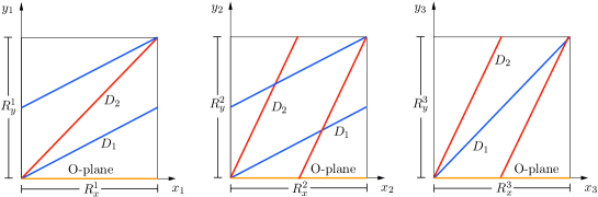
Figure 1: A simple example of intersecting D6-branes on the $\Omega R$-orientifold.

In the present case, one has to add a so-called mirror brane for every D6-brane to the system in order to keep $\Omega R$ invariance. In general, every stack of $N_{i}$ coinciding D6-branes at a particular angle supports a $U(N_{i})$ gauge factor if it does not coincide with the O6-plane (if it does also $SO$ and $Sp$ groups are possible). In [6] it has been described that the chiral massless spectrum of a certain model only depends on the homological data. Actually, the topological intersection number between different types of stacks of D-branes with themselves or the O-plane corresponds to the multiplicity of certain representations, or in other words, the number of particle generations. This correspondence is stated in table 3 and pictured in figure 3.

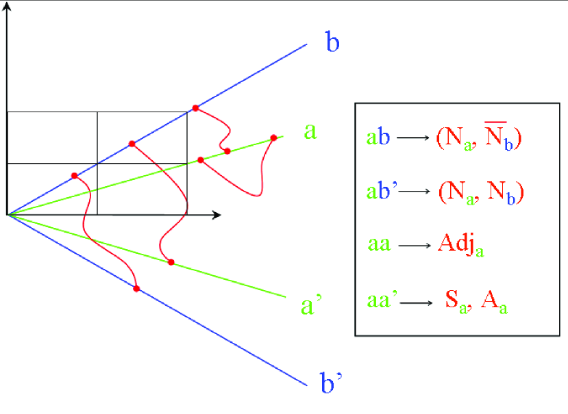
Figure 2: Different topological intersections.

Figure 3: The massless chiral open string spectrum in four dimensions.

representation	multiplicity
$[{\bf A_{a}}]_{L}$	${1\over 2}\left(\pi^{\prime}_{a}\circ\pi_{a}+\pi_{{\rm O}6}\circ\pi_{a}\right)$
$[{\bf S_{a}}]_{L}$	${1\over 2}\left(\pi^{\prime}_{a}\circ\pi_{a}-\pi_{{\rm O}6}\circ\pi_{a}\right)$
$[{\bf(\overline{N}_{a},N_{b})}]_{L}$	$\pi_{a}\circ\pi_{b}$
$[{\bf(N_{a},N_{b})}]_{L}$	$\pi^{\prime}_{a}\circ\pi_{b}$

Another important insight is the fact that it is possible to switch on an additional NS-NS 2-form flux $B^{I}$ in the D9-brane picture. This translates into tilted 2-tori on the side of D6-branes, where now generally odd intersections (including three) are possible [10]. As mentioned earlier, the most important restrictions for model building arise from the R-R and NS-NS tadpole equations, where the R-R tadpole equation can be written homologically as

$$\sum_{a=1}^{k}{N}_{a}\ \left(\pi_{a}+\pi^{\prime}_{a}\right)-4\pi_{\rm O6}=0\ .$$ (2)

In the following, only some particular models shall be mentioned that have been discussed in the immense literature, for more models see the references in [3]. These models generally can be divided into two categories, the ones with $N=0$ and with $N=1$ spacetime supersymmetry.

First the $N=0$ models shall be discussed. The toroidal $\Omega R$-orientifold has been discussed in [9] and afterwards models with exactly the standard model gauge groups have been found [11]. But then it was realized that there are some remaining complex structure moduli in these constructions which will let the tori collapse [12, 13]. This problem has been cured in the ${\mathbb{Z}}_{3}$-orientifold, where the complex structure moduli are frozen because of the Hodge number $h_{2,1}=0$, but still the dilaton instability remains.

In recent times, mainly the $N=1$ models have been discussed, starting with the ${\mathbb{Z}}_{2}\times{\mathbb{Z}}_{2}$-orientifold [15, 14]. In these constructions, the complex structure moduli are unconstrained ($h_{2,1}=3$), but there is no stability problem as the NS-NS-tadpoles are cancelled. General problems of these constructions are the presence of exotic matter (as compared to the MSSM), the need of a hidden brane sector (stacks of D-branes which do not intersect with the MSSM ones, but contribute to the tadpole) and the fact that some MSSM particles might have to be constructed as composite ones. Then there has been the ${\mathbb{Z}}_{4}$-orientifold of [16]. Here, $h_{2,1}=7$ and $h_{1,1}=31$, implying that there are contributions from ${\mathbb{Z}}_{2}$-twisted sectors, generally leading to fractional D-branes, which first have been constructed in [17]. In these models, only mutual intersection numbers $(\pi_{a}\circ\pi_{b},\pi_{a}^{\prime}\circ\pi_{b})=\{(0,0),(\pm 1,0),(0,\pm 1)\}$ are possible, so three particle generations do not arise. Nevertheless, some Pati-Salam-models have been obtained which then could lead to a MSSM-like model after a cascade of non-abelian brane recombinations. But exotic chiral massless matter also here was unavoidable. Similar results have been obtained in the ${\mathbb{Z}}_{4}\times{\mathbb{Z}}_{2}$-orientifold [18]. In the following, the ${\mathbb{Z}}_{6}$-orientifold shall be introduced which leads to more promising phenomenological models.

3 The ${\mathbb{Z}}_{6}$-orientifold

The discussed model is type IIA on $T^{6}/\{{\mathbb{Z}}_{6}+\Omega R{\mathbb{Z}}_{6}\}$, where the ${\mathbb{Z}}_{6}$ orbifold acts as a rotation $\theta$ on the three 2-tori with angles $\pi/3$, $\pi/3$ and $-2\pi/3$, respectively. The model is complicated as it involves ${\mathbb{Z}}_{6}$-, ${\mathbb{Z}}_{3}$- and ${\mathbb{Z}}_{2}$-fixed points on the three 2-tori, as shown in figure 4.

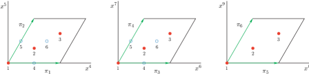
Figure 4: Fixed points of the $T^{6}/{\mathbb{Z}}_{6}$ orbifold, depicted for the AAA torus. Full circles denote $\theta^{2}$ fixed points on $T^{2}_{1}\times T^{2}_{2}$, empty circles additional $\theta^{3}$ fixed points.

The Hodge numbers are given by $h_{2,1}=5$ and $h_{1,1}=29$, implying that there are $b_{3}=2+2h_{2,1}=12$ independent 3-cycles, out of which two arise directly from the torus geometry, being denoted by $\rho$. Furthermore, there are ten additional exceptional 3-cycles $\epsilon$ which are stuck at the ${\mathbb{Z}}_{2}$-fixed points. They have been identified in [1] to be

$$\rho_{1} =2\left(\pi_{1,4,5}+\pi_{1,3,6}+\pi_{2,3,5}-\pi_{1,4,6}-\pi_{2,4,5}-\pi_{2,3,6}\right),$$ (3)

$$\rho_{2} =2\left(\pi_{1,4,5}+\pi_{1,3,6}+\pi_{2,3,5}-\pi_{1,3,5}-\pi_{2,4,6}\right),$$

$$\varepsilon_{1} =\left(e_{41}-e_{61}\right)\otimes\pi_{5}+\left(e_{61}-e_{51}\right)\otimes\pi_{6},$$

$$\tilde{\varepsilon}_{1} =\left(e_{51}-e_{61}\right)\otimes\pi_{5}+\left(e_{41}-e_{51}\right)\otimes\pi_{6},$$

$$\varepsilon_{2} =\left(e_{14}-e_{16}\right)\otimes\pi_{5}+\left(e_{16}-e_{15}\right)\otimes\pi_{6},$$

$$\tilde{\varepsilon}_{2} =\left(e_{15}-e_{16}\right)\otimes\pi_{5}+\left(e_{14}-e_{15}\right)\otimes\pi_{6},$$

$$\varepsilon_{3} =\left(e_{44}-e_{66}\right)\otimes\pi_{5}+\left(e_{66}-e_{55}\right)\otimes\pi_{6},$$

$$\tilde{\varepsilon}_{3} =\left(e_{55}-e_{66}\right)\otimes\pi_{5}+\left(e_{44}-e_{55}\right)\otimes\pi_{6},$$

$$\varepsilon_{4} =\left(e_{45}-e_{64}\right)\otimes\pi_{5}+\left(e_{64}-e_{56}\right)\otimes\pi_{6},$$

$$\tilde{\varepsilon}_{4} =\left(e_{56}-e_{64}\right)\otimes\pi_{5}+\left(e_{45}-e_{56}\right)\otimes\pi_{6},$$

$$\varepsilon_{5} =\left(e_{46}-e_{65}\right)\otimes\pi_{5}+\left(e_{65}-e_{54}\right)\otimes\pi_{6},$$

$$\tilde{\varepsilon}_{5} =\left(e_{54}-e_{65}\right)\otimes\pi_{5}+\left(e_{46}-e_{54}\right)\otimes\pi_{6}.$$

Here, $\pi_{i,j,k}$ just denotes the direct sum of basic exceptional 1-cycles of the three 2-tori, $\pi_{i,j,k}=\pi_{i}\otimes\pi_{j}\otimes\pi_{k}$. The symbols $e_{ij}$ denote the exceptional 2-cycles being stuck at the $i$th ${\mathbb{Z}}_{2}$-fixed point on the first 2-torus and on the $j$th on the second one. The intersection matrices for both types of cycles are given by

$$I_{\rho}=\left(\begin{array}[]{cc}0&-2\\ 2&0\end{array}\right), I_{\varepsilon}=\bigoplus_{j=1}^{5}\left(\begin{array}[]{cc}0&2\\ -2&0\end{array}\right).$$ (8)

These matrices derive from the fact that on the one hand side the exceptional 2-cycles $e_{ij}$ always have a self-intersection number of -2, whereas the intersection numbers of the toroidal cycles have to be taken to be $\pi_{1}\circ\pi_{2}=+1$, but $\pi_{3}\circ\pi_{4}=\pi_{5}\circ\pi_{6}=-1$. This choice of conventions is necessary in order to be able to reproduce the homological computation from the CFT calculation. From this, it is possible to construct a basis of fractional cycles, resembling the topological construction of [17]. The general construction is described in [1], only a typical example shall be given here: a fractional brane can pass through certain ${\mathbb{Z}}_{2}$-fixed points on both the first and second 2-torus, say for instance fixed point 1 on the first and fixed point 4 on the second torus. The corresponding exceptional 2-cycle $e_{14}$ together with its orbifold images $e_{41}$ and $e_{44}$ generate the exceptional 3-cycles $\epsilon_{1}$, $\epsilon_{2}$ and $\epsilon_{3}$. A valid fractional cycle for this case is given by ${1}/{2}\rho_{1}\pm{1}/{2}\left(\varepsilon_{1}\pm\varepsilon_{2}\pm\varepsilon_{3}\right)$.

As for the toroidal orientifold, there are two possibilities for a choice of an automorphism of the ${\mathbb{Z}}_{6}$-invariant lattice. They can be understood as two different orientifold projections of the toroidal 1-cycles, being

$${\bf A}:\left\{\begin{array}[]{l}\pi_{2k-1}\stackrel{{\scriptstyle R}}{{\longrightarrow}}\pi_{2k-1},\\ \pi_{2k}\stackrel{{\scriptstyle R}}{{\longrightarrow}}\pi_{2k-1}-\pi_{2k},\end{array}\right.\qquad\qquad{\bf B}:\pi_{2k-1}\stackrel{{\scriptstyle R}}{{\longleftrightarrow}}\pi_{2k}.$$ (9)

This allows for six inequivalent lattices which are all discussed in [1]. Here only the AAB-torus will be mentioned as it gives the most promising results. The orientifold plane in this case wraps the toroidal cycles $2(\rho_{1}+\rho_{2})$. The action of the orientifold plane onto the toroidal and fractional cycles is given by

$$\rho_{1}\to\rho_{2}, \rho_{2}\to\rho_{1}, \varepsilon_{1}\to-\tilde{\varepsilon}_{1}, \tilde{\varepsilon}_{1}\to-\varepsilon_{1},$$ (10)

$$\varepsilon_{2}\to-\tilde{\varepsilon}_{2}, \tilde{\varepsilon}_{2}\to-\varepsilon_{2}, \varepsilon_{3}\to-\tilde{\varepsilon}_{3}, \tilde{\varepsilon}_{3}\to-\varepsilon_{3},$$

$$\varepsilon_{4}\to-\tilde{\varepsilon}_{5}, \tilde{\varepsilon}_{4}\to-\varepsilon_{5}, \varepsilon_{5}\to-\tilde{\varepsilon}_{4}, \tilde{\varepsilon}_{5}\to-\varepsilon_{4}.$$

Another important condition arises if one demands $N=1$ supersymmetry. For the untwisted cycles one only has to demand the angle criterion. The tree orientated angles which a D-brane geometrically span (w.r.t. the x-axes of the 2-tori) add up to the same angle that the orientifold plane is spanning. This just means that the D-brane has to be calibrated w.r.t. the same holomorphic 3-form as the O-plane in order to be supersymmetric. For the twisted cycles, the conditions turn out to be slightly more involved: in simple terms only those ${\mathbb{Z}}_{2}$-fixed points are allowed to contribute which are traversed by the supersymmetric geometrical part of the brane, for more details see [1].

4 The MSSM on the ${\mathbb{Z}}_{6}$-orientifold

In order to find any phenomenologically interesting supersymmetric models, a computer program has been set up which constructs all possible fractional cycle configurations for a certain number $n$ of D6-brane stacks. For every SUSY untwisted brane, there are altogether 16 possibilities to place the brane on the first 2-tori and switch on Wilson lines and additionally, there are eight different relative ${\mathbb{Z}}_{2}$-eigenvalues. This means that one SUSY untwisted configuration allows for up to $128^{n}$ different supersymmetric fractional brane models. The chiral spectrum for all these configurations which exactly fulfil the R-R and NS-NS tadpole conditions has been systematically calculated up to five stacks. No interesting models with three particle generations and only bifundamental matter has been found for 2,3 or 4 stacks, but the case was very different for five stacks. If one demands that the first three of the five stacks carry a $U(3)$, a $U(2)$ and a $U(1)$ gauge group, respectively, and that there are exactly three left handed quark generations in a $(\bar{\mathbf{3}},\mathbf{2})$ representation and that the sum of right handed $U_{R}$ and $D_{R}$ in $(\mathbf{3},1)$ is six, then there remains exactly one chiral spectrum with just bifundamental matter (although many different concrete realizations on the AAB-torus are possible). This spectrum is shown in table 2, an exemplary concrete realization in homology is given in table 1.

Table 1: The homology cycles and non-vanishing intersection numbers in the 5 stack model on the AAB torus.

homology cycles	intersections
$\Pi_{a}={1\over 2}\left(\rho_{1}+\rho_{2}+\varepsilon_{1}-2\varepsilon_{2}+\varepsilon_{5}-2\tilde{\varepsilon}_{1}+\tilde{\varepsilon}_{2}-2\tilde{\varepsilon}_{5}\right)$	$I_{ab}=0$	$I_{ab^{\prime}}=-3$
$\Pi_{b}={1\over 2}\left(\rho_{1}+\rho_{2}-\varepsilon_{1}-2\varepsilon_{2}-\varepsilon_{5}+2\tilde{\varepsilon}_{1}+\tilde{\varepsilon}_{2}+2\tilde{\varepsilon}_{5}\right)$	$I_{ac}=3$	$I_{ac^{\prime}}=3$
$\Pi_{c}={1\over 2}\left(\rho_{1}+\rho_{2}+3\varepsilon_{2}-\varepsilon_{4}+\varepsilon_{5}-3\tilde{\varepsilon}_{2}-\tilde{\varepsilon}_{4}+\tilde{\varepsilon}_{5}\right)$	$I_{bd}=0$	$I_{bd^{\prime}}=3$
$\Pi_{d}={1\over 2}\left(\rho_{1}+\rho_{2}-\varepsilon_{1}+2\varepsilon_{2}-\varepsilon_{5}+2\tilde{\varepsilon}_{1}-\tilde{\varepsilon}_{2}+2\tilde{\varepsilon}_{5}\right)$	$I_{cd}=3$	$I_{cd^{\prime}}=-3$
$\Pi_{e}={1\over 2}\left(\rho_{1}+\rho_{2}+3\varepsilon_{2}+\varepsilon_{4}-\varepsilon_{5}-3\tilde{\varepsilon}_{2}+\tilde{\varepsilon}_{4}-\tilde{\varepsilon}_{5}\right)$	$I_{be}=3$	$I_{be^{\prime}}=3$

Table 2: Chiral spectrum of the model with gauge group $SU(3)_{a}\times SU(2)_{b}\times U(1)_{a}\times U(1)_{b}\times U(1)_{c}\times U(1)_{d}\times U(1)_{e}$.

chiral spectrum of 5 stack model on the AAB torus
	sector	$SU(3)_{a}\times SU(2)_{b}$	$Q_{a}$	$Q_{b}$	$Q_{c}$	$Q_{d}$	$Q_{e}$	$Q_{B-L}$	$Q_{Y}$
$Q_{L}$	ab’	3 $\times$ ($\overline{{\bf 3}},{\bf 2}$)	-1	-1	0	0	0	${1}/{3}$	${1}/{6}$
$U_{R}$	ac	3$\times$ (${\bf 3},1$)	1	0	-1	0	0	$-{1}/{3}$	$-{2}/{3}$
$D_{R}$	ac’	$3\times$ (${\bf 3},1$)	1	0	1	0	0	$-{1}/{3}$	${1}/{3}$
$L$	bd’	3 $\times$ ($1,{\bf 2}$)	0	1	0	1	0	-1	$-{1}/{2}$
$E_{R}$	cd	3 $\times$ ($1,1$)	0	0	1	-1	0	1	1
$N_{R}$	cd’	3 $\times$ ($1,1$)	0	0	-1	-1	0	1	0
	be	3 $\times$ ($1,{\bf 2}$)	0	1	0	0	-1	0	0
	be’	3 $\times$ ($1,{\bf 2}$)	0	1	0	0	1	0	0

It resembles almost exactly the MSSM, but there are two types of representations which transform under an additional gauge group $Q_{e}$ which still need explanation. The application of the generalized Green-Schwarz mechanism gives the result that three of the initial five $U(1)$s are free of triangle anomalies and massless, being $Q_{B-L}=-{1}/{3}Q_{a}-Q_{d}$, $Q_{c}$ and $Q_{e}$. The first one is a $B-L$ symmetry and $Q_{c}$ is twice the component of the right-handed weak isospin. $Q_{e}$ is an additional $U(1)$ symmetry under which only the two additional fields transform, but none of the standard model particles. The model has a massless hypercharge which is given by the combination $Q_{Y}=-{1}/{6}Q_{a}+{1}/{2}Q_{c}-{1}/{2}Q_{d}$.

The two types of additional particles in the chiral fermion spectrum can be understood as the supersymmetric standard model partners of the Higgs fields with a vanishing hypercharge, $H$ and $\bar{H}$. This explanation requires an abelian brane recombination of the two branes $c$ and $e$, triggering the breaking $U(1)_{c}\times U(1)_{e}\rightarrow U(1)_{C}$ in the effective theory. It is shown in detail in [1] that this mechanism always works and in the effective theory even can be understood as a Higgs effect. All these results are indeed very promising and the phenomenology of the whole class of models with this chiral spectrum should be further explored. One of the most burning questions in this context are Yukawa and gauge couplings [19, 20, 21], where it has to be mentioned that these do depend on the internal geometry and the full massless spectrum, and therefore are difficult to calculate. Furthermore, it is likely that they are different for every concrete realization, maybe a statistical approach could rather handle this difficulty.

Acknowledgements

I would like to thank G. Honecker and R. Blumenhagen for interesting discussions and at the same time G. Honecker and J. Rosseel for proofreading this article. This work is supported in part by the European Community’s Human Potential Programme under contract MRTN-CT-2004-005104 ‘Constituents, fundamental forces and symmetries of the universe’. The work of T.O. is supported in part by the FWO - Vlaanderen, project G.0235.05 and by the Federal Office for Scientific, Technical and Cultural Affairs through the ”Interuniversity Attraction Poles Programme – Belgian Science Policy” P5/27.

References

- [1] G. Honecker and T. Ott, arXiv:hep-th/0404055.
- [2] M. Berkooz, M. R. Douglas and R. G. Leigh, Nucl. Phys. B 480 (1996) 265 [arXiv:hep-th/9606139].
- [3] T. Ott, Fortsch. Phys. 52 (2004) 28 [arXiv:hep-th/0309107].
- [4] M. R. Douglas, JHEP 0305 (2003) 046 [arXiv:hep-th/0303194].
- [5] M. R. Douglas, arXiv:hep-ph/0401004.
- [6] R. Blumenhagen, V. Braun, B. Kors and D. Lust, JHEP 0207 (2002) 026 [arXiv:hep-th/0206038].
- [7] T. P. T. Dijkstra, L. R. Huiszoon and A. N. Schellekens, arXiv:hep-th/0403196.
- [8] T. P. T. Dijkstra, L. R. Huiszoon and A. N. Schellekens, arXiv:hep-th/0411129.
- [9] R. Blumenhagen, L. Goerlich, B. Kors and D. Lust, JHEP 0010 (2000) 006 [arXiv:hep-th/0007024].
- [10] R. Blumenhagen, B. Kors and D. Lust, JHEP 0102 (2001) 030 [arXiv:hep-th/0012156].
- [11] L. E. Ibanez, F. Marchesano and R. Rabadan, JHEP 0111 (2001) 002 [arXiv:hep-th/0105155].
- [12] R. Blumenhagen, B. Kors, D. Lust and T. Ott, Nucl. Phys. B 616 (2001) 3 [arXiv:hep-th/0107138].
- [13] R. Blumenhagen, B. Kors, D. Lust and T. Ott, Fortsch. Phys. 50 (2002) 843 [arXiv:hep-th/0112015].
- [14] M. Cvetic, G. Shiu and A. M. Uranga, Phys. Rev. Lett. 87 (2001) 201801 [arXiv:hep-th/0107143].
- [15] M. Cvetic, G. Shiu and A. M. Uranga, Nucl. Phys. B 615 (2001) 3 [arXiv:hep-th/0107166].
- [16] R. Blumenhagen, L. Gorlich and T. Ott, JHEP 0301 (2003) 021 [arXiv:hep-th/0211059].
- [17] D. E. Diaconescu, M. R. Douglas and J. Gomis, JHEP 9802, 013 (1998) [arXiv:hep-th/9712230].
- [18] G. Honecker, Nucl. Phys. B 666 (2003) 175 [arXiv:hep-th/0303015].
- [19] M. Cvetic and I. Papadimitriou, Phys. Rev. D 68 (2003) 046001 [Erratum-ibid. D 70 (2004) 029903] [arXiv:hep-th/0303083].
- [20] D. Lust, P. Mayr, R. Richter and S. Stieberger, Nucl. Phys. B 696 (2004) 205 [arXiv:hep-th/0404134].
- [21] D. Cremades, L. E. Ibanez and F. Marchesano, JHEP 0405 (2004) 079 [arXiv:hep-th/0404229].