An Oscillon in the $\bm{SU(2)}$ Gauged Higgs Model

Abstract

We study classical dynamics in the spherical ansatz for the $SU(2)$ gauge and Higgs fields of the electroweak Standard Model in the absence of fermions and the photon. With the Higgs boson mass equal to twice the gauge boson mass, we numerically demonstrate the existence of oscillons, extremely long-lived localized configurations that undergo regular oscillations in time. We have only seen oscillons in this reduced theory when the masses are in a two-to-one ratio. If a similar phenomenon were to persist in the full theory, it would suggest a preferred value for the Higgs mass.

I Introduction

In a wide range of nonlinear field theories, the existence of nontrivial static solutions has been well established Coleman ; Rajaraman . However, nonlinear field theories can also support “oscillons,” also called “breathers,” which are localized configurations that oscillate without dissipation. Exact solutions of this kind include sine-Gordon breathers DHN and $Q$-balls ColemanQ . A number of numerical and approximate analyses have established the existence of long-lived breathers in theories with even less structure, such as $\phi^{4}$ theory in one dimension Campbell , $\phi^{4}$ theory in three Bogolubsky ; Gleiser ; iball and higher Gleiserd dimensions, higher dimensional sine-Gordon models Wojtek , and monopole systems Forgacs .

Although oscillons are not necessarily exact solutions, they live for extremely long times — in some cases so long that sophisticated analytic arguments are needed to decide their stability Kruskal ; Hsu because numerical experiments never see their decay. For many physics applications, the distinction between an infinite and a very long lifetime is irrelevant. As long as the object’s lifetime is significantly larger than the natural time scales of the problem, it can have significant effects on the dynamics of the theory.

In this Letter we display an oscillon in the gauged $SU(2)$ Higgs model, which is the Standard Model of the weak interactions neglecting electromagnetism and fermions. We set the Higgs mass to be twice the gauge boson mass. We work in the spherical ansatz and numerically evolve the classical equations of motion. Even after extensive runs, exceeding times of 50,000 in natural units, we have never seen this oscillon decay.

II The Model

We consider an $SU(2)$ gauge theory coupled to a doublet Higgs in $3+1$ dimensions. The Lagrangian is

$${\cal L}=\left[-\frac{1}{2}{\rm Tr}\,F^{\mu\nu}F_{\mu\nu}+\frac{1}{2}{\rm Tr}\,\left(D^{\mu}\Phi\right)^{\dagger}D_{\mu}\Phi-\frac{\lambda}{4}\left({\rm Tr}\,\Phi^{\dagger}\Phi-v^{2}\right)^{2}\right]\,,$$ (1)

where

$$F_{\mu\nu}=\partial_{\mu}A_{\nu}-\partial_{\nu}A_{\mu}-ig[A_{\mu},A_{\nu}]\,,\qquad D_{\mu}\Phi=(\partial_{\mu}-igA_{\mu})\Phi\,,\qquad A_{\mu}=A_{\mu}^{a}\sigma^{a}/2\,,$$ (2)

and we have defined the $2\times 2$ matrix $\Phi$ to represent the Higgs doublet $\varphi$ by

$$\Phi(\bm{x},t)=\left(\matrix{\varphi_{2}^{*}&\varphi_{1}\cr-\varphi_{1}^{*}&\varphi_{2}}\right)\ .$$ (3)

We follow the conventions of Farhi , except we use the metric $ds^{2}=dt^{2}-d\bm{x}^{2}$.

The spherical ansatz spherical is given by expressing the gauge field $A_{\mu}$ and the Higgs field $\Phi$ in terms of six real functions $a_{0}(r,t)$, $a_{1}(r,t)$, $\alpha(r,t)$, $\gamma(r,t)$, $\mu(r,t)$ and $\nu(r,t)$:

$$A_{0}(\bm{x},t) = \frac{1}{2g}a_{0}(r,t){\bm{\sigma}}\cdot\bm{\hat{x}}\,,$$ (4)

$$A_{i}(\bm{x},t) = \frac{1}{2g}\,\left[a_{1}(r,t){\bm{\sigma}}\cdot{\bf\hat{x}}\hat{x}_{i}+\frac{\alpha(r,t)}{r}(\sigma_{i}-{\bm{\sigma}}\cdot{\bf\hat{x}}\hat{x}_{i})+\frac{\gamma(r,t)}{r}\epsilon_{ijk}\hat{x}_{j}\sigma_{k}\right]\,,$$ (5)

$$\Phi(\bm{x},t) = \frac{1}{g}[\mu(r,t)+i\nu(r,t){\bm{\sigma}}\cdot\bm{\hat{x}}]\,,$$ (6)

where $\bm{\hat{x}}$ is the unit three-vector in the radial direction and ${\bm{\sigma}}$ are the Pauli matrices. For the fields of the full theory to be regular at the origin, $a_{0}$, $\alpha$, $a_{1}-\alpha/r$, $\gamma/r$ and $\nu$ must vanish as $r\to 0$. The theory reduced to this ansatz has a residual $U(1)$ gauge invariance consisting of gauge transformations of the form $\exp[i\Omega(r,t){\bm{\sigma}}\cdot\bm{\hat{x}}/2]$ with $\Omega(0,t)=0$.

In the spherical ansatz we obtain the reduced Lagrangian density

$${\cal L}(r,t) = \frac{4\pi}{g^{2}}\left[-\frac{1}{4}r^{2}f^{\mu\nu}f_{\mu\nu}+(D^{\mu}\chi)^{*}D_{\mu}\chi+r^{2}(D^{\mu}\phi)^{*}D_{\mu}\phi-\frac{1}{2r^{2}}\left(|\chi|^{2}-1\right)^{2}\phantom{\left(\frac{1^{2}}{1}\right)^{2}}\right.$$ (8)

$$\left.\qquad-\frac{1}{2}(|\chi|^{2}+1)|\phi|^{2}-{\rm Re}(i\chi^{*}\phi^{2})-\frac{\lambda}{g^{2}}\,r^{2}\,\left(|\phi|^{2}-\frac{g^{2}v^{2}}{2}\right)^{2}\right]\,,$$

where the indices now run over $0$ and $1$ and

$$f_{\mu\nu}=\partial_{\mu}a_{\nu}-\partial_{\nu}a_{\mu}\,,\qquad\chi=\alpha+i\left(\gamma-1\right)\,,\qquad\phi=\mu+i\nu\,,$$ (9)

$$D_{\mu}\chi=(\partial_{\mu}-ia_{\mu})\chi\,,\hbox{\quad and \quad}D_{\mu}\phi=\left(\partial_{\mu}-\frac{i}{2}a_{\mu}\right)\phi\,.$$ (10)

Under the reduced $U(1)$ gauge invariance, the complex scalar fields $\chi$ and $\phi$ have charges of $1$ and $1/2$ respectively, $a_{\mu}$ is the gauge field, $f_{\mu\nu}$ is the field strength, and $D_{\mu}$ is the covariant derivative. The indices are raised and lowered with the $1+1$ dimensional metric $ds^{2}=dt^{2}-dr^{2}$.

The equations of motion for the reduced theory are

$$\partial^{\mu}(r^{2}f_{\mu\nu})=i\left[D_{\nu}\chi^{*}\chi-\chi^{*}D_{\nu}\chi\right]+\frac{i}{2}r^{2}\left[D_{\nu}\phi^{*}\phi-\phi^{*}D_{\nu}\phi\right]\,,$$ (11)

$$\left[D^{2}+\frac{1}{r^{2}}(|\chi|^{2}-1)+\frac{1}{2}|\phi|^{2}\right]\chi=-\frac{i}{2}\phi^{2}\,,$$ (12)

$$\left[D^{\mu}r^{2}D_{\mu}+\frac{1}{2}(|\chi|^{2}+1)+\frac{2\lambda}{g^{2}}\,r^{2}\left(|\phi|^{2}-\frac{g^{2}v^{2}}{2}\right)\right]\phi=i\chi\phi^{*}.$$ (13)

Although it is described by six fields, there are only four independent degrees of freedom in the theory, consisting of the three $W$-bosons, each radially polarized, and the massive Higgs. The remaining degrees of freedom are gauge artifacts. We may fix the gauge by setting $a_{0}(r,t)=0$ everywhere in space and time, and then applying a time-independent gauge transformation to set $a_{1}(r,t=0)=0$. For each of the four fields $\mu$, $\nu$, $\alpha$, and $\gamma$, we must specify the profile at $t=0$ as a function of $r$ and the time derivative of the profile at $t=0$ as a function of $r$. The time derivative of $a_{1}(r,t)$ at $t=0$ is then determined by imposing Gauss’s Law (the first equation in (13) with index $\nu=0$). Configurations obeying Gauss’s Law at the initial time will then obey it for all times. Thus we have fully specified the configuration by providing initial value data for $\chi$ and $\phi$ only, reflecting the four real degrees of freedom of the model.

III Numerical Setup

In order to accurately simulate the extremely long lifetimes of oscillons, we require numerical techniques that are highly stable. We discretize the system at the level of the Lagrangian in Eq. (8). We choose a fixed radial lattice spacing $\Delta r$, placing the scalar fields at the sites of the lattice and the gauge field $a_{1}$ on the links. Thus each of the scalar fields $\xi(r,t)$ is replaced by a set of functions $\xi^{\{n\}}(t)$, defined at each lattice point. We use a first-order lattice gauge-covariant derivative given by the replacement

$$D_{r}\xi(r,t)\rightarrow\frac{\xi^{\{n+1\}}(t)\exp[-iea_{1}^{\{n+\frac{1}{2}\}}(t)\Delta r]-\xi^{\{n\}}(t)}{\Delta r}\,,$$ (14)

where $e$ is the charge of the scalar field and $n=r/\Delta r$ labels the lattice point corresponding to radius $r$. We then vary the spatially discretized Lagrangian to obtain second-order accurate lattice equations of motion. In the limit of continuum time evolution, this system has exact conservation of energy and exact gauge invariance, so we can monitor these quantities to detect numerical errors and determine whether our time steps are short enough. (They do not, however, tell us whether our spatial grid is fine enough, because even for a very coarse grid our system conserves energy and is gauge invariant.) In all our simulations, these invariants hold to an accuracy of roughly one part in $10^{6}$, and we see no numerical instabilities even after extremely long runs.

Since we have $a_{0}(r,t)=0$, the covariant time derivative coincides with the ordinary time derivative. Our time evolution is simply second-order differencing with a fixed time step $\Delta t=\Delta r/2$, in which each subsequent time step is computed from the previous two. This approach is stable for $\Delta t<\Delta r$. We note that to monitor the energy conservation and gauge invariance of the solution, it is necessary to compute first-order time derivatives. These derivatives are computed by subtracting the result at $t_{0}$ from the result at $t_{0}+2\Delta t$, to get a second order accurate result at $t_{0}+\Delta t$.

IV Results

We found the oscillon by picking localized initial value data with zero time derivatives, and letting these configurations evolve. For some initial values, the fields dissipate completely. However, for others, much of the energy radiates away but an oscillating localized core remains. If we then start from a configuration close to this core, we can find a configuration for which relatively little energy radiates away.

We work in natural units with $v=1$. Since we are considering only classical dynamics, the theory is invariant under overall rescalings of the Lagrangian density. As a result, the theory is completely specified by the choice of the ratio of the Higgs mass $m_{H}=v\sqrt{2\lambda}$ to the $W$-boson mass $m_{W}=gv/2$. For generic values of this ratio, we observe configurations that oscillate with extremely gradual decay. For the particular case $m_{H}=2m_{W}$, however, these oscillations exhibit no observable decay whatsoever. We choose $g=\sqrt{2}$ and $\lambda=1$ and start from the localized configuration

$$\phi(r,t=0)=\frac{gv}{\sqrt{2}}\left(1+d_{1}e^{-r^{2}/w^{2}}\right)\hbox{\quad and \quad}\chi(r,t=0)=-i\left(1+id_{2}e^{-r^{2}/w^{2}}\right)\,,$$ (15)

where $d_{1}$, $d_{2}$, and $w$ parameterize the configuration. The initial time derivatives are set equal to zero everywhere.

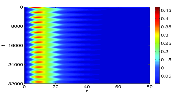
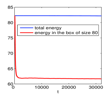
Figure 1: Energy density as a function of position and time (left). Total energy and energy in the box of size $80$ (right).

We display results for $d_{1}=-0.1$, $d_{2}=-3.2$, and $w=12$, although small changes in these parameters give similar results. In the left panel of Figure 1 we show the energy density as a function of $t$ and $r$. A localized, time dependent object is clearly visible. The right panel shows that the initial configuration sheds about a quarter of its energy and quickly settles into the localized oscillon. In the upper left panel of Figure 2 we show the gauge invariant quantity $|\phi(r=0,t)|$. The field is clearly oscillating about the vacuum expectation value at $\phi=1$. The frequency of the oscillation is measured to be $f_{H}=0.2239$. A general characteristic of any long-lived oscillon is that it oscillates at a frequency below the frequency of the modes that can carry energy away Campbell2 . Note that the mass of the Higgs is $m_{H}=\sqrt{2}$, so the lowest frequency of any propagating mode of the Higgs field is $m_{H}/2\pi=0.2251$, which is just above the oscillon frequency. In the upper right panel we show the gauge invariant quantity $f_{01}(r=10,t)$, which is oscillating with a frequency of $f_{W}=0.1120$. The gauge boson mass is $m_{W}=\sqrt{2}/2$, so the lowest frequency of these propagating modes is $m_{W}/2\pi=0.1125$, which is also just above the oscillation frequency. The field $\chi(r,t)$ has the same mass as $f_{01}(r,t)$ and oscillates at the same frequency.

Oscillons are localized in space. Going far from the origin, where we can linearize the theory, for each field we expect to find a relationship of the form $2\pi f=\sqrt{m^{2}-\epsilon^{2}}$, where the fields approach their vacuum values like $\exp(-\epsilon r)$ for large $r$. Unfortunately, the precision with which we can estimate the $\epsilon$ for each field from our numerical data is very limited, so we have only checked that it agrees with the predicted value to within an order of magnitude.

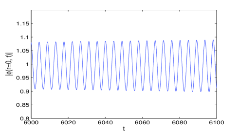
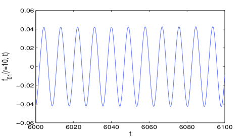
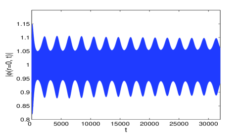
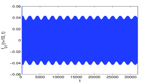
Figure 2: $|\phi(r=0,t)|$ (left) and $f_{01}(r=10,t)$ (right) as functions of time for $d_{1}=-0.1$ and $d_{2}=-3.2$.

In the lower panels of Figure 2 we plot the two fields over a much longer time, so the fundamental oscillations are not visible. On this scale, however, we see beats, at the same frequency in all fields. For this configuration the beat frequency is about $5\times 10^{-4}$, but it can vary substantially in response to variations of the initial parameters.

V Conclusions

In the model we have studied, we have numerically discovered an oscillon that shows no sign of decay after more than 14,000 oscillations. This result suggests that this object is extremely long-lived. If such a similarly long-lived object were to exist in the Standard Model, it would have important phenomenological consequences. It could play a significant role in the dynamics of baryogenesis by providing a mechanism for creating the necessary out-of-equilibrium conditions in the early universe. If this object were extraordinarily long-lived, it could be a dark matter candidate. (A substantial body of work has already investigated such questions for $Q$-balls smallq ; Kasuya ; Enqvist .)

However, a number of questions must be resolved in order to understand the phenomenological implications, if any. Although one might expect objects with spherical symmetry to be energetically favored, it is possible that our oscillon could decay by coupling to nonspherical deformations, which we would not see because of our restriction to the spherical ansatz. Restoring the photon coupling would add another possible decay mechanism. The oscillon could also decay by coupling to fermions, and such decays might be of interest in the early universe. It would be interesting to see if quantum effects modify these conclusions, as they do for small $Q$-balls qball . Finally, and perhaps most importantly, we have only observed oscillons when $m_{H}=2m_{W}$, so it is possible that their unnaturally long lifetime is a consequence of this fine-tuning of parameters in our reduced theory. We imagine that in the full theory, the condition needed for the existence of the oscillon would be slightly modified by the splitting between the $W$ and $Z$ masses. We note that a Higgs mass near $2m_{W}$ is in the middle of the discovery window of the LHC.

VI Acknowledgments

We would like to thank M. Gleiser for turning us on to oscillons. N. G. gratefully acknowledges discussions with P. Forgacs, M. Karliner, N. Manton, O. Schröder, and W. Zakrzewski.

E. F. was supported in part by funds provided by the U.S. Department of Energy (D.O.E.) under cooperative research agreement DE-FC02-94ER40818. N. G. was supported in part by the National Science Foundation through the Vermont Experimental Program to Stimulate Competitive Research (VT-EPSCoR). R. M. was supported by the Undergraduate Research Opportunities Program at the Massachusetts Insitute of Technology.

References

- (1) S. Coleman, Aspects of Symmetry (Cambridge University Press, Cambridge, 1985).
- (2) R. Rajaraman, Solitons and Instantons (North-Holland, Amsterdam, 1982).
- (3) R. F. Dashen, B. Hasslacher, and A. Neveu, Phys. Rev. D11 (1975) 3424.
- (4) S. Coleman, Nucl. Phys. B262 (1985) 263.
- (5) D. K. Campbell, J. F. Schonfeld and C. A. Wingate, Physica 9D, 1 (1983).
- (6) I. L. Bogolubsky and V. G. Makhankov, JETP Lett 24 (1976) 12.
- (7) M. Gleiser, hep-ph/9308279, Phys. Rev. D49 (1994) 2978; E. J. Copeland, M. Gleiser and H. R. Muller, hep-ph/9503217, Phys. Rev. D52 (1995) 1920; A. Adib, M. Gleiser, and C. Almeida, hep-th/0203072, Phys. Rev. D66 (2002) 085011.
- (8) S. Kasuya, M. Kawasaki, and F. Takahashi, Phys. Lett. B559 (2003) 99.
- (9) M. Gleiser, hep-th/0408221, Phys. Lett. B600 (2004) 126.
- (10) B. Piette and W. J. Zakrzewski, Nonlinearity 11 (1998) 1103.
- (11) G. Fodor and I. Racz, Phys. Rev. Lett. 92 (2004) 151801; P. Forgacs and M. S. Volkov, Phys. Rev. Lett. 92 (2004) 151802.
- (12) H. Segur and M. D. Kruskal, Phys. Rev. Lett. 58 (1987) 747.
- (13) J. N. Hormuzdiar and S. D. Hsu, Phys. Rev. C59 (1999) 889.
- (14) E. Farhi, K. Rajagopal, and R. Singleton, hep-ph/9503268, Phys. Rev. D52 (1995) 2394.
- (15) R. F. Dashen, B. Hasslacher, and A. Neveu, Phys. Rev. D10 (1974) 4130; E. Witten, Phys. Rev. Lett. 38 (1977) 121; P. Forgacs and N. S. Manton, Commun. Math. Phys. 72 (1980) 15; B. Ratra and L. G. Yaffe, Phys. Lett. B205 (1988) 57.
- (16) D. K. Campbell, S. Flach, and Y. S. Kivshar, Physics Today 57 (2004) 43.
- (17) A. Kusenko, Phys. Lett. B405 (1997) 285; A. Kusenko, Phys. Lett. B406 (1997) 26; A. Kusenko, Phys. Lett. B418 (1998) 46.
- (18) S. Kasuya and M. Kawasaki, Phys. Rev. D61 (2000) 041301;
- (19) K. Enqvist and J. McDonald, Phys. Lett. B425 (1998) 309; K. Enqvist and J. McDonald, Nucl. Phys. B570 (2000) 407.
- (20) N. Graham, Phys. Lett. B513 (2001) 112.