Quantum effective actions
from nonperturbative worldline dynamics

Abstract

We demonstrate the feasibility of a nonperturbative analysis of quantum field theory in the worldline formalism with the help of an efficient numerical algorithm. In particular, we compute the effective action for a super-renormalizable field theory with cubic scalar interaction in four dimensions in quenched approximation (small-$N_{\text{f}}$ expansion) to all orders in the coupling. We observe that nonperturbative effects exert a strong influence on the infrared behavior, rendering the massless limit well defined in contrast to the perturbative expectation. Our numerical method is based on a direct use of probability distributions for worldline ensembles, preserves all Euclidean spacetime symmetries, and thus represents a new nonperturbative tool for an investigation of continuum quantum field theory.

HD-THEP-05-12, http://arXiv.org/abs/hep-th/0505275

PACS numbers: 11.10.Gh, 11.15.Tk, 12.20.Ds

1 Introduction

Many current problems in particle physics as well as statistical physics demand for new nonperturbative field theoretic techniques. Particularly, the treatment of strongly coupled fluctuations requires methods that go beyond standard perturbative techniques.

Conventionally, perturbation theory is understood as an expansion for both small coupling and small amplitude of the fields. The case of larger fields but small coupling can be addressed with effective-action techniques that take the coupling to all orders to an external field into account; prominent examples are the Heisenberg-Euler effective action [1] or the Coleman-Weinberg effective potential [2].

In the present work, we propose a technique that has the potential to deal with the opposite limit: arbitrary coupling but weak external-field amplitude. The technique is based on the worldline formulation of quantum field theory that goes back to ideas of Feynman [3]; it can be viewed as a mapping of field theoretic problems onto quantum mechanical path integrals, identifying the trajectory of a fluctuation in coordinate space with the path of a quantum mechanical particle. The approach had occurred rarely in the literature, see, e.g., [4], until it was realized that certain perturbative computations simplify tremendously in the worldline approach [5, 6]; the deep reason behind this observation is the fact, that the worldline formulation of field theoretic correlators can be understood as the infinite string-tension limit of string-theory amplitudes, giving rise to a higher level of organization of the expressions. Important progress was made by generalizing the worldline techniques to effective-action computations [7, 8]. By now, the formalism has found a wide range of application, see, for instance, [9, 10, 11, 12, 13, 15, 14, 16, 17, 18]. The power of the worldline approach became particularly apparent in combination with numerical Monte-Carlo techniques [19, 20]; worldline numerics in the form of efficient and fast algorithms is now available for the computation of effective actions or Casimir energies for highly general forms of the external field. For instance, nonlocal phenomena and fluctuation-induced geometry-dependent interactions can now be computed reliably and straightforwardly [21, 22].

The majority of applications of the worldline approach remains perturbative in the coupling, even though formal all-order expressions can already be found in the early works [3]. The present work aims at exploiting these and related formal expressions for a direct evaluation of all-order results by numerical Monte-Carlo means. We demonstrate the potential of worldline numerics for nonperturbative problems with the aid of a super-renormalizable model field theory involving a “charged” real scalar field $\phi$ coupled to a “scalar photon” $A$. Promoting the $\phi$ field formally to an $N_{\text{f}}$-component field, we study the system by means of an expansion for small $N_{\text{f}}$. Already at leading nontrivial order, this expansion corresponds to an infinite set of Feynman diagrams involving one open $\phi$ line or, alternatively, one closed $\phi$ loop but arbitrarily many scalar photon fluctuations. We refer to the leading nontrivial order as the “quenched approximation”. This approximation holds for arbitrarily large values of the coupling. Although it also includes infinitely many couplings to the external field, we expect that the approximation is most reliable for weak field amplitudes. As a first concrete application, we compute the nonperturbative effective action for the scalar photon, $\Gamma[A]$, in the quenched approximation, concentrating on the induced interactions of soft photons. In this way, we obtain an effective action of Heisenberg-Euler type to leading order in $N_{\text{f}}$ but to all orders in the coupling.

The main purpose of the present work is to demonstrate that our method is capable of giving answers to nonperturbative problems with a computation from first principles. With regard to more realistic quantum field theories, our work serves as a feasibility study. Nevertheless, even in the simple model we observe new phenomena that may generalize to other theories as well. Of special relevance is the following result: whereas the perturbative expansion is ill-defined for a massless $\phi$ field (similar, e.g., to massless QED), the nonperturbative effective action remains valid for massless fields, revealing the unexpected breakdown of perturbation theory (and not of the theory itself) in this limit.

Our work is related to other nonperturbative investigations of field theoretic problems based on the worldline approach: in [24], scalar QED (ScQED) in quenched approximation was considered, and an instanton approximation of the path integral was used to compute all-order corrections to the Schwinger pair-production rate in a constant electric field. Furthermore, a comprehensive study of the worldline expressions for various quenched propagators has been performed in [25], employing a variational approach. Therein, the nonperturbatively interacting path integrals are approximated by optimizing a trial action according to a variational principle. In [26], the worldline approach was used to deduce information about the nonperturbative quenched propagator beyond the well-controlled infrared (IR) limit. A combination of Monte-Carlo techniques with the worldline approach has also been used in [27] for the determination of bound-state properties from 4-point correlators; see also [28] for an approach to QCD bound states. Moreover, non perturbative worldline methods have been used to calculate the chiral anomalies [29],[30].

We start the presentation of our work in Sect. 2 by rederiving the worldline expressions for the effective action and the nonperturbative propagator in quenched approximation. Even though the final results are known in the literature, we present their derivation here (with details in App. A) in the modern language of generating functionals of correlation functions using functional integrals. In Sect. 3, we elucidate the numerical algorithm, concentrating on the new aspects introduced by the present work, and presenting results for the free theory as a useful example; another illustrative example is presented in App. C. In Sect. 4, we summarize our main numerical results for the self-interaction potential of the worldlines which lies at the heart of the nonperturbative dynamics. Section 5 employs this numerical data to derive our main result, the effective action of the scalar photon. We explain how the standard renormalization procedure applies to the present nonperturbative study. Section 6 summarizes our conclusions and gives an outlook.

2 Nonperturbative worldline methods in QFT

Let us consider a specific Euclidean quantum field theoretic model in $D$ dimensional spacetime involving two interacting real scalar fields $\phi$ and $A$ with bare Lagrangian

$$\mathcal{L}(\phi,A)=\frac{1}{2}(\partial_{\mu}\phi)^{2}+\frac{1}{2}m^{2}\phi^{2}+\frac{1}{2}(\partial_{\mu}A)^{2}-\frac{\text{i}}{2}\,h\,A\phi^{2}.$$ (1)

This model meets our requirements in many respects: (i) it has a well-defined perturbative expansion, (ii) it will turn out to have also a well-defined nonperturbative expansion in the quenched approximation, (iii) the interaction $\sim hA\phi^{2}$ is super-renormalizable in $D=4$, since the coupling has positive mass dimension $[h]=1$, and hence facilitates a simple analysis of the (nonperturbative) divergencies, (iv) the imaginary interaction imitates the interaction occurring in QED with $A$ being the scalar analogue of the massless photon field; hence, $A$ will be called the “scalar photon” in the following. We are well aware of the fact that this Lagrangian does not define a fully consistent QFT, since the potential is not bounded from below; however, contrary to the corresponding model with a real interaction (the Wick-Cutkosky model), the present model does not have propagator singularities which would signal the metastability of the model immediately and require a careful treatment. Nevertheless, the Euclidean effective action will turn out to exhibit nonzero imaginary parts which suggest a relation to decay widths of the metastable states. Note that in [31] it was argued that, despite the obvious non-hermiticity of the Hamiltonian of this model, the spectrum could be positive definite by virtue of a careful implementation of PT symmetry.

Let us first concentrate on the effective action $\Gamma[A]$ for soft scalar photons with momenta $p^{2}$ smaller than the scale of the massive $\phi$ field, $p^{2}\ll m^{2}$. This effective action can be derived from the Schwinger functional,

$$Z[J]\equiv e^{W[J]} = \int\mathcal{D}\hat{A}\mathcal{D}\phi\,e^{-\int_{x}\mathcal{L}(\phi,\hat{A})+\int_{x}J\hat{A}}$$ (2)

$$= \int\mathcal{D}\hat{A}\,\det{}^{-1/2}\big{(}-\partial^{2}+m^{2}+\text{i}h\hat{A}\big{)}\,e^{-\int_{x}\frac{1}{2}(\partial_{\mu}\hat{A})^{2}+\int_{x}J\hat{A}}$$

$$= \int\mathcal{D}\hat{A}\,e^{-S_{\text{eff}}(\hat{A})+\int_{x}J\hat{A}},$$

where $\int_{x}\equiv\int d^{D}x$ and $S_{\text{eff}}$ denotes an auxiliary effective action governing the quantum dynamics of the scalar photon (it should not be confused with the full quantum effective action $\Gamma[A]$ defined below). Here, we have integrated out the massive $\phi$ field, resulting in a functional determinant that can be displayed in worldline form:

$$S_{\text{eff}}(\hat{A}) = \int_{x}\frac{1}{2}(\partial_{\mu}\hat{A})^{2}+\frac{1}{2}\ln\det\big{(}-\partial^{2}+m^{2}+\text{i}h\hat{A}\big{)}$$ (3)

$$= \int_{x}\frac{1}{2}(\partial_{\mu}\hat{A})^{2}-\frac{1}{2}\int_{0}^{\infty}\frac{dT}{T}\,e^{-m^{2}T}\,\,\text{Tr}\,e^{(-\partial^{2}+\text{i}h\hat{A})}$$

$$= \int_{x}\frac{1}{2}(\partial_{\mu}\hat{A})^{2}-\frac{1}{2(4\pi)^{D/2}}\int_{0}^{\infty}\frac{dT}{T^{1+D/2}}\,e^{-m^{2}T}\Big{\langle}e^{\text{i}h\int_{0}^{T}d\tau\,\hat{A}(x(\tau))}\Big{\rangle}_{x}.$$

Here, the expression $\langle\dots\rangle_{x}$ denotes an expectation value with respect to an ensemble of worldlines $x(\tau)$ with a Gaußian velocity distribution,

$$\langle\dots\rangle_{x}=\frac{\int\mathcal{D}x\,\dots\,e^{-\frac{1}{4}\int_{0}^{T}d\tau\,\dot{x}^{2}}}{\int\mathcal{D}x\,e^{-\frac{1}{4}\int_{0}^{T}d\tau\,\dot{x}^{2}}}.$$ (4)

In a standard fashion, the effective action $\Gamma[A]$ – the generating functional of all 1PI correlation functions of the scalar photons – is related to the Schwinger functional by a Legendre transformation,

$$\Gamma[A]=-W[J]+\int_{x}JA,$$ (5)

with $J=J[A]$ being a functional of the “classical” field $A$ (conjugate to the source $J$) defined by

$$A(x):=\frac{\delta W[J]}{\delta J(x)}\equiv A[J].$$ (6)

In this work, we will evaluate $\Gamma[A]$ in the so-called quenched approximation. In a diagrammatic language, the quenched approximation for $\Gamma[A]$ can be characterized by taking into account all diagrams with exactly one closed $\phi$ loop, but arbitrarily many virtual scalar photon fluctuations, see Fig. 1. From a different viewpoint, the quenched approximation would correspond to the lowest nontrivial order in an $N_{\text{f}}$ expansion if we promoted the $\phi$ field to have $N_{\text{f}}$ components.

Figure 1: Diagrams included in the quenched approximation.

More formally, let us introduce the $\phi$ field worldline current

$$j(x):=\text{i}h\int d\tau\,\delta^{(D)}(x-x(\tau)),$$ (7)

such that the interaction of the scalar photon $A$ with the $\phi$ worldline can be expressed as

$$\Big{\langle}e^{\text{i}h\int_{0}^{T}d\tau\,A(x(\tau))}\Big{\rangle}_{x}=\Big{\langle}e^{\int_{x}jA}\Big{\rangle}_{x}.$$ (8)

Then the quenched approximation consists in dropping all terms involving worldline correlators between two different $j$ currents of the $\phi$ field, $\mathcal{O}(\langle j_{1}\dots j_{2}\rangle_{x_{1},x_{2}})\to 0$. Since each current couples to all orders to the classical field $A$, we expect this approximation to be good if the scalar photon field under consideration is weak compared to other mass scales of the system. Nevertheless, the quenched approximation does not restrict the value of the coupling $h$ which therefore can be arbitrarily large.

In appendix A, we derive the general worldline representation of the Schwinger functional and perform the Legendre transform yielding the effective action. In the quenched approximation, $\Gamma[A]$ can be displayed in closed form (cf. Eq. (75)),

$$\Gamma_{\text{QA}}[A]=\int_{x}\frac{1}{2}(\partial_{\mu}A)^{2}-\frac{1}{2(4\pi)^{D/2}}\int_{0}^{T}\frac{dT}{T^{1+D/2}}\,e^{-m^{2}T}\Big{\langle}e^{\frac{1}{2}\int_{x}j\Delta j+\int_{x}jA}\Big{\rangle}_{x},$$ (9)

where $\Delta=1/(-\partial^{2})$ denotes the propagator of the scalar photon with coordinate space representation

$$\Delta(x_{1},x_{2})=\frac{\Gamma\left(\frac{D-2}{2}\right)}{4\pi^{D/2}}\,\frac{1}{|x_{1}-x_{2}|^{D-2}}.$$ (10)

It is important to note that, in particular, all contributions from the scalar photon fluctuations are summarized in the exponential with a worldline current-current interaction $\sim\int_{x}j\Delta j$. Re-expressed in terms of the worldline coordinates $x(\tau)$ of the $\phi$ field fluctuations, this term acts like a self-interaction potential $V[x]$ of the worldline,

$$\frac{1}{2}\int_{x}j\Delta j = -\frac{h^{2}}{8\pi^{D/2}}\,\Gamma\left({\scriptstyle\frac{D-2}{2}}\right)\int_{0}^{T}d\tau_{1}d\tau_{2}\,\frac{1}{|x_{1}-x_{2}|^{D-2}}$$ (11)

$$=: -g\,V[x],\quad\text{with}\,\,g:=\frac{h^{2}}{8\pi^{D/2}}\,\Gamma\left({\scriptstyle\frac{D-2}{2}}\right).$$

Here, we have introduced an effective coupling $g$ for convenience. Therefore, a thorough analysis of the properties of this potential and its vacuum expectation value is mandatory for an understanding of the nonperturbative dynamics. This is one of the main aims of the present work. In addition to the effective action for the scalar photon, also proper vertices with external $\phi$ lines can be studied nonperturbatively on the worldline. In particular, the computation of the propagator of the $\phi$ field is straightforward and its worldline representation can be compactly written as

$$G(x_{\text{F}},x_{\text{I}})=\frac{1}{(4\pi)^{D/2}}\int_{0}^{\infty}\frac{dT}{T^{D/2}}\,e^{-m^{2}T}\,e^{-\frac{|x_{\text{F}}-x_{\text{I}}|^{2}}{4T}}\,\Big{\langle}e^{-gV[x]}\Big{\rangle}_{x_{\text{I}}}^{x_{\text{F}}}.$$ (12)

Here, the expectation value $\langle\dots\rangle_{x_{\text{I}}}^{x_{\text{F}}}$ implies that we are dealing with open worldlines ranging from $x_{\text{I}}$ to $x_{\text{F}}$. Again a proper understanding of the properties of the potential term is required.

Furthermore, we would like to point out that the $\phi$ propagator can even be generalized to the case of arbitrarily many couplings to an external scalar photon background $A$ by including a factor of $e^{\text{i}g\int_{0}^{T}d\tau A(x(\tau))}$ in the expectation value of Eq. (12).

Let us conclude this section by translating the present results to scalar quantum electrodynamics (ScQED). In this case, the bare Lagrangian is given by

$$\mathcal{L}_{\text{ScQED}}=|D_{\mu}[A]\phi|^{2}+m^{2}|\phi|^{2}+\frac{1}{4}F_{\mu\nu}F_{\mu\nu},$$ (13)

where $\phi$ now denotes a complex scalar field and $D_{\mu}[A]=\partial_{\mu}+\text{i}eA_{\mu}$ is the covariant derivative. Most of our formulas can immediately be generalized to this case with the effective photon action given by

$$\Gamma_{\text{QA}}[A_{\mu}]=\int_{x}\frac{1}{4}F_{\mu\nu}F_{\mu\nu}-\frac{1}{(4\pi)^{D/2}}\int_{0}^{\infty}\frac{dT}{T^{1+D/2}}\Big{\langle}e^{\frac{1}{2}\int_{x}j_{\mu}\Delta_{\mu\nu}j_{\nu}+\int_{x}j_{\mu}A_{\mu}}\Big{\rangle}_{x},$$ (14)

with the worldline current of the charged field

$$j_{\mu}(x)=\text{i}e\int_{0}^{T}d\tau\,\dot{x}_{\mu}(\tau)\,\delta^{(D)}(x-x(\tau)),$$ (15)

and the photon propagator

$$\Delta_{\mu\nu}(x_{1},x_{2}) = \frac{\Gamma(\frac{D-2}{2})}{4\pi^{D/2}}\left[\frac{1+\alpha}{2}\frac{1}{|x_{1}-x_{2}|^{D-2}}+({\scriptstyle\frac{D}{2}}-1)(1-\alpha)\frac{(x_{1}-x_{2})_{\mu}(x_{1}-x_{2})_{\nu}}{|x_{1}-x_{2}|^{D}}\right],$$ (16)

with gauge parameter $\alpha$. The interaction between the charged worldline current and the photon field then occurs in the form of a Wegner-Wilson loop,

$$e^{\int_{x}j_{\mu}A_{\mu}}=e^{\text{i}e\oint dx_{\mu}A_{\mu}(x)}.$$ (17)

Here, the current-current interaction induced by the virtual photon exchanges inside the $\phi$ loop now implies a worldline self-interaction potential of the form

$$\frac{1}{2}\int_{x}j_{\mu}\Delta_{\mu\nu}j_{\nu}=-\frac{e^{2}}{8\pi^{D/2}}\Gamma({\scriptstyle\frac{D-2}{2}})V_{\text{ScQED}}[x]$$ (18)

with

$$V_{\text{ScQED}}[x]=\int_{0}^{T}d\tau_{1}d\tau_{2}\,\left[\frac{1+\alpha}{2}\frac{\dot{x}_{1}\cdot\dot{x}_{2}}{|x_{1}-x_{2}|^{D-2}}+({\scriptstyle\frac{D}{2}}-1)(1-\alpha)\frac{\dot{x}_{1}\cdot(x_{1}-x_{2})(x_{1}-x_{2})\cdot\dot{x}_{2}}{|x_{1}-x_{2}|^{D}}\right].$$ (19)

Note that the second term drops out completely in the Feynman gauge with $\alpha=1$. In fact, all $\alpha$-dependent terms can be shown to correspond to a total derivative that automatically vanishes in the case of the photon effective action where all worldlines are closed loops [8].

The representation of the scalar propagator in Eq. (12) does also hold in the case of ScQED with $V[x]$ replaced by $V_{\text{ScQED}}[x]$ of Eq. (19) and $g_{\text{ScQED}}=\frac{e^{2}}{8\pi^{D/2}}\Gamma({\scriptstyle\frac{D-2}{2}})$.

In the case of ordinary spinor QED, an additional complication arises from the coupling between fermionic spin and the electromagnetic field. Using a convenient spin-factor representation, the present formulation can be shown to hold with the simple insertion of the spin factor in all worldline expectation values, see [32], [33].

3 Worldline numerics

In this section, we develop the discretization of the integral in the proper time. Since the discretization is done for an auxiliary variable, i.e., an integration parameter, it has the advantage of preserving the continuum spacetime symmetries, i.e., the Lorentz (Euclidean) invariance. Also gauge and chiral symmetries would be preserved if present. This is the major difference between nonperturbative worldline numerics and other Monte-Carlo methods such as lattice field theory. In this sense, our method is much closer to analytic continuum field-theory techniques than to numerical lattice formulations.

3.1 Algorithmic principles

In this work, we evaluate the worldline integrals, corresponding to quantum mechanical path integrals, by means of Monte-Carlo algorithms, as proposed for perturbative amplitudes in [19]. For this, we approximate the infinite set of worldlines by a finite ensemble with $n_{\text{L}}$ configurations. Furthermore, we discretize the propertime parameter of each worldline, such that the fluctuating worldline is specified by a set of $N$ points per line (ppl),

$$\langle\dots\rangle_{x} = \frac{\int\mathcal{D}x\dots P[x]}{\int\mathcal{D}xP[x]}\,\to\frac{1}{n_{\text{L}}}\sum_{\{x\}}\dots,\quad\text{with}\quad P[x]=e^{-\frac{1}{4}\int_{0}^{T}d\tau\dot{x}^{2}},$$

$$x(\tau) \to x_{i}\in\mathbbm{R}^{D},\quad i=0,1,\dots,N.$$ (20)

In the case of the effective action, the worldlines form closed loops and we identify $x_{0}$ with $x_{N}$; in the case of the $\phi$ propagator, where the initial and final point of the worldline are fixed, we use the definition $x_{0}=x_{\text{I}}$ and $x_{N+1}=x_{\text{F}}$.

The finite number of worldlines $n_{\text{L}}$ introduces a statistical error that will be estimated automatically by the Monte-Carlo algorithm. The finite number of points per worldline $N$ implies a systematic error that has to be analyzed straightforwardly by approaching the propertime continuum limit $N\to\infty$. This is the most sumptuous point of the present investigation.

An immediate realization of Eq. (20) requires to generate a different ensemble for each value of the propertime parameter $T$, occurring in the Gaußian velocity distribution. This can elegantly be circumvented by introducing unit loops or lines $y(t)$ [19],

$$y(t):=\frac{1}{\sqrt{T}}\,x(Tt),\quad t\in[0,1],$$ (21)

such that the velocity distribution for $y(t)$ becomes independent of $T$,

$$\int_{0}^{T}d\tau\,\dot{x}^{2}(\tau)=\int_{0}^{1}dt\,\dot{y}^{2}(t).$$ (22)

Here, the dot always denotes a derivative with respect to the corresponding argument. As a consequence, one and the same ensemble of unit loops or lines can be used for all values of $T$, saving an enormous amount of CPU time. Of course, this change of variables also affects the remaining worldline integrand, for instance, the self-interaction potential,

$$V[x] = \int_{0}^{T}d\tau_{1}d\tau_{2}\,\frac{1}{|x_{1}-x_{2}|^{D-2}}=T^{3-D/2}\,\int_{0}^{1}dt_{1}dt_{2}\,\frac{1}{|y_{1}-y_{2}|^{D-2}},$$ (23)

$$=: T^{3-D/2}\,v[y]$$

where we have introduced the dimensionless self-interaction potential of the unit loops, $v[y]$. For computations of the $\phi$ propagator, the variable transformation also affects the boundary points, inducing a further $T$ dependence, $x_{\text{F}}=\sqrt{T}y_{\text{F}}$, $x_{\text{I}}=\sqrt{T}y_{\text{I}}$, that can nevertheless be handled straightforwardly.

In the context of the effective-action calculation involving closed worldlines, one final convenient step for the algorithm consists in using the center-of-mass decomposition of the worldlines, $x(Tt)=x_{\text{CM}}+\sqrt{T}y(t)$, such that the unit loops satisfy $\int_{0}^{1}dt\,y(t)=0$. This implies that the ensemble average becomes

$$\langle\mathcal{F}[x]\rangle_{x}=\int d^{D}x_{\text{CM}}\,\langle\mathcal{F}[x_{\text{CM}}+\sqrt{T}y]\rangle_{y}.$$ (24)

This allows to study the effective action density, i.e., the effective Lagrangian, locally, with the center-of-mass integration corresponding to the usual relation between action and Lagrangian, $\Gamma=\int d^{D}x_{\text{CM}}\mathcal{L}$.

For the Monte-Carlo generation of the worldline ensembles, there are various efficient techniques available that do not require to spend computer time on dummy thermalization sweeps, as it would be the case for standard heat-bath algorithms. Fast algorithms are, for instance, the Fourier loop algorithm, “f loops”, or explicit diagonalization of the velocity distribution, “v loops”, see [22]. For most computations in the present work, we use a new algorithm that is based on a point doubling procedure (“d loops” and “d lines”) that is described in appendix B.

Beyond these general algorithmic aspects, we encounter a particular numerical problem in the present case upon discretizing the self-interaction potential (23): the integrand for coinciding points $y_{1}=y_{2}$ is ill-defined. The possibly arising divergence can be viewed as a “self-energy” of the worldline. We regularize the discretized sum by taking out the coincident points by hand,

$$v[y]\to\frac{1}{N^{2}}\sum_{i\neq j}\frac{1}{|y_{i}-y_{j}|^{D-2}},\quad,i,j=0,\dots N.$$ (25)

A singular behavior of the original integral then manifests itself in a strong $N$ dependence of $v[y]$ which we will carefully control. Since the distance of the nearest-neighbor points decreases for increasing $N$, $|y_{i}-y_{i+1}|\sim 1/\sqrt{N}$, such strong $N$ dependence signals a short-distance UV singularity that will be subject to renormalization of physical parameters. Alternatively, we could include the coincident points in the above sum by shifting the denominator, $|y_{i}-y_{j}|\to|y_{i}-y_{j}|+\epsilon$, and study the limiting behavior with $\epsilon\to 0$. However, since the latter limit will always interfere numerically with the large-$N$ limit (which has to be taken anyway), the first proposed method can be handled more straightforwardly.

3.2 Free theory

As a first useful application, let us study the worldline representation for the free theory in the limit of vanishing interaction, e.g., $h\to 0$ for the purely scalar system. An instructive example is given by the kinetic action for the worldlines, $S_{\text{w}}$, characterizing the Gaußian probability distribution of the worldline ensemble,

$$P[x]=\bar{\cal N}\exp(-S_{\text{w}}[x]),$$ (26)

where $\bar{\cal N}$ is the normalization, ensuring $\int\mathcal{D}x\,P[x]$=1. Discretizing the free worldline action $S_{\text{w}}$ (introduced in Eq. (4)), as outlined above for the case of the $\phi$ propagator, we obtain

$$S_{\text{w}}=\frac{1}{4}\int_{0}^{T}d\tau\dot{x}^{2}(\tau)\to\frac{N+1}{4T}\sum_{i=1}^{N+1}(x_{i}-x_{i-1})^{2},$$ (27)

with $x_{0}=x_{\text{I}}$ and $x_{N+1}=x_{\text{F}}$ the corresponding initial and final points of the $\phi$ propagation. For the propagator, we would finally have to integrate over the propertime $T$. However, we will be satisfied here with the propertime integrand and set $T$ to some fixed value in the following.

The ensemble average and the value of the root mean square (RMS) of the free worldline action can be calculated analytically. For this, let us consider the auxiliary integral

$$I_{N}(x_{\text{F}},x_{\text{I}},T,\kappa)=\int dx_{1}\cdots dx_{N}\exp\{-\frac{\kappa\Delta\tau}{4}\sum_{i=1}^{N+1}\frac{(x_{i}-x_{i-1})^{2}}{\Delta\tau^{2}}\},$$ (28)

where $\Delta\tau=T/(N+1)$, and we have suppressed the Lorentz indices of the $x_{i}$’s which are points in $D$ dimensional spacetime. The parameter $\kappa$ is arbitrary here which will be exploited below.

The integral is Gaußian and can be done exactly. We rewrite the integral as

$$I_{N}(x_{\text{F}},x_{\text{I}},T,\kappa)=\int dx_{1}\cdots dx_{N}\exp\{-\frac{\kappa\Delta\tau}{4}\frac{1}{\Delta\tau^{2}}(x_{\text{I}}^{2}+x_{\text{F}}^{2}-2x_{\text{I}}x_{1}-2x_{\text{F}}x_{N}+x_{i}A_{ij}x_{j})\},$$ (29)

where $A$ is a symmetric matrix,

$$A_{ij}=2\delta_{ij}-\delta_{i+1,j}-\delta_{i,j+1},\quad i,j=1,\dots,N.$$ (30)

Introducing the auxiliary current $\eta_{i}$,

$$\eta_{i}=-2x_{\text{I}}\delta_{i1}-2x_{\text{F}}\delta_{iN},$$ (31)

the integral reads

$$I_{N}(x_{\text{F}},x_{\text{I}},T,\kappa)=(\frac{4\pi\Delta\tau}{\kappa})^{\frac{ND}{2}}\frac{1}{\sqrt{\det(A)}^{D}}\exp\left[\frac{\kappa}{4\Delta\tau}\frac{\eta_{i}(A^{-1})_{ij}\eta_{j}}{4}-\frac{\kappa}{4\Delta\tau}(x_{\text{I}}^{2}+x_{\text{F}}^{2})\right],$$ (32)

with

$$\eta_{i}(A^{-1})_{ij}\eta_{j}=4(x_{\text{I}}^{2}(A^{-1})_{11}+2x_{\text{I}}x_{\text{F}}(A^{-1})_{1N}+A^{-1}_{NN}x_{\text{F}}^{2}).$$ (33)

The ensemble average of the free action can now be calculated from the auxiliary integral,

$$\langle S_{\text{w}}\rangle=\bar{\cal N}\int dx_{1}\cdots dx_{N}\;S_{\text{w}}\;\exp\{-S_{\text{w}}\}=\bar{\cal N}\int dx_{1}\cdots dx_{N}\;\frac{-d}{d\kappa}\;\exp\{-\kappa S_{w}\}\bigg{|}_{\kappa=1}.$$ (34)

The integral actually agrees with $I_{N}$ of Eq. (32) above, therefore

$$\langle S_{\text{w}}\rangle = \bar{\cal N}\;\frac{-d}{d\kappa}\left(\frac{4\pi\Delta\tau}{\kappa}\right)^{\frac{ND}{2}}\frac{1}{(\sqrt{\det A})^{D}}\exp\{-\frac{\kappa}{4T}(x_{\text{F}}-x_{\text{I}})^{2}\}\bigg{|}_{\kappa=1}$$ (35)

$$= \frac{1}{2}N\,D+\frac{1}{4T}(x_{\text{F}}-x_{\text{I}})^{2}.$$

Notice that the result corresponds to the classical action plus one half times the number of degrees of freedom.

In table 1, we show a comparison between the exact results and those of the numerical calculation using our Monte-Carlo code for different parameters. The numerical result is always very satisfactory with a precision better than 0.1 % in all cases. This illustrates the power of the Monte-Carlo method.

$N$	$2T$	$x_{\text{F}}$	$\langle S_{\text{w}}\rangle_{\rm numerical}$	$\langle S_{\text{w}}\rangle_{\rm theory}$	$\Delta S_{\text{w}}/S_{\text{w}}(\%)$
31	0.5	(10,0,10,0)	161.895	162	-0.06
1023	0.5	(0,0,0,0)	2046.38	2046	0.02
1023	0.5	(10,0,0,0)	2096.00	2096	0.00
4095	0.5	(0,0,0,0)	8190.15	8190	0.001
4095	0.5	(10,0,0,0)	8238.70	8240	-0.02
4095	0.5	(100,0,0,0)	13189.4	13190	-0.005

Table 1: Average theoretical and numerical actions. All numerical calculations were done with $n_{\text{L}}=10^{4}$ worldlines. We have set $D=4$ and $x_{\text{I}}=(0,0,0,0)$.

We underline a fact that will be of the outmost importance in the more involved non perturbative calculation below, namely that the Monte-Carlo method also provides information about the probability distribution of the free action itself. For instance, the probability of finding a configuration with worldline action $S_{\text{w}}^{\prime}$ is given by

$${\cal P}(S_{\text{w}}^{\prime})=\bar{\mathcal{N}}\int dx_{1}\cdots dx_{N}\,\delta(S_{\text{w}}-S_{\text{w}}^{\prime})\,\exp\{-S_{\text{w}}\},$$ (36)

which can be evaluated analytically, yielding

$${\cal P}(S_{\text{w}}^{\prime})=\bar{\cal N}(S_{\text{w}}^{\prime}-S_{\rm class})^{-1+\frac{ND}{2}}e^{-(S_{\text{w}}^{\prime}-S_{\rm class})}\;\theta(S_{\text{w}}^{\prime}-S_{\rm class}),$$ (37)

where $S_{\rm class}=(1/4T)(x_{\text{F}}-x_{\text{I}})^{2}$ is the classical action. In Fig. 2, we compare the action distribution calculated with our Monte-Carlo code to the analytical result. The agreement with the theoretical calculation is excellent.

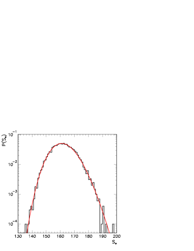
Figure 2: Action distribution from the Monte-Carlo method (histogram) in comparison with the analytical calculation (continuous line) for $N=31$ and $x_{\text{F}}=(10,0,10,0)$.

Using the probability distribution ${\cal P}(S_{\text{w}}^{\prime})$, it is straightforward to calculate the ensemble average, the RMS, and higher moments of the free action. The ensemble average immediately verifies Eq. (35), whereas the RMS results in

$$\sigma^{2}(S_{\text{w}})=\langle S_{\text{w}}^{2}\rangle-\langle S_{\text{w}}\rangle^{2}=\frac{ND}{2}.$$ (38)

As $N$ increases, the ensemble average $S_{\text{w}}(x_{\text{F}},x_{\text{I}})$ grows as well, and the distribution of $S_{\text{w}}$ broadens. For large $N$, we observe from

$$\frac{\sigma(S_{\text{w}})}{\langle S_{\text{w}}\rangle}\rightarrow\frac{1}{\sqrt{ND/2}}$$ (39)

that the relative width of the distribution becomes narrower.

4 Self-interaction potential in the scalar model

In this section, we perform a detailed numerical analysis of the self-interaction potential, occurring in Eq. (11). In particular, we consider its dimensionless form $v[y]$ defined in Eq. (23) in its discretized regularized version,

$$v[y]=\frac{1}{N^{2}}\sum_{i\neq j}\frac{1}{|y_{i}-y_{j}|^{D-2}},$$ (40)

as discussed in Eq. (25). In the following, we concentrate on $D=4$ dimensional spacetime. Other dimensions can be treated in the same way.

The average value of the self-interaction potential $v[y]$ as a function of the number of points per loop can be seen in Fig. 3 together with a logarithmic fit. Obviously, the self-interaction potential diverges logarithmically with $N$,

$$\langle v\rangle_{y}=a+b\ln(N),$$ (41)

with $a\simeq 0.363$ and $b\simeq 0.341$. By contrast, the RMS is finite, as is visible in Fig. 4. We have furthermore collected numerical evidence that all the higher-order moments are also finite.

Figure 3: Average value of the self-interaction potential as a function of the logarithmic of the number of points per loop ($N$).

Figure 4: RMS of the scalar to scalar potential as a function of the number of points per loop ($N$).

In order to evaluate ensemble averages, it will become useful to study the distribution of the self-interaction potential defined by

$$P(v)=\hat{\cal N}\int{\cal D}y\;\delta(v-v[y])\;\exp(-S_{\text{w}}[y]-v[y]),$$ (42)

where the normalization is fixed such that $\int dv\,P(v)=1$. We depict the numerical result for this distribution in Fig. 5 with binned values of the potential for two worldline ensembles with different $N$ ppl. The distributions are shifted along the $x$ axis by the logarithmically divergent ensemble average of $v$, but are not modified otherwise. As a result, all the distributions are equal within the numerical accuracy for different values of $N$, demonstrating that all other properties of the distribution are devoid of further divergencies.

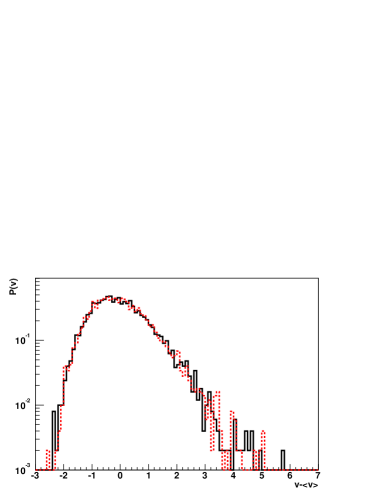
Figure 5: Distribution of potentials for $N=2^{9}$ (continuous line) and $N=2^{12}$ (dashed line). The average values of the distributions have been shifted to lie on top of each other.

This remarkable property reflects the fact that we are dealing with a super-renormalizable interaction. In a diagrammatic language, only a finite subset of diagrams is superficially divergent. In the present scalar model, this finite subset consists of the one-loop contribution to the $\phi$ 2-point function (mass operator), the one- and two-loop scalar photon tadpole and the photon 2-point function (“vacuum polarization”). Once these diagrams are controlled by adjusting the counterterms and renormalizing the corresponding physical parameters, all higher-loop diagrams do not contribute independently to further renormalization; divergencies in subdiagrams will be canceled by the already adjusted counterterms. Evidently, our nonperturbative evaluation of the infinite set of diagrams contributing to the quenched approximation will also benefit from the simplified renormalization in this particular scalar theory.

Let us show that all the characteristics of the average potential can be understood in terms of the distribution of chord distances and that this distribution gives an intuitive picture of the problem.

Figure 6: Chord-distance distribution between pair of points in paths for several values of points per loop, as marked.

For a large number of points per loop we can introduce the chord-distance distribution,

$$v[y]=\frac{1}{N^{2}}\sum_{i\neq j}\frac{1}{l_{ij}^{2}}=\int dl\,p(l)\frac{1}{l^{2}},$$ (43)

where $l_{ij}=|y_{i}-y_{j}|$ abbreviates the chord distances and $p(l)$ is the probability of having two points separated by a distance $l$.

In Fig. 6, we show the chord-distance distribution in a double-log plot for $N=2^{5},2^{12}$, and $2^{14}$. From the figure, we can see that very large chord distances are exponentially suppressed. For very small values of the distance, $l\ll 1/\sqrt{N}$, much less than a typical random step, we see that the probability goes like $l^{D-1}$ which is simply a measure of the available volume in $D$ dimensions. This behavior is a direct consequence of the worldline discretization, and the corresponding branch vanishes in the continuum limit. For intermediate distances the distribution goes like $l^{1}$ which implies that the path spans a 2 dimensional surface, characteristic of a random walk. The contribution to the average potential of the very low chord-distance region is finite, in 4 dimensions. However the intermediate region gives a contribution of order

$$\int_{1/\sqrt{N}}dl\,p(l)\frac{1}{l^{2}}\sim-\ln(1/\sqrt{N}),$$ (44)

which diverges in the continuum limit and gives rise to divergencies in the average potential and, consequently, in the effective action. The divergent part of the average potential carries information about the topological properties of the paths which contribute to the average.

5 Effective action for the scalar photon

Let us now exploit our knowledge about the worldline self-interaction potential in the scalar model in order to compute the nonperturbative effective action $\Gamma[A]$ of the scalar photon in quenched approximation in $D=4$ spacetime dimensions. In this section, we demonstrate how the renormalization procedure can be carried out to all orders, using this example. For this, we need to consider the properties of the potential $V[x]$ for closed worldlines, or its dimensionless counterpart for unit loops, $v[y]$, cf. Eq. (23).

In addition to the quenched approximation, we confine ourselves to slowly varying photon fields with frequencies smaller than the $\phi$ mass scale, $\omega^{2}\ll m^{2}$, for which $A$ can be assumed constant in spacetime. Compared to QED, these assumptions are reminiscent to those leading to the famous Heisenberg-Euler effective action. Notice that this approximation is consistent with the quenched approximation.

Employing the representation (9) together with Eq. (11) and the unit-loop transformation of Eqs. (21)-(23), the effective action in these limits reads in $D=4$,

$$\Gamma_{\text{QA}}[A]=-\frac{1}{32\pi^{2}}\int_{0}^{T}\frac{dT}{T^{3}}\,e^{-m^{2}T}e^{\text{i}hAT}\,\Big{\langle}e^{-gv[y]T}\Big{\rangle}_{y},$$ (45)

where we have taken the photon field dependence out of the worldline average, owing to the $A=$const. assumption.

We make use of the potential distribution, as introduced in the previous section, since it is sufficient for evaluating the nonperturbative effective action of the scalar photon and performing the renormalization program. Let us illustrate this statement with the aid of a simplified fit to the potential distribution; a better but more complex fit will be presented below. As a simplified parameterization of the potential distribution, let us consider

$$P(v)=\frac{\beta^{1+\alpha}}{\Gamma(\alpha+1)}\,(v-v_{0})^{\alpha}\,\exp(-\beta(v-v_{0}))\,\theta(v-v_{0}),$$ (46)

where $\alpha,\beta$ and $v_{0}$ denote fit parameters and $\theta$ is the step function. This distribution is already normalized, $\int dv\,P(v)=1$. Numerically, we find that $\alpha$ and $\beta$ are finite, $\alpha\simeq 0.79$ and $\beta\simeq 13.2$. Only $v_{0}$ diverges with the number of points per loop, which can be related to the divergence of the potential ensemble average, since

$$<v>_{y}=\int dv\;v\;P(v)=v_{0}+\frac{1+\alpha}{\beta}.$$ (47)

With regard to our result of Eq. (41), this implies that

$$v_{0}=b\ln N+a-\frac{1+\alpha}{\beta}\simeq 0.34\,\ln N+0.23\,.$$ (48)

Most importantly, the distribution also provides us with a numerical result for the exponential of the potential, carrying the nonperturbative information about the infinite set of quenched diagrams,

$$\langle e^{-gT\,v[y]}\rangle_{y} = \int dv\,P(v)\,e^{-gTv}$$ (49)

$$= \left(\frac{\beta}{\beta+gT}\right)^{1+\alpha}\,e^{-gTv_{0}}\equiv F_{(\alpha\beta)}(gT)\,e^{-gTv_{0}}.$$

For later convenience, we have introduced the auxiliary function

$$\quad F_{(\alpha\beta)}(x)=\left(\frac{\beta}{\beta+x}\right)^{1+\alpha}.$$ (50)

Inserting this result into Eq. (45), we obtain the numerical estimate for the unrenormalized effective action,

$$\Gamma_{\text{QA}}[A]=-\frac{1}{32\pi^{2}}\int d^{4}x\int_{0}^{T}\frac{dT}{T^{3}}\,e^{-m^{2}T}e^{\text{i}hAT}\,F_{(\alpha\beta)}(gT)\,e^{-gTv_{0}},\quad g=\frac{h^{2}}{8\pi^{2}}.$$ (51)

As for the scalar-photon operators, we demand the renormalization conditions (independently of the approximations)

$$\frac{\delta\Gamma[A=0]}{\delta A(x)}=0,\quad\frac{\delta^{2}\Gamma[A=0]}{\delta A(-p)\delta A(p)}\bigg{|}_{p^{2}=0}=0.$$ (52)

The first condition implements the “no-tadpole” renormalization prescription, whereas the second condition defines the scalar photon to be massless. In general, a third condition fixing the wave function renormalization of the scalar photon $Z_{A}$ has to be implemented; however, it is a peculiarity of the present model that the renormalization shift of this $Z_{A}$ factor remains zero $\delta Z_{A}=0$. Incidentally, the same is true for the wave function renormalization of the $\phi$ field.

These renormalization conditions fix the corresponding counterterms, resulting in the following (partially renormalized) effective action:

$$\Gamma_{\text{QA}}[A]=-\frac{1}{32\pi^{2}}\int d^{4}x\,\int_{0}^{T}\frac{dT}{T^{3}}\,e^{-m^{2}T}\left(e^{\text{i}hAT}-1-\text{i}hAT+\frac{(hAT)^{2}}{2}\right)\,F_{(\alpha\beta)}(gT)\,e^{-gTv_{0}},$$ (53)

where we have also subtracted the zero-point energy, enforcing $\Gamma[A=0]=0$. Note that these renormalization conditions have rendered the propertime integral finite. This is, in particular, independent of the loop order in the quenched approximation, since the counterterms do not receive contributions from higher-loop orders due to super-renormalizability..

The remaining divergence contained in $v_{0}$ can finally be removed by mass renormalization. In principle, this is done by imposing a renormalization condition for the 2-point function of the $\phi$ field at zero momentum. This is straightforwardly possible within our approach but requires an explicit computation of the 2-point function. However, we adopt a simpler prescription here for which it suffices to consider merely the scalar photon action: we demand that the propertime integrand should fall off exponentially for large $T$ with a width given by the renormalized mass,

$$\frac{1}{T^{3}}\,e^{-m^{2}T}\left(e^{\text{i}hAT}-1-\text{i}hAT+\frac{(hAT)^{2}}{2}\right)\,F_{(\alpha\beta)}(gT)\,e^{-gTv_{0}}\bigg{|}_{T\to\infty}\sim f(T)\,e^{-m_{\text{R}}^{2}T},$$ (54)

where the prefactor $f(T)$ has a weaker $T$ dependence than an exponential function. This renormalization condition also fixes the finite part of the mass renormalization according to

$$m_{\text{R}}^{2}=m^{2}+\frac{h^{2}}{8\pi^{2}}\,v_{0}=m^{2}+g\left(b\ln N+a-\frac{1+\alpha}{\beta}\right).$$ (55)

We end up with the fully renormalized effective action for soft scalar photons in the quenched approximation,

$$\Gamma_{\text{QA,R}}[A]=-\frac{1}{32\pi^{2}}\int d^{4}x\int_{0}^{T}\frac{dT}{T^{3}}\,e^{-m_{\text{R}}^{2}T}\left(e^{\text{i}hAT}-1-\text{i}hAT+\frac{(hAT)^{2}}{2}\right)\,F_{(\alpha\beta)}\left(\frac{h^{2}}{8\pi^{2}}T\right)\,,$$ (56)

where the form of the function $F_{(\alpha\beta)}(x)$ is given in Eq. (50) and holds for our simplified fit (46).

A more accurate parameterization of the potential distribution can be obtained by the fit function

$$P(v)=p_{1}\exp\{-\frac{1}{2p_{2}^{2}}(\log(v-v_{0})-p_{3})^{2}\}\,\theta(v-v_{0}),$$ (57)

a plot of which is shown in Fig. 7 together with the potential distribution for $N=2^{14}$. The $p_{i}$ as well as $v_{0}$ are the fit parameters. Again, we observe that only $v_{0}$ carries a logarithmic divergence, whereas the $p_{i}$ are finite numbers. From the fit we obtain $p_{2}\simeq 0.24$, $p_{3}\simeq 0.60$, and $p_{1}\simeq 0.89$ fixes the overall normalization. $v_{0}$ is related to the average potential

$$v_{0}=<v>_{y}-\frac{1}{\sqrt{\pi}}e^{p_{3}+3/2p_{2}^{2}}\simeq 0.34\ln(N)-0.76\,.$$ (58)

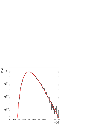
Figure 7: Probability distribution of the self-interaction potential (histogram) and a fit to a modified log Gaußian (continuous line).

This improved fit results in a better numerical estimate of the potential average,

$$\langle e^{-gTv[y]}\rangle_{y} = e^{-gTv_{0}}\,p_{1}\int_{0}^{\infty}dv\,e^{-gTv}\,e^{-\frac{1}{2p_{2}^{2}}(\ln(v)-p_{3})^{2}}$$ (59)

$$=: e^{-gTv_{0}}\,F_{(p_{i})}(gT),$$

which is of the same form as for the simplified fit in Eq. (49), but involves a more complex function $F_{(p_{i})}(x)$ defined by a parameter integral. The mass renormalization proceeds as above, $m_{\text{R}}^{2}=m^{2}+h^{2}/(8\pi^{2})\,v_{0}$, since $F_{(p_{i})}(gT)$ decays weaker than exponentially for large $T$, see App. D. Therefore, replacing $F_{(\alpha\beta)}(x)$ in Eq. (56) by $F_{(p_{i})}(x)$, we obtain our improved result for the effective action for the scalar photon.

At this point, it is important to stress that both fits do not only differ with respect to their quality of describing the data, but also with respect to their analytic properties. This becomes particularly apparent from the corresponding perturbative expansions. For instance, the simple fit leads to $F_{(\alpha\beta)}(gT)$, Eq. (50), which is completely analytic in $g$ and hence can be expanded in a well-converging Taylor series, as displayed in Eq. (104) in App. D. By contrast, the resulting auxiliary function $F_{(p_{i})}(gT)$ from the better fit gives rise to an asymptotic series upon expansion for $g\to 0^{+}$, as shown in Eq. (103).

Within the language of diagrammatic perturbation theory, the implications from the two fits are different. To see this, let us note that the ratio of successive loop contributions to a scalar photon proper vertex (obtained by expanding $\Gamma_{\text{QA}}[A]$ in terms of $A$) is proportional to the ratio of the corresponding expansion coefficients of the auxiliary function,

$$\frac{\Gamma_{\text{QA,R}}^{(n)}|_{l+1\,\,\text{loop}}}{\Gamma_{\text{QA,R}}^{(n)}|_{l\,\,\text{loop}}}\Bigg{|}_{\text{l.g. in}\,\,l}=-(l+n)\,\frac{F^{(l)}(gT=0)}{F^{(l-1)}(gT=0)}\,g,\quad\Gamma_{\text{QA,R}}^{(n)}=\frac{\delta^{n}\Gamma_{\text{QA,R}}[A=0]}{\delta A\dots\delta A},$$ (60)

where $F^{(l)}(gT=0)$ denotes the $l$th expansion coefficient of the corresponding auxiliary function (see, Eqs. (103) and (104)), and we have concentrated on the leading growth (l.g.) of the ratio for large $l$. The prefactor of $(l+n)$ arises from the propertime integration and can be traced back to the fact that the self-interaction potential $V$ is dimensionful in the scalar model. Now, for the two different fits, this coefficient ratio reads

$$\frac{\Gamma_{\text{QA,R}}^{(n)}|_{l+1\,\,\text{loop}}}{\Gamma_{\text{QA,R}}^{(n)}|_{l\,\,\text{loop}}}\Bigg{|}_{\text{l.g. in}\,\,l}=-g\,\times\left\{\begin{array}[]{ll}\frac{l+n}{\beta}&\text{for}\quad F_{(\alpha\beta)}\\ e^{p_{2}^{2}(l+1/2)-p_{3}}(1+\frac{n}{l})&\text{for}\quad F_{(p_{i})}\end{array}\right..$$ (61)

This implies that the proliferation of diagrams with increasing loop order translates to an increase of the expansion coefficient which is very different for the two fits. The simple fit, Eq. (46), leads to a mild increase of the expansion coefficients. Though the resulting perturbative series would not be convergent but asymptotic, the series would be immediately Borel summable. For instance, for the case of ScQED, it has recently been conjectured that the perturbation series even converges for the on-shell renormalized QED $n$-photon amplitudes in the quenched approximation [34].

For the better fit, Eq. (57), the coefficient ratio increases strongly, implying that a resummation requires generalized resummation techniques. Since the leading-growth behavior of the coefficients from the loop expansion are influenced by the combinatorics of diagrams, the conclusion for this perturbative combinatorics would be very different for the two fits. The lesson to be learned is that drawing a reliable conclusion about the analyticity structure of the perturbative expansion from the numerical estimate is very difficult. Different fits of similar quality can lead to very different analytic structures. However, since we have the fully resummed finite result numerically at our disposal, an analysis of the analytic structure may be viewed as a rather academic question. Notice also that the large $gT$ expansion is controlled by the small $v$ behavior, i.e., it is related to the approach to the “classical” region where $v\simeq v_{\rm min}$. This classical region corresponds to a subset of worldlines that are close to the minima of the action and thus resemble classical trajectories.

Let us finally point out one remarkable conclusion that can be drawn form the effective action (56). To one-loop order, the small-mass or large-photon-field limit of the effective action is of the form

$$\Gamma_{\text{1-loop}}[A]\big{|}_{\frac{hA}{m_{\text{R}}^{2}}\gg 1}\simeq-\frac{1}{64\pi^{2}}\int d^{4}x\,(hA)^{2}\ln\frac{hA}{m_{\text{R}}^{2}},$$ (62)

exhibiting a logarithmic increase, as is familiar from the Heisenberg-Euler QED effective action or the Coleman-Weinberg potential. This form implies that the massless $\phi$ field limit is not well defined for our scalar model; technically speaking, the $T$ integral is divergent at the upper bound in the massless limit. This becomes different, once the infinite number of diagrams of the quenched approximation is taken into account. These induce the $F_{(\dots)}(gT)$ function which vanishes for larger $T$, $F_{(\dots)}(gT\to\infty)\to 0$. This property renders the $T$ integrand finite even in the massless $\phi$ field limit. For instance, for the simple fit, the massless limit of $\Gamma_{\text{QA}}[A]$ can be evaluated analytically. Here, we just cite the result for the limit $A/h\ll 1$, for which the quenched approximation is expected to be more reliable,

$$\Gamma_{\text{QA,R}}[A]|_{m_{\text{R}}=0}=-\frac{[-\Gamma(-2-\alpha)]\cos\frac{\pi}{2}\alpha}{2^{5-3\alpha}\pi^{2(1-\alpha)}\beta^{\alpha}}\int d^{4}x\,(hA)^{2}\,\left(\frac{A}{h}\right)^{\alpha}[1+\mathcal{O}((A/h))].$$ (63)

The overall sign is, of course, still negative since $\alpha\simeq 0.79$. We conclude that a completely massless scalar model of the present type can be formulated consistently in the quenched approximation; it is only the perturbative expansion of this model that breaks down in the massless limit.

6 Conclusions and Outlook

The feasibility of a nonperturbative analysis in quantum field theory based on the worldline formalism has been demonstrated here. The approach combines the efficiency of worldline representations, i.e., having infinitely many Feynman diagrams in one worldline expression, with powerful numerical algorithms for the worldline integrals. As a major advantage of this approach, all continuous spacetime symmetries remain unaffected by numerical discretization procedures.

In the present exploratory study, we have considered a scalar model with cubic interaction in four dimensions in the quenched approximation which is the leading non-trivial order in a small-$N_{\text{f}}$ expansion. This approximation is expected to hold for small external field amplitudes but arbitrary values of the coupling. The model mimics scalar QED or Yukawa theory and is super-renormalizable though not finite. Therefore the divergence structure is rich enough to allow for a detailed study of the main difficulty of many field theoretic methods: understanding the origin and taming of divergencies. The combination of the propertime representation and the worldline discretization provides for a sufficient regularization, facilitating the identification of divergencies. Subsequently, the divergencies can be removed by fixing physical parameters by virtue of renormalization conditions on a nonperturbative level. It is particularly such a nonperturbative analysis of quantum field theories which sheds light on the fundamental problem whether a perturbative formulation gives an exactly correct account of divergencies [38]. For practical purposes, our divergence analysis may be helpful for technically similar problems, e.g., arising in many effective theories for polymer physics [39].

For the case of the effective action for soft scalar photons, we have performed this program explicitly. The result is a finite propertime parameter integral of Heisenberg-Euler type, containing all-order corrections in the coupling. These all-order contributions particularly modify the large-propertime behavior, in turn affecting the small-mass limit. We observe that the zero-mass limit surprisingly exists in the nonperturbative result, whereas perturbation theory is ill-defined in this limit. Hence, we conclude that the large logarithms for small masses from all quenched diagrams can be summed up to a finite result. Whether this feature persists beyond the quenched approximation remains an open issue.

At this point, a more detailed discussion of the interplay between the various parameters and approximation methods is in order. In the scalar model, we have three massive scales, implying two dimensionless parameters, e.g., $hA/m^{2}$ and $hA/h^{2}\equiv A/h$. In the limit $A/h\gg 1$, radiative scalar photon exchanges are suppressed and the perturbative loop expansion is expected to become reliable, almost independently of the value of $hA/m^{2}$; of course, for $hA/m^{2}\gg 1$, infinitely many couplings to the external field have to be taken into account. For $A/h\ll 1$, the systems is in the nonperturbative regime. In the additional limit of $hA/m^{2}\ll 1$, higher $\phi$ loops are suppressed by the mass threshold in comparison to radiative photon exchanges; hence, the quenched approximation is reliable in this limit. Whether this suppression of $\phi$ loops persists also in the massless limit of the scalar model is an open question. The fact that the massless limit exists in the quenched approximation may be taken as an indication for an affirmative answer. At least, there is no obvious reason for additional virtual $\phi$ loops to exhibit a problematic infrared behavior; on the contrary, virtual momenta flowing into the virtual loops rather serve as additional infrared regulators. In this sense, the quenched approximation with one virtual $\phi$ loop and soft zero-momentum external photons represents the case of highest sensitivity to the massless limit. To summarize, we expect the finiteness of the massless limit in the scalar model to persist beyond the quenched approximation; whether further $\phi$ loops give quantitatively sizable contributions to this result has to be checked by explicit computation. For this, the necessary inclusion of additional internal matter loops into our formalism appears to be feasible with our present technology. We would finally like to stress that the massless limit of the scalar model may be a peculiarity induced by the existence of a massive coupling, and it might not translate to a similar property of renormalizable models such as QED or Yukawa interactions. For instance in spinor QED, an interacting massless limit of the soft-photon action is inhibited either by triviality or by chiral symmetry breaking [35].

From a technical perspective, we have developed further the algorithmic tools of worldline numerics. Beyond those techniques that so far have successfully been applied to perturbative computations, the use of probability distributions renders the algorithms extremely efficient. For instance, the effective action, i.e., the generating functional of infinitely many soft photon amplitudes, has been derived from one single distribution (of the self-interaction potential). A further illustrative example for the harmonic oscillator is given in App. C. We are convinced that the method will find a variety of applications, given the large number of problems that are being tackled by propertime methods.

Our work paves the way for many generalizations: for instance, both the worldline formalism as well as our worldline numerics are well suited for a study of propagators in coordinate space, where the scale set by the propagation distance represents one further technical challenge. The study of propagators appears mandatory for an analysis of renormalizable theories such as (scalar) QED in $D=4$. In these cases, our simplified mass renormalization will no longer be sufficient and the renormalized mass needs to be fixed with the aid of the propagator’s correlation length.

Moreover, a generalization to gauge interactions will require a more careful treatment as far as the discretization is concerned. Our present method if applied to a gauge theory with a charged $\phi$ field would not satisfy current conservation which is essential for maintaining gauge invariance. More refined algorithms are required and are a subject of current development.

Appendix A Derivation of the effective action

Here, we derive the worldline representation of the Schwinger functional and the effective action for the scalar photon field $\Gamma[A]$, Eq. (9). We start by citing the Schwinger functional as given in Eq. (2) with the insertion of the worldline form of $S_{\text{eff}}$ of Eq. (3),

$$Z[J]\equiv e^{W[J]}=\int\mathcal{D}\hat{A}\,\exp\left[-\int_{x}\frac{1}{2}(\partial_{\mu}\hat{A})^{2}+\int_{T}\Big{\langle}e^{\int_{x}j\hat{A}}\Big{\rangle}_{x}+\int_{x}J\hat{A}\right],$$ (64)

where we have used the worldline current representation of Eq. (7), and introduced the abbreviation

$$\int_{T}:=\frac{1}{2(4\pi)^{D/2}}\int_{0}^{T}\frac{dT}{T^{1+D/2}}\,e^{-m^{2}T}.$$ (65)

Let us first expand the worldline exponential, such that the $\hat{A}$ integral becomes Gaußian at each order of the Taylor sum,

$$Z[J] = \sum_{0}^{\infty}\frac{1}{n!}\int_{T_{1}}\dots\int_{T_{n}}\left\langle\int\mathcal{D}\hat{A}\,e^{-\int_{x}\frac{1}{2}(\partial\hat{A})^{2}}e^{\int_{x}\hat{A}(j_{1}+\dots+j_{n}+J)}\right\rangle_{x_{1}\dots x_{n}}$$ (66)

$$= \sum_{0}^{\infty}\frac{1}{n!}\int_{T_{1}}\dots\int_{T_{n}}\left\langle e^{\frac{1}{2}\int_{x}K_{n}^{J}\Delta K_{n}^{J}}\right\rangle_{x_{1}\dots x_{n}}$$

$$\equiv e^{W[J]},$$

where we have introduced the generating functional of connected Green’s functions $W[J]$ in the last line, and have defined the sum of currents

$$K_{n}^{J}=J+\sum_{i}^{n}j_{i}.$$ (67)

The kernel $\Delta$ denotes again the scalar photon propagator as given in Eq. (10). Note that Eq. (66) is an exact representation of the Schwinger functional without any approximation so far. The classical field $A$ (conjugate to the source $J$) is obtained from $W[J]$ by functional differentiation (cf. Eq. (6)),

$$A = \frac{\delta W[J]}{\delta J}$$ (68)

$$= \Delta\,J+e^{-W[J]}\sum_{n}\frac{1}{n!}\int_{T_{1}\dots T_{n}}\left\langle\Delta\sum_{i=1}^{n}j_{i}\,\,e^{\frac{1}{2}\int_{x}K_{n}^{J}\Delta K_{n}^{J}}\right\rangle_{x_{1}\dots x_{n}}.$$

A partial inversion of this equation gives,

$$J=\Delta^{-1}\,A-e^{-W}\sum_{n}\frac{1}{n!}\,\int_{T_{1}\dots T_{n}}\left\langle\sum_{i=1}^{n}j_{i}\,\,e^{\frac{1}{2}\int_{x}K_{n}^{J}\Delta K_{n}^{J}}\right\rangle_{x_{1}\dots x_{n}},$$ (69)

with $\Delta^{-1}=-\partial^{2}$. Note that this is an implicit definition of $J=J[A]$, since $K_{n}^{J}$ in the exponent on the right-hand side still depends on $J$. Nevertheless, these definitions can be used to give an implicit definition of the exact effective action for the scalar photons $\Gamma[A]$ (cf. Eq. (5)),

$$\Gamma[A]=-W[J[A]]+\int_{x}A\,J[A].$$ (70)

Explicit representations can be found in the quenched approximation that consists of dropping all terms involving worldline correlators of different worldline currents, $\langle j_{i}\dots j_{j}\rangle_{x_{i}\dots x_{j}}\to 0$, $i\neq j$. In this approximation, the Schwinger functional Eq. (66) can be written as

$$e^{W_{\text{QA}}[J]} = e^{\frac{1}{2}\int_{x}J\Delta J}\sum_{n}\frac{1}{n!}\int_{T_{1}}\Big{\langle}e^{\frac{1}{2}\int_{x}j_{1}\Delta j_{1}+\int_{x}J\Delta j_{1}}\Big{\rangle}_{x_{1}}\dots\int_{T_{n}}\Big{\langle}e^{\frac{1}{2}\int_{x}j_{n}\Delta j_{n}+\int_{x}J\Delta j_{n}}\Big{\rangle}_{x_{n}}$$ (71)

$$= \exp\left[\frac{1}{2}\int_{x}J\Delta J+\int_{T}\Big{\langle}e^{\frac{1}{2}\int_{x}j\Delta j+\int_{x}J\Delta j}\Big{\rangle}_{x}\right].$$

The corresponding representation of the classical field in quenched approximation boils down to

$$A=\Delta\,J+\int_{T}\Big{\langle}e^{\frac{1}{2}\int_{x}j\Delta j+\int_{x}J\Delta j}\,\Delta\,j\Big{\rangle}_{x}.$$ (72)

Note that, even in the quenched approximation, this equation cannot be inverted explicitly for the current,

$$J=\Delta^{-1}A-\int_{T}\Big{\langle}e^{\frac{1}{2}\int_{x}j\Delta j+\int_{x}J\Delta j}\,j\Big{\rangle}_{x}.$$ (73)

We take this equation as the implicit definition of $J=J[A]$. By virtue of Eq. (70), this allows to express the effective action $\Gamma_{\text{QA}}[A]$ intermediately in terms of $J[A]$,

$$\Gamma_{\text{QA}}[A]=\frac{1}{2}\int_{x}J\Delta J+\int_{T}\Big{\langle}e^{\frac{1}{2}\int_{x}j\Delta j+\int_{x}J\Delta j}\,(J\Delta j-1)\Big{\rangle}_{x}.$$ (74)

Now, $J[A]$ of Eq. (73) can be iteratively inserted into Eq. (74). As a consequence, the iteration terminates after the first order by means of the quenched approximation, since the higher orders involve multi-worldline current correlators. The result can be displayed in closed form,

$$\Gamma_{\text{QA}}[A]=\int_{x}\frac{1}{2}(\partial_{\mu}A)^{2}-\frac{1}{2(4\pi)^{D/2}}\int_{0}^{\infty}\frac{dT}{T^{1+D/2}}\Big{\langle}e^{\frac{1}{2}\int_{x}j\Delta j+\int_{x}jA}\Big{\rangle}_{x},$$ (75)

which serves as the starting point of our investigation in Eq. (9).

Appendix B Worldline generation: “d loops”

Here we describe a new algorithm for generating open or closed worldlines ab initio, which is used for most numerical studies in the present work. The algorithm generates worldlines by a suitable doubling of points, starting from a small number (e.g., from 1 point); hence we call the resulting worldlines “d loops” (closed) or “d lines” (open). The algorithm is reminiscent of a heat-bath algorithm, as was used in earlier worldline numerical studies [19], but does not require dummy thermalization sweeps.

Let us first consider closed “d loops”. By appropriate rescaling, the Gaußian velocity distribution can always be brought to unit loop form,

$$P[y]=e^{-\frac{1}{4}\int_{0}^{1}\,dt\,\left(\frac{dy(t)}{dt}\right)^{2}}.$$ (76)

Discretizing the $t$ derivative by an asymmetric nearest-neighbor form, $dy/dt=(y_{i}-y_{i-1})/\Delta t$, with $i=1,\dots,N_{0}$, the distribution becomes

$$P_{N_{0}}[y]\to e^{-\frac{N_{0}}{4}\sum_{i=1}^{N_{0}}\,(y_{i}-y_{i-1})^{2}}.$$ (77)

The probability for the location of the $i$’th point is

$$p_{y_{i}}=e^{-\frac{N_{0}}{4}[2y_{i}^{2}-2y_{i}(y_{i+1}+y_{i-1})]\dots}=e^{-\frac{N_{0}}{4}\,2[y_{i}-\frac{1}{2}(y_{i+1}+y_{i-1})]^{2}\dots},$$ (78)

such that $y_{i}$ is in a Gaußian heat bath of the algebraic mean of its nearest neighbors. The crucial point now is that we can add another $N_{0}$ points $y_{i^{\prime}}$ in between with the following probability distribution,

$$p_{y_{i^{\prime}},y_{i^{\prime}+1}}=e^{-\frac{2N_{0}}{4}[2(y_{i^{\prime}}-\frac{1}{2}(y_{i}+y_{i-1}))^{2}+2(y_{i^{\prime}+1}-\frac{1}{2}(y_{i+1}+y_{i}))^{2}]\dots},$$ (79)

such that the new total probability distribution for $y_{i}$ becomes

$$p_{y_{i}}\to p_{y_{i}}p_{y_{i^{\prime}},y_{i^{\prime}+1}}=e^{-\frac{2N_{0}}{4}\,2\,[y_{i}-\frac{1}{2}(y_{i^{\prime}+1}+y_{i^{\prime}})]^{2}\dots}.$$ (80)

Note that the probability distribution for the doubled points $y_{i^{\prime}}$ in Eq. (79) has been adjusted such that the probability distribution for the point $y_{i}$ has lost its dependence on $y_{i+1}$ and $y_{i-1}$; $y_{i}$ only feels the heat bath of the new points $y_{i^{\prime}}$ and $y_{i^{\prime}+1}$. Correspondingly, the full distribution for the $N_{0}+N_{0}=2N_{0}=N_{1}$ points reads:

$$P_{N_{1}}[y]\to e^{-\frac{N_{1}}{4}\sum_{i=1}^{N_{1}}\,(y_{i}-y_{i-1})^{2}},$$ (81)

where we have redefined $y_{i}\to y_{2i}$, $y_{i^{\prime}}\to y_{2i-1}$.

Now the recipe for the “d loop” algorithm generating closed worldlines with $N$ ppl is obvious:

• Begin with one arbitrary point $N_{0}=1$, $y_{N}$.

• Create an $N_{1}=2$ loop, i.e., add a point $y_{N/2}$ that is distributed in the heat bath of $y_{N}$ with

  $$e^{-\frac{N_{1}}{4}2(y_{N/2}-y_{N})^{2}}.$$ (82)

• Iterate this procedure, creating an $N_{k}=2^{k}$ppl loop by adding $2^{k-1}$ points $y_{{qN}/{N_{k}}}$, $q=1,3,\dots,N_{k}-1$ with distribution

  $$e^{-\frac{N_{k}}{4}2[y_{qN/N_{k}}-\frac{1}{2}(y_{(q+1)N/N_{k}}+y_{(q-1)N/N_{k}})]^{2}}.$$ (83)

• Terminate the procedure if $N_{k}$ has reached $N_{k}=N$ for unit loops with $N$ ppl.

• For an ensemble with common center of mass, shift each whole loop accordingly.

Open worldlines (“d lines”) can be generated analogously by starting with the end points $x_{\text{I}}=y_{0}$ and $x_{\text{F}}=y_{N+1}$ and filling $N$ new points in between by the same doubling procedure.

In comparison with existing worldline generator algorithms such as the “f loop” and “v loop” algorithms of [22], all algorithms share the property that each generated random number is used for a worldline; in particular, no dummy thermalization sweeps are necessary. Similarly to the “f loop” algorithm, “d loops” produce worldlines with $N=2^{l}$ ppl, $l\in\mathbbm{N}$, whereas the “v loop” algorithm can produce any $N\in\mathbbm{N}$. “f loops” by Fourier transformation discretize the derivative $\dot{x}$ implicitly such that the operator $d^{2}/d\tau^{2}$ is diagonal in Fourier space, whereas “v loops” and “d loops” use the asymmetric nearest-neighbor discretization $\dot{x}\sim x_{i}-x_{i-1}$. The later has proved to approach the continuum limit in problems with scalar interactions faster than the Fourier decomposition [22]. In comparison to “v loops”, the present “d loop” algorithm requires less algebraic operations and hence is faster by some ten percent.

Appendix C Harmonic oscillator

As an instructive example of the use of the Monte-Carlo method involving distribution fits, let us study the harmonic oscillator. The propagator for a harmonic oscillator can be written in the form

$$G(T,R)=\int_{x(0)=x_{\text{I}}}^{x(T)=x_{\text{F}}}{\cal D}x\exp\{-\frac{1}{2}\;\int_{0}^{T}d\tau\;\dot{x}^{2}+\omega^{2}x^{2}\},\quad R=|x_{\text{F}}-x_{\text{I}}|.$$ (84)

In the language of quantum field theory, this corresponds to the heat kernel of a $D=1$ dimensional scalar field theory, coupling to a constant “potential” $\omega^{2}$. In the notation of worldline ensemble averages, this propagator can be written as

$$G(T,R)=\left\langle\exp\left[-\frac{1}{2}\int_{0}^{T}d\tau\,\omega^{2}x^{2}\right]\right\rangle_{x_{\text{I}}}^{x_{\text{F}}}.$$ (85)

Introducing the $T$ scaling as outlined in Eq.(21) yields

$$G(T,R)=\Big{\langle}\exp\left[-\frac{1}{2}\omega^{2}T^{2}\int_{0}^{1}dt\;y^{2}\right]\Big{\rangle}_{\sqrt{T}y_{\text{I}}}^{\sqrt{T}y_{\text{F}}}.$$ (86)

The integral is Gaußian and can be done analytically [36]. For $x_{\text{I}}=x_{\text{F}}=0$, it is simply given by

$$G(T,R=0)=\sqrt{\frac{\omega T}{\sinh\omega T}}.$$ (87)

In Fig. 8, we plot the result of our Monte-Carlo calculation with $N=2^{14}$ ppl for $\omega=1$.

The agreement with the analytical result is excellent, coinciding for more than 10 orders of magnitude with a very small error.

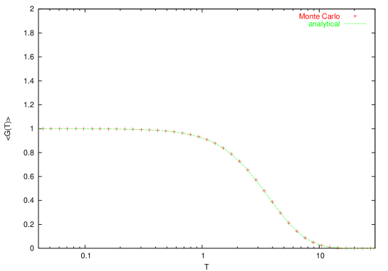
Figure 8: Propagator for the harmonic oscillator for $x_{\text{I}}=x_{\text{F}}=0$, for $N=2^{14}$ ppl and $\omega=1$ and 10⁴ worldline ensembles. The Monte-Carlo calculation (points) is shown in comparison to the analytical calculation of Eq. (87) (line).

However, the Monte-Carlo calculation is not free from problems, as becomes visible, e.g., for the ground state energy. The latter can be calculated from the standard identity

$$E_{0}=\lim_{T\rightarrow\infty}-\frac{\log(G(T))}{T}.$$ (88)

In Fig. 9, we plot $-\log(G(T))/T$ versus $T$ for large values of $T$, comparing the analytical result to the Monte-Carlo calculation with $n_{\text{L}}=10^{4}$ and $10^{6}$ worldline ensembles. As is obvious from the figure, the Monte-Carlo approaches the analytical result for intermediate $T$, but ultimately departs from the analytical result from some larger value of $T$ on. This point depends on the statistics of the Monte-Carlo. This phenomena is well known in the literature and is usually referred to as the “classical collapse” [37].

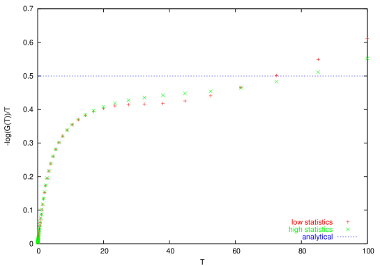
Figure 9: $-\log G(T)/T$ for the harmonic oscillator. Shown is the exact analytical result for $\omega=1$ (dashed line) and the Monte-Carlo results with $2^{10}$ ppl for $10^{4}$ and $10^{6}$ worldline ensembles.

We can cast the problem into our language by introducing the distribution of potentials, i.e.,

$$G(T,R=0)=\int dv_{2}P(v_{2})\exp\left[-\frac{1}{2}\omega^{2}T^{2}v_{2}\right],$$ (89)

where the self-interaction potential is a local expression here:

$$v_{2}=\int_{0}^{1}dt\;y^{2}.$$ (90)

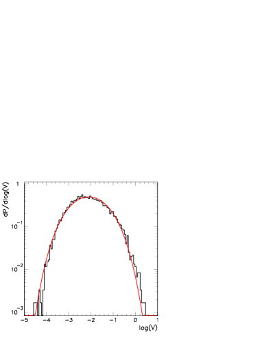
Figure 10: Potential distribution $P(v_{2})$ for the harmonic oscillator for $N=2^{10}$ ppl and 10⁶ worldline ensembles. Also shown is the fit to the proposed distribution.

From Eq. (89), we observe that the limit $T\rightarrow\infty$ is controlled by $v_{2}\rightarrow 0$. However, the distribution of potentials $P(v_{2})$ in this small $v_{2}$ limit is poorly determined, owing to the lack of statistics, $P(v_{2})\rightarrow 0$. A typical distribution $P(v_{2})$ is displayed in Fig. 10 for $N=2^{14}$ ppl. For any fixed number of worldline ensembles, there is always a minimum value of the potential, $v_{2\,{\rm min}}$, such that for any $T$ larger than that determined by

$$\frac{1}{2}\omega^{2}T^{2}v_{2{\rm min}}\sim 1,$$ (91)

the potential distribution $P(v_{2})$ is not well represented by the given statistical ensemble. This can be observed in Fig. 9, where an increase of the size of the ensemble enlarges the region in $T$ for which the Monte-Carlo calculation is valid.

Our alternative method circumvents this problem by using an analytical parameterization of $P(v_{2})$ which has an appropriate behavior for low $v_{2}$. For instance, the normalized trial function

$$P(v_{2})=\hat{\mathcal{N}}\,e^{-(a/v_{2}+bv_{2})},\quad\hat{\mathcal{N}}^{-1}=2\sqrt{\frac{a}{b}}\,K_{1}(2\sqrt{ab}),$$ (92)

gives a reasonably good description of $P(v_{2})$ and reproduces the large $T$ behavior. Here $a\simeq 0.11$ and $b\simeq 18.4$ are constants determined by a fit to the potential distribution.

From Eq. (89), we immediately get a numerical estimate for the propagator,

$$G(T,R=0)\big{|}_{P(v_{2})}=\sqrt{\frac{2b}{2b+\omega^{2}T^{2}}}\,\frac{K_{1}(2\sqrt{ab+a\omega^{2}T^{2}/2})}{K_{1}(2\sqrt{ab})},$$ (93)

such that the large $T$ limit gives the ground state energy,

$$E_{0}\big{|}_{P(v_{2})}=\sqrt{2a}\,\omega,$$ (94)

which is in good agreement with the exact answer.

Appendix D Analysis of the potential fit function

Here we analyze some properties of the auxiliary function $F_{(p_{i})}(x)$ introduced in Eq. (59) which are relevant for the mass renormalization as well as the weak- and strong-coupling behavior of the effective action for the scalar photon in Sect. 5. This function is defined by

$$F_{(p_{i})}(x)=p_{1}\int_{0}^{\infty}dv\,e^{-xv}\,e^{-\frac{1}{2p_{2}^{2}}(\ln(v)-p_{3})^{2}},$$ (95)

with the $p_{i}$ being constant fit parameters and $x\equiv gT$ as in the main text. We observe that the exponent becomes large (but negative) for small as well as large $v$ with an extremum in between. This suggest to evaluate the integral approximately by steepest descent in order to obtain analytic information about its behavior, e.g., for larger propertimes $T$. To be precise, we perform the approximation to the following order,

$$F_{(p_{i})}(x) = p_{1}\int_{0}^{\infty}dv\,e^{-f(v)}$$ (96)

$$\simeq p_{1}e^{-f(v_{\text{E}})}\int_{0}^{\infty}dv\ e^{-\frac{1}{2}(v-v_{\text{E}})^{2}\,f^{\prime\prime}(v_{\text{E}})+\dots},$$

where

$$f(v)=x\,v+\frac{1}{2p_{2}^{2}}[\ln(v)-p_{3}]^{2},$$ (97)

such that the extremum $v_{\text{E}}$ which is a minimum of $f(v)$ is determined by $0=f^{\prime}(v_{\text{E}})$; the latter leads to a transcendental equation

$$xv_{\text{E}}=\frac{p_{3}-\ln(v_{\text{E}})}{p_{2}^{2}},$$ (98)

that can be brought to a standard form,

$$p_{2}^{2}\,e^{p_{3}}\,x=w\,e^{w},\quad\text{with}\quad w=p_{3}-\ln v_{\text{E}}.$$ (99)

This form, $z=w\,e^{w}$, is the defining equation of the “product logarithm” $w(z)$ by which we can express the extremum of the integrand as a function of $x$:

$$v_{\text{E}}(x)=\frac{1}{p_{2}^{2}}\,\frac{w(p_{2}^{2}e^{p_{3}}\,x)}{x}.$$ (100)

One important property of the product logarithm is its asymptotic behavior for large argument, $w(z)\to\ln z$ for $z\to\infty$, such that the extremum goes to zero for large propertimes $x=gT$. By contrast, the “inverse width” of the fluctuations around the extremum diverges for large propertimes and vanishing extremum,

$$f^{\prime\prime}(v_{\text{E}})=\frac{1}{p_{2}^{2}}\,\frac{1+p_{3}-\ln v_{\text{E}}}{v_{\text{E}}^{2}},$$ (101)

such that the steepest-descent approximation is expected to be accurate in this limit. Putting it all together, the steepest-descent approximation of Eq. (95) becomes upon insertion of Eqs. (97), (100) and (101) into Eq. (96),

$$F_{(p_{i})}(gT\gg 1) \simeq \sqrt{\frac{\pi}{2}}\frac{p_{1}}{p_{2}}(p_{2}^{2}e^{p_{3}})^{-1/p_{2}^{2}}\,\frac{\ln^{1/2}gT}{(gT)^{1+(1/p_{2}^{2})}}\,$$ (102)

$$\times\exp\left\{-\frac{1}{p_{2}^{2}}\left[\ln\left(\frac{1}{p_{2}^{2}}\frac{\ln(p_{2}^{2}e^{p_{3}}gT)}{gT}\right)-p_{3}\right]^{2}\right\}.$$

Here we have already inserted the asymptotic form of the product logarithm for large argument. In this large-$gT$ limit, the term $\sim\exp(-(1/p_{2}^{2})\ln^{2}gT)$ dominats the decay of $F_{(p_{i})}(gT)$, which is weaker than exponential but stronger than power-like. As a consequence, $F_{(p_{i})}(gT)$ does not contribute any finite part to the mass renormalization, due to the prescription specified in Eq. (54), but guarantees the finiteness of the effective action $\Gamma_{\text{QA}}[A]$ in the massless-$\phi$ limit.

Let us now study the opposite limit of small $x=gT$ corresponding to a perturbative expansion. For this, the first exponential in the definition of $F_{(p_{i})}(gT)$ in Eq. (95) can be expanded and the $v$ integral can be done order by order to give

$$F_{(p_{i})}(gT)=\sqrt{2\pi}\,p_{1}p_{2}\,\sum_{m=0}^{\infty}\,\frac{e^{\frac{1}{2}(m+1)[(m+1)p_{2}^{2}+2p_{3}]}}{m!}\,(-gT)^{m}.$$ (103)

The $m$th order in this expansion corresponds to the $l=m+1$-loop order in perturbation theory. For large $m$, the leading growth of the expansion coefficient is $\sim\exp(m^{2}/2-m\ln m)$ by use of Stirling’s formula. Hence, this perturbative expansion gives an asymptotic series in the coupling.

For comparison, we mention the analogous expansion for the simple-fit result,

$$F_{(\alpha\beta)}(gT)=\sum_{m=0}^{\infty}\frac{1}{\beta^{m}}\,\frac{\Gamma(m+\alpha+1)}{\Gamma(m+1)\Gamma(\alpha+1)}\,(-gT)^{m},$$ (104)

implying a weaker leading growth of the expansion coefficient $\sim m^{\alpha}$. This series is absolutely convergent for $|gT/\beta|<1$.

References

-
[1]
W. Heisenberg and H. Euler,
Z. Phys. 98, 714 (1936);
V. Weisskopf, K. Dan. Vidensk. Selsk. Mat. Fys. Medd. 14, 1 (1936). - [2] S. R. Coleman and E. Weinberg, Phys. Rev. D 7, 1888 (1973).
- [3] R.P. Feynman, Phys. Rev. 80, 440 (1950); 84, 108 (1951).
-
[4]
M. B. Halpern and W. Siegel,
Phys. Rev. D 16, 2486 (1977);
M. B. Halpern, A. Jevicki and P. Senjanovic, Phys. Rev. D 16, 2476 (1977);
A. M. Polyakov, “Gauge Fields And Strings,” Harwood, Chur (1987). - [5] Z. Bern and D.A. Kosower, Nucl. Phys. B362, 389 (1991); B379, 451 (1992).
- [6] M.J. Strassler, Nucl. Phys. B385, 145 (1992).
-
[7]
M. G. Schmidt and C. Schubert,
Phys. Lett. B318, 438 (1993)
[hep-th/9309055];
M. Reuter, M. G. Schmidt and C. Schubert, Annals Phys. 259, 313 (1997) [arXiv:hep-th/9610191];
R. Shaisultanov, Phys. Lett. B 378, 354 (1996) [arXiv:hep-th/9512142]. - [8] For a review, see C. Schubert, Phys. Rept. 355, 73 (2001) [arXiv:hep-th/0101036].
- [9] Z. Bern, D.C. Dunbar, T. Shimada, Phys. Lett. B 312 (1993) 277, hep-th/9307001.
- [10] D.C. Dunbar, P.S. Norridge, Nucl. Phys. B 433 (1995) 181, hep-th/9408014.
- [11] D. Cangemi, E. D’Hoker, G. Dunne, Phys. Rev. D 51 (1995) 2513, hep-th/9409113.
- [12] F. A. Dilkes and D. G. C. McKeon, Phys. Rev. D 53, 4388 (1996) [arXiv:hep-th/9509005].
- [13] S.L. Adler, C. Schubert, Phys. Rev. Lett. 77 (1996) 1695, hep-th/9605035.
- [14] V.P. Gusynin, I.A. Shovkovy, Can. J. Phys. 74 (1996) 282, hep-ph/9509383; J. Math. Phys. 40 (1999) 5406, hep-th/9804143.
- [15] C. D. Fosco, J. Sánchez-Guillén and R. A. Vázquez, Phys. Rev. D 69, 105022 (2004) [arXiv:hep-th/0310191].
- [16] F. Bastianelli and C. Schubert, JHEP 0502, 069 (2005) [arXiv:gr-qc/0412095].
- [17] L. Magnea, R. Russo, and S. Sciuto, CERN-PH-TH/2004-244, hep-th/0412087.
- [18] F. Brummer, M. G. Schmidt and Z. Tavartkiladze, arXiv:hep-th/0412284.
- [19] H. Gies and K. Langfeld, Nucl. Phys. B 613, 353 (2001) [arXiv:hep-ph/0102185]; Int. J. Mod. Phys. A 17, 966 (2002) [arXiv:hep-ph/0112198].
- [20] M. G. Schmidt and I. O. Stamatescu, Nucl. Phys. Proc. Suppl. 119, 1030 (2003) [arXiv:hep-lat/0209120]; Mod. Phys. Lett. A 18, 1499 (2003).
- [21] K. Langfeld, L. Moyaerts and H. Gies, Nucl. Phys. B 646, 158 (2002) [arXiv:hep-th/0205304].
- [22] H. Gies, K. Langfeld and L. Moyaerts, JHEP 0306, 018 (2003) [arXiv:hep-th/0303264]; arXiv:hep-th/0311168.
-
[23]
G.C. Wick, Phys. Rev. 96, 1124 (1954);
R.E. Cutkosky, Phys. Rev. 96, 1135 (1954). - [24] I. K. Affleck, O. Alvarez and N. S. Manton, Nucl. Phys. B 197, 509 (1982).
-
[25]
R. Rosenfelder and A. W. Schreiber,
Phys. Rev. D 53, 3337 (1996)
[arXiv:nucl-th/9504002];
C. Alexandrou, R. Rosenfelder and A. W. Schreiber, Phys. Rev. A 59, 1762 (1999) [arXiv:hep-th/9809101]; C. Alexandrou, R. Rosenfelder and A. W. Schreiber, Phys. Rev. D 62, 085009 (2000) [arXiv:hep-th/0003253]. - [26] J. Sánchez-Guillén and R. A. Vázquez, Phys. Rev. D 65, 105001 (2002) [arXiv:hep-th/0201065].
- [27] C. Savkli, J. Tjon and F. Gross, Phys. Rev. C 60, 055210 (1999) [Erratum-ibid. C 61, 069901 (2000)] [arXiv:hep-ph/9906211]; arXiv:nucl-th/0404068.
- [28] N. Brambilla and A. Vairo, Phys. Rev. D 56, 1445 (1997) [arXiv:hep-ph/9703378].
- [29] L. Alvarez-Gaume, Commum. Math. Phys. 90, 161, (1983).
- [30] C. Fosco, [arXiv:hep-th/0404068].
- [31] C. M. Bender, K. A. Milton and V. M. Savage, Phys. Rev. D 62, 085001 (2000) [arXiv:hep-th/9907045].
- [32] H. Gies and J. Hämmerling, [arXiv:hep-th/0505072].
- [33] C. Fosco, J.S. Sánchez-Guillén, and R.A. Vázquez, in preparation (2005).
- [34] G. V. Dunne and C. Schubert, [arXiv:hep-th/0409021].
-
[35]
M. Gockeler, R. Horsley, V. Linke, P. Rakow, G. Schierholz and H. Stuben,
Phys. Rev. Lett. 80, 4119 (1998)
[arXiv:hep-th/9712244];
H. Gies and J. Jaeckel, Phys. Rev. Lett. 93, 110405 (2004) [arXiv:hep-ph/0405183]. - [36] C. Itzykson and J.B. Zuber, Quantum field theory, Mc Graw Hill, 1980, New York.
- [37] S.K. Kauffmann and J. Rafelski, Z. Phys. C 24, 157 (1984).
- [38] J. Glimm and A.M. Jaffe, Quantum Physics. A functional integral point of view, New York, Springer (1981).
- [39] F. David, K. Wiese, [arXiv:cond-mat/0409765].