Solving Bethe-Salpeter equation in Minkowski space

Abstract

We develop a new method of solving Bethe-Salpeter (BS) equation in Minkowski space. It is based on projecting the BS equation on the light-front (LF) plane and on the Nakanishi integral representation of the BS amplitude. This method is valid for any kernel given by the irreducible Feynman graphs. For massless ladder exchange, our approach reproduces analytically the Wick-Cutkosky equation. For massive ladder exchange, the numerical results coincide with the ones obtained by Wick rotation.

1 Introduction

BS equation SB_PR84_51 is an important tool to study the relativistic bound state problem in a field theory framework (see for review nakanishi ). For a bound state of total momentum $p$ and in case of equal mass particles, it reads

$$\Phi(k,p) = \frac{i^{2}}{\left[(\frac{p}{2}+k)^{2}-m^{2}+i\epsilon\right]\left[(\frac{p}{2}-k)^{2}-m^{2}+i\epsilon\right]}$$ (1)

$$\times \int\frac{d^{4}k^{\prime}}{(2\pi)^{4}}iK(k,k^{\prime},p)\Phi(k^{\prime},p),$$

where $\Phi$ is the BS amplitude, $iK$ the interaction kernel, $m$ the mass of the constituents and $k$ their relative momentum. We will denote by $M=\sqrt{p^{2}}$ the total mass of the bound state, and by $B=2m-M$ its binding energy.

It was recognized from the very beginning that, when formulated in Minkowski space, the BS equation has singularities which make difficult to find its solution. These singularities are due to the free propagators of the constituent particles

$$G_{0}^{(12)}(k,p)=G_{0}^{(1)}G_{0}^{(2)}=$$

$$=\frac{i}{(\frac{p}{2}+k)^{2}-m^{2}+i\epsilon}\;\frac{i}{(\frac{p}{2}-k)^{2}-m^{2}+i\epsilon}$$ (2)

but can also result from the interaction kernel itself.

To overcome this difficulty, Wick WICK_54 formulated the BS equation in the Euclidean space, by rotating the relative energy in the complex plane $k_{0}\to ik_{0}$. This ”Wick rotation” led to a well defined integral equation which can be solved by standard methods. Most of practical applications of the BS equation have been achieved using this technique nakanishi and recent developments make its solution a trivial numerical task NT_FBS_96 . Another method – the variational approach in the configuration Euclidean space – was recently developed in efimov . Whereas the total mass of the system is unchanged by the Wick rotation, the original BS amplitude is however lost and the ”rotated” one can no longer be used in calculating other physical observables, like for instance form factors.

Thus, fifty years after its formulation, obtaining the BS solutions in the Minkowski space is still a field of active research. A successful attempt was presented in KW , based on the Nakanishi integral representation of the BS function nak63 . However, formal developments displayed in KW are a matter of art and the obtained equation has been derived and solved only for the ladder kernel. Another approach in Minkowski space for separable interactions was developed in bbmst and applied to the nucleon-nucleon system. On another hand, an equation obtained by projecting the original BS equation on the LF plane, was derived and solved in sfcs . An approximate LF kernel was there obtained as an expansion of the BS one but the original BS amplitude has not been reconstructed from its LF projection.

The aim of this paper and the forthcoming one is to present a new method of solving the BS equation without using the Wick rotation. Our method is based on an integral transform of the initial equation which removes the singularities of the BS amplitude. This integral transform consists in projecting the BS equation on the LF plane, defined by $\omega\cdot x=0$ with $\omega^{2}=0$ cdkm . The particular choice $\omega=(\omega_{0},\vec{\omega})=(1,0,0,-1)$ results in the standard LF form $t+z=0$ and in the LF projection used in sfcs . In our approach, the BS amplitude maps onto the LF wave function while the transformed equation – in contrast to sfcs – is derived without any approximation. This equation remains equivalent to the original BS one, therefore providing the same binding energies, and the initial BS amplitude is easily reconstructed from its solution. Although results presented here concern only the ladder kernel, our method is not restricted to a particular interaction. For more complicated kernels, e.g. the cross box, calculations become more lengthy, but the additional difficulties are due to evaluating the Feynman diagram itself and not to the solution of the equation.

In order to present the method more distinctly, we consider the case of zero total angular momentum and spinless particles.

The plan of the paper is the following. In sect. 2, we give the integral transform used to project the BS equation on the LF plane and we derive a new and equivalent equation. In sect. 3, the corresponding ladder exchange kernel is calculated analytically. In sect. 4, the numerical solutions for the ladder case are found and compared to the results obtained using other methods in Euclidean space. Sect. 5 contains concluding remarks. Details of the calculations are given in appendices A, B and C. The results concerning cross box kernels are presented in the next paper ckII .

2 Projecting the BS equation on the LF plane

Our method is inspired by an existing relation between the BS amplitude $\Phi(k,p)$ and the two-body LF wave function $\psi(\vec{k}_{\perp},x)$. This wave function can be obtained by projecting the BS amplitude on the LF plane. We will apply below the LF projection to the BS equation in Minkowski space. Though this projection can be considered as a formal transform, we will start by reviewing its derivation, in order to show more clearly how the singular behaviour of $\Phi(k,p)$ gives rise to a non-singular $\psi(\vec{k}_{\perp},x)$.

BS amplitude is defined as the matrix element between the vacuum $\langle 0|$ and a state $|p\rangle$ of the time ordered product of two Heisenberg operators:

$$\Phi(x_{1},x_{2},p)=\langle 0|T\left\{\varphi(x_{1})\varphi(x_{2})\right\}|p\rangle.$$ (3)

In general, the state vector $|p\rangle$ can be taken in different representations. In the LF quantization, it has the form: (see e.g. eq. (3.1) from cdkm ):

$$|p\rangle = \int\;\psi(k_{1},k_{2},p,\omega\tau)2(\omega\cdot p)\delta(k_{1}+k_{2}-p-\omega\tau)d\tau$$ (4)

$$\times (2\pi)^{3/2}\;\frac{d^{3}k_{1}}{(2\pi)^{3/2}\sqrt{2\varepsilon_{k_{1}}}}\frac{d^{3}k_{2}}{(2\pi)^{3/2}\sqrt{2\varepsilon_{k_{2}}}}\;a^{\dagger}_{\vec{k}_{1}}a^{\dagger}_{\vec{k}_{2}}|0\rangle$$

$$+ \;\ldots\;,$$

where $a^{\dagger}_{\vec{k}}$ is the creation operator and $\varepsilon_{k}=\sqrt{m^{2}+\vec{k}^{2}}$. The two-body Fock component $\psi$ is shown explicitly, whereas the higher ones are implied. All the four-momenta are on the corresponding mass shells $k_{i}^{2}=m^{2}$, $p^{2}=M^{2}$, $(\omega\tau)^{2}=0$ and fulfill the conservation law

$$k_{1}+k_{2}=p+\omega\tau.$$

Projecting the BS amplitude $\Phi(x_{1},x_{2},p)$ on LF plane means that its arguments are constrained to $\omega\cdot x_{1}=\omega\cdot x_{2}=0$. Coming to the momentum space, we still keep this constrain. Let us evaluate the quantity:

$$J(k_{1},k_{2},p) \equiv \int d^{4}x_{1}d^{4}x_{2}\delta(\omega\cdot x_{1})\;\delta(\omega\cdot x_{2})e^{i(k_{1}\cdot x_{1}+k_{2}\cdot x_{2})}$$ (5)

$$\times{\Phi}(x_{1},x_{2},p).$$

We substitute here the right-hand side of (3) with $|p\rangle$ given by (4). On the LF plane the Heisenberg field $\varphi(x)$ in (3) turns into the Schrödinger (free) one, represented as

$$\varphi(x)=\int\left(a^{\dagger}_{\vec{k}}e^{-ik\cdot x}+a_{\vec{k}}e^{ik\cdot x}\right)\frac{d^{3}k}{(2\pi)^{3/2}\sqrt{2\varepsilon_{k}}}.$$

Then the two-body component $\psi$ only survives in $|p\rangle$ and $J(k_{1},k_{2},p)$ is expressed through it.

Now express $\Phi(x_{1},x_{2},p)$ in (5) through its Fourier transform. Translational invariance imposes $\Phi$ to have the form

$$\Phi(x_{1},x_{2},p)=\frac{1}{(2\pi)^{3/2}}\;\tilde{\Phi}(x,p)\;e^{-ip\cdot(x_{1}+x_{2})/2},$$

where $\tilde{\Phi}(x,p)$ is the reduced amplitude and $x=x_{1}-x_{2}$. It is expressed through the momentum space BS amplitude:

$$\tilde{\Phi}(x,p)=\int\frac{d^{4}k}{(2\pi)^{4}}\;\Phi(k,p)\;e^{-ik\cdot x},$$

where $\Phi(k,p)$ satisfies the BS equation (1). Substituting theses formulas in (5), we find that $J(k_{1},k_{2},p)$ is expressed through the integral $\int_{-\infty}^{\infty}\Phi(k+\beta\omega,p)d\beta$. Comparing two expressions, we obtain the relation cdkm :

$$\psi(\vec{k}_{\perp},x)=\frac{(\omega\cdot k_{1})(\omega\cdot k_{2})}{\pi(\omega\cdot p)}\int_{-\infty}^{\infty}\Phi(k+\beta\omega,p)d\beta.$$ (6)

In the standard LF approach the $\beta$-integration in (6) turns into the $k_{-}$-integration with $k_{-}=k_{0}-k_{z}$. Wave function $\psi(\vec{k}_{\perp},x)$ in (6) is parametrized in terms of the standard LF variables $\vec{k}_{\perp},x$ (see cdkm ):

$$\vec{k}_{\perp}=\vec{k}_{1\perp}-x\vec{p}_{\perp},\qquad x=\frac{\omega\cdot k_{1}}{\omega\cdot p}.$$ (7)

The $\perp$-components are orthogonal to $\vec{\omega}$.

LF wave function $\psi$, as any wave function, has no singularities in physical domain. Equation (6) can be thus viewed as an integral transformation of the BS amplitude leading to a non-singular function. It suggests to apply this transformation to the BS equation itself:

$$\int d\beta\Phi(k+\beta\omega,p)=$$

$$\int d\beta G_{0}^{(12)}(k+\beta\omega,p)\int\frac{d^{4}k^{\prime}}{(2\pi)^{4}}iK(k+\beta\omega,k^{\prime},p)\Phi(k^{\prime},p),$$

in order to obtain an equivalent equation free of singularities. This constitutes the key point of this work.

Apart from the trivial kinematical factor $\frac{(\omega\cdot k_{1})(\omega\cdot k_{2})}{\pi(\omega\cdot p)}$, the left-hand side of (2) is the LF wave function $\psi$, eq. (6), whereas, the right-hand side still contains the ”non-projected” BS amplitude $\Phi(k^{\prime},p)$. To make the LF wave function appear explicitly in the right-hand side too, and thus formulate an equation in terms of $\psi$, would need to invert equation (6). Instead, we substitute, in both sides of the equation (2), the BS amplitude in terms of the Nakanishi integral representation nakanishi ; nak63 :

$$\Phi(k,p) = \frac{-i}{\sqrt{4\pi}}\int_{-1}^{1}dz^{\prime}\int_{0}^{\infty}d\gamma^{\prime}$$

$$\times \frac{g(\gamma^{\prime},z^{\prime})}{\left[\gamma^{\prime}+m^{2}-\frac{1}{4}M^{2}-k^{2}-p\cdot k\;z^{\prime}-i\epsilon\right]^{3}}.$$

In more general form of this representation, the denominator appears in the degree $2+n$, where $n$ is a dummy integer parameter. For simplicity, we chose here its minimal value $n=1$. Greater value of $n$ may result in a more smooth solution KW .

A similar representation exists for non-zero angular momentum. It is valid for rather wide class of the solutions which are consistent with the perturbation-theoretical analyticity. This leads (see appendix A for the detail of calculations) to the following equation for the weight function $g(\gamma,z)$:

$$\int_{0}^{\infty}\frac{g(\gamma^{\prime},z)d\gamma^{\prime}}{\Bigl{[}\gamma^{\prime}+\gamma+z^{2}m^{2}+(1-z^{2})\kappa^{2}\Bigr{]}^{2}}=$$

$$\int_{0}^{\infty}d\gamma^{\prime}\int_{-1}^{1}dz^{\prime}\;V(\gamma,z;\gamma^{\prime},z^{\prime})g(\gamma^{\prime},z^{\prime}),$$ (10)

This is just the eigenvalue equation of our method. It is equivalent to the initial BS equation (1). The total mass $M$ of the system appears on both sides of equation (2) and is contained in the parameter

$$\kappa^{2}=m^{2}-\frac{1}{4}M^{2}.$$ (11)

As calculations KW show, $g(\gamma,z)$ may be zero in an interval $0\leq\gamma\leq\gamma_{0}$. The exact value where it differs from zero is determined by the equation (2) itself.

The kernel $V$, appearing in the right-hand side of eq. (2), is related to the kernel $iK$ from the BS equation by

$$V(\gamma,z;\gamma^{\prime},z^{\prime}) = \frac{\omega\cdot p}{\pi}\int_{-\infty}^{\infty}\frac{-iI(k+\beta\omega,p)d\beta}{\left[(\frac{p}{2}+k+\beta\omega)^{2}-m^{2}+i\epsilon\right]}$$ (12)

$$\times \frac{1}{\left[(\frac{p}{2}-k-\beta\omega)^{2}-m^{2}+i\epsilon\right]},$$

with

$$I(k,p)=\int\frac{d^{4}k^{\prime}}{(2\pi)^{4}}\frac{iK(k,k^{\prime},p)}{\left[{k^{\prime}}^{2}+p\cdot k^{\prime}z^{\prime}-\gamma^{\prime}-\kappa^{2}+i\epsilon\right]^{3}}.$$ (13)

The singularities in the BS equation are removed by the analytical integration over $\beta$. Equation (2) is valid for an arbitrary kernel $iK$, given by a Feynman graph. The particular cases of the ladder kernel and of the Wick-Cutkosky model WICK_54 ; CUTKOSKY_PR96_54 are detailed in the next section and for the cross ladder kernel – in the next paper ckII . Once $g(\gamma,z)$ is known, the BS amplitude can be restored by eq. (2).

The variables ($\gamma,z$) are related to the standard LF variables (7) as $\gamma=k_{\perp}^{2}$, $z=1-2x$. The LF wave function can be easily obtained by

$$\psi(k_{\perp},x)=\frac{1}{\sqrt{4\pi}}\int_{0}^{\infty}\frac{x(1-x)g(\gamma^{\prime},1-2x)d\gamma^{\prime}}{\Bigl{[}\gamma^{\prime}+k_{\perp}^{2}+m^{2}-x(1-x)M^{2}\Bigr{]}^{2}}.$$ (14)

Eq. (2) can be transformed to the equation for the LF wave function $\psi(k_{\perp},x)$ (eq. (34) in appendix A), though this requires inverting the kernel in the left-hand side of (2). The initial BS equation (2), projected on the LF plane, can be also approximately transformed (see appendix B) to the LF equation:

$$\left(\frac{\vec{k}^{2}_{\perp}+m^{2}}{x(1-x)}-M^{2}\right)\psi(\vec{k}_{\perp},x)=$$ (15)

$$-\frac{m^{2}}{2\pi^{3}}\int\psi(\vec{k}^{\prime}_{\perp},x^{\prime})V_{LF}(\vec{k}^{\prime}_{\perp},x^{\prime};\vec{k}_{\perp},x,M^{2})\frac{d^{2}k^{\prime}_{\perp}dx^{\prime}}{2x^{\prime}(1-x^{\prime})}$$

with the LF kernel $V_{LF}$ given, for ladder exchange, by eq. (B) in appendix B.

It is worth noticing that the LF wave function (14) is different from the one obtained by solving the ladder LF equation (15), as it was done e.g. in ref. mariane . The physical reason lies in the fact that the iterations of the ladder BS kernel (Feynman graph) and the ladder LF kernel (time-ordered graphs) generate different intermediate states. The LF kernel and its iterations contain in the intermediate state only one exchanged particle, whereas the iterations of the ladder Feynman kernel contain also, many-body states with increasing number of exchanged particles (stretched boxes). This leads to a difference in the binding energies, which is however small mariane . Formally, this difference arises because of the approximations – explained in appendix B – which are made in deriving eq. (15) from (2). However, for a kernel given by a finite set of irreducible graphs, both BS (1) and LF (15) equations are already approximate and it is not evident which of them is more ”physical”. The physically transparent interpretation of the LF wave function makes it often more attractive.

3 Ladder kernel

We calculate here the kernel $V(\gamma,z;\gamma^{\prime},z^{\prime})$ of equation (2) for the ladder BS kernel, which reads:

$$iK^{(L)}(k,k^{\prime},p)=\frac{i(-ig)^{2}}{(k-k^{\prime})^{2}-\mu^{2}+i\epsilon}.$$ (16)

We substitute it in eq. (13), then substitute (13) in (12) and calculate the integrals. The details of these calculations are given in appendix C. The result reads:

$$V^{(L)}(\gamma,z;\gamma^{\prime},z^{\prime})=\left\{\begin{array}[]{ll}W(\gamma,z;\gamma^{\prime},z^{\prime}),&\mbox{if $-1\leq z^{\prime}\leq z\leq 1$}\\ W(\gamma,-z;\gamma^{\prime},-z^{\prime}),&\mbox{if $-1\leq z\leq z^{\prime}\leq 1$}\end{array}\right.$$ (17)

where $W$ has the form:

$$W(\gamma,z;\gamma^{\prime},z^{\prime})=\frac{\alpha m^{2}}{2\pi}\frac{(1-z)^{2}}{\gamma+z^{2}m^{2}+(1-z^{2})\kappa^{2}}$$

$$\times\frac{1}{b_{2}^{2}(b_{+}-b_{-})^{3}}\left[\frac{(b_{+}-b_{-})(2b_{+}b_{-}-b_{+}-b_{-})}{(1-b_{+})(1-b_{-})}\right.$$

$$\left.+2b_{+}b_{-}\log\frac{b_{+}(1-b_{-})}{b_{-}(1-b_{+})}\right]$$ (18)

with $\alpha=g^{2}/(16\pi m^{2})$ and

$$b_{\pm} = -\frac{1}{2b_{2}}\;\left(b_{1}\pm\sqrt{b_{1}^{2}-4b_{0}b_{2}}\right),$$

$$b_{0} = (1-z)\mu^{2},$$

$$b_{1} = \gamma+\gamma^{\prime}-(1-z)\mu^{2}-\gamma^{\prime}z-\gamma z^{\prime}$$

$$+ (1-z^{\prime})\left[z^{2}m^{2}+(1-z^{2})\kappa^{2}\right],$$

$$b_{2} = -\gamma(1-z^{\prime})$$

$$- (z-z^{\prime})\left[(1-z)(1-z^{\prime})\kappa^{2}+(z+z^{\prime}-zz^{\prime})m^{2}\right].$$

In the case $\mu=0$ (which constitutes the original Wick-Cutkosky model WICK_54 ; CUTKOSKY_PR96_54 ) we get, in particular, $b_{0}=b_{-}=0$ and eq. (18) obtains a more simple analytical expression that gives for the kernel:

$$V^{(L)}(\gamma,z;\gamma^{\prime},z^{\prime})=\frac{\alpha m^{2}}{2\pi}\frac{1}{\Bigl{[}\gamma+z^{2}m^{2}+(1-z^{2})\kappa^{2}\Bigr{]}}$$

$$\phantom{V^{(L)}(\gamma,z;\gamma^{\prime},z^{\prime})=}\times\frac{1}{\Bigl{[}\gamma^{\prime}+{z^{\prime}}^{2}m^{2}+(1-{z^{\prime}}^{2})\kappa^{2}\Bigr{]}}$$

$$\times \left\{\frac{\theta(z-z^{\prime})}{\Bigl{[}\gamma+\gamma^{\prime}\frac{(1-z)}{(1-z^{\prime})}+z^{2}m^{2}+(1-z^{2})\kappa^{2}\Bigr{]}}\frac{(1-z)}{(1-z^{\prime})}\right.$$

$$+ \left.\frac{\theta(z^{\prime}-z)}{\Bigl{[}\gamma+\gamma^{\prime}\frac{(1+z)}{(1+z^{\prime})}+z^{2}m^{2}+(1-z^{2})\kappa^{2}\Bigr{]}}\frac{(1+z)}{(1+z^{\prime})}\right\}.$$

We search for a solution of (2) in the form:

$$g(\gamma,z)=\delta(\gamma)\;g(z).$$ (20)

The integration over $\gamma^{\prime}$ in both sides of equation (2) drops out. By setting $\gamma^{\prime}=0$ everywhere, the kernel (3) turns into:

$$V^{(L)}(\gamma,z;\gamma^{\prime}=0,z^{\prime})=\frac{1}{\Bigl{[}\gamma+z^{2}m^{2}+(1-z^{2})\kappa^{2}\Bigr{]}^{2}}$$

$$\times\frac{\alpha}{2\pi}\frac{m^{2}}{\Bigl{[}{z^{\prime}}^{2}m^{2}+(1-{z^{\prime}}^{2})\kappa^{2}\Bigr{]}}$$

$$\times\left[\frac{(1-z)}{(1-z^{\prime})}\theta(z-z^{\prime})+\frac{(1+z)}{(1+z^{\prime})}\theta(z^{\prime}-z)\right].$$

The prefactor

$$\frac{1}{\Bigl{[}\gamma+z^{2}m^{2}+(1-z^{2})\kappa^{2}\Bigr{]}^{2}}$$

is the same in both sides of equation (2) and cancels. The $\gamma$-dependence disappears thus from the equation which takes the simplified form:

$$g(z)=\frac{\alpha}{2\pi}\int_{-1}^{1}dz^{\prime}\;\tilde{V}(z,z^{\prime})g(z^{\prime})$$ (21)

with

$$\tilde{V}(z,z^{\prime}) = \frac{m^{2}}{m^{2}-\frac{1}{4}(1-{z^{\prime}}^{2})M^{2}}$$ (24)

$$\times \left\{\begin{array}[]{ll}\frac{(1-z)}{(1-z^{\prime})},&\quad\mbox{if $-1\leq z^{\prime}\leq z\leq 1$}\\ \frac{(1+z)}{(1+z^{\prime})},&\quad\mbox{if $-1\leq z\leq z^{\prime}\leq 1$}\end{array}\right.$$

It exactly coincides with the Wick-Cutkosky equation nakanishi ; WICK_54 ; CUTKOSKY_PR96_54 .

Notice that in the $\mu=0$ case the LF wave function (14) obtains the simple form karm80 ; Saw :

$$\psi(k_{\perp},x)=\frac{x(1-x)g(1-2x)}{\sqrt{4\pi}\Bigl{[}k_{\perp}^{2}+m^{2}-x(1-x)M^{2}\Bigr{]}^{2}}$$ (25)

with a known analytic dependence on $k_{\perp}$ variable.

4 Numerical results

Equation (2) with the ladder kernel (17) has been solved by using the same method as in mariane , i.e. by expanding the solution $g$ on a spline basis PAYNE87

$$g(\gamma,z)=\sum_{ij}g_{ij}S_{i}(\gamma)S_{j}(z)$$ (26)

over a compact integration domain $\Omega=[0,\gamma_{max}]\times[-1,+1]$ and validating the equation at some well chosen ensemble of collocation points $\{\bar{\gamma}_{i},\bar{z}_{j}\}\subset\Omega$. The unknown coefficient $g_{ij}$ are determined by solving the resulting generalized eigenvalue matrix equation

$$\lambda\;B(M)g=A(M)g$$ (27)

in which matrices $B$ and $A$ represent respectively the integral operators of the left- and right-hand sides of (2). They both depend on the total mass of the system $M$ through the parameter $\kappa$ defined in (11) and the solution of the equation is provided by the values of $M$ such that $\lambda(M)=1$. For the ladder kernel, the coupling constant $\alpha$ appears linearly in $A$ and the problem can be formulated equivalently

$${1\over\alpha}\;B(M)\;g={A(M)\over\alpha}\;g$$

in which the inverse of the coupling constant appears as the eigenvalue of a linear system parametrised by $M$.

Figure 1: Dependence of the coupling constant on the $\varepsilon$ parameter of (28) for $\mu=0.5$ and $B=1.0$.

It turns out that the discretized integral operator $B$ has very small eigenvalues. They are unphysical but make unstable the solution of the system (27). To regularize $B$, we have added a small constant $\varepsilon$ to its diagonal part Korobov on the form:

$$B_{ij}\to B_{ij}+\varepsilon\;N_{ij}$$ (28)

where $N_{ij}$ is the equivalent of the Kronecker symbol $\delta_{ij}$ in the bidimensional spline basis. This procedure allows us to obtain stable eigenvalues with an accuracy of the same order than $\varepsilon$ until values of $\varepsilon$ as small as $10^{-12}$. We have plotted in fig. 1 the dependence of the coupling constant on $\varepsilon$ for a system with binding energy $B=1.0$ and $\mu=0.5$. The convergence is very fast and a value $\varepsilon=10^{-4}$ is enough to ensure a 4 digits stability on $\alpha$. The real accuracy of a calculation is actually not determined by $\varepsilon$ but rather by the grid parameters which were kept fixed in the results of fig. 1. These are essentially the value $\gamma_{max}$ and the number of intervals $N_{\gamma}$ and $N_{z}$ in each direction of $\Omega$.

Table 1: Coupling constant values as a function of the binding energy for $\mu=0.15$ and $\mu=0.5$ obtained with $\gamma_{max}=3$, $N_{\gamma}=12$, $N_{z}=10$ and $\varepsilon=10^{-6}$.

$B$	$\alpha(\mu=0.15)$	$\alpha(\mu=0.50)$
0.01	0.5716	1.440
0.10	1.437	2.498
0.20	2.100	3.251
0.50	3.611	4.901
1.00	5.315	6.712

By keeping $\varepsilon=10^{-6}$ fixed and varying the grid parameters to ensure four digits accuracy, we obtain for $\mu=0.15$ and $\mu=0.5$ the values displayed in table 1. They correspond to $\gamma_{max}=3$, $N_{\gamma}=12$, $N_{z}=10$. With all shown digits, they are in full agreement with the results we have obtained, similarly to mariane , by using the Wick rotation and the method of NT_FBS_96 . Increasing $\varepsilon$ to $10^{-4}$ changes at most one unit in the last digit. This demonstrates the validity of our approach.

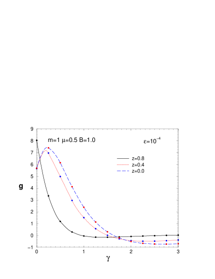
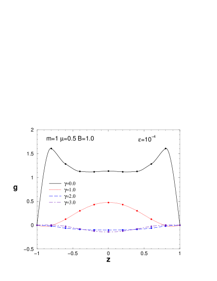
Figure 2: Function $g(\gamma,z)$ for $\mu=0.5$ and $B=1.0$. On left – versus $\gamma$ for fixed values of $z$ and on right – versus $z$ for a few fixed values of $\gamma$.

We would like to remark the striking stability of the results with respect to $N_{\gamma}$ the number of grid points on $\gamma$. The value $N_{\gamma}=12$ used in our calculations was only for drawing purposes. In fact, the accuracy in calculating the eigenvalues in table 1 is reached with $N_{\gamma}=1$. This means that on the practical point of view our method leads to an equation whose solution is mostly one-dimensional and a number of grid points of the order of 10 on $z$-variable is enough to ensure an accuracy better than $10^{-4}$.

The weight function $g$ for a system with $\mu=0.5$ and $B=1.0$ is plotted in fig. 2. It has been obtained with $\varepsilon=10^{-4}$ and the same grid parameters than in table 1. Its $\gamma$-dependence is not monotonous and has a nodal structure; the $z$-variation is also non trivial. We have remarked a strong dependence of $g(\gamma,z)$ relative to values of the $\varepsilon$ parameter smaller than $\sim 10^{-4}$, in contrast to high stability of corresponding eigenvalues. However the corresponding BS amplitude $\Phi$ and LF wave function $\psi$, obtained from $g(\gamma,z)$ by the integrals (2) and (14), show the same strong stability as the eigenvalues.

The BS amplitude in Minkowski space in the rest frame $\vec{p}=0$ is shown in fig. 3. The $k$-dependence is rather smooth but the $k_{0}$-dependence, due to poles of the propagators in (1), exhibits a singular behaviour at
$k_{0}=\pm\left(\varepsilon_{k}\pm\frac{M}{2}\right)$, i.e. moving with $\vec{k}$ and $M$.

Note that our solution gives also the BS amplitude in Euclidean space, by substituting in (2) $k_{0}=ik_{4}$. The Euclidean BS amplitude $\Phi_{E}(k_{4},k)$ was found in this way in LC05 . It is indistinguishable from the one obtained by a direct solution of the Wick-rotated BS equation.

The corresponding LF wave function $\psi(k_{\perp},x)$ is shown in fig. 4. It is very similar to the LF wave functions displayed in ref. mariane , though they obey different dynamical equations. It has a simpler structure than $g(\gamma,z)$ in both arguments.

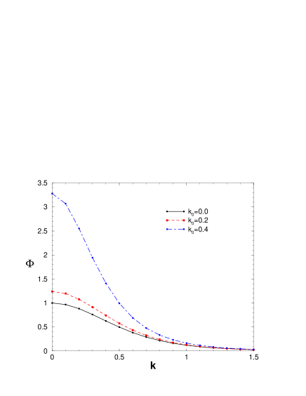
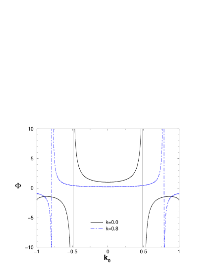
Figure 3: BS amplitude $\Phi(k_{0},k)$ for $\mu=0.5$ and $B=1.0$. On left versus $k$ for fixed values of $k_{0}$ and on right versus $k_{0}$ for a few fixed values of $k$.

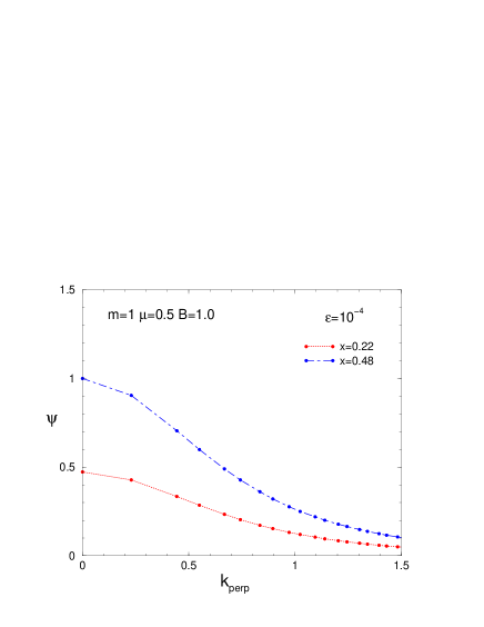
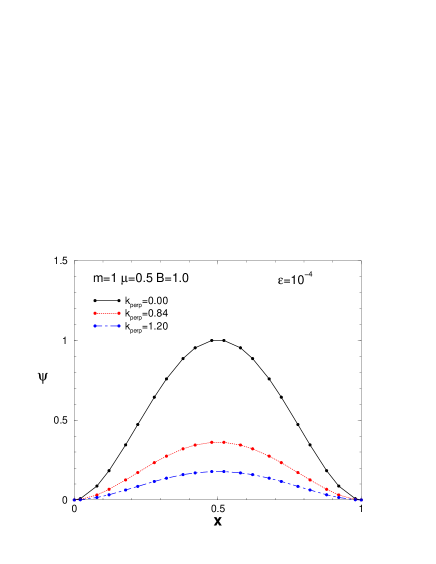
Figure 4: Wave function $\psi(k_{\perp},x)$ for $\mu=0.5$ and $B=1.0$. On left versus $k_{\perp}$ for fixed values of $x$ and on right versus $x$ for a few fixed values of $k_{\perp}$.

5 Conclusion

We have developed a method for solving the Bethe-Salpeter equation in the Minkowski space, i.e. without making use of the Wick rotation.

The method is based on an integral transform of the original equation which removes its singularities. It is motivated by the LF projection (6) of the BS amplitude.

The transformed equation is formulated in terms of the weight function of the Nakanishi integral representation nak63 , from which the original BS amplitude both in Minkowski and Euclidean spaces as well as corresponding LF wave function can be easily reconstructed.

The equation has been obtained for scalar particles and applied to the ladder kernel. For zero-mass exchange the Wick-Cutkosky model is derived. For massive exchange, numerical solutions have been found. The binding energies are in full agreement with the preceding results obtained in the Euclidean space. The singular BS amplitude in Minkowski space has been displayed.

Calculation for the ladder exchange confirms the validity of our approach. Our method can be used for an arbitrary kernel, given by a Feynman graph. In the following paper ckII it is applied to solve the BS equation with the cross-box kernel.

The method can be generalized to non-zero angular momentum and, presumably, to the fermion case. A relation similar to (6) between the BS amplitude and LF wave function for the two-nucleon system is discussed in cdkm ; bbbd .

Appendix A Derivation of equation (2)

We substitute in equation (1) the BS amplitude in the form (2) and apply to both sides the transformation (6). For the left-hand side this gives:

$$\psi=\frac{1}{\pi}\int_{-1}^{1}dz^{\prime}\int_{0}^{\infty}d\gamma^{\prime}\int_{-\infty}^{\infty}d\beta^{\prime}$$

$$\times \frac{-i\left[1/4-(\omega\cdot k)^{2}/(\omega\cdot p)^{2}\right]g(\gamma^{\prime},z^{\prime})}{\left[\gamma^{\prime}+\kappa^{2}-k^{2}-p\cdot k\;z^{\prime}-\beta^{\prime}\Bigl{(}z^{\prime}+2\frac{(\omega\cdot k)}{(\omega\cdot p)}\Bigr{)}-i\epsilon\right]^{3}},$$

where $\beta^{\prime}=(\omega\cdot p)\beta$. As seen from (A), $\psi$ depends on three scalar products $k^{2}$, $p\cdot k$ and $\frac{\omega\cdot k}{\omega\cdot p}$. However, because of the relation

$$p\cdot k=2\frac{\omega\cdot k}{\omega\cdot p}\left(k^{2}-m^{2}+\frac{1}{4}M^{2}\right),$$

only two of them are independent. We use the LF variables (7) and express through them the scalar products:

$$k^{2} = m^{2}-\frac{k_{\perp}^{2}+m^{2}}{4x(1-x)},$$

$$p\cdot k = \frac{1}{4}(1-2x)\left(\frac{k_{\perp}^{2}+m^{2}}{x(1-x)}-M^{2}\right),$$

$$\frac{\omega\cdot k}{\omega\cdot p} = x-\frac{1}{2}.$$

By means of these relations, LF wave function (A) depends on $k_{\perp},x$.

It is convenient to introduce other notations:

$$\gamma=k_{\perp}^{2},\quad z=1-2x,\quad\kappa^{2}=m^{2}-\frac{1}{4}M^{2},$$

so that:

$$k^{2} = -\frac{(\gamma+z^{2}m^{2})}{1-z^{2}},$$

$$p\cdot k = \frac{z[\gamma+z^{2}m^{2}+(1-z^{2})\kappa^{2}]}{1-z^{2}},$$

$$\frac{\omega\cdot k}{\omega\cdot p} = -\frac{1}{2}z$$ (30)

and

$$s=\frac{4(\gamma+m^{2})}{1-z^{2}}=\frac{k_{\perp}^{2}+m^{2}}{x(1-x)}.$$ (31)

The integral (A) over $\beta^{\prime}$ is simply calculated by means of the formula:

$$\int_{-\infty}^{\infty}\frac{d\beta}{(\beta x-y-i\epsilon)^{3}}=\frac{i\pi}{y^{2}}\delta(x).$$

The result of transformation is given by eq. (14). In terms of the variables $\gamma,z$ it reads:

$$\psi(\gamma,z)=\frac{1}{8\sqrt{\pi}}\int_{0}^{\infty}\frac{(1-z^{2})g(\gamma^{\prime},z)d\gamma^{\prime}}{\Bigl{[}\gamma^{\prime}+\gamma+z^{2}m^{2}+\kappa^{2}(1-z^{2})\Bigr{]}^{2}}.$$ (32)

Apart from the factor $(1-z^{2})/(8\sqrt{\pi})$ (cancelled in the final equation) it is the left-hand side of eq. (2). Substitution of (1) and (2) in right-hand side of (2) results in the right-hand side of eq. (2).

The function $\psi(\gamma,z)$ in eq. (32) is the usual two-body LF wave function. In terms of variables $k_{\perp},x$ it obtains the form (14). The normalization integral reads:

$$N_{2} = \frac{1}{(2\pi)^{3}}\int\psi^{2}(k_{\perp},x)\;\frac{d^{2}k_{\perp}dx}{2x(1-x)}$$

$$= \frac{1}{(2\pi)^{3}}\int\psi^{2}(\gamma,z)\;\frac{\pi d\gamma dz}{1-z^{2}}.$$

We would like to emphasize the mathematical nature of the above transformation. Namely, the integral transformation (6), applied to BS function (2), obtains the form (A). The function $\psi$ there still depends on the variables $k^{2},p\cdot k$, like the initial BS function, but it is not singular. However, the variables $\gamma^{\prime},z^{\prime}$ in the integrand $g(\gamma^{\prime},z^{\prime})$ and $k^{2},p\cdot k$ in $\psi$ run over different domains: $0\leq\gamma^{\prime}<\infty$, $-1\leq z^{\prime}\leq 1$, whereas $-\infty<k^{2}\leq 0$, $-\infty<p\cdot k<\infty$. By eqs. (A) we replace the variables $k^{2},p\cdot k$ by the new ones $\gamma,z$, which, by construction, vary in the same domain as $\gamma^{\prime},z^{\prime}$. In these variables eq. (A) obtains the form (32), where the functions $g(\gamma,z)$ and $\psi(\gamma,z)$ before and after integration are now defined in the same domain, like it normally takes place in the integral equations. Therefore, in new variables $\gamma,z$ we will find equation for $g(\gamma,z)$ in the domain of its definition.

We separate the factor $(1-z^{2})/(8\sqrt{\pi})$, i.e. introduce $\tilde{\psi}$ related to $\psi$ as $\psi(\gamma,z)=(1-z^{2})\tilde{\psi}(\gamma,z)/(8\sqrt{\pi})$. That is:

$$\tilde{\psi}(\gamma,z)=\int_{0}^{\infty}\frac{g(\gamma^{\prime},z)d\gamma^{\prime}}{\Bigl{[}\gamma^{\prime}+\gamma+z^{2}m^{2}+\kappa^{2}(1-z^{2})\Bigr{]}^{2}}.$$ (33)

Eq. (2) can be rewritten for the function $\tilde{\psi}$:

$$\tilde{\psi}(\gamma,z)=\int_{0}^{\infty}d\gamma^{\prime}\int_{-1}^{1}dz^{\prime}\;H(\gamma,z;\gamma^{\prime},z^{\prime})\tilde{\psi}(\gamma^{\prime},z^{\prime}),$$ (34)

where

$$H(\gamma,z;\gamma^{\prime},z^{\prime})=\int_{0}^{\infty}d\gamma^{\prime\prime}V(\gamma,z;\gamma^{\prime\prime},z^{\prime})h(\gamma^{\prime\prime},\gamma^{\prime},z^{\prime})$$

and $h(\gamma^{\prime\prime},\gamma^{\prime},z^{\prime})$ is the kernel of the operator providing the relation inverse to eq. (33), namely:

$$g(\gamma,z)=\int_{0}^{\infty}d\gamma^{\prime}h(\gamma,\gamma^{\prime},z)\tilde{\psi}(\gamma^{\prime},z).$$

Numerical calculation of the kernel $h(\gamma,\gamma^{\prime},z)$, then finding $H(\gamma,z;\gamma^{\prime},z^{\prime})$ and solving equation in the form (34) give the same results as for (2).

Appendix B Derivation of the ladder LF equation (15)

We take, for a moment, $\omega=(1,0,0,-1)$, introduce the variables $\vec{k^{\prime}}_{\perp}=(k^{\prime}_{x},k^{\prime}_{y})$, $k^{\prime}_{\pm}=k^{\prime}_{0}\pm k^{\prime}_{z}$ and represent the integration volume $d^{4}k^{\prime}$ in the right-hand side of eq. (2) as

$$d^{4}k^{\prime}=\frac{1}{2}d^{2}k^{\prime}_{\perp}dk^{\prime}_{+}dk^{\prime}_{-}=d^{2}k^{\prime}_{\perp}dx^{\prime}\;(\omega\cdot p)d\beta^{\prime},$$

where $x^{\prime}$ is defined in (7) and $k^{\prime}_{-}=\omega_{-}\beta^{\prime}$ (with $\omega_{-}=2$). For arbitrary $\omega$ eq. (2) obtains the form:

$$\int d\beta\Phi(k+\beta\omega,p)=\int d\beta G_{0}^{(12)}(k+\beta\omega,p)\frac{d^{2}k^{\prime}_{\perp}dx^{\prime}}{(2\pi)^{4}}$$

$$\times iK(k+\beta\omega,k^{\prime}+\beta^{\prime}\omega,p)\Phi(k^{\prime}+\beta^{\prime}\omega,p)(\omega\cdot p)d\beta^{\prime}$$ (35)

According to eq. (1), BS amplitude $\Phi(k,p)$ contains as a factor the product of two free propagators (1). We separate the propagators, i.e., introduce the vertex function $\Gamma(k,p)$:

$$\Phi(k,p)=G^{(12)}_{0}(k,p)\Gamma(k,p)$$ (36)

and substitute (36) in the right-hand side of (B).

In order to derive LF equation (15) from (B), we should, integrating over $\beta^{\prime}$, neglect the singularities of $\Gamma(k^{\prime}+\beta^{\prime}\omega,p)$, i.e. deal with $\Gamma$ vs. $\beta^{\prime}$ as with a constant. That is, we will extract $\Gamma$ from integral over $\beta^{\prime}$ and introduce it back. This allows the following approximate transformation of the right-hand side of (B) (for shortness we show only the $\beta,\beta^{\prime}$-dependence and don’t show integration over $d^{2}k^{\prime}_{\perp}dx^{\prime}$):

$$\int d\beta G_{0}^{(12)}(\beta)K(\beta,\beta^{\prime})G_{0}^{(12)}(\beta^{\prime})\Gamma(\beta^{\prime})d\beta^{\prime}\approx$$

$$\Gamma\int d\beta G_{0}^{(12)}(\beta)K(\beta,\beta^{\prime})G_{0}^{(12)}(\beta^{\prime})d\beta^{\prime}=$$

$$\Gamma\frac{\int G_{0}^{(12)}(\beta^{\prime})d\beta^{\prime}}{\int G_{0}^{(12)}(\beta^{\prime})d\beta^{\prime}}\int d\beta G_{0}^{(12)}(\beta)K(\beta,\beta^{\prime})G_{0}^{(12)}(\beta^{\prime})d\beta^{\prime}\approx$$

$$\frac{\int G_{0}^{(12)}(\beta^{\prime})\Gamma(\beta^{\prime})d\beta^{\prime}}{\int G_{0}^{(12)}(\beta^{\prime})d\beta^{\prime}}\int d\beta G_{0}^{(12)}(\beta)K(\beta,\beta^{\prime})G_{0}^{(12)}(\beta^{\prime})d\beta^{\prime}=$$

$$\frac{\int d\beta G_{0}^{(12)}(\beta)K(\beta,\beta^{\prime})G_{0}^{(12)}(\beta^{\prime})d\beta^{\prime}}{\int G_{0}^{(12)}(\beta^{\prime})d\beta^{\prime}}\int\Phi(\beta^{\prime})d\beta^{\prime}\phantom{=}$$

The integral $\int\Phi(\beta^{\prime})d\beta^{\prime}$ is understood as
$\int_{-\infty}^{\infty}\Phi(k^{\prime}+\beta^{\prime}\omega,p)d\beta^{\prime}$ and it is related by (6) to the LF wave function (as well as the left-hand side of (B)). With explicit expression (1) for $G_{0}^{(12)}$ we find:

$$(\omega\cdot p)\int_{-\infty}^{\infty}d\beta G_{0}^{(12)}(k+\beta\omega,p)=\frac{-\pi i}{x(1-x)(s-M^{2})},$$

where $s$ is defined in (31). With explicit expression (16) for $K$ we obtain:

$$(\omega\cdot p)^{2}\int_{-\infty}^{\infty}d\beta G_{0}^{(12)}(k+\beta\omega,p)K(k+\beta\omega,k^{\prime}+\beta^{\prime}\omega,p)$$

$$\times G_{0}^{(12)}(k^{\prime}+\beta^{\prime}\omega,p)d\beta^{\prime}=$$

$$\frac{-\pi i}{x(1-x)(s-M^{2})}\;\left(-4m^{2}V_{LF}^{(L)}\right)\;\frac{-\pi i}{x^{\prime}(1-x^{\prime})(s^{\prime}-M^{2})},$$

where $V$ is the standard LF ladder kernel (see e.g. cdkm ):

$$V_{LF}^{(L)}(\vec{k}^{\prime}_{\perp},x^{\prime};\vec{k}_{\perp},x,M^{2})=$$

$$-\frac{4\pi\alpha\theta(x^{\prime}-x)}{(x^{\prime}-x)(s_{a}-M^{2})}-\frac{4\pi\alpha\theta(x-x^{\prime})}{(x-x^{\prime})(s_{b}-M^{2})},$$ (37)

and

$$s_{a} = \frac{\vec{k}^{2}_{\perp}+m^{2}}{x}+\frac{(\vec{k^{\prime}}_{\perp}-\vec{k}_{\perp})^{2}+\mu^{2}}{x^{\prime}-x}+\frac{\vec{k^{\prime}}^{2}_{\perp}+m^{2}}{1-x^{\prime}},$$

$$s_{b} = \frac{\vec{k^{\prime}}^{2}_{\perp}+m^{2}}{x^{\prime}}+\frac{(\vec{k^{\prime}}_{\perp}-\vec{k}_{\perp})^{2}+\mu^{2}}{x-x^{\prime}}+\frac{\vec{k}^{2}_{\perp}+m^{2}}{1-x}.$$

In this way we derive the equation (15) with the kernel (B).

Appendix C Calculation of the kernel $V^{(L)}(\gamma,z;\gamma^{\prime},z^{\prime})$, eq. (17)

With the ladder kernel (16) the integral (13) obtains the form:

$$I(k,p) = \frac{-i16\pi m^{2}\alpha}{(2\pi)^{4}}\int\frac{d^{4}k^{\prime}}{\Bigl{[}(k^{\prime}-k)^{2}-\mu^{2}+i\epsilon\Bigr{]}}$$

$$\times \frac{1}{\Bigl{[}{k^{\prime}}^{2}+p\cdot k^{\prime}\;z^{\prime}-\kappa^{2}-\gamma^{\prime}+i\epsilon\Bigr{]}^{3}},$$

where we put $g^{2}=16\pi m^{2}\alpha$. Using the formula:

$$\frac{1}{ab^{3}}=\int_{0}^{1}\frac{3v^{2}dv}{[a(1-v)+bv]^{4}}$$

and replacing $k^{\prime}$ by new integration variable $q$ by the relation:

$$k^{\prime}=q+(1-v)k-\frac{1}{2}vz^{\prime}p,$$

we get

$$I(k,p) = \frac{-i16\pi m^{2}\alpha}{(2\pi)^{4}}\int_{0}^{1}3v^{2}dv\int\frac{d^{4}q}{\left[{q}^{2}+A(p,k)+i\epsilon\right]^{4}}$$ (38)

$$= \frac{\alpha m^{2}}{2\pi}\int_{0}^{1}\frac{v^{2}dv}{[A(p,k)+i\epsilon]^{2}}$$

with

$$A(p,k) = v(1-v)(k^{2}+p\cdot k\;z^{\prime})-vm^{2}$$

$$+ \frac{1}{4}v(1-v{z^{\prime}}^{2})M^{2}-(1-v)\mu^{2}-v\gamma^{\prime}.$$

Now we make in (38) the replacement $k\to k+\beta\omega$ and substitute it in (12). Scalar products $k^{2},p\cdot k$ and also $(\omega\cdot k)/(\omega\cdot p)$, which the kernel depends on, are expressed through the variables $\gamma,z$ by eqs. (A). Since

$$A(p,k+\beta\omega)=A(p,k)+\beta^{\prime}v(1-v)(z^{\prime}-z)$$

with $\beta^{\prime}=(\omega\cdot p)\beta$, we obtain:

$$V^{(L)}(\gamma,z;\gamma^{\prime},z^{\prime})=\frac{-i\alpha m^{2}}{2\pi^{2}}$$

$$\times\int_{0}^{1}v^{2}dv\int_{-\infty}^{\infty}\frac{d\beta^{\prime}}{\Bigl{[}A(p,k)+\beta^{\prime}v(1-v)(z^{\prime}-z)+i\epsilon\Bigr{]}^{2}}$$

$$\times\frac{1}{\left[k^{2}+p\cdot k-\kappa^{2}+(1-z)\beta^{\prime}+i\epsilon\right]}$$

$$\times\frac{1}{\left[k^{2}-p\cdot k-\kappa^{2}-(1+z)\beta^{\prime}+i\epsilon\right]}.$$ (39)

Both $z$ and $z^{\prime}$ vary from $-1$ to 1. We consider two cases: (i) $z^{\prime}<z$ and (ii) $z<z^{\prime}$. In the case (i) the factor $\Bigl{(}z^{\prime}-z\Bigr{)}$ is negative and the (second order) pole in the variable $\beta^{\prime}$ of the factor $1/\Bigl{[}A+\beta^{\prime}v(1-v)(z^{\prime}-z)+i\epsilon\Bigr{]}^{2}$ in (C) is at the value $\beta^{\prime}\sim\ldots+i\epsilon$. We close the contour in the lower half-plane, i.e, take the residue at the pole of the first propagator:

$$\beta^{\prime}=-\frac{k^{2}+p\cdot k-\kappa^{2}}{1-z}-i\epsilon.$$

This gives:

$$V^{(L)}(\gamma,z;\gamma^{\prime},z^{\prime})=W(\gamma,z;\gamma^{\prime},z^{\prime})$$

with

$$W(\gamma,z;\gamma^{\prime},z^{\prime})=\frac{\alpha m^{2}(1-z)^{2}}{2\pi\Bigl{[}\gamma+z^{2}m^{2}+(1-z^{2})\kappa^{2}\Bigr{]}}\int_{0}^{1}\frac{v^{2}dv}{D^{2}}$$ (40)

and

$$D = v(1-v)(1-z^{\prime})\gamma+v(1-z)\gamma^{\prime}$$

$$+ v(1-z)(1-z^{\prime})\Bigl{[}1+z(1-v)+vz^{\prime}\Bigr{]}\kappa^{2}$$

$$+ v\Bigl{[}(1-v)(1-z^{\prime})z^{2}+v{z^{\prime}}^{2}(1-z)\Bigr{]}m^{2}$$

$$+ (1-v)(1-z)\mu^{2}.$$

In the case (ii) the factor $(z^{\prime}-z)$ is positive and the pole in the variable $\beta^{\prime}$ of the factor $1/\Bigl{[}A+\beta^{\prime}v(1-v)(z^{\prime}-z)+i\epsilon\Bigr{]}^{2}$ is at the value $\beta^{\prime}\sim\ldots-i\epsilon$. We close the contour in the upper half-plane, i.e, take the residue at the pole of the second propagator:

$$\beta^{\prime}=\frac{k^{2}-p\cdot k-\kappa^{2}}{1+z}+i\epsilon.$$

This gives:

$$V^{(L)}(\gamma,z;\gamma^{\prime},z^{\prime})=W(\gamma,-z;\gamma^{\prime},-z^{\prime}).$$

with $W$ defined in (40). The integral for $W$ is calculated analytically. In this way, we obtain eqs. (17), (18) for the ladder kernel in the equation (2).

References

(1)
E.E. Salpeter, H.A. Bethe, Phys. Rev. 84, 1232 (1951).
(4) T. Nieuwenhuis and J.A. Tjon, Few-Body Systems
21, 167 (1996).
(5)G.V. Efimov, Few-Body Syst., 33, 199 (2003).
(6) K. Kusaka, A.G. Williams, Phys. Rev. D 51, 7026 (1995);
K. Kusaka, K. Simpson, A.G. Williams, Phys. Rev. D 56, 5071
(1997).
(7)
N. Nakanishi, Phys. Rev. 130, 1230 (1963); Graph Theory
and Feynman Integrals (Gordon and Breach, New York, 1971).
(8) S.G. Bondarenko, V.V. Burov, A.M. Molochkov,
G.I. Smirnov and H. Toki, Prog. in Part. and Nucl. Phys., 48, 449 (2002).
(9)
J.H.O. Sales, T. Frederico, B.V. Carlson and P.U. Sauer,
Phys. Rev. C 61, 044003 (2000);
T. Frederico, J.H.O. Sales, B.V. Carlson and P.U. Sauer, Nucl.
Phys. A 737, 260 (2004).
(10)
J. Carbonell, B. Desplanques, V.A. Karmanov and
J.-F. Mathiot, Phys. Reports, 300, 215 (1998).
(11)
J. Carbonell and V.A. Karmanov, Eur. Phys. J. A 27 (1), 11
(2006); hep-th/0505262.
(12) R.E. Cutkosky, Phys. Rev. 96, 1135 (1954).
(13) M. Mangin-Brinet and J. Carbonell,
Phys. Lett., B 474, 237 (2000).
(14)
V.A. Karmanov, Nucl. Phys. B 166, 378 (1980).
(15)
M. Sawicki, Phys. Rev. D 32, 2666 (1985); D 33, 1103
(1986).
(16)
G. L. Payne, Models and Methods in Few-Body Physics, edited by
L.S. Ferreira et al., Lect. Notes in Phys. Vol. 93 (Springer
Berlin, 1987) 64.
(17) V.I. Korobov, private communication, 2004.
(18)
V.A. Karmanov and J. Carbonell, Proceedings of Workshop ”Light-Cone
QCD and Nonperturbative Hadron Physics”, Cairns, Australia, July
7-15, 2005, to be published in Nucl. Phys. B, 2006;
nucl-th/0510051.
(19) S.G. Bondarenko, V.V. Burov, M. Beyer and S.M. Dorkin, Few-Body Syst.,
26, 185 (1999).