Cross-ladder effects in Bethe-Salpeter and Light-Front equations

Abstract

Bethe-Salpeter (BS) equation in Minkowski space for scalar particles is solved for a kernel given by a sum of ladder and cross-ladder exchanges. The solution of corresponding Light-Front (LF) equation, where we add the time-ordered stretched boxes, is also obtained. Cross-ladder contributions are found to be very large and attractive, whereas the influence of stretched boxes is negligible. Both approaches – BS and LF – give very close results.

1 Introduction

In a preceding paper ckI we have proposed a new method for solving the BS equation BS in the Minkowski space. Our approach does not make use of the transform to the Euclidean space (Wick rotation) and is applicable to an arbitrary interaction kernel. This method was first applied in ckI to obtain the ladder solutions of a scalar model with interaction Lagrangian ${\cal L}_{WC}=g\phi^{2}\chi$. For massless exchange we reproduced analytically the Wick-Cutkosky equation WICK_54_CUTKOSKY_PR96_54 . For massive ladder exchange our numerical results coincide with ones found in previous works based on the Wick rotation.

In the present paper we solve the BS and LF equations with a kernel given by a sum of ladder and cross-ladder graphs. This constitutes the first calculation of cross-ladder effects in both equations. We consider scalar constituents in the state with zero total angular momentum. BS equation with ladder kernel was solved in Minkowski space in KW .

Non ladder effects, within the same model, using Feynman-Schwinger representation, were considered in ref. NT_PRL_96 . In this work the full set of all irreducible cross-ladder graphs in a bound state calculation was included. In ADT the effect of the cross-ladder graphs in the BS framework was estimated with the kernel represented through a dispersion relation. Non ladder self-energy effects in LF equation have been incorporated in Ji ; Adam .

The plan of the paper is the following. In section 2 we sketch the method used in ckI for solving the BS equation and find the kernel corresponding to the cross-ladder Feynman amplitude. In section 3 we remind the LF equation, obtain the LF cross-ladder kernel and incorporate also two stretched box graphs. Numerical results are given in section 4. Section 5 contains some concluding remarks. Technical details of the derivation are given in appendices A, B and C.

2 Cross-ladder kernel in BS equation

The method for solving the BS equation proposed in our previous work ckI is based on projecting the original equation:

$$\Phi(k,p) = \frac{i^{2}}{\left[(\frac{p}{2}+k)^{2}-m^{2}+i\epsilon\right]\left[(\frac{p}{2}-k)^{2}-m^{2}+i\epsilon\right]}$$ (1)

$$\times \int\frac{d^{4}k^{\prime}}{(2\pi)^{4}}iK(k,k^{\prime},p)\Phi(k^{\prime},p)$$

on the LF plane, i.e in applying to both sides of (1) the integral transform, which for the left-hand side reads

$$\int_{-\infty}^{\infty}\Phi(k+\beta\omega,p)d\beta$$

and similarly for the full right-hand side. Here $\omega$ is an arbitrary four-vector with $\omega^{2}=0$. This transformation eliminates the singularities of the BS equation. The BS amplitude in the transformed equation is then written in terms of the Nakanishi integral representation nakanishi , which for zero angular momentum reads:

$$\Phi(k,p) = \frac{-i}{\sqrt{4\pi}}\int_{-1}^{1}dz^{\prime}\int_{0}^{\infty}d\gamma^{\prime}$$

$$\times \frac{g(\gamma^{\prime},z^{\prime})}{\left[\gamma^{\prime}+m^{2}-\frac{1}{4}M^{2}-k^{2}-p\cdot k\;z^{\prime}-i\epsilon\right]^{3}}$$

The equation satisfied by the weight function $g(\gamma,z)$ was derived in ckI and has the form:

$$\int_{0}^{\infty}\frac{g(\gamma^{\prime},z)d\gamma^{\prime}}{\Bigl{[}\gamma^{\prime}+\gamma+z^{2}m^{2}+(1-z^{2})\kappa^{2}\Bigr{]}^{2}}=$$

$$\int_{0}^{\infty}d\gamma^{\prime}\int_{-1}^{1}dz^{\prime}\;V(\gamma,z;\gamma^{\prime},z^{\prime})g(\gamma^{\prime},z^{\prime}),$$ (3)

where $V$ is a kernel given in terms of the BS interaction kernel $iK$ by

$$V(\gamma,z;\gamma^{\prime},z^{\prime})=\frac{\omega\cdot p}{\pi}\int_{-\infty}^{\infty}\frac{-iI(k+\beta\omega,p)d\beta}{\left[(\frac{p}{2}+k+\beta\omega)^{2}-m^{2}+i\epsilon\right]}$$

$$\phantom{V(\gamma,z;\gamma^{\prime},z^{\prime})}\times\frac{1}{\left[(\frac{p}{2}-k-\beta\omega)^{2}-m^{2}+i\epsilon\right]},$$ (4)

$$I(k,p)=\int\frac{d^{4}k^{\prime}}{(2\pi)^{4}}\frac{iK(k,k^{\prime},p)}{\left[{k^{\prime}}^{2}+p\cdot k^{\prime}z^{\prime}-\gamma^{\prime}-\kappa^{2}+i\epsilon\right]^{3}}.$$ (5)

The bound state mass $M$ enters through the parameter

$$\kappa^{2}=m^{2}-\frac{1}{4}M^{2}.$$

Equation (2) is equivalent to the initial BS equation (1) and provides, for a given kernel $K(k,k^{\prime},p)$, the same bound state mass $M$. Once $g(\gamma,z)$ is known, the BS amplitude can be restored by eq. (2). Corresponding LF wave function $\psi(k_{\perp},x)$ can be easily obtained by

$$\psi(k_{\perp},x)=\frac{1}{\sqrt{4\pi}}\int_{0}^{\infty}\frac{x(1-x)g(\gamma^{\prime},1-2x)d\gamma^{\prime}}{\Bigl{[}\gamma^{\prime}+k_{\perp}^{2}+m^{2}-x(1-x)M^{2}\Bigr{]}^{2}}.$$ (6)

In ckI for the ladder exchange

$$K^{(L)}(k,k^{\prime},p)=\frac{-g^{2}}{(k-k^{\prime})^{2}-\mu^{2}+i\epsilon}$$

we calculated the integrals (2), (5) for the kernel $V$ and solved equation (2). Derivation of $V$ for the cross-ladder kernel is quite similar but more lengthy, since the kernel itself is more complicated.

Figure 1: Feynman cross graph.

The cross-ladder BS kernel is shown in fig. 1. On mass-shell it depends on two variables: $s=(p_{1}+p_{2})^{2}$ and $t=(p_{1}-p^{\prime}_{1})^{2}$. The kernel $K$ in the BS equation (1) is off-mass shell. It depends also on $p_{i}^{2}$, i.e., on six scalar variables in general: $s,t,p_{1}^{2},p_{2}^{2},{p^{\prime}_{1}}^{2},{p^{\prime}_{2}}^{2}$. One can also construct six variables, using the total momentum $p$ and relative momenta $k,k^{\prime}$:

$$p^{2},\quad k^{2},\quad{k^{\prime}}^{2},\quad k\cdot k^{\prime},\quad k\cdot p,\quad k^{\prime}\cdot p,$$

where

$$p=p_{1}+p_{2}=p^{\prime}_{1}+p^{\prime}_{2},\quad k=\frac{1}{2}(p_{1}-p_{2}),\quad k^{\prime}=\frac{1}{2}(p^{\prime}_{1}-p^{\prime}_{2}).$$

In the bound state problem the value of $p^{2}$ is fixed: $p^{2}=M^{2}$.

The amplitude corresponding to the diagram in fig. 1 reads:

$$K^{(CL)}(k,k^{\prime},p)=$$ (7)

$$\frac{-ig^{4}}{(2\pi)^{4}}\int\frac{1}{[{p^{\prime\prime}}^{2}-m^{2}+i\epsilon][(p^{\prime}_{2}-p_{1}+p^{\prime\prime})^{2}-m^{2}+i\epsilon]}$$

$$\times \frac{d^{4}p^{\prime\prime}}{[(p_{1}-p^{\prime\prime})^{2}-\mu^{2}+i\epsilon][(p^{\prime}_{1}-p^{\prime\prime})^{2}-\mu^{2}+i\epsilon]}.$$

We have first to calculate this expression, substitute the result in (5), then in (2) and find in this way the cross-ladder contribution to the kernel $V(\gamma,z;\gamma^{\prime},z^{\prime})$ in equation (2).

The full kernel – including ladder and cross-ladder graphs – will be written in the form:

$$V(\gamma,z;\gamma^{\prime},z^{\prime})=V^{(L)}(\gamma,z;\gamma^{\prime},z^{\prime})+V^{(CL)}(\gamma,z;\gamma^{\prime},z^{\prime}).$$

The ladder kernel $V^{(L)}$ was found in ckI . The cross-ladder contribution $V^{(CL)}$ is calculated in appendix A.

3 Ladder, cross-ladder and stretched-box kernel in LF equation

We would like to compare the results obtained in the BS approach with the equivalent ones found in Light-Front Dynamics (LFD). For this aim we precise in what follows the LF equation and derive the corresponding kernel. In the well-known variables $\vec{k}_{\perp}$ and $x$ the LF equation reads (see e.g. cdkm ):

$$\left(\frac{\vec{k}^{2}_{\perp}+m^{2}}{x(1-x)}-M^{2}\right)\psi(\vec{k}_{\perp},x)=$$ (8)

$$-\frac{m^{2}}{2\pi^{3}}\int\psi(\vec{k}^{\prime}_{\perp},x^{\prime})V_{LF}(\vec{k}^{\prime}_{\perp},x^{\prime};\vec{k}_{\perp},x,M^{2})\frac{d^{2}k^{\prime}_{\perp}dx^{\prime}}{2x^{\prime}(1-x^{\prime})}\ .$$

Figure 2: Ladder LFD graphs.

The two time-ordered ladder graphs are shown in fig. 2. The corresponding kernel has the form:

$$V^{(L)}_{LF}(\vec{k}^{\prime}_{\perp},x^{\prime};\vec{k}_{\perp},x,M^{2})=$$

$$-\frac{4\pi\alpha\theta(x^{\prime}-x)}{(x^{\prime}-x)(s_{a}-M^{2})}-\frac{4\pi\alpha\theta(x-x^{\prime})}{(x-x^{\prime})(s_{b}-M^{2})},$$ (9)

where

$$s_{a}=\frac{\vec{k}^{2}_{\perp}+m^{2}}{x}+\frac{(\vec{k^{\prime}}_{\perp}-\vec{k}_{\perp})^{2}+\mu^{2}}{x^{\prime}-x}+\frac{\vec{k^{\prime}}^{2}_{\perp}+m^{2}}{1-x^{\prime}}$$

and

$$s_{b}=\frac{\vec{k^{\prime}}^{2}_{\perp}+m^{2}}{x^{\prime}}+\frac{(\vec{k^{\prime}}_{\perp}-\vec{k}_{\perp})^{2}+\mu^{2}}{x-x^{\prime}}+\frac{\vec{k}^{2}_{\perp}+m^{2}}{1-x}.$$

$V_{1}$

$V_{2}$

$V_{3}$

$V_{4}$

$V_{5}$

$V_{6}$

Figure 3: Cross LFD graphs.

$V_{7}$

$V_{8}$

Figure 4: Stretched boxes.

The six different cross-ladder diagrams are shown in fig. 3. They have order $\alpha^{2}$. In addition, and in the same order $\alpha^{2}$, there are two time-ordered irreducible graphs with two mesons in the intermediate state (stretched boxes). They are shown in fig. 4. The full LFD kernel – including ladder, cross-ladder and stretched-box graphs – will be written in the form:

$$V_{LF}(\vec{k}^{\prime}_{\perp},x^{\prime};\vec{k}_{\perp},x,M^{2})=V_{LF}^{(L)}+V_{LF}^{(CL)}+V_{LF}^{(SB)}.$$

The term $V_{LF}^{(L)}$ is given by (3) and

$$V_{LF}^{(CL)}=\sum_{i=1}^{6}V_{i},\quad V_{LF}^{(SB)}=\sum_{i=7,8}V_{i}$$ (10)

are calculated in appendices B and C correspondingly.

4 Numerical results

We have solved numerically the BS equation in the form (2) and the LF equation (8) both for the ladder (L) and ladder+cross-ladder (L+CL) kernels. In the case of the LF equation (8) we added also the stretched box contributions (L+CL+SB) with two intermediate mesons shown in fig. 4. These stretched box contributions, as well as those with any number of intermediate mesons, are generated by iterations of the ladder BS kernel and are thus implicitly included in the BS approach.

The numerical procedure, based in the spline expansion of the solution, is similar to the one used in ckI . By expanding the solution $g(\gamma,z)$ on a spline basis we obtain a matrix equation:

$$\lambda B(M)g=A(M,\alpha)g.$$ (11)

Like in ckI , the matrix $B(M)$ was regularized by adding to its diagonal a small value $\varepsilon\sim 10^{-4}\div 10^{-12}$ and we have checked the stability of the eigenvalus relative to $\varepsilon$. The difference with respect to the ladder kernel is that the coupling constant $\alpha$ does not appear linearly in the right-hand side of (11). For a fixed mass $M$, the eigenvalue $\lambda$ is calculated for different values of $\alpha$ and the value corresponding to $\lambda=1$ can be easily extrapolated from the almost linear behaviour of $\lambda(\alpha)$.

Table 1: Coupling constant $\alpha$ for given values of the binding energy $B$ and exchanged mass $\mu=0.5$ calculated with BS and LF equations for the ladder (L), ladder +cross-ladder (L+CL) and (in LFD) for the ladder +cross-ladder +stretched-box (L+CL+SB) kernels.

B	BS(L)	BS (L+CL)	LF (L)	LFD (L+CL)	LFD (L+CL+SB)
0.01	1.44	1.21	1.46	1.23	1.21
0.05	2.01	1.62	2.06	1.65	1.62
0.10	2.50	1.93	2.57	2.01	1.97
0.20	3.25	2.42	3.37	2.53	2.47
0.50	4.90	3.47	5.16	3.67	3.61
1.00	6.71	4.56	7.17	4.97	4.91

Figure 5: Binding energy $B$ vs. coupling constant $\alpha$ for BS and LF equations with the ladder (L) kernels only and with the ladder +cross-ladder (L+CL) one for exchange mass $\mu=0.15$.

The binding energy $B$ as a function of the coupling constant $\alpha$ is shown in figures 5 and 6 for exchange masses $\mu=0.15$ and $\mu=0.5$ respectivley and unit constituent mass ($m=1$). Corresponding numerical values are given in table 1. Obtaining this results is quite a lengthy numerical task, entirely due to the evaluation of the 4-dimensional integral required in the CL kernel. This fact makes difficult – though straightforward – to reach the same accuracy than for the ladder case. The results in table 1 have been obtained with $N\approx 10$ gauss quadrature points in each integration variable ensuring an accuracy of 1%.

We see that for the same kernel – ladder or (ladder + cross-ladder) – and exchange mass – $\mu=0.15$ or $\mu=0.5$ – the binding energies obtained by BS and LFD approaches are very close to each other. The BS equation is slightly more attractive than LFD. At the same time, the results for ladder and (ladder +cross-ladder) kernels considerably differ from each other. The effect of the cross-ladder is strongly attractive. Though the stretched box graphs are included, its contribution to the binding energy is smaller than 2% and attractive as well. This agrees with the direct calculation of the stretched box contribution to the kernel done in sbk .

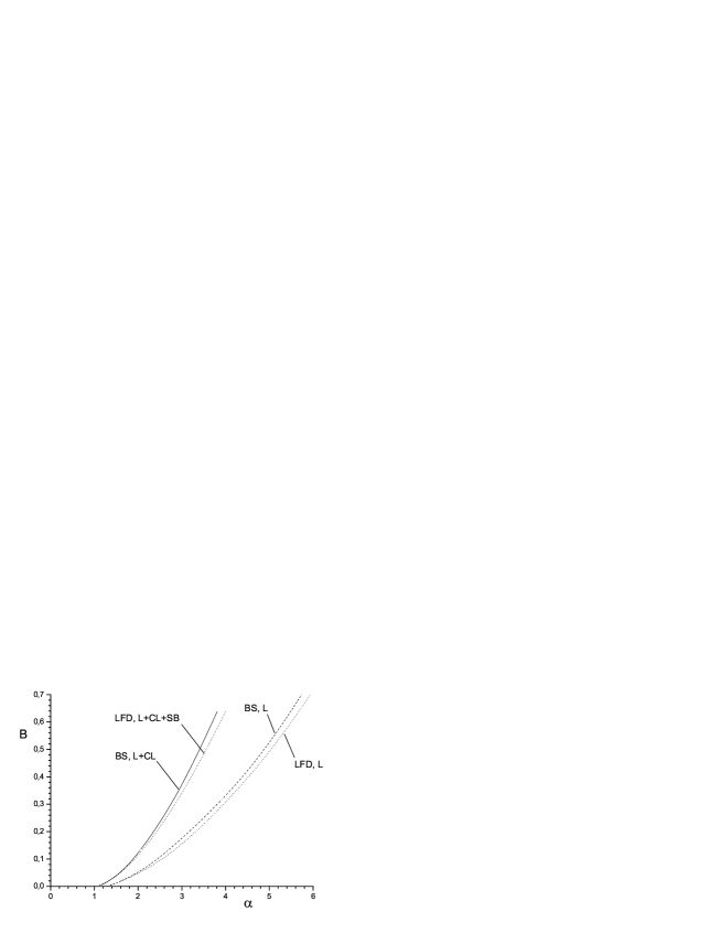
Figure 6: The same as in fig. 5 for exchange mass $\mu=0.5$ and, in addition, binding energy $B$ for LF equation with the ladder +cross-ladder +stretched box (L+CL+SB) kernel.

The zero binding limit of fig. 6 deserves some comments. It was found in mariane that for massive exchange, the relativistic (BS and LF) ladder results do not coincide with those provided by the Schrödinger equation and the corresponding non relativistic kernel (Yukawa potential) even at very small binding energies. Their differences increase with the exchanged mass $\mu$ and do not vanish in the limit $B\to 0$. We have displayed in fig. 7 a zoom of fig. 6 for small values of $B$. We see from these results that the cross ladder and stretched box diagrams reduce the differences but are not enough to cancel it.

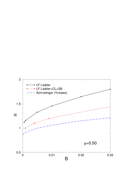
Figure 7: Zoom of figure 6 in the zero binding energy region. The ladder and (ladder +cross ladder +stretched box) results obtained with the LF equation are compared to the non relativistic ones (Schrodinger equation with Yukawa potential).

5 Conclusion

We have solved, for the first time, the BS equation for the kernel given by sum of ladder and cross-ladder exchanges. The solution was found in Minkowski space, i.e. without making use of the Wick rotation, by a new method developed in ckI .

In order to compare two different relativistic approaches, we have also solved the corresponding LF equation.

We have found that the cross-ladder contribution, relative to the ladder one, results in a strong attractive effect. The BS and LFD approaches give very close results for any kernel, with BS equation being always more attractive. These approaches differ from each other by the stretched-box diagrams with higher numbers of intermediate mesons. Our results indicate that the higher order stretched box contributions are small. This agrees with direct calculations in LFD of stretched box kernel (fig. 4) with two-meson states sbk and with calculations of the higher Fock sector contributions hk04 in the Wick-Cutkosky model. Calculation in LFD of binding energy with the stretched box contribution (L+CL+SB) and its comparison with (L+CL) also shows that the stretched box contribution is attractive but small.

The comparison of our results with those obtained in NT_PRL_96 , evaluating the binding energy $B_{all}$ for the complete set of all irreducible diagrams, shows that the effect of the considered cross ladder graphs, though being very important, represent only a small part of the total correction. Thus for $\mu=0.15$ and $\alpha=0.9$ the corresponding binding energies obtained with BS equation are $B_{L}\approx 0.035$, $B_{L+CL}\approx 0.06$ and $B_{all}\approx 0.225$.

We are aware about the only paper ADT where the separated effect of the cross-ladder in the BS framework has been estimated. The method is based on writing an approximate dispersion relation for the kernel. Our results are smaller than the ones found in this reference by a factor 3.

Appendix A Calculating BS cross-ladder

We calculate here the cross-ladder contribution $V^{(CL)}$ to the kernel in eq. (2). We start with the cross-ladder amplitude, eq. (7). Using the Feynman parametrization:

$$\frac{1}{abcd}=6\int_{0}^{1}dy_{3}\int_{0}^{1-y_{3}}dy_{2}\int_{0}^{1-y_{2}-y_{3}}dy_{1}$$

$$\times\frac{1}{[ay_{1}+by_{2}+cy_{3}+d(1-y_{1}-y_{2}-y_{3})]^{4}}$$

and calculating then the integral (7) over $p^{\prime\prime}$ in a standard way by means of the formula

$$\int\frac{d^{4}p^{\prime\prime}}{({p^{\prime\prime}}^{2}+A+i\epsilon)^{n}}=\frac{i\pi^{2}}{(n-1)(n-2)(A+i\epsilon)^{n-2}},$$ (12)

we find:

$$K^{(CL)}(k,k^{\prime},p)=$$ (13)

$$16\alpha^{2}m^{4}\int_{0}^{1}dy_{3}\int_{0}^{1-y_{3}}dy_{2}\int_{0}^{1-y_{2}-y_{3}}dy_{1}\;\frac{1}{{A^{\prime}}^{2}},$$

where $\alpha=g^{2}/(16\pi m^{2})$ and

$$A^{\prime} = {k^{\prime}}^{2}\;(y_{1}+y_{3})(1-y_{1}-y_{3})$$

$$+ k^{2}\;(y_{2}+y_{3})(1-y_{2}-y_{3})$$

$$+ k^{\prime}\cdot p\;\Bigl{(}y_{1}(1-y_{1}-y_{2})-y_{3}(y_{1}+y_{2})\Bigr{)}$$

$$- k\cdot p\;\Bigl{(}y_{2}(1-y_{1}-y_{2})-y_{3}(y_{1}+y_{2})\Bigr{)}$$

$$+ 2k\cdot k^{\prime}\;\Bigl{(}(y_{1}+y_{3})(y_{2}+y_{3})-y_{3}\Bigr{)}$$

$$+ \frac{1}{4}M^{2}\;(y_{1}+y_{2})(1-y_{1}-y_{2})$$

$$- \mu^{2}\;(1-y_{1}-y_{2})-m^{2}\;(y_{1}+y_{2})+i\epsilon.$$

Substituting the kernel (13) in eq. (5), we obtain:

$$I(k,p)=\int\frac{d^{4}k^{\prime}}{(2\pi)^{4}}\frac{iK^{(CL})(k,k^{\prime},p)}{H^{3}}=$$ (15)

$$\int_{0}^{1}dy_{3}\int_{0}^{1-y_{3}}dy_{2}\int_{0}^{1-y_{2}-y_{3}}dy_{1}\int\frac{d^{4}k^{\prime}}{(2\pi)^{4}}\frac{16i\alpha^{2}m^{4}}{{A^{\prime}}^{2}\,H^{3}},$$

where $A^{\prime}$ is given by (A) and $H$ is denominator in (5):

$$H={k^{\prime}}^{2}+p\cdot k^{\prime}\;z^{\prime}-m^{2}+\frac{1}{4}M^{2}-\gamma^{\prime}+i\epsilon.$$

Using the formula

$$\frac{1}{{A^{\prime}}^{2}\,H^{3}}=\int_{0}^{1}\frac{12y_{4}(1-y_{4})^{2}dy_{4}}{\Bigl{[}y_{4}A^{\prime}+(1-y_{4})H\Bigr{]}^{5}}$$

and shifting the integration variable $k^{\prime}$ to eliminate the terms linear in $k^{\prime}$, we calculate, again by means of eq. (12), the integral (15) over $k^{\prime}$. The result is represented in the form:

$$I(k,p)=-\frac{\alpha^{2}m^{4}}{\pi^{2}}\int\frac{\eta\,y_{4}(1-y_{4})^{2}dy_{1}dy_{2}dy_{3}dy_{4}}{\Bigl{[}A(k,p)+i\epsilon\Bigr{]}^{3}}$$ (16)

where

$$\eta=1-y_{4}[1-(1-y_{1}-y_{3})(y_{1}+y_{3})]$$ (17)

and $A(k,p)$ depends on $k,p,\gamma^{\prime},z^{\prime},y_{1-4}$. We separated the factor $\eta$ in numerator of (16) so that $A(k,p)$ be a polynomial in all the variables. We do not precise it.

Now we shift the argument $k$ of $I(k,p)$: $k\to k+\beta\omega$, substitute $I(k+\beta\omega,p)$ in eq. (2) for $V$ and replace $\beta^{\prime}=(\omega\cdot p)\beta$. In addition to the variables $\gamma^{\prime},z^{\prime}$, which enter through eq. (5), the kernel $V$ depends on three scalars $k^{2}$, $p\cdot k$ and $\frac{\omega\cdot k}{\omega\cdot p}$: $V=V(k^{2},p\cdot k,\frac{\omega\cdot k}{\omega\cdot p};\gamma^{\prime},z^{\prime})$. They vary in the intervals

$$-\infty<k^{2}\leq 0,\quad-\infty<p\cdot k<\infty,\quad-\frac{1}{2}\leq\frac{\omega\cdot k}{\omega\cdot p}\leq\frac{1}{2}$$ (18)

and satisfy the relation

$$p\cdot k=2\frac{\omega\cdot k}{\omega\cdot p}\left(k^{2}-\kappa^{2}\right).$$ (19)

Therefore, only two of them are independent. We introduce two new variables $\gamma,z$ related to the three old ones as:

$$k^{2} = -\frac{(\gamma+z^{2}m^{2})}{1-z^{2}},$$

$$p\cdot k = \frac{z[\gamma+z^{2}m^{2}+(1-z^{2})\kappa^{2}]}{1-z^{2}},$$

$$\frac{\omega\cdot k}{\omega\cdot p} = -\frac{1}{2}z.$$

With these definitions, the relation (19) turns into identity and the inequalities (18) are satisfied if $\gamma,z$ vary in the intervals $0\leq\gamma<\infty$, $-1\leq z\leq 1$. So, the kernel $V$ is now parametrized as $V=V(\gamma,z;\gamma^{\prime},z^{\prime})$, where $\gamma$ is in the same interval as $\gamma^{\prime}$ and similarly for $z,z^{\prime}$. Note that $\gamma,z$ are related to the standard LF variables $k_{\perp},x$ used in sect. 3 as $\gamma=k_{\perp}^{2}$, $z=1-2x$.

In this way we get:

$$V^{(CL)}(\gamma,z;\gamma^{\prime},z^{\prime})=\frac{-i}{\pi(1-z^{2})}\int_{-\infty}^{\infty}I\left(k+\frac{\beta^{\prime}\omega}{\omega\cdot p},p\right)$$

$$\times \frac{d\beta^{\prime}}{\left(\frac{\gamma+z^{2}m^{2}}{1-z^{2}}+\kappa^{2}-\beta^{\prime}-i\epsilon\right)\left(\frac{\gamma+z^{2}m^{2}}{1-z^{2}}+\kappa^{2}+\beta^{\prime}-i\epsilon\right)}.$$

The polynomial $A(k,p)$ determining $I(k,p)$ has the property:

$$A\left(k+\frac{\beta^{\prime}\omega}{\omega\cdot p},p\right)=A(k,p)+c_{\beta^{\prime}}\beta^{\prime},$$

where $c_{\beta^{\prime}}=c^{\prime}y_{4}(1-z^{2})$ and $c^{\prime}$ is given in appendix A. Therefore the integrand in (A) has two poles of the first order at $\beta^{\prime}=\beta_{\pm}$ with

$$\beta_{+}=+i\epsilon-\frac{\gamma+z^{2}m^{2}}{1-z^{2}}-\kappa^{2},\quad\beta_{-}=-i\epsilon+\frac{\gamma+z^{2}m^{2}}{1-z^{2}}+\kappa^{2}$$

and one pole of the third order due to the factor

$$\frac{1}{\left[A(k,p)+c_{\beta^{\prime}}\beta^{\prime}+i\epsilon\right]^{3}}.$$

If $c_{\beta^{\prime}}>0$ (i.e., $c^{\prime}>0$), the third order pole is at $\beta^{\prime}\sim-i\epsilon$. We close the contour in the upper half-plane and take the residue at $\beta^{\prime}=\beta_{+}\sim+i\epsilon$. If $c^{\prime}<0$, this pole is at $\beta^{\prime}=+i\epsilon$. Then we close the contour in the lower half-plane and take the residue at $\beta^{\prime}=\beta_{-}\sim-i\epsilon$. The result reads:

$$V^{(CL)}(\gamma,z;\gamma^{\prime},z^{\prime}) = \frac{1}{\gamma+m^{2}z^{2}+\kappa^{2}(1-z^{2})}$$

$$\times \left\{\begin{array}[]{ll}I(k+\frac{\omega\beta_{+}}{\omega\cdot p},p),&\mbox{if $c^{\prime}>0$}\\ I(k+\frac{\omega\beta_{-}}{\omega\cdot p},p),&\mbox{if $c^{\prime}<0$}\end{array}\right.$$

Substituting here expression (16) for $I$, we finally find:

$$V^{(CL)}(\gamma,z;\gamma^{\prime},z^{\prime})=-\frac{\alpha^{2}m^{4}}{\pi^{2}}\frac{(1-z^{2})^{3}}{\gamma+m^{2}z^{2}+\kappa^{2}(1-z^{2})}$$

$$\times \int_{0}^{1}y_{4}(1-y_{4})^{2}dy_{4}\int_{0}^{1}dy_{3}\int_{0}^{1-y_{3}}dy_{2}\int_{0}^{1-y_{2}-y_{3}}dy_{1}\frac{\eta}{D^{3}},$$

$\eta$ is defined by (17) and $D$ reads:

$$D = c_{\gamma}\gamma+c_{\gamma^{\prime}}\gamma^{\prime}+c_{\kappa}\kappa^{2}+c_{m}m^{2}+c_{\mu}\mu^{2}$$ (23)

$$- y_{4}|c^{\prime}|\Bigl{[}\gamma+m^{2}z^{2}+\kappa^{2}(1-z^{2})\Bigr{]}.$$

The coefficients determining $D$ are given below in appendix A.1.

A.1 The coefficients determining $D$, eq. (23)

$$c^{\prime} = {y_{2}}^{2}\,\left(1+\left(-1+y_{1}+y_{3}\right)\,y_{4}\right)\,\left(1+z\right)$$

$$+ y_{3}\,\left({y_{1}}^{2}\,y_{4}\,\left(-1+z\right)-\left(-1+y_{3}\right)\,\left(-1+y_{4}\right)\,\left(z-z^{\prime}\right)\right.$$

$$+ \left.y_{1}\,\left(1+y_{3}\,y_{4}\,\left(-1+z\right)-y_{4}\,z+\left(-1+y_{4}\right)\,z^{\prime}\right)\right)$$

$$+ y_{2}\,\left(\left(-1+y_{4}\right)\,\left(1+z\right)\right.$$

$$+ \left.{y_{1}}^{2}\,y_{4}\,\left(1+z\right)+{y_{3}}^{2}\,y_{4}\,\left(1+z\right)\right.$$

$$+ \left.y_{3}\,\left(1+2\,z-z^{\prime}+y_{4}\,\left(-2-3\,z+z^{\prime}\right)\right)\right.$$

$$+ \left.y_{1}\,\left(1-z^{\prime}+y_{4}\,\left(-2-z+2\,y_{3}\,\left(1+z\right)+z^{\prime}\right)\right)\right)$$

$$c_{\gamma} = y_{4}\,\left({y_{2}}^{2}\,\left(1+\left(-1+y_{1}+y_{3}\right)\,y_{4}\right)\,\left(1+z\right)\right.$$

$$+ y_{3}\,\left(-1+y_{3}+\left(1+\left(-1+y_{1}\right)\,y_{1}\right)\,y_{4}\right.$$

$$- \left.y_{3}\,y_{4}+y_{1}\,y_{3}\,y_{4}+y_{1}\,z-{y_{1}}^{2}\,y_{4}\,z-y_{1}\,y_{3}\,y_{4}\,z\right.$$

$$+ \left.\left(-1+y_{1}+y_{3}\right)\,\left(-1+y_{4}\right)\,z\,z^{\prime}\right)$$

$$+ y_{2}\,\left(-1+\left(1+\left(-1+y_{1}\right)\,y_{1}\right)\,y_{4}\right.-z$$

$$+ {y_{3}}^{2}\,y_{4}\,\left(1+z\right)$$

$$+ y_{3}\,\left(2+z+y_{4}\,\left(-3-2\,z+2\,y_{1}\,\left(1+z\right)\right)\right.$$

$$+ \left.\left(-1+y_{4}\right)\,z\,z^{\prime}\right)$$

$$+ \left.\left.z\,\left(y_{4}+y_{1}\,\left(1-z^{\prime}+y_{4}\,\left(-2+y_{1}+z^{\prime}\right)\right)\right)\right)\right)$$

$$c_{\gamma^{\prime}} = \left(-1+y_{4}\right)\,\left(-1+\left(1+{y_{1}}^{2}+\left(-1+y_{3}\right)\right.\right.\,y_{3}$$

$$+ \left.\left.y_{1}\,\left(-1+2\,y_{3}\right)\right)\,y_{4}\right)\,\left(-1+z^{2}\right)$$

$$c_{\kappa} = -\left(\left(-1+z^{2}\right)\,\left(-1+{z^{\prime}}^{2}+y_{4}\,\left(2+\left(-1+y_{3}\right)\,y_{3}\right.\right.\right.$$

$$+ \left.\left.\left.y_{2}\,\left(-1+y_{2}+\left(-1+y_{2}+y_{3}\right)\,z\right)\right.\right.\right.$$

$$- 2\,{y_{1}}^{2}\,\left(-1+z^{\prime}\right)-y_{1}\,\left(-2+y_{2}\,\left(2+z\right)\right.$$

$$+ \left.y_{3}\,\left(2+z\right)\right)\,\left(-1+z^{\prime}\right)$$

$$- \left.\left.\left.y_{3}\,\left(2\,y_{2}+\left(-1+y_{2}+y_{3}\right)\,z\right)\,z^{\prime}-2\,{z^{\prime}}^{2}\right)\right.\right.$$

$$+ {y_{4}}^{2}\,\left(-1+y_{2}+y_{3}-{y_{3}}^{2}+{y_{2}}^{2}\,\left(-1+y_{3}\right)\,\left(1+z\right)\right.$$

$$+ y_{2}\,\left(-1+y_{3}\right)\,\left(y_{3}+\left(-1+y_{3}\right)\,z\right)$$

$$+ \left(-1+y_{3}\right)\,y_{3}\,z\,z^{\prime}+y_{2}\,y_{3}\,\left(2+z\right)\,z^{\prime}+{z^{\prime}}^{2}$$

$$+ \left.\left.\left.{y_{1}}^{2}\,\left(-2+y_{2}+y_{3}+y_{2}\,z-y_{3}\,z+2\,z^{\prime}\right)\right.\right.\right.$$

$$+ y_{1}\,\left(2+{y_{2}}^{2}\,\left(1+z\right)-2\,z^{\prime}\right.$$

$$+ y_{3}\,\left(-3+y_{3}-y_{3}\,z+\left(2+z\right)\,z^{\prime}\right)$$

$$+ \left.\left.\left.\left.y_{2}\,\left(-3-2\,z+2\,y_{3}\,\left(1+z\right)+\left(2+z\right)\,z^{\prime}\right)\right)\right)\right)\right)$$

$$c_{m} = -\left({y_{1}}^{3}\,{y_{4}}^{2}\,\left(-1+z^{2}\right)\right)$$

$$+ {y_{2}}^{2}\,y_{4}\,\left(1+\left(-1+y_{3}\right)\,y_{4}\right)\,\left(1+z\right)\,\left(-1+z+z^{2}\right)$$

$$+ {y_{1}}^{2}\,y_{4}\,\left(\left(1+z\right)\,\left(-1+z+y_{2}\,y_{4}\,z^{2}\right)\right.$$

$$+ \left.y_{3}\,\left(y_{4}-y_{4}\,z^{3}\right)+2\,\left(-1+y_{4}\right)\,\left(-1+z^{2}\right)\,z^{\prime}\right)$$

$$+ y_{2}\,y_{4}\,\left(z^{2}\,\left(-1+y_{4}+y_{3}\,\left(2+\left(-3+y_{3}\right)\,y_{4}\right)\right.\right.$$

$$- \left.\left.z+\left(y_{3}+{\left(-1+y_{3}\right)}^{2}\,y_{4}\right)\,z\right)\right.$$

$$+ \left.y_{3}\,\left(-1+y_{4}\right)\,\left(-2+z^{2}\,\left(2+z\right)\right)\,z^{\prime}\right)$$

$$+ \left(-1+y_{4}\right)\,\left(-\left(\left(-1+y_{3}\right)\,y_{3}\,y_{4}\,z^{2}\right)\right.$$

$$+ \left.\left(-1+y_{3}\right)\,y_{3}\,y_{4}\,z^{3}\,z^{\prime}+\left(-1+y_{4}\right)\,\left(-1+z^{2}\right)\,{z^{\prime}}^{2}\right)$$

$$+ y_{1}\,y_{4}\,\left(-\left(y_{3}\,\left(y_{4}\,\left(1+y_{3}\,\left(-1+z\right)\right)-z\right)\,z^{2}\right)\right.$$

$$+ \left.{y_{2}}^{2}\,y_{4}\,\left(1+z\right)\,\left(-1+z+z^{2}\right)\right.$$

$$+ \left(-1+y_{4}\right)\,\left(2-2\,z^{2}+y_{3}\,\left(-2+z^{2}\,\left(2+z\right)\right)\right)\,z^{\prime}$$

$$+ \left.y_{2}\,\left(-\left(\left(-2+z^{2}\,\left(2+z\right)\right)\,\left(-1+z^{\prime}\right)\right)\right.\right.$$

$$+ y_{4}\,\left(2-2\,z^{\prime}+z^{2}\,\left(-3-2\,z+2\,y_{3}\,\left(1+z\right)\right.\right.$$

$$+ \left.\left.\left.\left.\left(2+z\right)\,z^{\prime}\right)\right)\right)\right)$$

$$c_{\mu} = \left(-1+y_{1}+y_{2}\right)\,y_{4}\,\left(-1+\left(1+{y_{1}}^{2}+\left(-1+y_{3}\right)\,y_{3}\right.\right.$$

$$+ \left.\left.y_{1}\,\left(-1+2\,y_{3}\right)\right)\,y_{4}\right)\,\left(-1+z^{2}\right)$$

Appendix B Calculating LFD cross-ladders

At first we will transform the 3-dim. LF equation (8) in a 2-dim. form. The kernel $V_{LF}(\vec{k}^{\prime}_{\perp},x^{\prime};\vec{k}_{\perp},x,M^{2})$ depends on the scalar product

$$\vec{k}_{\perp}\cdot\vec{k^{\prime}}_{\perp}=k_{\perp}k^{\prime}_{\perp}\cos\phi^{\prime}.$$

Since $\psi(\vec{k^{\prime}}_{\perp},x)$ depends on $|\vec{k^{\prime}}_{\perp}|\equiv{k^{\prime}}_{\perp}$ and does not depend on the angle $\phi^{\prime}$, one can integrate the kernel over $\phi^{\prime}$ and the equation (8) turns into:

$$\left(\frac{k^{2}_{\perp}+m^{2}}{x(1-x)}-M^{2}\right)\psi(k_{\perp},x)=$$ (24)

$$-\frac{m^{2}}{2\pi^{3}}\int\psi(k^{\prime}_{\perp},x^{\prime})\tilde{V}_{LF}(k^{\prime}_{\perp},x^{\prime},k_{\perp},x,M^{2})\frac{k^{\prime}_{\perp}dk^{\prime}_{\perp}dx^{\prime}}{2x^{\prime}(1-x^{\prime})},$$

where

$$\tilde{V}_{LF}(k^{\prime}_{\perp},x^{\prime},k_{\perp},x,M^{2})=\int_{0}^{2\pi}V_{LF}(\vec{k^{\prime}}_{\perp},x^{\prime},\vec{k}_{\perp},x,M^{2})d\phi^{\prime}.$$ (25)

To calculate the kernel in the LF equation (8), one can use the Weinberg rules sw , which are equivalent to the graph techniques in LFD cdkm . To calculate the amplitude $-{\cal M}$, one should put in correspondence: to every vertex – the factor $g$, to every intermediate state – the factor,

$$\frac{2}{s_{0}-s_{int}+i0},\quad\mbox{where}\quad s_{int}=\sum_{i}\frac{\vec{k}^{2}_{i\perp}+m_{i}^{2}}{x_{i}}$$

and $s_{0}$ is the initial (=final) state energy. In our case (bound state): $s_{0}^{2}=M^{2}$. To every internal line one should put in correspondence the factor $\frac{\theta(x_{i})}{2x_{i}}.$ One should take into account the conservation laws for $\vec{k}_{i\perp}$ and $x_{i}$ in any vertex and integrate over all independent variables with the measure $\frac{d^{2}k_{i\perp}dx_{i}}{(2\pi)^{3}}$.

Applied to the ladder graphs fig. 2, these rules result in eq. (3) for the ladder contribution. The integral (25) is calculated analytically.

There are six cross-ladder time-ordered diagrams shown in fig. 3. Sum of them determines, by eq. (10), the kernel $V_{LF}^{(CL)}$. Consider four diagrams for $V_{1-4}$ in fig. 3. They contain eight lines ($a^{\prime},a^{\prime\prime},a,b^{\prime},b^{\prime\prime},b,c,d$) and three intermediate states. The momenta corresponding to these lines are the following:

$$(a^{\prime})\quad\vec{k^{\prime}}_{\perp},\;x^{\prime}$$

$$(a^{\prime\prime})\quad\vec{k^{\prime\prime}}_{\perp},\;x^{\prime\prime}$$

$$(a)\quad\vec{k}_{\perp},\;x$$

$$(b^{\prime})\quad-\vec{k^{\prime}}_{\perp},\;1-x^{\prime}$$

$$(b^{\prime\prime})\quad\vec{k^{\prime\prime}}_{\perp}-\vec{k^{\prime}}_{\perp}-\vec{k}_{\perp},\;1+x^{\prime\prime}-x^{\prime}-x$$

$$(b)\quad-\vec{k}_{\perp},\;1-x$$

$$(c)\quad\vec{k^{\prime}}_{\perp}-\vec{k^{\prime\prime}}_{\perp},\;x^{\prime}-x^{\prime\prime}$$

$$(d)\quad\vec{k}_{\perp}-\vec{k^{\prime\prime}}_{\perp},\;x-x^{\prime\prime}$$

Introduce for every line the energy:

$$E_{a^{\prime}} = \frac{\vec{k^{\prime}}^{2}_{\perp}+m^{2}}{x^{\prime}}$$

$$E_{a^{\prime\prime}} = \frac{\vec{k^{\prime\prime}}^{2}_{\perp}+m^{2}}{x^{\prime\prime}}$$

$$E_{a} = \frac{\vec{k}^{2}_{\perp}+m^{2}}{x}$$

$$E_{b^{\prime}} = \frac{\vec{k^{\prime}}^{2}_{\perp}+m^{2}}{1-x^{\prime}}$$

$$E_{b^{\prime\prime}} = \frac{(\vec{k^{\prime\prime}}_{\perp}-\vec{k^{\prime}}_{\perp}-\vec{k}_{\perp})^{2}+m^{2}}{1+x^{\prime\prime}-x^{\prime}-x}$$

$$E_{b} = \frac{\vec{k}^{2}_{\perp}+m^{2}}{1-x}$$

$$E_{c} = \frac{(\vec{k^{\prime}}_{\perp}-\vec{k^{\prime\prime}}_{\perp})^{2}+\mu^{2}}{x^{\prime}-x^{\prime\prime}};$$

$$E_{d} = \frac{(\vec{k}_{\perp}-\vec{k^{\prime\prime}}_{\perp})^{2}+\mu^{2}}{x-x^{\prime\prime}}.$$

Energies in three intermediate states for $V_{1}$ are written as:

$$s_{1} = E_{a^{\prime\prime}}+E_{c}+E_{b^{\prime}},$$

$$s_{2} = E_{a^{\prime\prime}}+E_{c}+E_{d}+E_{b^{\prime\prime}},$$

$$s_{3} = E_{a^{\prime\prime}}+E_{d}+E_{b}.$$

The kernel $V_{LF}$ is related to the amplitude ${\cal M}$ as: $V_{LF}=-{\cal M}/(4m^{2})$. For the diagram fig. 3,$V_{1}$ it has the form:

$$V_{1} = -\int\frac{g^{4}\theta(x^{\prime\prime})\theta(x-x^{\prime\prime})\theta(x^{\prime}-x^{\prime\prime})\theta(1+x^{\prime\prime}-x-x^{\prime})}{4m^{2}(s_{1}-M^{2})(s_{2}-M^{2})(s_{3}-M^{2})}$$

$$\times \frac{1}{x^{\prime\prime}(x-x^{\prime\prime})(x^{\prime}-x^{\prime\prime})(1+x^{\prime\prime}-x-x^{\prime})}\frac{d^{2}k^{\prime\prime}_{\perp}dx^{\prime\prime}}{2(2\pi)^{3}}.$$

Since:

$$\vec{k}_{\perp}\cdot\vec{k^{\prime}}_{\perp} = k_{\perp}k^{\prime}_{\perp}\cos\phi^{\prime},$$

$$\vec{k}_{\perp}\cdot\vec{k^{\prime\prime}}_{\perp} = k_{\perp}k^{\prime\prime}_{\perp}\cos\phi^{\prime\prime},$$

$$\vec{k^{\prime}}_{\perp}\cdot\vec{k^{\prime\prime}}_{\perp} = k^{\prime}_{\perp}k^{\prime\prime}_{\perp}\cos(\phi^{\prime}-\phi^{\prime\prime}),$$

the integrand depends on two azimuthal angles $\phi^{\prime},\phi^{\prime\prime}$. The kernel (B) is determined by the 3-dim. integral over $d^{2}k^{\prime\prime}_{\perp}dx^{\prime\prime}=k^{\prime\prime}_{\perp}dk^{\prime\prime}_{\perp}d\phi^{\prime\prime}dx^{\prime\prime}$. Therefore the contribution of fig. 3,$V_{1}$ to the kernel $\tilde{V}_{LF}$, eq. (25), is determined by a 4-dim. integral:

$$\tilde{V}_{1}(k^{\prime}_{\perp},x^{\prime},k_{\perp},x,M^{2})=\int_{0}^{2\pi}V_{1}(\vec{k^{\prime}}_{\perp},x^{\prime},\vec{k}_{\perp},x,M^{2})d\phi^{\prime}$$ (27)

$$= \int_{max(0,x+x^{\prime}-1)}^{min(x,x^{\prime})}dx^{\prime\prime}\int\frac{-4m^{2}\alpha^{2}k^{\prime\prime}_{\perp}dk^{\prime\prime}_{\perp}d\phi^{\prime\prime}d\phi^{\prime}}{\pi(s_{1}-M^{2})(s_{2}-M^{2})(s_{3}-M^{2})}$$

$$\times \frac{1}{x^{\prime\prime}(x-x^{\prime\prime})(x^{\prime}-x^{\prime\prime})(1+x^{\prime\prime}-x-x^{\prime})}$$

with $\alpha=g^{2}/(16\pi m^{2})$. We have removed the theta-functions and incorporated the integration limits in the variable $x^{\prime\prime}$ explicitly. One can calculate the 4-dim. integral (27) for the kernel numerically.

Consider now another three kernels $V_{2},V_{3},V_{4}$ shown in figs. 3. They still have the form (27), but the corresponding energies $s_{1},s_{2},s_{3}$ are different.

We denote the kernel corresponding to fig. 3, $V_{2}$, after integration over $\phi^{\prime}$, as $\tilde{V}_{2}(k^{\prime}_{\perp},x^{\prime},k_{\perp},x,M^{2})$. It has exactly the same form as eq. (27), but with energies given by:

$$s_{1} = E_{a^{\prime}}+E_{d}+E_{b^{\prime\prime}},$$

$$s_{2} = E_{a^{\prime\prime}}+E_{c}+E_{d}+E_{b^{\prime\prime}},$$

$$s_{3} = E_{a}+E_{c}+E_{b^{\prime\prime}}.$$

The kernel $\tilde{V}_{3}(k^{\prime}_{\perp},x^{\prime},k_{\perp},x,M^{2})$ corresponding to the graph fig. 3, $V_{3}$ has exactly the same form as eq. (27), but with energies given by:

$$s_{1} = E_{a^{\prime\prime}}+E_{c}+E_{b^{\prime}},$$

$$s_{2} = E_{a^{\prime\prime}}+E_{c}+E_{d}+E_{b^{\prime\prime}},$$

$$s_{3} = E_{a}+E_{c}+E_{b^{\prime\prime}}.$$

The kernel $\tilde{V}_{4}(k^{\prime}_{\perp},x^{\prime},k_{\perp},x,M^{2})$ corresponding to the graph fig. 3, $V_{4}$ also has exactly the same form as eq. (27), but with energies given by:

$$s_{1} = E_{a^{\prime}}+E_{d}+E_{b^{\prime\prime}},$$

$$s_{2} = E_{a^{\prime\prime}}+E_{c}+E_{d}+E_{b^{\prime\prime}},$$

$$s_{3} = E_{a^{\prime\prime}}+E_{d}+E_{b}.$$

Another two cross-ladder graphs are shown in figs. 3, $V_{5}$ and $V_{6}$. Here we have new lines $d^{\prime},c^{\prime}$. Corresponding momenta and energies are the following:

$$(d^{\prime})\quad\vec{k^{\prime\prime}}_{\perp}-\vec{k}_{\perp},\;x^{\prime\prime}-x$$

$$(c^{\prime})\quad\vec{k^{\prime\prime}}_{\perp}-\vec{k^{\prime}}_{\perp},\;x^{\prime\prime}-x^{\prime}$$

$$E_{d^{\prime}} = \frac{(\vec{k^{\prime\prime}}_{\perp}-\vec{k}_{\perp})^{2}+\mu^{2}}{x^{\prime\prime}-x}=-E_{d}\ ,$$

$$E_{c^{\prime}} = \frac{(\vec{k^{\prime\prime}}_{\perp}-\vec{k^{\prime}}_{\perp})^{2}+\mu^{2}}{x^{\prime\prime}-x^{\prime}}=-E_{c}\ .$$

If $x^{\prime}>x$, only $V_{5}$ contributes. It has the form:

$$\tilde{V}_{5} = \int_{x}^{x^{\prime}}dx^{\prime\prime}\int\frac{-4m^{2}\alpha^{2}\;d^{2}k^{\prime\prime}_{\perp}d\phi^{\prime}}{\pi(s_{1}-M^{2})(s_{2}-M^{2})(s_{3}-M^{2})}$$ (28)

$$\times \frac{\theta(x^{\prime}-x)}{x^{\prime\prime}(x^{\prime\prime}-x)(x^{\prime}-x^{\prime\prime})(1+x^{\prime\prime}-x-x^{\prime})}$$

with $s_{1},s_{2},s_{3}$ given by:

$$s_{1} = E_{a^{\prime\prime}}+E_{c}+E_{b^{\prime}},$$

$$s_{2} = E_{a}+E_{c}+E_{d^{\prime}}+E_{b^{\prime}},$$

$$s_{3} = E_{a}+E_{c}+E_{b^{\prime\prime}}.$$

If $x>x^{\prime}$, only $V_{6}$ contributes. It has the form:

$$\tilde{V}_{6} = \int_{x^{\prime}}^{x}dx^{\prime\prime}\int\frac{-4m^{2}\alpha^{2}d^{2}k^{\prime\prime}_{\perp}d\phi^{\prime}}{\pi(s_{1}-M^{2})(s_{2}-M^{2})(s_{3}-M^{2})}$$ (29)

$$\times \frac{\theta(x-x^{\prime})}{x^{\prime\prime}(x-x^{\prime\prime})(x^{\prime\prime}-x^{\prime})(1+x^{\prime\prime}-x-x^{\prime})}$$

with $s_{1},s_{2},s_{3}$ given by:

$$s_{1} = E_{a^{\prime}}+E_{d}+E_{b^{\prime\prime}},$$

$$s_{2} = E_{a^{\prime}}+E_{c^{\prime}}+E_{d}+E_{b},$$

$$s_{3} = E_{a^{\prime\prime}}+E_{d}+E_{b}.$$

B.1 Test by the Feynman cross graph

On the energy shell the sum of six contributions $V^{(CL)}=\sum_{i=1}^{6}V_{i}$, fig. 3, must coincide with the value of the Feynman cross graph, fig. 1, taken on the mass shell, namely, with

$$V_{Feyn}^{(CL)}=-\frac{1}{4m^{2}}K^{(CL)}(k,k^{\prime},p).$$

$K^{(CL)}(k,k^{\prime},p)$ is given by (13) where in the denominator $A^{\prime}$, eq. (A), one should put

$$M^{2}=s,\quad k^{2}={k^{\prime}}^{2}=m^{2}-\frac{1}{4}s,$$

$$k\cdot p=k^{\prime}\cdot p=0,\quad k\cdot k^{\prime}=m^{2}-\frac{1}{4}s-\frac{1}{2}t$$

and $s,t$ are in the physical domain. Expression (A) is considerably simplified and we find:

$$V_{Feyn}^{(CL)} = -4\alpha^{2}m^{2}\int_{0}^{1}dy_{3}\int_{0}^{1-y_{3}}dy_{2}\int_{0}^{1-y_{2}-y_{3}}dy_{1}$$ (30)

$$\times \Bigl{[}(1-y_{1}-y_{2})(\mu^{2}-y_{3}t)+(y_{1}-y_{2})^{2}m^{2}$$

$$+y_{3}^{2}t+y_{1}y_{2}(s+t)\Bigr{]}^{-2}.$$

The 3-dim. integral (30) is calculated numerically. One can chose a particular kinematics, for example, in c.m.-frame, where $s$ and $t$ for elastic scattering are determined by incident (=final) momentum and the scattering angle.

On the other hand, we calculate the sum of six LF cross graphs

$$V_{LF}^{(CL)}(\vec{k^{\prime}}_{\perp},x^{\prime},\vec{k}_{\perp},x,M^{2}=s)=\sum_{i=1}^{6}V_{i}$$

(not integrated over $\phi^{\prime}$). Here

$$x=\frac{\omega\cdot p_{1}}{\omega\cdot(p_{1}+p_{2})},\quad x^{\prime}=\frac{\omega\cdot p^{\prime}_{1}}{\omega\cdot(p_{1}+p_{2})}$$

and $\vec{k}_{\perp},\vec{k^{\prime}}_{\perp}$ are projections of $\vec{p}_{1}$, $\vec{p^{\prime}}_{1}$ on the plane orthogonal to $\vec{\omega}$. We remind that $\omega=(\omega_{0},\vec{\omega})$ is an arbitrary four-vector with $\omega^{2}=0$. Though, for a given kinematics, the values of $\vec{k}_{\perp},x,\vec{k^{\prime}}_{\perp},x^{\prime}$ depend on orientation of $\vec{\omega}$, the on-shell amplitude $V_{LF}^{(CL)}(\vec{k^{\prime}}_{\perp},x^{\prime},\vec{k}_{\perp},x,M^{2}=s)$ does not depend on it. We can chose $\omega=(1,0,0,-1)$, find the arguments of $V_{LF}^{(CL)}(\vec{k^{\prime}}_{\perp},x^{\prime},\vec{k}_{\perp},x,M^{2}=s)$ in kinematics for the c.m. elastic scattering and calculate $V_{LF}^{(CL)}$.

For different incident momenta and scattering angles we have checked numerically that $V_{Feyn}^{(CL)}$, eq. (30), coincides with the sum of six cross graphs $V_{LF}^{(CL)}=\sum_{i=1}^{6}V_{i}$. This confirms validity of both calculations.

Appendix C Calculating LFD stretched boxes

The stretched-box graphs determine the kernel $V_{LF}^{(SB)}$, eq. (10). They are shown in fig. 4 and their contributions are denoted as $V_{7}$ and $V_{8}$. We introduce the line $b^{\prime\prime\prime}$. All the momenta except for the line $b^{\prime\prime\prime}$ are the same as for the cross graphs. The momentum and energy carried by the lines $b^{\prime\prime\prime}$ are the following:

$$(b^{\prime\prime\prime})\quad-\vec{k^{\prime\prime}}_{\perp},\;1-x^{\prime\prime}$$

$$E_{b^{\prime\prime\prime}}=\frac{\vec{k^{\prime\prime}}^{2}_{\perp}+m^{2}}{1-x^{\prime\prime}}$$

The following product of the theta-functions enters the kernel $V_{7}$

$$\theta(x^{\prime\prime})\theta(x^{\prime\prime}-x)\theta(x^{\prime}-x^{\prime\prime})\theta(1-x^{\prime\prime}).$$

It restricts the integration domain as:

$$0\leq x\leq x^{\prime\prime}\leq x^{\prime}\leq 1.$$

Therefore the kernel $\tilde{V}_{7}$ is nonzero at $x^{\prime}>x$ only. It has the form:

$$\tilde{V}_{7} = \int_{x}^{x^{\prime}}dx^{\prime\prime}\int\frac{-4m^{2}\alpha^{2}\;d^{2}k^{\prime\prime}_{\perp}d\phi^{\prime}}{\pi(s_{1}-M^{2})(s_{2}-M^{2})(s_{3}-M^{2})}$$ (31)

$$\times \frac{\theta(x^{\prime}-x)}{x^{\prime\prime}(x^{\prime\prime}-x)(x^{\prime}-x^{\prime\prime})(1-x^{\prime\prime})}$$

The corresponding energies $s$ read:

$$s_{1} = E_{a^{\prime\prime}}+E_{c}+E_{b^{\prime}},$$

$$s_{2} = E_{a}+E_{d^{\prime}}+E_{c}+E_{b^{\prime}},$$

$$s_{3} = E_{a}+E_{d^{\prime}}+E_{b^{\prime\prime\prime}}$$

and the energies $E$ are given above in appendix B and in this appendix.

The kernel $\tilde{V}_{8}$ is non-zero at $x^{\prime}<x$ only. It has the form:

$$\tilde{V}_{8} = \int_{x^{\prime}}^{x}dx^{\prime\prime}\int\frac{-4m^{2}\alpha^{2}\;d^{2}k^{\prime\prime}_{\perp}d\phi^{\prime}}{\pi(s_{1}-M^{2})(s_{2}-M^{2})(s_{3}-M^{2})}$$ (32)

$$\times \frac{\theta(x-x^{\prime})}{x^{\prime\prime}(x-x^{\prime\prime})(x^{\prime\prime}-x^{\prime})(1-x^{\prime\prime})}$$

with $s_{1},s_{2},s_{3}$ given by:

$$s_{1} = E_{a^{\prime}}+E_{c^{\prime}}+E_{b^{\prime\prime\prime}},$$

$$s_{2} = E_{a^{\prime}}+E_{c^{\prime}}+E_{d}+E_{b},$$

$$s_{3} = E_{a^{\prime\prime}}+E_{d}+E_{b}.$$

References

(1)
V.A. Karmanov and J. Carbonell, Eur. Phys. J. A 27 (1), 1
(2006); hep-th/0505261.
(2)
E.E. Salpeter and H.A. Bethe, Phys. Rev. 84, 1232 (1951).
(4) K. Kusaka, A.G. Williams, Phys. Rev. D 51, 7026 (1995);
K. Kusaka, K. Simpson, A.G. Williams, Phys. Rev. D 56, 5071
(1997).
(5)
T. Nieuwenhuis and J.A. Tjon, Phys. Rev. Lett. 77, 814 (1996).
(6)
A. Amghar, B. Desplanques and L. Theusl, Nucl. Phys. A 694,
439 (2001).
(7) C.R. Ji, Phys. Lett. B 322, 389 (1994);
C.R. Ji, G.H. Kim, D.P. Min, Phys. Rev. D 51, 879 (1995).
(8) V. Sauli, J. Adam, Phys. Rev. D 67,
085007 (2003).
(9)
N. Nakanishi, Phys. Rev. 130, 1230 (1963); Prog. Theor.
Phys. Suppl. 43, 1 (1969); Graph Theory and Feynman
Integrals (Gordon and Breach, New York, 1971).
(10)
J. Carbonell, B. Desplanques, V.A. Karmanov and
J.-F. Mathiot, Phys. Reports, 300, 215 (1998).
(11)
N.C.J. Schoonderwoerd, B.L.G. Bakker and V.A. Karmanov, Phys. Rev.
C 58, 3093 (1998).
(12) M. Mangin-Brinet and J. Carbonell, Phys. Lett.,
B 474, 237 (2000).
(13)
D.S. Hwang and V.A. Karmanov, Nucl. Phys., B 696, 413
(2004).