CERN-PH-TH/2005-081 IP/BBSR/2005-3 hep-th/0505260
Moduli stabilization with open and closed string fluxes

Abstract

We study the stabilization of all closed string moduli in the $T^{6}/\mathbb{Z}_{2}$ orientifold, using constant internal magnetic fields and 3-form fluxes that preserve ${\cal N}=1$ supersymmetry in four dimensions. We first analyze the stabilization of Kähler class and complex structure moduli by turning on magnetic fluxes on different sets of $D9$ branes that wrap the internal space $T^{6}/\mathbb{Z}_{2}$. We present explicit consistent string constructions, satisfying in particular tadpole cancellation, where the radii can take arbitrarily large values by tuning the winding numbers appropriately. We then show that the dilaton-axion modulus can also be fixed by turning on closed string constant 3-form fluxes, consistently with the supersymmetry preserved by the magnetic fields, providing at the same time perturbative values for the string coupling. Finally, several models are presented combining open string magnetic fields that fix part of Kähler class and complex structure moduli, with closed string 3-form fluxes that stabilize the remaining ones together with the dilaton.

1 Introduction

String theory is known to possess a large number of vacua which contain the basic structure of grand unified theories, and in particular of the Standard Model. However, one of the major stumbling blocks in making further progress along these lines has been the lack of a guiding principle for choosing the true ground state of the theory, thus implying the loss of predictivity. In particular, string vacua depend in general on continuous parameters, characterizing for instance the size and shape of the compactification manifold, that correspond to vacuum expectation values (VEVs) of the so-called moduli fields. These are perturbative flat directions of the scalar potential, at least as long as supersymmetry remains unbroken. It is therefore of great interest that during the last few years there has been a considerable success in fixing the string ground states, by invoking principles similar to the spontaneous symmetry breaking mechanism, now in the context of string theory. In particular, it has been realized that closed, as well as open, string background fluxes can be turned on, fixing the VEVs of the moduli fields and therefore providing the possibility for choosing a ground state as a local isolated minimum of the scalar potential of the theory. This line of approach allows string theory to play directly a role in particle unification, predicting the strength of interactions and the mass spectrum. In particular, the string coupling becomes a calculable dynamical parameter that fixes the value of the fine structure constant and determines the Newtonian coupling in terms of the string length.

On one hand, moduli stabilization using closed string 3-form fluxes has been discussed in a great detail in the literature [1, 2]. ${\cal N}=1$ space-time supersymmetry and various consistency requirements imply that the 3-form fluxes must satisfy the following conditions formulated on the complexified flux defined as $G=F-\phi H$, where $F$ and $H$ are the R-R (Ramond) and NS-NS (Neveu-Schwarz) 3-forms, respectively, and $\phi$ is the axion-dilaton modulus: (1) The only non-vanishing components of $G$ are of the type $(2,1)$, pointing along two holomorphic and one anti-holomorphic directions, implying that its $(1,2)$, $(3,0)$ and $(0,3)$ components are zero and (2) $G$ is primitive, requiring $J\wedge G=0$ with $J$ being the Kähler form. This approach has been applied to orientifolds of both toroidal models as well as of Calabi-Yau compactifications. However, a drawback of the method is that the Kähler class moduli remain undetermined due to the absence of an harmonic $(1,0)$ form on Calabi-Yau spaces, implying that the constraint $J\wedge G=0$ is trivially satisfied. In the toroidal orientifold case, it turns out that one is able to stabilize the Kähler class moduli only partially, but in particular the overall volume remains always unfixed.

On the other hand, in [3] two of the present authors have shown that both complex structure and Kähler class moduli can be stabilized in the type I string theory compactified down to four dimensions. This is achieved by turning on magnetic fluxes which couple to various $D9$ branes, that wrap on $T^{6}$, through a boundary term in the open string world-sheet action. The latter modifies the open string Hamiltonian and its spectrum, and puts constraints on the closed string background fields due to their couplings to the open string action. More precisely, supersymmetry conditions in the presence of branes with magnetic fluxes, together with conditions which define a meaningful world-volume theory, put restrictions on the values of the moduli and fix them to specific constant values. This also breaks the original ${\cal N}=4$ supersymmetry of the compactified type I theory to an ${\cal N}=1$ supersymmetric gauge theory with a number of chiral multiplets. A detailed analysis of the final spectrum, as well as other related issues have been discussed in [6].

In the simplest case, the above model has only $O9$ orientifold planes and several stacks of magnetized $D9$ branes. The main ingredients for moduli stabilization are then: (1) the introduction of “oblique” magnetic fields, needed to fix the off-diagonal components of the metric, that correspond to mutually non-commuting matrices similar to non-abelian orbifolds; (2) the property that magnetized $D9$ branes lead to negative 5-brane tensions; and (3) the non-linear part of Dirac-Born-Infeld (DBI) action which is needed to fix the overall volume. Actually, the first two ingredients are also necessary for satisfying the 5-brane tadpole cancellation without adding $D5$ branes or $O5$ planes, while the last two properties are only valid in four-dimensional compactifications (and not in higher dimensions).

In this paper we construct ${\cal N}=1$ supersymmetric models with stabilized moduli in $T^{6}/\mathbb{Z}_{2}$ orientifold compactifications of type IIB theory, following the earlier work in [3]. In the simplest case, our models have only $O3$ orientifold planes and several stacks of magnetized $D9$ branes that behave as $D3$ branes. The induced 7-brane tadpoles cancel without the addition of extra $D7$ branes or $O7$ planes. We write down the relevant supersymmetry requirements, and demand that the world-volume theory should be well defined. We then analyze these conditions for several situations, to examine what magnetic fluxes can be turned on along the $D9$ branes consistently. One may think that the results of this work can be obtained simply by a T-duality from the toroidal case with $O9$ planes analyzed in [3]. This is indeed true only for invertible magnetic field matrices. On the contrary, if the magnetic flux has a zero eigenvalue, in the T-dual theory it becomes infinite and the analysis does not go through. Thus, the study of moduli stabilization in the $T^{6}/\mathbb{Z}_{2}$ orientifold case is non-trivial and cannot be obtained by a T-duality from the toroidal analysis of ref. [3].

Actually, we are interested to find an explicit solution, where the toroidal geometry of $T^{6}$ is fixed to a factorized form, $T^{6}\equiv{(T^{2})}^{3}$. Thus, one needs in particular to set the off-diagonal components of the complex structure to zero, implying the presence of magnetic fluxes with non-zero off-diagonal components, mixing the $T^{2}$’s as in [3]. However, unlike that case, the consistency conditions now imply that one has to simultaneously turn on certain diagonal (in $T^{2}$’s) fluxes as well. Concerning the branes with purely diagonal form of magnetic flux along the three $T^{2}$’s, we find that it is allowed to have a zero flux along one $T^{2}$ and two negative fluxes along the remaining two tori. In such situtations, it is also possible to turn on off-diagonal components of magnetic fluxes in the directions orthogonal to the $T^{2}$ with zero flux. In fact, we make use of such purely diagonal fluxes, as well as the ones with off-diagonal components, since they all provide conditions on moduli without contributing to the 3-brane tadpoles.

The restrictions we find in this paper on the possible allowed fluxes, turn out to be more restrictive than in [3]. Nevertheless, we have been able to use them for the purpose of stabilizing all the complex structure and Kähler class moduli. In fact, additional restrictions on the string construction emerge from the requirement of 7-brane and 3-brane tadpole cancellations. As mentioned above, the contribution of 7-brane tadpoles depends on the $D9$ brane winding around the corresponding transverse 2-cycles. It turns out that the 7-brane tadpole contribution within a stack of branes can take positive or negative values along the various 2-cycles. On the other hand, the 3-brane tadpole contribution within a stack of branes is not affected by the windings, and is restricted to be positive. We then keep them to their minimum positive value in order to have the possibility of introducing closed string 3-form fluxes as well, so as to finally fix the only remaining closed string moduli field, namely the axion-dilaton modulus. Indeed, we are able to find consistent models within this framework where the string coupling is fixed to perturbative values. By tuning appropriately the magnetic fluxes, we also find an infinite but discrete series of solutions with stabilized moduli, where some radii can take arbitrarily large values and the dilaton can be fixed at arbitrarily weak coupling. We finally present models where part of the Kähler and complex structure moduli are stabilized using the closed string 3-form flux and the other part by open string magnetic fluxes. In these cases, we are able to obtain even smaller values for the string coupling.

In this work, we do not address the issue of open string moduli stabilization. In particular, we study only vacua where gauge symmetries are unbroken. If one allows the possibility of gauge symmetry breaking, other vacua should exist where Kähler moduli mix with open string D-term flat directions and thus only one linear combination is fixed by the presence of the corresponding magnetic field [7]. In principle, the remaining directions can be also fixed by adding more magnetic fields but such an analysis goes beyond the scope of the present paper.

The rest of the paper is organized as follows. In Section 2, we write down the consistency conditions for magnetic fluxes on $D9$ branes in $T^{6}/\mathbb{Z}_{2}$ orientifold models, leaving unbroken ${\cal N}=1$ supersymmetry in four dimensions. Supersymmetry conditions are analyzed in subsection 2.1, while tadpole cancellation and positivity requirements are discussed in subsection 2.3. We also describe the general mechanism for moduli stabilization in subsections 2.2 and 2.4. The notations are the same as in ref. [3] but for self-consistency, in Appendix A, we present briefly the torus $T^{6}$ parametrization. In Section 3, we review the supersymmetry and consistency conditions of closed string 3-form fluxes and discuss the effects of turning on a non-trivial NS-NS $B$-field background. In Section 4, we give in advance the various brane stacks and choices for the magnetic fluxes that will be used in the examples of string constructions of the following sections. In Section 5, we present an explicit model in detail (called model-A), using twelve magnetized $D9$ branes, contributing the lowest possible value to the 3-brane tadpole, $q_{3,R}=6$. We show that our choice of magnetic fields satisfies all consistency requirements, leading to a ${\cal N}=1$ supersymmetric vacuum where all complex structure and Kähler class moduli are fixed and the metric becomes diagonal in the internal coordinates. In the subsection 5.6, we also show that the dilaton-axion modulus is also fixed by turning on appropriate 3-form fluxes at weak values of the string coupling. Therefore, all closed string moduli get fixed. Finally, in the last subsection 5.7, we present a possible alternative based on a minimal number of nine magnetized $D9$ branes, leading to an infinite (but discrete) family of solutions with the same values of all geometric moduli, but with different spectrum and couplings. In Section 6, we show how the above solution can be ‘rescaled’ to generate large values for (some of) the internal radii [8]. In Section 7, we repeat the analysis for another example (called model-B), which uses 15 magnetized $D9$ branes contributing 12 units of 3-brane charge, $q_{3,R}=12$. Many technical details of the model, such as the choice of fluxes and windings, as well as the tadpole cancellation conditions are given in Appendix B. In Section 8, we present a different model (called model-C), where closed string 3-form fluxes are also used to stabilize part of the geometric moduli, besides the dilaton. In this way, the number of magnetized branes and their contribution to the 3-brane tadpole is lower than before. Finally, Section 9 contains a brief summary of our results.

2 Magnetic fluxes and supersymmetric vacua

2.1 Condition for $\mathcal{N}=1$ supersymmetry

The presence of a constant internal magnetic field generically breaks supersymmetry by shifting the masses of the four dimensional bosons and fermions [9]. However, for suitable choice of the fluxes and moduli, a four dimensional supersymmetry can be recovered [10]. Written in the complex basis (A.4) of Appendix A where the field strength $\mathcal{F}$ splits in purely (anti-) holomorphic ($\mathcal{F}_{(0,2)}$), $\mathcal{F}_{(2,0)}$ and mixed $\mathcal{F}_{(1,1)}$ parts, the condition for $\mathcal{N}=1$ supersymmetry in four dimensions can be written as [11]:

$$(iJ+\mathcal{F})^{3} = e^{i\theta}\sqrt{|g_{6}+\mathcal{F}|}\frac{V_{6}}{\sqrt{|g_{6}|}}$$ (2.1)

$$\mathcal{F}_{(2,0)} = 0\,,$$ (2.2)

where $V_{6}$ is the volume form of $T^{6}$ and $g_{6}$ is its metric. Eq. (2.1) can be put in the form:

$$\tan{\theta}\left(J\wedge J\wedge\mathcal{F}-\mathcal{F}\wedge\mathcal{F}\wedge\mathcal{F}\right)=J\wedge J\wedge J-J\wedge\mathcal{F}\wedge\mathcal{F}\,,$$ (2.3)

where the wedge product $A^{N}$ is defined with an implicit normalization factor $1/N!$. Note that only the $(1,1)$-part of $\mathcal{F}$ contributes in this formula. Formally, (2.3) can be also written as

$$\rm{Im}\left(e^{-i\theta}\Phi\right)=0\,,$$ (2.4)

with

$$\Phi=(iJ+\mathcal{F})\wedge(iJ+\mathcal{F})\wedge(iJ+\mathcal{F})\,.$$ (2.5)

The constant phase $\theta$ selects which supersymmetry the magnetized brane preserves. In the case of type I string theory, the supercharges preserved by the magnetic background field is consistent with the presence of the orientifold plane $O9$ for the choice of $\theta=-\frac{\pi}{2}$. Consider on the other hand the orientifold compactification $T^{6}/\mathbb{Z}_{2}$, where the $\mathbb{Z}_{2}$ orientifold projection is given by $\Omega R(-)^{F_{L}}$. This is a composition of the world-sheet parity $\Omega$ with the parity R on the torus $T^{6}$: $z_{i}\rightarrow-z_{i}$ and the spacetime left handed fermionic number $(-1)^{F_{L}}$. The orientifold projection has 64 fixed points on $T^{6}$, giving rise to 64 $O3$-planes. Each of them carries negative tension and charge and preserves a common supersymmetry with the magnetized $D9$ branes for the special choice of phase $\theta=0$ [4]. The supersymmetry condition (2.4) reduces then to the formula

$$J\wedge J\wedge J-J\wedge\mathcal{F}\wedge\mathcal{F}=0.$$ (2.6)

The supersymmetry condition (2.6) can also be understood in a type IIA T-dual representation in terms of the angles between different stacks of $D6$ branes. To illustrate this fact, let us consider a coordinate basis $u_{k}\,,\,\,\,k=1,\dots,6$, on the torus where the metric is the identity, $g_{kl}=\delta_{kl}$, and the magnetic flux is block-diagonal $F=i\sigma_{2}\otimes(f_{1},f_{2},f_{3})$. We denote the radii of the coordinates as $R_{k}$. The fluxes are then quantized as

$$qf_{i}=\frac{m_{i}}{n_{i}R_{2i-1}R_{2i}},\quad\quad i=1,2,3,$$ (2.7)

where $q$ is the quantum of the electric charge, $m_{i}$ are the first Chern numbers and $n_{i}$ are the winding numbers of the $D9$ brane around the cycles $[u_{2i}u_{2i-1}]$. The boundary conditions of the open string coordinates in this magnetic background deform the pure Neumann conditions to

$$\partial_{\sigma}u_{2i-1}-qf_{i}\partial_{\tau}u_{2i} = 0\,\,\,\,{\rm{at}}\,\,\,\sigma=0$$

$$qf_{i}\partial_{\tau}u_{2i-1}+\partial_{\sigma}u_{2i} = 0\,\,\,\,{\rm{at}}\,\,\,\sigma=\pi\quad\quad i=1,2,3$$ (2.8)

where $\sigma$ and $\tau$ are the usual world-sheet coordinates. Upon three T-dualities along the directions $u_{2i}$,

$$R_{2i}\rightarrow 1/R_{2i},$$ (2.9)

the boundary conditions are modified as

$$\partial_{\sigma}(u_{2i-1}-qf_{i}u_{2i}) = 0\,\,\,\,{\rm{at}}\,\,\,\sigma=0$$

$$\partial_{\tau}(qf_{i}u_{2i-1}+u_{2i}) = 0\,\,\,\,{\rm{at}}\,\,\,\sigma=\pi\quad\quad i=1,2,3.$$ (2.10)

The T-dualities also map the quantized $D9$ brane fluxes to the $D6$ brane angles

$$qf_{i}=\frac{m_{i}}{n_{i}R_{2i-1}R_{2i}}\rightarrow\tilde{f}_{i}=\frac{m_{i}R_{2i}}{n_{i}R_{2i-1}}=\tan\phi_{i}.$$ (2.11)

In fact, the first Chern numbers $m_{i}$ are mapped into the winding numbers of the $D6$ brane along the coordinates $u_{2i}$ while $n_{i}$ become the winding numbers along the directions $u_{2i-1}$. Furthermore, as the three T-dualities map the $O3$ planes into $O6$ planes sitting along the $u_{2i}$ axis, the new boundary conditions (2.10) correspond then to a $D6$ brane wrapped on a 3-cycle defined by the angles with respect to the $u_{2i-1}$ axis given by $\tan\phi_{i}=\tilde{f}_{i}$ (Figure 1). In these new variables, the supersymmetry condition (2.6) reads

$$\sum_{i}\phi_{i}=\frac{3\pi}{2}\,\,\,{\rm mod}2\pi.$$ (2.12)

The sum over the angles defined with respect to the vertical axis where the $O6$ plane sits is then zero, as argued above.

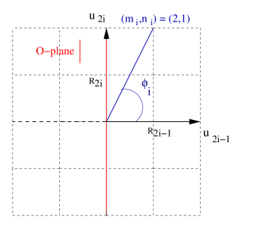
Figure 1: T-duality along the vertical axis $u_{2i}$. The $D$-brane dual to a magnetized brane forms an angle $\frac{\pi}{2}-\phi$ with respect to the vertical axis. The orientifold plane, T-dual to an $O3$-plane, sits along the vertical axis.

2.2 Moduli stabilization

From now on, we will focus our attention to the orientifold compactification $T^{6}/\mathbb{Z}_{2}$ with $\theta_{O3}=0$. Following our analysis of eqs. (2.2) and (2.3), we have seen that a single magnetized $D9$ brane stack preserves $\mathcal{N}=1$ supersymmetry in four dimensions for a restricted closed string moduli space. As we will see below, if we introduce several magnetic fluxes in the world-volume of different stacks of $D9$ branes, it will be possible to fix completely all closed string moduli but the dilaton.

As in [3], eqs. (2.2) and (2.6) can be interpreted as conditions which fix the moduli in terms of the magnetic fluxes. More specifically, we consider $K$ stacks of $N_{a}$ $D9$ branes, with $a=1,\cdots,K$. We introduce on each stack a background magnetic field with constant field strength $F^{a}$ on the corresponding world-volume and endpoint charge $q_{a}$. The magnetic fields are separately quantized, following the Dirac condition [12]

$$q_{a}F^{a}_{kl}=2\pi\cdot\frac{m^{a}_{kl}}{n^{a}_{kl}}\equiv 2\pi\cdot p^{a}_{kl}\,\,\,,\ p^{a}_{kl}\in\mathbb{Q}\,\,\,,\,\,\,a=1,\cdots,K\,.$$ (2.13)

Written in the complex coordinates (A.4), the field strength is decomposed in a purely holomorphic and mixed part.

The supersymmetry conditions for each stack ask then for a vanishing purely holomorphic field strength:

$$F_{(2,0)}=0\rightarrow\tau^{T}p^{a}_{xx}\tau-\tau^{T}{p^{a}_{xy}}-p^{a}_{yx}\tau+p^{a}_{yy}=0,\,$$ (2.14)

where the matrices $(p^{a}_{xx})_{ij}$, $(p^{a}_{xy})_{ij}$ and $(p^{a}_{yy})_{ij}$ enter in the quantized field strength (2.13) in the directions $(x^{i},x^{j})$, $(x^{i},y^{j})$ and $(y^{i},y^{j})$, respectively, where $\tau$ is the complex structure matrix. The second condition (2.6) restricts the Kähler moduli to satisfy

$$J\wedge J\wedge J-J\wedge\mathcal{F}^{a}\wedge\mathcal{F}^{a}=0\,\,\,,\ a=1,\cdots,K\,.$$ (2.15)

We have used the fact that the phases $\theta_{a}$’s of all stacks have to be the same in order for each stack to preserve the same supersymmetry: $\theta_{a}=0,\,\,\,\forall a=1,\dots,K$. Furthermore, when the condition (2.14) is fulfilled, the expression for the magnetized field strength $F$, denoted $\mathcal{F}$ in the complex basis (A.10), reduces to the matrix:

$$\mathcal{F}^{a}=\left(\begin{array}[]{cc}0&Y^{a}\\ {Y^{a}}^{\dagger}&0\\ \end{array}\right)\quad;\quad Y^{a}=\frac{1}{2}(2\pi)^{2}\alpha^{\prime}{\rm{Im}}{\tau^{-1}}^{T}\left(p_{yx}^{a}-\tau^{T}p^{a}_{xx}\right)\,.$$ (2.16)

This splits in the real and imaginary parts:

$${\rm{Re}}Y^{a} = \frac{(2\pi)^{2}\alpha^{\prime}}{2}{\rm{Im}}{\tau^{-1}}^{T}\left(p^{a}_{yx}-{\rm{Re}}\tau^{T}p^{a}_{xx}\right)\,,$$ (2.17)

$${\rm{Im}}Y^{a} = -\frac{(2\pi)^{2}\alpha^{\prime}}{2}p^{a}_{xx}\,.$$ (2.18)

Inspection of eqs. (2.14) and (2.15) shows that for each stack of magnetized $D9$ branes, we have up to three complex conditions for the moduli of the complex structure, depending on the directions in which the fluxes are switched on, whereas only one real condition can be set on the Kähler moduli. Therefore, in order to fix the Kähler moduli, we must add more stacks of branes compared to the ones needed to fix the same number of complex structure moduli and at least nine in order to fix them all.

2.3 Consistency conditions

The presence of constant internal magnetic field strength induces lower dimensional charges and tensions. In a consistent compactification, these have to be cancelled by the contribution of lower dimensional objects (branes or orientifold planes) or other kinds of fluxes (such as 3-form fluxes). In the case of a $T^{6}/\mathbb{Z}_{2}$ compactification where the supersymmetry conditions (2.2) and (2.6) are satisfied, the Dirac-Born-Infeld (DBI) and Wess-Zumino (WZ) action of magnetized $D9$ branes read:

$$V_{DBI} = -T_{9}\sum_{a=1}^{K}\,N_{a}\int_{\mathcal{M}_{10}^{a}}\sqrt{|g+\mathcal{F}^{a}|}$$

$$= -T_{9}\,\sum_{a=1}^{K}\,N_{a}\int_{\mathcal{M}_{4}}\sqrt{|g_{4}|}\int_{\mathcal{M}^{a}_{6}}{\rm Re}\,[e^{-i\theta_{a}}(iJ+\mathcal{F}^{a})^{3}]$$

$$= -T_{9}\sum_{a=1}^{K}\,N_{a}\int_{\mathcal{M}_{4}}\sqrt{|g_{4}|}\int_{\mathcal{M}^{a}_{6}}\bigg{\{}\,\mathcal{F}^{a}\wedge\mathcal{F}^{a}\wedge\mathcal{F}^{a}-J\wedge J\wedge\mathcal{F}^{a}\bigg{\}}$$

$$V_{WZ} = \mu_{9}\sum_{a=1}^{K}\,N_{a}\int_{\mathcal{M}^{a}_{10}}Ce^{\mathcal{F}^{a}}$$ (2.19)

$$= \mu_{9}\sum_{a=1}^{K}\,N_{a}\int_{\mathcal{M}^{a}_{10}}\bigg{\{}C_{4}\wedge\mathcal{F}^{a}\wedge\mathcal{F}^{a}\wedge\mathcal{F}^{a}+C_{8}\wedge\mathcal{F}^{a}\bigg{\}}$$

where $T_{9}$ and $\mu_{9}$ are the $D9$ brane tension and R-R charge, respectively, while the integral over the internal manifold $\mathcal{M}^{a}_{6}$ takes into account the winding numbers $n_{kl}^{a}$ of the different branes. The terms involving the R-R potentials $C_{10}$ and $C_{6}$ terms do not appear in the WZ action as they are projected out by the orientifold projection.

Consider now the real basis $\omega_{r}$ of $H^{2}(T^{6})$, with $r=1,\cdots,h_{2}$, in which the quantization condition (2.13) for the magnetic fluxes reads:

$$\frac{1}{2\pi}q_{a}F^{a}_{r}=\frac{m^{a}_{r}}{n^{a}_{r}}=p^{a}_{r}\,.$$ (2.20)

We now define the quantity

$$\mathcal{K}_{rst}=\int_{T^{6}}\omega_{r}\wedge\omega_{s}\wedge\omega_{t}$$ (2.21)

which is a sign, following the orientation choice given in (A.1). The 3-brane R-R charge, $q_{3,R}$, coming from the first term of the last line of (2.19), reads

$$q_{3,R}=\sum_{a=1}^{K}\,\,N_{a}\sum_{r,s,t}\,\,\mathcal{K}_{rst}m^{a}_{r}m^{a}_{s}m^{a}_{t}\,.$$ (2.22)

Since we start with a $T^{6}/\mathbb{Z}_{2}$ orientifold with $O3$ planes carrying $-16$ units of R-R charge, the R-R tadpole cancellation condition implies

$$q_{3,R}=16\,.$$ (2.23)

The second set of conditions comes from the induced 7-brane R-R charges, emerging from the second term of eqs. (2.19). For each 2-cycle $C^{(2)}_{t}$ of the torus $T^{6}$, there is a localized 7-brane charge, given by $q_{7,R}^{t}$:

$$q_{7,R}^{t}=\sum_{a=1}^{K}\,\,N_{a}\,\sum_{r,s}\,\mathcal{K}_{rst}\,n^{a}_{r}n^{a}_{s}m^{a}_{t}=:\sum_{a=1}^{K}\,N_{a}\,q^{a}_{t}\,.$$ (2.24)

In the $T^{6}/\mathbb{Z}_{2}$ compactification, 7-dimensional orientifold planes are absent and the total 7-brane tadpole contribution must thus vanish for any 2-cycle $t$:

$$q_{7,R}^{t}=0\,\,\,,\,\,\,\forall t=1,\cdots,h_{2}\,.$$ (2.25)

As a result, we will impose the R-R tadpole cancellation conditions (2.23) and (2.25): $q_{3,R}=16$ and $q_{7,R}^{t}=0$, together with the supersymmetry constraints (2.2) or equivalently (2.14), and (2.15).

Furthermore, even if magnetized antibranes may preserve the same supersymmetry as the orientifold $T^{6}/\mathbb{Z}_{2}$, satisfying a different condition than (2.15) [13], here we will consider only a setup without antibranes. In the T-dual picture of $D6$ branes at angles presented in the previous section, the $O6$ plane is located along the axis $u_{2i}$. Then, from Figure 2, the image of a brane with quantum numbers $(m_{i},n_{i})$, $i=1,2,3$, under the orientifold projection is a brane with quantum numbers $(m_{i},-n_{i})$. Moreover, an antibrane $\bar{D}6$ is obtained by a rotation by an angle $\pi$ from the corresponding $D6$ brane in an odd number of cycles $[u_{2i-1}u_{2i}]$, corresponding to a brane with winding numbers $(-m_{i},-n_{i})$. Therefore, the absence of antibranes is expressed as a condition on the winding numbers along the $u_{2i}$ axis, or equivalently on the first Chern numbers:

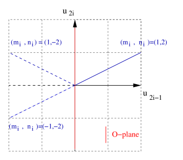
Figure 2: Example of a brane at angle with its orientifold image and antibrane. The $O$-plane is situated on the vertical axis.

$$K_{rst}m^{a}_{r}m^{a}_{s}m^{a}_{t}>0\quad\quad\forall a=1,\dots K.$$ (2.26)

The limiting case where one of the first Chern numbers $m_{i}$ vanishes, along the coordinates $u_{2i}$ corresponds to the situation where the brane is horizontal in one of the 2-cycles $[u_{2i-1}u_{2i}]$. Switching the sign of the winding number $n_{i}$ corresponds then to switch a brane into an antibrane. The condition for the absence of antibranes in this case then reads:

$$K_{rst}m^{a}_{r}m^{a}_{s}n^{a}_{t}>0\quad\quad\forall a=1,\dots K\,.$$ (2.27)

Next, a condition of positivity for the real part of $\Phi_{a}$ defined in eq. (2.5) has to be satisfied for each $a$, as it corresponds to the generalized world-volume element of each separate brane stack:

$${\rm Re}(e^{-i\theta_{a}}\Phi_{a})>0\,,\quad\forall\,a=1,\cdots,K\,,$$ (2.28)

with

$$\Phi_{a}=(iJ+\mathcal{F}^{a})\wedge(iJ+\mathcal{F}^{a})\wedge(iJ+\mathcal{F}^{a})\,.$$ (2.29)

For $\theta_{a}=0$, it reduces to the condition:

$$\mathcal{F}^{a}\wedge\mathcal{F}^{a}\wedge\mathcal{F}^{a}-J\wedge J\wedge\mathcal{F}^{a}>0\,.$$ (2.30)

Let us consider two cases which will arise in the examples of the following sections.

• When only the diagonal Kähler form elements $J_{i}=:J_{i\bar{i}}$ are non-zero and all off-diagonal fluxes vanish $F_{i\bar{j}}=0$, the positivity condition (2.30), together with the supersymmetry condition (2.15), reads:

  $$-J_{1}J_{2}J_{3}(H_{2}+H_{3})\left(1+H_{1}^{2}\right)>0,$$ (2.31)

  where we use the notation $F_{i}=F_{i\bar{i}}$ and $H_{i}=F_{i}/J_{i}$. As all Kähler moduli $J_{i}$ are volumes, they are positive and the above condition becomes

  $$H_{2}+H_{3}<0\,.$$ (2.32)

• In the last case we will consider, there are also non-diagonal fluxes, like for example $F_{1\bar{2}}$, together with a diagonal one $F_{3}$. Eq. (2.30) then reads

  $$-F_{3}|F_{1\bar{2}}|^{2}\left(1+\frac{J_{1}J_{2}}{|F_{1\bar{2}}|^{2}}\right)>0,$$ (2.33)

  implying that the diagonal component $F_{3}$ has to be negative.

Finally, we compute the intersection number $I_{ab}$ between the stacks $a$ and $b$, which gives the number of chiral fermions. As it has been shown in [6], $I_{ab}$ in the presence of a general magnetic flux can be written as

$$I_{ab} = -\frac{W_{a}W_{b}}{(2\pi)^{3}}\int_{T^{6}}c_{3}(L_{a}\otimes L_{b})$$ (2.34)

$$= W_{a}W_{b}\sum_{rst}K_{rst}\frac{(m^{a}_{r}n^{b}_{r}-m^{b}_{r}n^{a}_{r})(m^{a}_{s}n^{b}_{s}-m^{b}_{s}n^{a}_{s})(m^{a}_{t}n^{b}_{t}-m^{b}_{t}n^{a}_{t})}{n^{a}_{r}n^{a}_{s}n^{a}_{t}n^{b}_{r}n^{b}_{s}n^{b}_{t}},$$

where $W_{a/b}$ is the winding number of the stack $a/b$ around the whole $T^{6}$, $L_{a/b}$ corresponds to the $U(1)$ line bundle associated to the magnetic flux and $c_{3}(L_{a}\otimes L_{b})$ is the third Chern class. The intersection number $I_{ab}$ in (2.34) is associated to the degeneracy of the Landau levels and therefore has to be integer. An obvious solution of this requirement is to ask for the winding numbers $n^{a}_{r}$ of each stack $a$ to satisfy

$$W_{a}=n^{a}_{r}n^{a}_{s}n^{a}_{t}\,\,\,,\,\,\,\forall r,s,t\,\,{\rm with}\,\,K_{rst}\neq 0.$$ (2.35)

Since $I_{ab}$ depends only on the product of $W_{a}$ and $W_{b}$, the above restriction is valid up to a sign ambiguity. For each brane $a$, there is a unique winding number $W_{a}$ around the whole torus $T^{6}$ which is given up to a sign by the product of winding numbers of orthogonal 2-cycles. It corresponds to the geometrical picture where the fundamental cycles of the torus are six 1-cycles and the winding numbers $n_{r}$ around the fifteen different 2-cycles are not independent, but given in terms of products of winding numbers around 1-cycles. Note that in this case, the 7-brane charge $q_{t}^{a}$ defined in (2.24) reduces to $q_{t}^{a}=K_{rst}n_{r}n_{s}m_{t}$ without a sum over the indices $r,s$.

2.4 R-R Moduli

We have seen above that under strong constraints on the magnetic fluxes, it is in principle possible to find $\mathcal{N}=1$ supersymmetric vacua in four dimensions with stabilized metric moduli. In sections 4-5 and 7, we will give explicit examples where this is indeed achieved. Here, we want to address the question of the remaining moduli. In the orientifold compactification $T^{6}/\mathbb{Z}_{2}$, apart from the metric and dilaton moduli, the four dimensional spectrum contains massless 2-forms, which arise in the R-R sector. They correspond to the internal components of the R-R 4-form $C_{(4)}$ which survived the $\mathbb{Z}_{2}$-orientifold action defined in Section 2.1. They are decomposed in elements of three different cohomology classes $H^{1,1}(T^{6})$, $H^{2,0}(T^{6})$ and $H^{0,2}(T^{6})$:

$$(C_{(4)})_{\mu\nu i\bar{j}}\quad,\quad(C_{(4)})_{\mu\nu ij},\quad(C_{(4)})_{\mu\nu\bar{i}\bar{j}},\quad i,j=1,\dots,3$$ (2.36)

where the indices $\mu,\nu$ refer to four dimensional spacetime : $\mu,\nu=0,\dots,3$. The first nine 2-forms $(C_{(4)})_{\mu\nu i\bar{j}}$ are dual to pseudo-scalars in four dimensions; they actually form linear multiplets with the Kähler moduli $J_{i\bar{j}}$. When the latter are fixed in the presence of magnetized fluxes, they give rise to Stückelberg couplings that provide masses to some $U(1)$ gauge fields. This can be seen explicitly from the Wess Zumino action (2.19) in ten dimensions: Consider the gauge potential $A_{M}=(A_{\mu},A_{i})$ of a magnetized $U(1)$ with $A_{k}=-\frac{1}{2}F_{kl}u_{l}$. Its spacetime field strength $F_{(2)}=dA$ then couples to the 2-form $B_{(2)}^{i\bar{j}}=(C_{(4)})_{\mu\nu i\bar{j}}$ as:

$$\int_{\mathcal{M}_{10}}C_{4}\wedge\mathcal{F}\wedge\mathcal{F}\wedge\mathcal{F}\rightarrow q_{i\bar{j}}\int_{\mathcal{M}_{4}}B_{(2)}^{i\bar{j}}\wedge F_{(2)},$$ (2.37)

where the couplings $q_{i\bar{j}}$ are functions of the internal magnetic fluxes. As a result, some combination of the nine R-R 2-forms $(C_{(4)})_{\mu\nu i\bar{j}}$ is absorbed in the $U(1)$ gauge field which becomes massive.

The situation with the last six massless 2-forms in (2.36) is different. They are harmonic $(2,0)$ and $(0,2)$ forms on the internal torus and therefore elements of the cohomologies $H^{2,0}(T^{6})$ and $H^{0,2}(T^{6})$. By contraction with the holomorphic 3-form $\Omega$ of $T^{6}$, we can construct from $(C_{(4)})_{\mu\nu ij}$ and $(C_{(4)})_{\mu\nu\bar{i}\bar{j}}$ harmonic $(2,1)$ and $(1,2)$-forms on the torus:

$$B_{\mu\nu ij\bar{l}} \sim \Omega_{ij}^{\;\;\,\bar{k}}(C_{(4)})_{\mu\nu\bar{k}\bar{l}}$$

$$B_{\mu\nu\bar{i}\bar{j}l} \sim \bar{\Omega}_{\bar{i}\bar{j}}^{\;\;\,k}(C_{(4)})_{\mu\nu kl}\,.$$ (2.38)

To each harmonic $(2,0)$ and $(0,2)$ form, we can then associate a harmonic $(2,1)$ and $(1,2)$-form, associated to the complex structure moduli. Thus, the nine elements of the complex structure $\tau_{ij}$ correspond to six purely (anti-) holomorphic metric moduli and three (anti-) holomorphic R-R moduli. As shown in [6], the stabilization of the latter via the condition (2.2) can be understood by a potential generated through their mixing with the NS-NS moduli.

3 Closed string fluxes

As argued in section 2.2, all geometric moduli can be stabilized by turning on internal magnetic background fields. Moreover, the introduction of nine stacks of magnetized $D9$ branes can fix all complex structure and Kähler class moduli. Furthermore, the R-R moduli complexifying the Kähler class are absorbed into the longitudinal degrees of freedom of the $U(1)$ gauge fields, which become massive. The remaining unfixed moduli correspond to the (complex) dilaton-axion field.

3.1 Dilaton stabilization

A possible stabilization mechanism for the dilaton is by turning on R-R and NS-NS 3-form closed string fluxes, that for generic Calabi-Yau compactifications can fix also the complex structure [1]. As we are going to combine the two mechanisms, in this section we review briefly the main properties of 3-form fluxes.

Let $H_{(3)}$ and $F_{(3)}$ be the field strengths of the NS-NS 2-form $B_{(2)}$ and of the R-R 2-form $C_{(2)}$, respectively, $H_{(3)}=dB_{(2)}$ $F_{(3)}=dC_{(2)}$, subject as usual to the Dirac quantization condition in the compact space. In the basis $(\alpha_{a},\beta_{b})$ chosen in (A.2) of Appendix A, $H_{(3)}$ and $F_{(3)}$ can be written as

$$\frac{1}{(2\pi)^{2}\alpha^{\prime}}H_{(3)} = \sum_{a=0}^{h_{2,1}}\left(h^{a}_{1}\alpha_{a}+h^{a}_{2}\beta_{a}\right)$$

$$\frac{1}{(2\pi)^{2}\alpha^{\prime}}F_{(3)} = \sum_{a=0}^{h_{2,1}}\left(f^{a}_{1}\alpha_{a}+f^{a}_{2}\beta_{a}\right),$$ (3.1)

where $h_{1}^{a}$, $h_{2}^{a}$, $f_{1}^{a}$ and $f_{2}^{a}$ are integers. Using the complex dilaton modulus, one can then form the 3-form $G_{(3)}$

$$G_{(3)}=F_{(3)}-\phi H_{(3)}\quad,\quad\phi=C_{(0)}+ig_{s}^{-1},$$ (3.2)

where $g_{s}$ is the string coupling. The 3-form background fields preserve then a common supersymmetry with the $\mathbb{Z}_{2}$-orientifold projection of $T^{6}/\mathbb{Z}_{2}$ if the following conditions are fulfilled: $G_{(3)}$ has to be a primitive $(2,1)$ form [14]:

$$G_{(3)}\wedge J=0\quad,\quad{G_{(3)}}\in H^{2,1}.$$ (3.3)

Actually, the second of the conditions above corresponds to finding a minimum of the GVW superpotential [15]

$$W=\int_{T^{6}}G_{(3)}\wedge\Omega,$$ (3.4)

which then has to be covariantly constant with respect to all moduli, $D_{I}W=0$, or equivalently:

$$W=0\quad,\quad\partial_{\phi}W=0\quad,\quad\partial_{\tau_{ij}}W=0,$$ (3.5)

where $\phi$ is defined in (3.2). Note that all primitive $(2,1)$-forms are imaginary self dual (ISD), $\star_{6}G_{2,1}=iG_{2,1}$, where the star map $\star_{6}$ is the usual Hodge map on the torus.

Let us analyze further the supersymmetry conditions (3.5). For given flux quanta (3.1), they can be understood as conditions on the dilaton and complex structure moduli. More precisely, using the symplectic structure (A.3), the superpotential (3.4) reads

$$W=\frac{1}{(2\pi)^{2}\alpha^{\prime}}\int_{T^{6}}G_{(3)}\wedge\Omega=-(f_{1}^{0}-\phi h_{1}^{0}){\rm det}\tau+(f_{2}^{0}-\phi h_{2}^{0})+(f_{1}^{ij}-\phi h_{1}^{ij})({\rm cof}\tau)_{ij}+(f_{2}^{ij}-\phi h_{2}^{ij})\tau_{ij}.$$ (3.6)

We can now express the three supersymmetry conditions (3.5) explicitly in the form :

$$0 = -(f_{1}^{0}-\phi h_{1}^{0})det\tau+(f_{2}^{0}-\phi h_{2}^{0})+(f_{1}^{ij}-\phi h_{1}^{ij})({\rm cof}\tau)_{ij}+(f_{2}^{ij}-\phi h_{2}^{ij})\tau_{ij}$$ (3.7)

$$0 = h_{1}^{0}det\tau-h_{2}^{0}-h_{1}^{ij}({\rm cof}\tau)_{ij}-h_{2}^{ij}\tau_{ij}$$ (3.8)

$$0 = -(f_{1}^{0}-\phi h_{1}^{0})({\rm cof}\tau)_{kl}+(f_{2}^{kl}-\phi h_{2}^{kl})+(f_{1}^{ij}-\phi h_{1}^{ij})\epsilon_{ikm}\epsilon_{jln}\tau_{mn},$$ (3.9)

where ${\rm cof}\tau=({\rm det}\tau)\tau^{-1,T}$. These are eleven conditions on the complex structure, parametrized by the nine elements $\tau_{ij}$ and the (complex) dilaton field $\phi$. It is then in principle possible to fix all complex structure and dilaton moduli in terms of adequate quanta [1]. Let us now examine the primitivity condition $G_{(2,1)}\wedge J=0$. We could naively think that this can be interpreted, for given fluxes, as conditions on the Kähler moduli. However, this condition is trivially satisfied in the case of generic Calabi-Yau compactifications, because there are no harmonic $(3,2)$ forms on these manifolds. Therefore, this condition can only become partially non-trivial on Kähler moduli for compactification manifolds with more symmetries, such as the torus.

There exist however alternative possibilities to fix the metric moduli. As shown in section 2, the presence of internal magnetic fluxes leads to conditions on both the Kähler class (2.15) and complex structure moduli (2.14). For generic Calabi-Yau spaces one can fix only the former, while for toroidal compactifications it is possible to fix all metric moduli by a suitable choice of stacks of magnetized $D9$ branes. An explicit example will be shown in section 4. On the other hand, the dilaton modulus remains unfixed, but can be stabilized using 3-form closed string fluxes. In fact, for fixed complex structure, the conditions (3.7), (3.8) and (3.9) constrain exclusively the dilaton. Moreover, as the Kähler form is fixed by the presence of magnetic fields, the primitivity condition $G_{(2,1)}\wedge J=0$ restricts the possible fluxes $G_{(2,1)}$ we can switch on. Finally, the value of the string coupling we can obtain in this way is strongly constrained by the tadpole conditions. The latter can be read off from the topological coupling of the 3-form fluxes with the R-R 4-form $C_{(4)}$ potential in the effective action of the ten-dimensional type IIB supergravity:

$$S_{CS}=\frac{1}{4i(2\pi)^{7}\alpha^{\prime 4}}\int_{\mathcal{M}_{10}}\frac{C_{(4)}\wedge G_{(3)}\wedge\bar{G}_{(3)}}{{\rm Im}\phi}=-\mu_{3}\,\frac{1}{2}{1\over(2\pi)^{4}{\alpha^{\prime}}^{2}}\int_{\mathcal{M}_{10}}C_{(4)}\wedge H_{(3)}\wedge F_{(3)},$$ (3.10)

where we defined the R-R charge $\mu_{3}$ in terms of $\alpha^{\prime}$ as $\mu_{3}=(2\pi)^{-3}{\alpha^{\prime}}^{-2}$. The coupling to $C_{(4)}$ of the magnetized $D9$ branes is given in (2.19), while the coupling of the $O3$ orientifold plane reads

$$S_{O3}=\mu_{3}Q_{O3}\int_{\mathcal{M}_{4}}C_{(4)}\,,$$ (3.11)

where the charge $Q_{O3}$ of $O3$ planes has been defined in section 2.3. Therefore, the integrated Bianchi identity for the modified R-R 5-form field strength $F_{(5)}$ reads

$$-\frac{1}{2}\frac{1}{(2\pi)^{4}\alpha^{\prime 2}}\int_{T^{6}}H_{(3)}\wedge F_{(3)}+q_{3,R}+Q_{O3}=0,$$ (3.12)

where the factor $1\over 2$ comes from the fact that the volume of the orientifold $T^{6}/\mathbb{Z}_{2}$ is half the volume of the torus $T^{6}$.

It follows from the ISD condition, that the contribution to (3.12) coming from the 3-form flux is always positive :

$$N_{3}=:-\frac{1}{2}\frac{1}{(2\pi)^{4}\alpha^{\prime 2}}\int_{T^{6}}H_{(3)}\wedge F_{(3)}=\frac{1}{2g_{s}}\int_{T^{6}}H_{(3)}\wedge\star_{6}H_{(3)}>0.$$ (3.13)

The second source for 3-brane charges in (3.12) comes from the internal magnetic fluxes. As shown in section 2.3, each stack of magnetized $D9$ branes with magnetic fluxes switched on in three orthogonal directions of $T^{6}$ contributes positively to the 3-brane charge (2.22). Finally, the 3-brane tadpole could also receive contributions from ordinary $D3$ branes. All together, the tadpole condition (2.23) is now modified as

$$N_{3}+q_{3,R}+N_{D3}+Q_{O3}=0,$$ (3.14)

where $Q_{O3}=-16$. As the first three terms in the l.h.s. of equation (3.14) contribute positively, the possible values of $N_{3}$ as well of $q_{3,R}$ are bounded. This restricts strongly the possible values of the string coupling $g_{s}$. Since the tadpole condition (3.14) asks for $N_{3}$ to remain of order one, the only possibility for the string coupling to be fixed at a small value is to get a large contribution from the integral $\int_{T^{6}}H_{(3)}\wedge\star_{6}H_{(3)}$. This depends on the quanta $h_{1}^{a}$ , $h_{2}^{a}$ of (3.1) and on the Hodge star operator. The latter only depends on the complex structure [17]. It is therefore in principle possible to fix the string coupling $g_{s}$ at small value and to keep the contribution $N_{3}$ at fixed value by stabilizing the integral $\int_{T^{6}}H_{(3)}\wedge\star_{6}H_{(3)}$ at large value with the help of either internal magnetic fields or 3-form fluxes. This will be discussed in more details in section 6.

3.2 Quantized NS-NS B field

Further restrictions on fluxes arise from the quantization condition in the orientifold $T^{6}/\mathbb{Z}_{2}$, as compared to the torus. As explained in [1], the quanta of NS-NS and R-R 3-form fluxes have to be even along any 3-cycle of $T^{6}/\mathbb{Z}_{2}$. This remains valid in the presence of magnetic fluxes, as well. However, the situation changes if one introduces a non-trivial NS-NS B field in some of the 2-cycles of the torus. Consider for instance the case where the B field is switched on only in one 2-cycle, say $[x_{3}y_{3}]$: $B_{x_{3}y_{3}}=\frac{\alpha^{\prime}}{(2\pi)^{2}}b$, where $b=0$ or $1/2$. Its consequences are:

• A change in the spectrum of the open string sector [18]. The first Chern number $m^{a}_{x_{3}y_{3}}$ of the magnetic fluxes of all stacks $a=1,\cdots,K$ gets shifted to $\tilde{m}_{x_{3}y_{3}}=m_{x_{3}y_{3}}^{a}+bn_{x_{3}y_{3}}^{a}$.

  

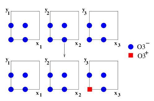
  Figure 3: $O3$ plane configuration in case of discrete torsion in the direction $[x_{3}y_{3}]$.

• A modification of the configuration of $O3$-planes. In the orientifold compactification $T^{6}/\mathbb{Z}_{2}$, there are 64 fixed points where the different $O3$ planes sit. All of them have negative tension and charge. However, for $b=1/2$, 16 of the 64 $O3$ planes become of the type $O3^{+}$, which have positive tension and charges [19]. The remaining 48 are of the usual type $O3\equiv O3^{-}$. The 3-brane tadpole condition is therefore modified. As in our conventions each $O3$ orientifold plane carries $1/4$ unit of (negative) charge, the total charge contribution of the different orientifold planes for $b=1/2$ is not anymore $-16$ but $-8$:

  $$N_{O3^{+}}-N_{O3^{-}}=\frac{1}{4}(16-48)=-8.$$ (3.15)

  The tadpole condition (3.14) is then modified to

  $$N_{3}+\tilde{q}_{3,R}+N_{D3}=8\quad,\quad\tilde{q}_{3,R}=\sum_{a=1}^{K}\,\,N_{a}\sum_{r,s,t}\,\,\mathcal{K}_{rst}\tilde{m}^{a}_{r}m^{a}_{s}m^{a}_{t}\,.$$ (3.16)

  In the modified 3-brane charge $\tilde{q}_{3,R}$ induced by the magnetic fields, it is implicitly assumed that the only shifted Chern numbers $\tilde{m}^{a}_{r}$ correspond to the 2-cycle carrying the B-field; in our example, it is $\tilde{m}^{a}_{x_{3}y_{3}}$.

• A modification of the quantization condition for the NS-NS 3-form fluxes $H_{(3)}$ [1]. Consider first a NS-NS 3-form switched on in a 3-cycle $\gamma$ of the torus $T^{6}$. If $\gamma$ crosses an odd number of orientifold planes of the type $O3^{+}$, the corresponding quanta $h_{\gamma}$ have to be odd integers, while when the crossing number is even, $h_{\gamma}$ has to be even. Let us consider now the case where $b=1/2$. As depicted in Figure 4, the sixteen $O3^{+}$ planes are located at one of the four fixed points of the third torus $[x_{3}y_{3}]$. We can easily see that the only 3-cycles of $T^{6}$, whose crossing number with the $O3^{+}$ planes is odd are the following ones:

  $$[x_{i}y_{i}x_{3}]\quad,\quad[x_{i}y_{i}y_{3}]\quad,\quad i=1,2\,\,\,.$$ (3.17)

  They correspond to 3 cycles wrapping a ‘diagonal’ 2-cycle $[x_{i}y_{i}]$ as well as one of the 1-cycles $x_{3}$ or $y_{3}$. They are located at one fixed point of the last 2-torus. As a result, the following quanta (3.1) of $H_{(3)}$ can be odd:

  $$h_{1}^{12}\quad,\quad h_{1}^{21}\quad,\quad h_{2}^{12}\quad,\quad h_{2}^{21}\,.$$ (3.18)

  

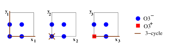
  Figure 4: Example of 3-cycle with an odd crossing number of $O3^{+}$’s. The cycle $[x_{1}y_{1}x_{3}]$ crosses a single $O3^{+}$.

4 Branes and fluxes

In this section we present the different stacks of magnetized $D9$ branes we need in order to satisfy the supersymmetry conditions (2.14), (2.15), the positivity requirements (2.26), (2.27) and (2.30), and the tadpole cancellations (2.25) and (2.23). For the shake of simplicity, our aim is to stabilize the moduli to a geometry of a factorized torus $T^{6}$ as $T^{2}\times T^{2}\times T^{2}$. This implies in particular that the off-diagonal components of the complex structure, defined in terms of the real coordinates $x^{i}$, $y^{i}$ ($i=1,2,3$) through eq. (A.4), should vanish.

The constraints on the complex structure matrix $\tau^{ij}$ are derived from eq. (2.14). We notice that, in order to have the off-diagonal components of the complex structure moduli vanishing, one needs to turn on certain off-diagonal components of magnetic fluxes on the $D9$ branes. They are characterized by rational numbers $p^{a}$’s, defined as the ratios of the quantum numbers $m$ and $n$ given in eq. (2.13). These fluxes turn out to be of the type $p^{a}_{x^{i}y^{j}}$, $p^{a}_{x^{i}x^{j}}$ and $p^{a}_{y^{i}y^{j}}$, with $i\neq j$. However, we will find out later that off-diagonal fluxes of these types have to be necessarily accompanied by certain diagonal fluxes of the type $p^{a}_{x^{i}y^{i}}$ $(i=1,2,3)$, as well. Taking these restrictions into account, the following non-zero fluxes are turned on along the branes in stack-1:

$$1.\;\;[p^{1}_{x^{1}y^{2}},\;\;p^{1}_{x^{2}y^{1}},\;\;p^{1}_{x^{1}y^{1}},\;\;p^{1}_{x^{3}y^{3}}]\neq 0,$$ (4.1)

with the remaining components of the flux being set to zero, by choosing the corresponding Chern numbers $m=0$ in eq. (2.13). The windings $n_{r}$ can be zero along some of the 2-cycles $C_{(2)}^{r}$, even if the corresponding magnetic flux vanishes. However, since the magnetized branes are $D9$’s, they have to cover the whole internal space $T^{6}/\mathbb{Z}_{2}$. This means that the effective winding number $K_{rst}n^{a}_{r}n^{a}_{s}n^{a}_{t}$ around (the 6-cycle of) $T^{6}/\mathbb{Z}_{2}$ has to be non-zero.

Similarly to (4.1), we choose for stack-2:

$$2.\;\;[p^{2}_{x^{2}y^{3}},\;\;p^{2}_{x^{3}y^{2}},\;\;p^{2}_{x^{2}y^{2}},\;\;p^{2}_{x^{1}y^{1}}]\neq 0$$ (4.2)

and for stack-3:

$$3.\;\;[p^{3}_{x^{3}y^{1}},\;\;p^{3}_{x^{1}y^{3}},\;\;p^{3}_{x^{3}y^{3}},\;\;p^{3}_{x^{2}y^{2}}]\neq 0\,.$$ (4.3)

As we will see below, the supersymmetry condition (2.14) on the stacks of branes 1-3, with fluxes turned on according to eqs. (4.1)-(4.3), imply that all off-diagonal components of $\tau^{ij}$ ($i\neq j$) are set to zero. Moreover, these conditions fix the ratios of the diagonal components $\tau^{ii}$ in terms of the ratios of $p^{a}_{x^{i}y^{j}}$ in the different brane stacks. We will also show that some magnetized branes will play a role in setting three independent combinations of the off-diagonal components of the Kähler class moduli $J_{i\bar{j}}$ to zero. In order to get similar conditions on the remaining off-diagonal components of the Kähler moduli, we introduce three more brane stacks with the following non-vanishing flux components:

$$4.\;\;[p^{4}_{x^{1}x^{2}},\;\;p^{4}_{y^{1}y^{2}},\;\;p^{4}_{x^{1}y^{1}},\;\;p^{4}_{x^{3}y^{3}}]\neq 0,$$ (4.4)

$$5.\;\;[p^{5}_{x^{2}x^{3}},\;\;p^{5}_{y^{2}y^{3}},\;\;p^{5}_{x^{2}y^{2}},\;\;p^{5}_{x^{1}y^{1}}]\neq 0,$$ (4.5)

and

$$6.\;\;[p^{6}_{x^{3}x^{1}},\;\;p^{6}_{y^{3}y^{1}},\;\;p^{6}_{x^{3}y^{3}},\;\;p^{6}_{x^{2}y^{2}}]\neq 0.$$ (4.6)

Studying various possibilities of string constructions incorporating moduli stabilization, we will also introduce in some cases six more copies of brane stacks, called stack-$1^{\prime}$ - stack-$6^{\prime}$. These branes have the same diagonal fluxes (and with brane multiplicities $N_{a^{\prime}}=N_{a}$) as their unprimed counterparts, but off-diagonal components with opposite sign:

$$1^{\prime}.\;\;[-p^{1}_{x^{1}y^{2}},\;\;-p^{1}_{x^{2}y^{1}},\;\;p^{1}_{x^{1}y^{1}},\;\;p^{1}_{x^{3}y^{3}}]\neq 0,$$ (4.7)

$$2^{\prime}.\;\;[-p^{2}_{x^{2}y^{3}},\;\;-p^{2}_{x^{3}y^{2}},\;\;p^{2}_{x^{2}y^{2}},\;\;p^{2}_{x^{1}y^{1}}]\neq 0,$$ (4.8)

$$3^{\prime}.\;\;[-p^{3}_{x^{3}y^{1}},\;\;-p^{3}_{x^{1}y^{3}},\;\;p^{3}_{x^{3}y^{3}},\;\;p^{3}_{x^{2}y^{2}}]\neq 0,$$ (4.9)

$$4^{\prime}.\;\;[-p^{4}_{x^{1}x^{2}},\;\;-p^{4}_{y^{1}y^{2}},\;\;p^{4}_{x^{1}y^{1}},\;\;p^{4}_{x^{3}y^{3}}]\neq 0,$$ (4.10)

$$5^{\prime}.\;\;[-p^{5}_{x^{2}x^{3}},\;\;-p^{5}_{y^{2}y^{3}},\;\;p^{5}_{x^{2}y^{2}},\;\;p^{5}_{x^{1}y^{1}}]\neq 0,$$ (4.11)

$$6^{\prime}.\;\;[-p^{6}_{x^{3}x^{1}},\;\;-p^{6}_{y^{3}y^{1}},\;\;p^{6}_{x^{3}y^{3}},\;\;p^{6}_{x^{2}y^{2}}]\neq 0.$$ (4.12)

The stacks 1-6 (or alternatively stacks $1^{\prime}$-$6^{\prime}$), when used with some other branes with diagonal fluxes along $[x^{i}y^{i}]$ (called stacks 7-9), give six independent conditions on the Kähler moduli $J_{i\bar{j}}$, ($i\neq j$) and force them to vanish. In our examples, we choose the stacks 7-9 having only two non-zero diagonal components of magnetic fluxes. The magnetic fields along these branes are required to satisfy the consistency conditions mentioned in section 2.3 and are sufficient to fix all diagonal components of the Kähler moduli $J$, as well. More precisely, the fluxes in stacks 7-9 read:

$$7.\;\;[p^{7}_{x^{1}y^{1}}\neq 0,\;\;p^{7}_{x^{2}y^{2}}=0,\;\;p^{7}_{x^{3}y^{3}}\neq 0],$$ (4.13)

$$8.\;\;[p^{8}_{x^{1}y^{1}}\neq 0,\;\;p^{8}_{x^{2}y^{2}}\neq 0,\;\;p^{8}_{x^{3}y^{3}}=0],$$ (4.14)

$$9.\;\;[p^{9}_{x^{1}y^{1}}=0,\;\;p^{9}_{x^{2}y^{2}}\neq 0.\;\;p^{9}_{x^{3}y^{3}}\neq 0].$$ (4.15)

Another possibility to satisfy the consistency conditions mentioned in section 2.3 is to introduce some stacks of branes with off-diagonal fluxes which do not contribute to the 3-brane tadpole:

$$10.\;\;[p^{10}_{x^{1}y^{1}}\;,\;p^{10}_{x^{3}y^{3}}\;,\;p^{10}_{x^{1}y^{3}}\;,\,p^{10}_{x^{3}y^{1}}]\neq 0,\,\,\,\,\,10^{\prime}.\;\;[p^{10^{\prime}}_{x^{1}y^{1}}\;,\;p^{10^{\prime}}_{x^{3}y^{3}}\;,\;p^{10^{\prime}}_{x^{1}x^{3}}\;,\;p^{10^{\prime}}_{y^{3}y^{1}}]\neq 0,$$ (4.16)

$$11.\;\;[p^{11}_{x^{1}y^{1}}\;,\;p^{11}_{x^{2}y^{2}}\;,\;p^{11}_{x^{1}y^{2}}\;,\;p^{11}_{x^{2}y^{1}}]\neq 0,\,\,\,\,\,11^{\prime}.\;\;[p^{11^{\prime}}_{x^{1}y^{1}}\;,\;p^{11^{\prime}}_{x^{2}y^{2}}\;,\;p^{11^{\prime}}_{x^{1}x^{2}}\;,\;p^{11^{\prime}}_{y^{2}y^{1}}]\neq 0,$$ (4.17)

$$12.\;\;[p^{12}_{x^{2}y^{2}}\;,\;p^{12}_{x^{3}y^{3}}\;,\;p^{12}_{x^{2}y^{3}}\;,\;p^{12}_{x^{3}y^{2}}]\neq 0,\,\,\,\,\,\,12^{\prime}.\;\;[p^{12^{\prime}}_{x^{2}y^{2}}\;,\;p^{12^{\prime}}_{x^{3}y^{3}}\;,\;p^{12^{\prime}}_{x^{2}x^{3}}\;,\;p^{12^{\prime}}_{y^{3}y^{2}}]\neq 0.$$ (4.18)

Of course, one has also the possibility of introducing branes with non-zero fluxes along all diagonal elements. Such branes are, however, not used in the examples we present below, for simplicity and for minimizing the 3-brane tadpole contribution.

We are now ready to examine the moduli stabilization when different combinations of branes, mentioned above, are used.

5 Explicit construction: Model-A with $q_{3,R}=6$

In this section, we analyze the conditions (2.14), (2.15), (2.30), (2.25), (2.23),(2.26) and (2.27) in more detail and present explicit examples when the twelve brane stacks 1-6, 10-12 and $10^{\prime}$-$12^{\prime}$ are used. We first discuss complex structure moduli stabilization, and next, in subsections 5.2-5.3, we show the stabilization of the Kähler class moduli, as well. These branes together contribute $q_{3,R}=6$ to the 3-brane tadpoles; tadpole cancellation will be discussed in subsection 5.5.

5.1 Stabilization of complex structure moduli

We show below that all complex structure moduli are stabilized using only the stacks of branes 1-6, with magnetic fluxes given in eqs. (4.1)-(4.6). In fact the situation remains similar to the (T-dual) case studied in [3], and we only give the final conditions following from the vanishing of the $F_{(2,0)}$ components (c.f. (2.2)), as given in (2.14).

First, the brane stacks 1-3 restrict the off-diagonal elements of the complex structure matrix by a set of six linear equations for the six variables, $\tau^{12}$, $\tau^{23}$, $\tau^{31}$, $\tau^{21}$, $\tau^{32}$, $\tau^{13}$:

$$\begin{pmatrix}0&p^{1}_{x^{2}y^{1}}&-p^{1}_{x^{3}y^{3}}\cr\cr-p^{2}_{x^{1}y^{1}}&0&p^{2}_{x^{3}y^{2}}\cr\cr p^{3}_{x^{1}y^{3}}&-p^{3}_{x^{2}y^{2}}&0\end{pmatrix}\begin{pmatrix}\tau^{12}\cr\cr\tau^{23}\cr\cr\tau^{31}\end{pmatrix}=\begin{pmatrix}-p^{1}_{x^{1}y^{1}}\tau^{13}\cr\cr-p^{2}_{x^{2}y^{2}}\tau^{21}\cr\cr-p^{3}_{x^{3}y^{3}}\tau^{32}\end{pmatrix},$$ (5.1)

$$\begin{pmatrix}-p^{1}_{x^{1}y^{2}}&0&p^{1}_{x^{3}y^{3}}\cr\cr 0&p^{3}_{x^{2}y^{2}}&-p^{3}_{x^{3}y^{1}}\cr\cr p^{2}_{x^{1}y^{1}}&-p^{2}_{x^{2}y^{3}}&0\end{pmatrix}\begin{pmatrix}\tau^{13}\cr\cr\tau^{21}\cr\cr\tau^{32}\end{pmatrix}=0.$$ (5.2)

As we will see later on, for the specific values of magnetic fluxes that we turn on along the branes, the matrix appearing in eq. (5.2) turns out to be singular and implies the equality:

$$\tau^{13}=\tau^{21}=\tau^{32}.$$ (5.3)

Moreover, the matrix appearing in the l.h.s. of eq. (5.1) is also singular, and using the result (5.3), one obtains:

$$\tau^{13}=0\quad;\quad\tau^{12}=\tau^{23}=\tau^{31}.$$ (5.4)

Finally, using the constraint (2.14) for one of the branes 4, 5 or 6, one obtains that all off-diagonal components of the complex-structure vanish:

$$\tau^{12}=\tau^{13}=\tau^{21}=\tau^{23}=\tau^{31}=\tau^{32}=0\,.$$ (5.5)

The brane stacks 1-6 also restrict the diagonal elements of the matrix $\tau$, and they satisfy the following conditions:

$$\frac{\tau^{11}}{\tau^{22}}=\frac{p^{1}_{x^{2}y^{1}}}{p^{1}_{x^{1}y^{2}}}\equiv K_{1},\;\;\;\frac{\tau^{22}}{\tau^{33}}=\frac{p^{2}_{x^{3}y^{2}}}{p^{2}_{x^{2}y^{3}}}\equiv K_{2},\;\;\;\frac{\tau^{33}}{\tau^{11}}=\frac{p^{3}_{x^{1}y^{3}}}{p^{3}_{x^{3}y^{1}}}\equiv K_{3},$$ (5.6)

and

$$\tau^{11}\tau^{22}=-\frac{p^{4}_{y^{1}y^{2}}}{p^{4}_{x^{1}x^{2}}}\equiv-K_{4},\;\;\;\tau^{22}\tau^{33}=-\frac{p^{5}_{y^{2}y^{3}}}{p^{5}_{x^{2}x^{3}}}\equiv-K_{5},\;\;\;\tau^{33}\tau^{11}=-\frac{p^{6}_{y^{3}y^{1}}}{p^{6}_{x^{3}x^{1}}}\equiv-K_{6}.$$ (5.7)

Following [3], we use $K_{1}$, $K_{3}$ and $K_{4}$ as independent parameters. Consistency between eqs. (5.6) and (5.7) then implies:

$$K_{2}={1\over K_{1}K_{3}},\;\;K_{5}={K_{3}K_{4}},\;\;K_{6}={K_{1}K_{3}K_{4}}.\;\;$$ (5.8)

Since we will look for solutions where $\tau^{ii}$ are all purely imaginary, this further imposes a positivity condition on $K_{i}$’s:

$$K_{i}>0,\;\;{\rm for}\;\;i=1,..,6.$$ (5.9)

The solutions for the diagonal elements $\tau^{ii}$ ($i=1,2,3$) are then given by:

$$\tau^{11}=i\sqrt{K_{1}K_{4}},\;\;\;\tau^{22}=i\sqrt{K_{4}\over K_{1}},\;\;\;\tau^{33}=i\sqrt{K_{1}K_{4}}K_{3}.\;\;\;$$ (5.10)

We have therefore determined the complex structure moduli completely, given by the equations (5.5) and (5.10). Using this form of the complex structure, it can also be easily verified that the stacks of branes 7-9, having fluxes only along diagonals $x^{i}y^{i}$, do not impose any further constraints on it. We go on now to the stabilization of the Kähler class moduli.

5.2 Stabilization of Kähler class moduli: constraints on fluxes

In this subsection we derive the constraints on magnetic fluxes, for the stack of branes 1-6, 10-12 and $10^{\prime}$-$12^{\prime}$, defined in section 4, in order to obtain the stabilization of the Kähler class moduli. For this purpose, we analyze the supersymmetry condition (2.15) for these stacks. As the complex structure has been stabilized to the diagonal form $\tau_{ij}=i\delta_{ij}$, the flux content given earlier in eqs. (4.1)-(4.3) can be written with the help of (2.16) as

$$1.\;\;[\mathcal{F}^{1}_{1\bar{2}}=\mathcal{F}^{1}_{2\bar{1}},\;\;\mathcal{F}^{1}_{1\bar{1}},\;\;\mathcal{F}^{1}_{3\bar{3}}]\neq 0,$$ (5.11)

$$2.\;\;[\mathcal{F}^{2}_{2\bar{3}}=\mathcal{F}^{2}_{3\bar{2}},\;\;\mathcal{F}^{2}_{2\bar{2}},\;\;\mathcal{F}^{2}_{1\bar{1}}]\neq 0,$$ (5.12)

$$3.\;\;[\mathcal{F}^{3}_{3\bar{1}}=\mathcal{F}^{3}_{1\bar{3}},\;\;\mathcal{F}^{3}_{3\bar{3}},\;\;\mathcal{F}^{3}_{2\bar{2}}]\neq 0.$$ (5.13)

In these expressions for fluxes, we have used complex coordinates, instead of the real ones used in eqs. (4.1)-(4.3), related to each other through eqs. (A.4) and (2.13). In particular, the off-diagonal components of the fluxes in eqs. (5.11) - (5.13) are purely imaginary. On the other hand, the off-diagonal fluxes in stacks 4-6 are real and they have the form:

$$4.\;\;[\mathcal{F}^{4}_{1\bar{2}}=-\mathcal{F}^{4}_{2\bar{1}},\;\;\mathcal{F}^{4}_{1\bar{1}},\;\;\mathcal{F}^{4}_{3\bar{3}}]\neq 0,$$ (5.14)

$$5.\;\;[\mathcal{F}^{5}_{2\bar{3}}=-\mathcal{F}^{5}_{3\bar{2}},\;\;\mathcal{F}^{5}_{2\bar{2}},\;\;\mathcal{F}^{5}_{1\bar{1}}]\neq 0,$$ (5.15)

$$6.\;\;[\mathcal{F}^{6}_{3\bar{1}}=-\mathcal{F}^{6}_{1\bar{3}},\;\;\mathcal{F}^{6}_{3\bar{3}},\;\;\mathcal{F}^{6}_{2\bar{2}}]\neq 0.$$ (5.16)

For the remaining branes 10-12 and $10^{\prime}$-$12^{\prime}$, the non-vanishing diagonal flux components in complex coordinates are:

$$10.\;\;[\mathcal{F}^{10}_{1\bar{1}},\;\;\mathcal{F}^{10}_{3\bar{3}},\;\;\mathcal{F}^{10}_{1\bar{3}}=\mathcal{F}^{10}_{3\bar{1}}]\neq 0,\;\;\;10^{\prime}.\;\;[\mathcal{F}^{10^{\prime}}_{1\bar{1}},\;\;\mathcal{F}^{10^{\prime}}_{3\bar{3}},\;\;\mathcal{F}^{10^{\prime}}_{1\bar{3}}=-\mathcal{F}^{10^{\prime}}_{3\bar{1}}]\neq 0,$$ (5.17)

$$11.\;\;[\mathcal{F}^{11}_{2\bar{2}},\;\;\mathcal{F}^{11}_{1\bar{1}},\;\;\mathcal{F}^{11}_{1\bar{2}}=\mathcal{F}^{11}_{2\bar{1}}]\neq 0,\;\;\;11^{\prime}.\;\;[\mathcal{F}^{11^{\prime}}_{2\bar{2}},\;\;\mathcal{F}^{11^{\prime}}_{1\bar{1}},\;\;\mathcal{F}^{11^{\prime}}_{1\bar{2}}=-\mathcal{F}^{11^{\prime}}_{2\bar{1}}]\neq 0,$$ (5.18)

$$12.\;\;[\mathcal{F}^{12}_{3\bar{3}},\;\;\mathcal{F}^{12}_{2\bar{2}},\;\;\mathcal{F}^{12}_{2\bar{3}}=\mathcal{F}^{12}_{3\bar{2}}]\neq 0,\;\;\;12^{\prime}.\;\;[\mathcal{F}^{12^{\prime}}_{3\bar{3}},\;\;\mathcal{F}^{12^{\prime}}_{2\bar{2}},\;\;\mathcal{F}^{12^{\prime}}_{2\bar{3}}=-\mathcal{F}^{12^{\prime}}_{3\bar{2}}]\neq 0.\;\;\;$$ (5.19)

We now analyze the supersymmetry condition (2.15) and find that it puts several restrictions on the fluxes that are turned on. Expressing eq. (2.15) in components, we obtain for brane-1:

$$(J\wedge J\wedge J)_{1\bar{1}2\bar{2}3\bar{3}}=J_{2\bar{2}}\mathcal{F}^{1}_{1\bar{1}}\mathcal{F}^{1}_{3\bar{3}}-J_{3\bar{3}}\mathcal{F}^{1}_{1\bar{2}}\mathcal{F}^{1}_{2\bar{1}}-(J_{1\bar{2}}+J_{2\bar{1}})\mathcal{F}^{1}_{3\bar{3}}\mathcal{F}^{1}_{2\bar{1}},$$ (5.20)

where in writing the last term we have also made use of the condition $\mathcal{F}^{1}_{2\bar{1}}=\mathcal{F}^{1}_{1\bar{2}}$ given in eq. (5.11). Similarly, we have for brane-2 and brane-3:

$$(J\wedge J\wedge J)_{1\bar{1}2\bar{2}3\bar{3}}=J_{3\bar{3}}\mathcal{F}^{2}_{2\bar{2}}\mathcal{F}^{2}_{1\bar{1}}-J_{1\bar{1}}\mathcal{F}^{2}_{2\bar{3}}\mathcal{F}^{2}_{3\bar{2}}-(J_{2\bar{3}}+J_{3\bar{2}})\mathcal{F}^{2}_{1\bar{1}}\mathcal{F}^{2}_{3\bar{2}},$$ (5.21)

$$(J\wedge J\wedge J)_{1\bar{1}2\bar{2}3\bar{3}}=J_{1\bar{1}}\mathcal{F}^{3}_{3\bar{3}}\mathcal{F}^{3}_{2\bar{2}}-J_{2\bar{2}}\mathcal{F}^{3}_{3\bar{1}}\mathcal{F}^{3}_{1\bar{3}}-(J_{3\bar{1}}+J_{1\bar{3}})\mathcal{F}^{3}_{2\bar{2}}\mathcal{F}^{3}_{1\bar{3}}.$$ (5.22)

For branes 4-6, on the other hand, we get:

$$(J\wedge J\wedge J)_{1\bar{1}2\bar{2}3\bar{3}}=J_{2\bar{2}}\mathcal{F}^{4}_{1\bar{1}}\mathcal{F}^{4}_{3\bar{3}}-J_{3\bar{3}}\mathcal{F}^{4}_{1\bar{2}}\mathcal{F}^{4}_{2\bar{1}}-(J_{1\bar{2}}-J_{2\bar{1}})\mathcal{F}^{4}_{3\bar{3}}\mathcal{F}^{4}_{2\bar{1}},$$ (5.23)

$$(J\wedge J\wedge J)_{1\bar{1}2\bar{2}3\bar{3}}=J_{3\bar{3}}\mathcal{F}^{5}_{2\bar{2}}\mathcal{F}^{5}_{1\bar{1}}-J_{1\bar{1}}\mathcal{F}^{5}_{2\bar{3}}\mathcal{F}^{5}_{3\bar{2}}-(J_{2\bar{3}}-J_{3\bar{2}})\mathcal{F}^{5}_{1\bar{1}}\mathcal{F}^{5}_{3\bar{2}},$$ (5.24)

$$(J\wedge J\wedge J)_{1\bar{1}2\bar{2}3\bar{3}}=J_{1\bar{1}}\mathcal{F}^{6}_{3\bar{3}}\mathcal{F}^{6}_{2\bar{2}}-J_{2\bar{2}}\mathcal{F}^{6}_{3\bar{1}}\mathcal{F}^{6}_{1\bar{3}}-(J_{3\bar{1}}-J_{1\bar{3}})\mathcal{F}^{6}_{2\bar{2}}\mathcal{F}^{6}_{1\bar{3}}.$$ (5.25)

Finally, the supersymmetry condition for branes 10-12 and $10^{\prime}$-$12^{\prime}$ implies:

$$(J\wedge J\wedge J)_{1\bar{1}2\bar{2}3\bar{3}}=J_{2\bar{2}}(\mathcal{F}^{10}_{3\bar{3}}\mathcal{F}^{10}_{1\bar{1}}-|\mathcal{F}^{10}_{1\bar{3}}|^{2})=J_{2\bar{2}}(\mathcal{F}^{10^{\prime}}_{3\bar{3}}\mathcal{F}^{10^{\prime}}_{1\bar{1}}-|\mathcal{F}^{10^{\prime}}_{1\bar{3}}|^{2}),$$ (5.26)

$$(J\wedge J\wedge J)_{1\bar{1}2\bar{2}3\bar{3}}=J_{3\bar{3}}(\mathcal{F}^{11}_{1\bar{1}}\mathcal{F}^{11}_{2\bar{2}}-|\mathcal{F}^{11}_{1\bar{2}}|^{2})=J_{3\bar{3}}(\mathcal{F}^{11^{\prime}}_{1\bar{1}}\mathcal{F}^{11^{\prime}}_{2\bar{2}}-|\mathcal{F}^{11^{\prime}}_{1\bar{2}}|^{2}),$$ (5.27)

$$(J\wedge J\wedge J)_{1\bar{1}2\bar{2}3\bar{3}}=J_{1\bar{1}}(\mathcal{F}^{12}_{3\bar{3}}\mathcal{F}^{12}_{2\bar{2}}-|\mathcal{F}^{12}_{2\bar{3}}|^{2})=J_{1\bar{1}}(\mathcal{F}^{12^{\prime}}_{3\bar{3}}\mathcal{F}^{12^{\prime}}_{2\bar{2}}-|\mathcal{F}^{12^{\prime}}_{2\bar{3}}|^{2}).$$ (5.28)

The fluxes along different branes are constrained in order to satisfy the supersymmetry conditions (5.20)-(5.28). As we are interested in Kähler moduli solutions with vanishing off-diagonal components $J_{i\bar{j}}=0$, and using the positivity of the volume form $J\wedge J\wedge J$, the above fluxes are restricted as:

$$J_{2\bar{2}}\mathcal{F}^{1}_{1\bar{1}}\mathcal{F}^{1}_{3\bar{3}}>J_{3\bar{3}}\mathcal{F}^{1}_{1\bar{2}}\mathcal{F}^{1}_{2\bar{1}},\;\;J_{3\bar{3}}\mathcal{F}^{2}_{2\bar{2}}\mathcal{F}^{2}_{1\bar{1}}>J_{1\bar{1}}\mathcal{F}^{2}_{2\bar{3}}\mathcal{F}^{2}_{3\bar{2}},$$ (5.29)

(5.30)

$$J_{1\bar{1}}\mathcal{F}^{3}_{3\bar{3}}\mathcal{F}^{3}_{2\bar{2}}>J_{2\bar{2}}\mathcal{F}^{3}_{3\bar{1}}\mathcal{F}^{3}_{1\bar{3}},\;\;J_{2\bar{2}}\mathcal{F}^{4}_{1\bar{1}}\mathcal{F}^{4}_{3\bar{3}}>J_{3\bar{3}}\mathcal{F}^{4}_{1\bar{2}}\mathcal{F}^{4}_{2\bar{1}},$$ (5.31)

(5.32)

$$J_{3\bar{3}}\mathcal{F}^{5}_{2\bar{2}}\mathcal{F}^{5}_{1\bar{1}}>J_{1\bar{1}}\mathcal{F}^{5}_{2\bar{3}}\mathcal{F}^{5}_{3\bar{2}},\;\;J_{1\bar{1}}\mathcal{F}^{6}_{3\bar{3}}\mathcal{F}^{6}_{2\bar{2}}>J_{2\bar{2}}\mathcal{F}^{6}_{3\bar{1}}\mathcal{F}^{6}_{1\bar{3}}.$$ (5.33)

Moreover, for branes 10-12 and $10^{\prime}$-$12^{\prime}$ one has to impose:

$$\mathcal{F}^{10}_{3\bar{3}}\mathcal{F}^{10}_{1\bar{1}}-|\mathcal{F}^{10}_{1\bar{3}}|^{2}>0,\;\;\mathcal{F}^{11}_{1\bar{1}}\mathcal{F}^{11}_{2\bar{2}}-|\mathcal{F}^{10}_{1\bar{2}}|^{2}>0,\;\;\mathcal{F}^{12}_{3\bar{3}}\mathcal{F}^{12}_{2\bar{2}}-|\mathcal{F}^{12}_{2\bar{3}}|^{2}>0,$$ (5.34)

(5.35)

$$\mathcal{F}^{10^{\prime}}_{3\bar{3}}\mathcal{F}^{10^{\prime}}_{1\bar{1}}-|\mathcal{F}^{10^{\prime}}_{1\bar{3}}|^{2}>0,\;\;\mathcal{F}^{11^{\prime}}_{1\bar{1}}\mathcal{F}^{11^{\prime}}_{2\bar{2}}-|\mathcal{F}^{11^{\prime}}_{1\bar{2}}|^{2}>0,\;\;\mathcal{F}^{12^{\prime}}_{3\bar{3}}\mathcal{F}^{12^{\prime}}_{2\bar{2}}-|\mathcal{F}^{12^{\prime}}_{2\bar{3}}|^{2}>0.$$ (5.36)

We have therefore given a set of conditions to be used for solving the supersymmetry equations (5.20)-(5.28). We postpone the discussion on their solutions for the next subsection and examine now the additional constraints imposed on fluxes from the positivity requirement (2.30). For stacks 1-6, this condition reduces to the form (2.33). The diagonal fluxes are then restricted to the domain where

$$F^{1}_{x^{3}y^{3}}<0,\;\;F^{2}_{x^{1}y^{1}}<0,\;\;F^{3}_{x^{2}y^{2}}<0,$$ (5.37)

$$F^{4}_{x^{3}y^{3}}<0,\;\;F^{5}_{x^{1}y^{1}}<0,\;\;F^{6}_{x^{2}y^{2}}<0.$$ (5.38)

When combined with conditions (5.33), this further implies that the remaining diagonal fluxes in branes 1-6 have to be negative, as well:

$$F^{1}_{x^{1}y^{1}}<0,\;\;F^{2}_{x^{2}y^{2}}<0,\;\;F^{3}_{x^{3}y^{3}}<0,$$ (5.39)

$$F^{4}_{x^{1}y^{1}}<0,\;\;F^{5}_{x^{2}y^{2}}<0,\;\;F^{6}_{x^{3}y^{3}}<0.$$ (5.40)

Finally, since the stacks 10-12 and $10^{\prime}$-$12^{\prime}$ satisfy $\mathcal{F}^{a}\wedge\mathcal{F}^{a}\wedge\mathcal{F}^{a}=0$, they do not contribute to the 3-brane charge, and the positivity conditions follow from eq. (2.32). Combined with eq. (5.36), we get that the magnetic fluxes for these branes must also be negative:

$$F^{10}_{x^{3}y^{3}}<0,\;\;\;F^{10}_{x^{1}y^{1}}<0,\;\;\;F^{10^{\prime}}_{x^{3}y^{3}}<0,\;\;\;F^{10^{\prime}}_{x^{1}y^{1}}<0,$$ (5.41)

$$F^{11}_{x^{1}y^{1}}<0,\;\;\;F^{11}_{x^{2}y^{2}}<0,\;\;\;F^{11^{\prime}}_{x^{1}y^{1}}<0,\;\;\;F^{11^{\prime}}_{x^{2}y^{2}}<0,$$ (5.42)

$$F^{12}_{x^{2}y^{2}}<0,\;\;\;F^{12}_{x^{3}y^{3}}<0,\;\;\;F^{12^{\prime}}_{x^{2}y^{2}}<0,\;\;\;F^{12^{\prime}}_{x^{3}y^{3}}<0.$$ (5.43)

5.3 Explicit solutions: fluxes and moduli

We now present an explicit solution for the fluxes along all stacks of branes satisfying the restrictions given in equations (5.8), (5.9), (5.33), (5.36) and (5.38)-(5.43). These fluxes are defined in terms of the first Chern numbers $m_{i}$’s and winding numbers $n_{i}$’s, introduced earlier in eq. (2.13), along the various 2-cycles of $T^{6}/\mathbb{Z}_{2}$. We choose for branes 1-3:

$$\begin{pmatrix}(m^{1}_{x^{1}y^{2}},n^{1}_{x^{1}y^{2}}),\;\;\;(m^{1}_{x^{2}y^{1}},n^{1}_{x^{2}y^{1}})\cr(m^{1}_{x^{1}y^{1}},n^{1}_{x^{1}y^{1}})\cr(m^{1}_{x^{2}y^{2}},n^{1}_{x^{2}y^{2}})\cr(m^{1}_{x^{3}y^{3}},n^{1}_{x^{3}y^{3}})\end{pmatrix}=\begin{pmatrix}(m^{2}_{x^{2}y^{3}},n^{2}_{x^{2}y^{3}}),\;\;\;(m^{2}_{x^{3}y^{2}},n^{2}_{x^{3}y^{2}})\cr(m^{2}_{x^{2}y^{2}},n^{2}_{x^{2}y^{2}})\cr(m^{2}_{x^{3}y^{3}},n^{2}_{x^{3}y^{3}})\cr(m^{2}_{x^{1}y^{1}},n^{2}_{x^{1}y^{1}})\end{pmatrix}=$$ (5.44)

$$\begin{pmatrix}(m^{3}_{x^{3}y^{1}},n^{3}_{x^{3}y^{1}}),\;\;\;(m^{3}_{x^{1}y^{3}},n^{3}_{x^{1}y^{3}})\cr(m^{3}_{x^{3}y^{3}},n^{3}_{x^{3}y^{3}})\cr(m^{3}_{x^{1}y^{1}},n^{3}_{x^{1}y^{1}})\cr(m^{3}_{x^{2}y^{2}},n^{3}_{x^{2}y^{2}})\end{pmatrix}=\begin{pmatrix}(-1,1),\;\;\;(1,-1)\cr(2,-1)\cr(0,-1)\cr(1,-1)\end{pmatrix},$$ (5.45)

Similarly, for branes 4-6 we choose:

$$\begin{pmatrix}(m^{4}_{x^{1}x^{2}},n^{4}_{x^{1}x^{2}}),\;\;\;(m^{4}_{y^{1}y^{2}},n^{4}_{y^{1}y^{2}})\cr(m^{4}_{x^{1}y^{1}},n^{4}_{x^{1}y^{1}})\cr(m^{4}_{x^{2}y^{2}},n^{4}_{x^{2}y^{2}})\cr(m^{4}_{x^{3}y^{3}},n^{4}_{x^{3}y^{3}})\end{pmatrix}=\begin{pmatrix}(m^{5}_{x^{2}x^{3}},n^{5}_{x^{2}x^{3}}),\;\;\;(m^{5}_{y^{2}y^{3}},n^{5}_{y^{2}y^{3}})\cr(m^{5}_{x^{2}y^{2}},n^{5}_{x^{2}y^{2}})\cr(m^{5}_{x^{3}y^{3}},n^{5}_{x^{3}y^{3}})\cr(m^{5}_{x^{1}y^{1}},n^{5}_{x^{1}y^{1}})\end{pmatrix}=$$ (5.46)

$$\begin{pmatrix}(m^{6}_{x^{3}x^{1}},n^{6}_{x^{3}x^{1}}),\;\;\;(m^{6}_{y^{3}y^{1}},n^{6}_{y^{3}y^{1}})\cr(m^{6}_{x^{3}y^{3}},n^{6}_{x^{3}y^{3}})\cr(m^{6}_{x^{1}y^{1}},n^{6}_{x^{1}y^{1}})\cr(m^{6}_{x^{2}y^{2}},n^{6}_{x^{2}y^{2}})\end{pmatrix}=\begin{pmatrix}(-1,1),\;\;\;(1,-1)\cr(2,-1)\cr(0,-1)\cr(1,-1)\end{pmatrix}.$$ (5.47)

For branes 10-12, the values of the fluxes are given by:

$$\begin{pmatrix}(m^{10}_{x^{1}y^{3}},n^{10}_{x^{1}y^{3}}),\;\;\;(m^{10}_{x^{3}y^{1}},n^{10}_{x^{3}y^{1}})\cr(m^{10}_{x^{1}y^{1}},n^{10}_{x^{1}y^{1}})\cr(m^{10}_{x^{2}y^{2}},n^{10}_{x^{2}y^{2}})\cr(m^{10}_{x^{3}y^{3}},n^{10}_{x^{3}y^{3}})\end{pmatrix}=\begin{pmatrix}(m^{11}_{x^{2}y^{1}},n^{11}_{x^{2}y^{1}}),\;\;\;(m^{11}_{x^{1}y^{2}},n^{11}_{x^{1}y^{2}})\cr(m^{11}_{x^{2}y^{2}},n^{11}_{x^{2}y^{2}})\cr(m^{11}_{x^{3}y^{3}},n^{11}_{x^{3}y^{3}})\cr(m^{11}_{x^{1}y^{1}},n^{11}_{x^{1}y^{1}})\end{pmatrix}=$$ (5.48)

$$\begin{pmatrix}(m^{12}_{x^{3}y^{2}},n^{12}_{x^{3}y^{2}}),\;\;\;(m^{12}_{x^{2}y^{3}},n^{12}_{x^{2}y^{3}})\cr(m^{12}_{x^{3}y^{3}},n^{12}_{x^{3}y^{3}})\cr(m^{12}_{x^{1}y^{1}},n^{12}_{x^{1}y^{1}})\cr(m^{12}_{x^{2}y^{2}},n^{12}_{x^{2}y^{2}})\end{pmatrix}=\begin{pmatrix}(1,-1),(-1,1)\cr(-1,1)\cr(0,1)\cr(-2,1)\end{pmatrix}\,.$$ (5.49)

Finally, the flux quanta for the stacks $10^{\prime}$-$12^{\prime}$ are the same as for the stacks 10-12 and are given by:

$$\begin{pmatrix}(m^{10^{\prime}}_{x^{1}x^{3}},n^{10^{\prime}}_{x^{1}x^{3}}),\;\;\;(m^{10^{\prime}}_{y^{1}y^{3}},n^{10^{\prime}}_{y^{1}y^{3}})\cr(m^{10^{\prime}}_{x^{1}y^{1}},n^{10^{\prime}}_{x^{1}y^{1}})\cr(m^{10^{\prime}}_{x^{2}y^{2}},n^{10^{\prime}}_{x^{2}y^{2}})\cr(m^{10^{\prime}}_{x^{3}y^{3}},n^{10^{\prime}}_{x^{3}y^{3}})\end{pmatrix}=\begin{pmatrix}(m^{11^{\prime}}_{x^{2}x^{1}},n^{11^{\prime}}_{x^{2}x^{1}}),\;\;\;(m^{11^{\prime}}_{y^{1}y^{1}},n^{11}_{y^{2}y^{1}})\cr(m^{11^{\prime}}_{x^{2}y^{2}},n^{11^{\prime}}_{x^{2}y^{2}})\cr(m^{11^{\prime}}_{x^{3}y^{3}},n^{11^{\prime}}_{x^{3}y^{3}})\cr(m^{11^{\prime}}_{x^{1}y^{1}},n^{11^{\prime}}_{x^{1}y^{1}})\end{pmatrix}=$$ (5.50)

$$\begin{pmatrix}(m^{12^{\prime}}_{x^{3}x^{2}},n^{12^{\prime}}_{x^{3}x^{2}}),\;\;\;(m^{12^{\prime}}_{y^{3}y^{2}},n^{12^{\prime}}_{y^{3}y^{2}})\cr(m^{12^{\prime}}_{x^{3}y^{3}},n^{12}_{x^{3}y^{3}})\cr(m^{12^{\prime}}_{x^{1}y^{1}},n^{12}_{x^{1}y^{1}})\cr(m^{12^{\prime}}_{x^{2}y^{2}},n^{12}_{x^{2}y^{2}})\end{pmatrix}=\begin{pmatrix}(1,-1),(-1,1)\cr(-1,1)\cr(0,1)\cr(-2,1)\end{pmatrix}\,.$$ (5.51)

Using the above values of $m$ and $n$, the non-zero fluxes defined in eq. (2.13) and used in complex structure moduli stabilization of section 5.1, for branes 1-6 read:

$$\begin{pmatrix}p^{1}_{x^{1}y^{2}}\cr p^{1}_{x^{2}y^{1}}\cr p^{1}_{x^{1}y^{1}}\cr p^{1}_{x^{3}y^{3}}\end{pmatrix}=\begin{pmatrix}p^{2}_{x^{2}y^{3}}\cr p^{2}_{x^{3}y^{2}}\cr p^{2}_{x^{2}y^{2}}\cr p^{2}_{x^{1}y^{1}}\end{pmatrix}=\begin{pmatrix}p^{3}_{x^{3}y^{1}}\cr p^{3}_{x^{1}y^{3}}\cr p^{3}_{x^{3}y^{3}}\cr p^{3}_{x^{2}y^{2}}\end{pmatrix}=\begin{pmatrix}-1\cr-1\cr-2\cr-1\end{pmatrix},$$ (5.52)

$$\begin{pmatrix}p^{4}_{x^{1}x^{2}}\cr p^{4}_{y^{1}y^{2}}\cr p^{4}_{x^{1}y^{1}}\cr p^{4}_{x^{3}y^{3}}\end{pmatrix}=\begin{pmatrix}p^{5}_{x^{2}x^{3}}\cr p^{5}_{y^{2}y^{3}}\cr p^{5}_{x^{2}y^{2}}\cr p^{5}_{x^{1}y^{1}}\end{pmatrix}=\begin{pmatrix}p^{6}_{x^{3}x^{1}}\cr p^{6}_{y^{3}y^{1}}\cr p^{6}_{x^{3}y^{3}}\cr p^{6}_{x^{2}y^{2}}\end{pmatrix}=\begin{pmatrix}-1\cr-1\cr-2\cr-1\end{pmatrix}.$$ (5.53)

Similarly, for branes 10-12 and $10^{\prime}$-$12^{\prime}$, the non-zero fluxes are given by:

$$\begin{pmatrix}p^{10}_{x^{1}y^{3}}\cr p^{10}_{x^{3}y^{1}}\cr p^{10}_{x^{1}y^{1}}\cr p^{10}_{x^{3}y^{3}}\end{pmatrix}=\begin{pmatrix}p^{11}_{x^{1}y^{2}}\cr p^{11}_{x^{2}y^{1}}\cr p^{11}_{x^{2}y^{2}}\cr p^{11}_{x^{1}y^{1}}\end{pmatrix}=\begin{pmatrix}p^{12}_{x^{2}y^{3}}\cr p^{12}_{x^{3}y^{2}}\cr p^{12}_{x^{3}y^{3}}\cr p^{12}_{x^{2}y^{2}}\end{pmatrix}=\begin{pmatrix}p^{10^{\prime}}_{x^{1}x^{3}}\cr p^{10^{\prime}}_{y^{1}y^{3}}\cr p^{10^{\prime}}_{x^{1}y^{1}}\cr p^{10^{\prime}}_{x^{3}y^{3}}\end{pmatrix}=\begin{pmatrix}p^{11^{\prime}}_{x^{1}x^{2}}\cr p^{11^{\prime}}_{y^{1}y^{2}}\cr p^{11^{\prime}}_{x^{2}y^{2}}\cr p^{11^{\prime}}_{x^{1}y^{1}}\end{pmatrix}=\begin{pmatrix}p^{12^{\prime}}_{x^{2}x^{3}}\cr p^{12^{\prime}}_{y^{2}y^{3}}\cr p^{12^{\prime}}_{x^{3}y^{3}}\cr p^{12^{\prime}}_{x^{2}y^{2}}\end{pmatrix}=\begin{pmatrix}-1\cr-1\cr-1\cr-2\end{pmatrix}.$$ (5.54)

One can now verify that the above magnetic fluxes (5.52)-(5.54) satisfy the conditions (5.8) and the parameters $K_{i}$ defined in eqs. (5.6) and (5.7) read:

$$K_{1}=\;K_{2}=\;K_{3}=\;K_{4}=\;K_{5}=\;K_{6}=1,\;\;$$ (5.55)

which obviously solve both eqs. (5.8) and (5.9). Moreover, the diagonal components of the complex structure moduli are fixed using eq. (5.10) to:

$$\tau^{11}=\tau^{22}=\tau^{33}=i.$$ (5.56)

Since all diagonal components of the fluxes (5.52)-(5.54) are negative, they also obviously satisfy the conditions (5.38)-(5.43). The conditions (5.33) and (5.36) are also satisfied, as will be shown in the following subsection 5.4.

We have therefore shown that the explicit choice for the fluxes presented in eqs. (5.52)-(5.54) satisfy the consistency requirements imposed earlier. Obviously, this choice is not unique. For instance, it is possible to modify them in a way that the products appearing in the supersymmetry conditions (5.20)-(5.28) involving also the Kähler class moduli remain invariant. Before ending this section, we also give the matrices entering in eqs. (5.1) and (5.2), for the values of fluxes (5.52)-(5.54). The $3\times 3$ matrix appearing in the l.h.s. of eq. (5.1) reads:

$$\begin{pmatrix}0&-1&1\cr\cr 1&0&-1\cr\cr-1&1&0\end{pmatrix},$$ (5.57)

while the matrix appearing in eq. (5.2)

$$\begin{pmatrix}1&0&-1\cr\cr 0&-1&1\cr\cr-1&1&0\end{pmatrix}$$ (5.58)

is singular and implies the relation (5.3): $\tau^{21}=\tau^{32}=\tau^{13}$. Using this equality in the r.h.s. of eq. (5.1) with the result (5.57), one finds: $\tau^{12}=\tau^{23}=\tau^{31}$ and $\tau^{21}=\tau^{32}=\tau^{13}=0$. Finally, using brane 4 (or brane 5-6) one obtains the result (5.5) that all off-diagonal components of the complex structure $\tau^{ij}$ are zero.

We will now obtain the values of the Kähler class moduli by solving the supersymmetry conditions. We will show that all off-diagonal components vanish, while the diagonal ones (in real coordinates) are $J_{x^{i}y^{i}}=(2\pi)^{2}\alpha^{\prime}$ (for $i=1,2,3$), defining a meaningful solution of the supersymmetry conditions (5.20)-(5.28).

5.4 Solving the supersymmetry conditions to fix the Kähler form

Here, we analyze the supersymmetry conditions (5.20)-(5.28), which consist of nine independent non-linear equations for nine variables. The reason is that the three equations in the r.h.s. of (5.26)-(5.28), related to the stacks 10-$10^{\prime}$, 11-$11^{\prime}$ and $12$-$12^{\prime}$, are trivially satisfied because of our choice of fluxes. Even if the system could in principle be solved exactly, we only present here the solution where the off-diagonal components of the Kähler form vanish, $J_{i\bar{j}}=0$ for $i\neq j$. This solution is consistent with eqs. (5.26)-(5.28), arising from the brane stacks 10-12 and $10^{\prime}$-$12^{\prime}$ with the choice of fluxes given in (5.54), for a restricted Kähler class moduli space where

$$J_{1\bar{1}}=J_{2\bar{2}}=J_{3\bar{3}}.$$ (5.59)

Moreover, the brane stacks 1-6 restrict further the Kähler moduli to

$$J_{2\bar{2}}\mathcal{F}^{1}_{1\bar{1}}\mathcal{F}^{1}_{3\bar{3}}-J_{3\bar{3}}\mathcal{F}^{1}_{1\bar{2}}\mathcal{F}^{1}_{2\bar{1}}=J_{3\bar{3}}\mathcal{F}^{2}_{2\bar{2}}\mathcal{F}^{2}_{1\bar{1}}-J_{1\bar{1}}\mathcal{F}^{2}_{2\bar{3}}\mathcal{F}^{2}_{3\bar{2}}=J_{1\bar{1}}\mathcal{F}^{3}_{3\bar{3}}\mathcal{F}^{3}_{2\bar{2}}-J_{2\bar{2}}\mathcal{F}^{3}_{3\bar{1}}\mathcal{F}^{3}_{1\bar{3}}=$$ (5.60)

(5.61)

$$J_{2\bar{2}}\mathcal{F}^{4}_{1\bar{1}}\mathcal{F}^{4}_{3\bar{3}}-J_{3\bar{3}}\mathcal{F}^{4}_{1\bar{2}}\mathcal{F}^{4}_{2\bar{1}}=J_{3\bar{3}}\mathcal{F}^{5}_{2\bar{2}}\mathcal{F}^{5}_{1\bar{1}}-J_{1\bar{1}}\mathcal{F}^{5}_{2\bar{3}}\mathcal{F}^{5}_{3\bar{2}}=J_{1\bar{1}}\mathcal{F}^{6}_{3\bar{3}}\mathcal{F}^{6}_{2\bar{2}}-J_{2\bar{2}}\mathcal{F}^{6}_{3\bar{1}}\mathcal{F}^{6}_{1\bar{3}}=$$ (5.62)

(5.63)

$$J_{2\bar{2}}(\mathcal{F}^{10}_{3\bar{3}}\mathcal{F}^{10}_{1\bar{1}}-|\mathcal{F}^{10}_{1\bar{3}}|^{2})=J_{3\bar{3}}(\mathcal{F}^{11}_{1\bar{1}}\mathcal{F}^{11}_{2\bar{2}}-|\mathcal{F}^{11}_{1\bar{2}}|^{2})=J_{1\bar{1}}(\mathcal{F}^{12}_{2\bar{2}}\mathcal{F}^{12}_{3\bar{3}}-|\mathcal{F}^{12}_{2\bar{3}}|^{2})=$$ (5.64)

(5.65)

$$J_{2\bar{2}}(\mathcal{F}^{10^{\prime}}_{3\bar{3}}\mathcal{F}^{10^{\prime}}_{1\bar{1}}-|\mathcal{F}^{10^{\prime}}_{1\bar{3}}|^{2})=J_{3\bar{3}}(\mathcal{F}^{11^{\prime}}_{1\bar{1}}\mathcal{F}^{11^{\prime}}_{2\bar{2}}-|\mathcal{F}^{11^{\prime}}_{1\bar{2}}|^{2})=J_{1\bar{1}}(\mathcal{F}^{12^{\prime}}_{2\bar{2}}\mathcal{F}^{12^{\prime}}_{3\bar{3}}-|\mathcal{F}^{12^{\prime}}_{2\bar{3}}|^{2}).$$ (5.66)

Using the choice of fluxes (5.52) - (5.54), we then get a solution for the diagonal Kähler moduli

$$J_{1\bar{1}}=J_{2\bar{2}}=J_{3\bar{3}}=\frac{(2\pi)^{2}\alpha^{\prime}}{2},$$ (5.67)

or in terms of real coordinates:

$$J_{x^{1}y^{1}}=J_{x^{2}y^{2}}=J_{x^{3}y^{3}}=(2\pi)^{2}\alpha^{\prime}\,.$$ (5.68)

To show that the conditions (5.33) and (5.36) are satisfied, we rewrite the fluxes in the complex coordinates (A.10), using (2.16) and eqs. (5.52)-(5.54):

$$\mathcal{F}^{1}_{1\bar{2}}=\mathcal{F}^{1}_{2\bar{1}}=\mathcal{F}^{2}_{2\bar{3}}=\mathcal{F}^{2}_{3\bar{2}}=\mathcal{F}^{3}_{3\bar{1}}=\mathcal{F}^{3}_{1\bar{3}}=-{1\over 2}4\pi^{2}\alpha^{\prime},$$ (5.69)

(5.70)

$$\mathcal{F}^{4}_{1\bar{2}}=-\mathcal{F}^{4}_{2\bar{1}}=\mathcal{F}^{5}_{2\bar{3}}=-\mathcal{F}^{5}_{3\bar{2}}=\mathcal{F}^{6}_{3\bar{1}}=-\mathcal{F}^{6}_{1\bar{3}}=2\pi^{2}i\alpha^{\prime}\,,$$ (5.71)

and

$$\mathcal{F}^{1}_{1\bar{1}}=\mathcal{F}^{2}_{2\bar{2}}=\mathcal{F}^{3}_{3\bar{3}}=\mathcal{F}^{4}_{1\bar{1}}=\mathcal{F}^{5}_{2\bar{2}}=\mathcal{F}^{6}_{3\bar{3}}=-4\pi^{2}\alpha^{\prime}$$ (5.72)

$$\mathcal{F}^{1}_{3\bar{3}}=\mathcal{F}^{2}_{1\bar{1}}=\mathcal{F}^{3}_{2\bar{2}}=\mathcal{F}^{4}_{3\bar{3}}=\mathcal{F}^{5}_{1\bar{1}}=\mathcal{F}^{6}_{2\bar{2}}=-2\pi^{2}\alpha^{\prime}\,.$$ (5.73)

It is then easy to see that the conditions (5.33) are satisfied, using the result $J_{1\bar{1}}=J_{2\bar{2}}=J_{3\bar{3}}$. Similarly, the conditions (5.36) are satisfied using the following expressions for the magnetic fluxes along the branes 10-12 in complex coordinates:

$$2\mathcal{F}^{10}_{1\bar{1}}=\mathcal{F}^{10}_{3\bar{3}}=2\mathcal{F}^{11}_{2\bar{2}}=\mathcal{F}^{11}_{1\bar{1}}=2\mathcal{F}^{12}_{3\bar{3}}=\mathcal{F}^{12}_{2\bar{2}}=-4\pi^{2}\alpha^{\prime},$$ (5.74)

(5.75)

$$2\mathcal{F}^{10}_{1\bar{3}}=2\mathcal{F}^{10}_{3\bar{1}}=2\mathcal{F}^{11}_{2\bar{1}}=\mathcal{F}^{11}_{1\bar{2}}=2\mathcal{F}^{12}_{3\bar{2}}=\mathcal{F}^{12}_{2\bar{3}}=-4\pi^{2}\alpha^{\prime},$$ (5.76)

and for the branes $10^{\prime}$-$12^{\prime}$:

$$2\mathcal{F}^{10^{\prime}}_{1\bar{1}}=\mathcal{F}^{10^{\prime}}_{3\bar{3}}=2\mathcal{F}^{11^{\prime}}_{2\bar{2}}=\mathcal{F}^{11^{\prime}}_{1\bar{1}}=2\mathcal{F}^{12^{\prime}}_{3\bar{3}}=\mathcal{F}^{12^{\prime}}_{2\bar{2}}=-4\pi^{2}\alpha^{\prime},$$ (5.77)

(5.78)

$$2\mathcal{F}^{10^{\prime}}_{1\bar{3}}=2\mathcal{F}^{10^{\prime}}_{3\bar{1}}=2\mathcal{F}^{11^{\prime}}_{2\bar{1}}=\mathcal{F}^{11^{\prime}}_{1\bar{2}}=2\mathcal{F}^{12^{\prime}}_{3\bar{2}}=\mathcal{F}^{12^{\prime}}_{2\bar{3}}=4\pi^{2}i\alpha^{\prime}.$$ (5.79)

5.5 Tadpole cancellations

We now analyze the tadpole cancellation conditions, written in equations (2.25), (2.23) and (3.14) for model-A, specified by the quantum numbers $(m,n)$ of eqs. (5.45)-(5.51). We start with the analysis of the 7-brane R-R tadpoles (2.25). The expressions for the tadpole contributions $q^{a}_{t}$ from the $a$-th brane, localized at the 2-cycle $C_{t}^{(2)}$, are given in eq. (2.24). For example, brane-1 has a potential contribution in the following 2-cycles:

$$q^{1}_{[x^{1}y^{2}]}=-n^{1}_{x^{3}y^{3}}n^{1}_{x^{2}y^{1}}m^{1}_{x^{1}y^{2}}\,\,\,,\,\,\,q^{1}_{[x^{2}y^{1}]}=-n^{1}_{x^{3}y^{3}}n^{1}_{x^{1}y^{2}}m^{1}_{x^{2}y^{1}}\,\,\,,$$ (5.80)

$$q^{1}_{[x^{1}y^{1}]}=n^{1}_{x^{2}y^{2}}n^{1}_{x^{3}y^{3}}m^{1}_{x^{1}y^{1}}\,\,,\,\,q^{1}_{[x^{2}y^{2}]}=n^{1}_{x^{1}y^{1}}n^{1}_{x^{3}y^{3}}m^{1}_{x^{2}y^{2}}\,\,,\,\,q^{1}_{[x^{3}y^{3}]}=n^{1}_{x^{1}y^{1}}n^{1}_{x^{2}y^{2}}m^{1}_{x^{3}y^{3}}.$$ (5.81)

By inserting the values of $m$’s and $n$’s from eq. (5.45), we obtain for brane-1:

$$q^{1}_{[x^{1}y^{2}]}=1,\;\;q^{1}_{[x^{2}y^{1}]}=1,\;\;q^{1}_{[x^{1}y^{1}]}=2,\;\;q^{1}_{[x^{2}y^{2}]}=0,\;\;q^{1}_{[x^{3}y^{3}]}=1\,,$$ (5.82)

and similarly for brane-2:

$$q^{2}_{[x^{2}y^{3}]}=1,\;\;q^{2}_{[x^{3}y^{2}]}=1\;\;q^{2}_{[x^{2}y^{2}]}=2,\;\;q^{2}_{[x^{3}y^{3}]}=0,\;\;q^{2}_{[x^{1}y^{1}]}=1\,,$$ (5.83)

and brane-3:

$$q^{3}_{[x^{3}y^{1}]}=1,\;\;q^{3}_{[x^{1}y^{3}]}=1\;\;q^{3}_{[x^{3}y^{3}]}=2,\;\;q^{3}_{[x^{1}y^{1}]}=0,\;\;q^{3}_{[x^{2}y^{2}]}=1\,.$$ (5.84)

The computation is similar for brane-4 to brane-6 with fluxes given in eqs. (5.47). The result for the 7-brane charges is:

$$q^{4}_{[x^{1}x^{2}]}=1,\;\;q^{4}_{[y^{1}y^{2}]}=1,\;\;q^{4}_{[x^{1}y^{1}]}=2,\;\;q^{4}_{[x^{2}y^{2}]}=0,\;\;q^{4}_{[x^{3}y^{3}]}=1\,,$$ (5.85)

$$q^{5}_{[x^{2}x^{3}]}=1,\;\;q^{5}_{[y^{2}y^{3}]}=1.\;\;q^{5}_{[x^{2}y^{2}]}=2,\;\;q^{5}_{[x^{3}y^{3}]}=0,\;\;q^{5}_{[x^{1}y^{1}]}=1\,,$$ (5.86)

$$q^{6}_{[x^{3}x^{1}]}=1,\;\;q^{6}_{[y^{3}y^{1}]}=1,\;\;q^{6}_{[x^{3}y^{3}]}=2,\;\;q^{6}_{[x^{1}y^{1}]}=0,\;\;q^{6}_{[x^{2}y^{2}]}=1\,.$$ (5.87)

Assuming that each stack contains only one brane $N_{a}=1$ $\forall a$, and adding the above contributions to the 7-brane tadpoles from branes 1-6, we obtain a non-vanishing result for the diagonal 2-cycles $[x^{1}y^{1}]$, $[x^{2}y^{2}]$, $[x^{3}y^{3}]$:

$$\sum_{a=1}^{6}\,N_{a}\,q^{a}_{t}=6\quad,\quad t=[x^{1}y^{1}],[x^{2}y^{2}],[x^{3}y^{3}]\,.$$ (5.88)

On the other hand, for each of the twelve off-diagonal 2-cycles: $[x^{i}y^{j}]$,$[x^{i}x^{j}]$,$[y^{i}y^{j}]$ for $i\neq j$ we have:

$$\sum_{a=1}^{6}\,N_{a}\,q^{a}_{t}=1\quad,\quad t=[x^{i}y^{j}]\,,\,[x^{i}x^{j}]\,,\,[y^{i}y^{j}]\,,\;i\neq j.$$ (5.89)

The 7-brane tadpole contributions for the branes 10-12 with fluxes and quantum numbers $(m,n)$ given in eq. (5.49) are also non-vanishing and read:

$$q^{10}_{[x^{1}y^{1}]}=n^{10}_{x^{2}y^{2}}n^{10}_{x^{3}y^{3}}m^{10}_{x^{1}y^{1}}=-1\,\,\,,\,\,\,q^{10}_{[x^{3}y^{3}]}=n^{10}_{x^{1}y^{1}}n^{10}_{x^{2}y^{2}}m^{10}_{x^{3}y^{3}}=-2\,,$$ (5.90)

$$q^{10}_{[x^{1}y^{3}]}=-n^{10}_{x^{2}y^{2}}n^{10}_{x^{3}y^{1}}m^{10}_{x^{1}y^{3}}=-1\,\,\,,\,\,\,q^{10}_{[x^{3}y^{1}]}=-n^{10}_{x^{2}y^{2}}n^{10}_{x^{1}y^{3}}m^{10}_{x^{3}y^{1}}=-1\,,$$ (5.91)

$$q^{{11}}_{[x^{2}y^{2}]}=n^{11}_{x^{3}y^{3}}n^{11}_{x^{1}y^{1}}m^{11}_{x^{2}y^{2}}=-1\,\,\,,\,\,\,q^{{11}}_{[x^{1}y^{1}]}=n^{11}_{x^{2}y^{2}}n^{11}_{x^{3}y^{3}}m^{11}_{x^{1}y^{1}}=-2,$$ (5.92)

$$q^{{11}}_{[x^{2}y^{1}]}=n^{11}_{x^{3}y^{3}}n^{11}_{x^{1}y^{2}}m^{11}_{x^{2}y^{1}}=-1\,\,\,,\,\,\,q^{{11}}_{[x^{1}y^{2}]}=n^{11}_{x^{2}y^{2}}n^{11}_{x^{2}y^{1}}m^{11}_{x^{1}y^{2}}=-1,$$ (5.93)

$$q^{12}_{[x^{3}y^{3}]}=n^{12}_{x^{1}y^{1}}n^{12}_{x^{2}y^{2}}m^{12}_{x^{3}y^{3}}=-1\,\,\,,\,\,\,q^{12}_{[x^{2}y^{2}]}=n^{12}_{x^{3}y^{3}}n^{12}_{x^{1}y^{1}}m^{12}_{x^{2}y^{2}}=-2,$$ (5.94)

$$q^{12}_{[x^{3}y^{2}]}=-n^{12}_{x^{1}y^{1}}n^{12}_{x^{2}y^{3}}m^{12}_{x^{3}y^{2}}=-1\,\,\,,\,\,\,q^{12}_{[x^{2}y^{3}]}=-n^{12}_{x^{1}y^{1}}n^{12}_{x^{3}y^{2}}m^{12}_{x^{2}y^{3}}=-1.$$ (5.95)

Similarly, the contributions of the branes $10^{\prime}$-$12^{\prime}$ read:

$$q^{10^{\prime}}_{[x^{1}y^{1}]}=-1\,\,\,,\,\,\,q^{10^{\prime}}_{[x^{3}y^{3}]}=-2\,q^{10^{\prime}}_{[x^{1}x^{3}]}=-1\,\,\,,\,\,\,q^{10^{\prime}}_{[y^{1}y^{3}]}=-1\,,$$ (5.96)

$$q^{{11^{\prime}}}_{[x^{2}y^{2}]}=-1\,\,\,,\,\,\,q^{{11^{\prime}}}_{[x^{1}y^{1}]}=-2,\,q^{{11^{\prime}}}_{[x^{1}x^{2}]}=-1\,\,\,,\,\,\,q^{{11^{\prime}}}_{[y^{1}y^{2}]}=-1\,,$$ (5.97)

$$q^{12^{\prime}}_{[x^{3}y^{3}]}=-1\,\,\,,\,\,\,q^{12^{\prime}}_{[x^{2}y^{2}]}=-2,\,q^{12^{\prime}}_{[x^{2}x^{3}]}=-1\,\,\,,\,\,\,q^{12^{\prime}}_{[y^{2}y^{3}]}=-1.$$ (5.98)

Adding the results of eqs. (5.91)-(5.98), we obtain the (non-vanishing) contributions of branes 10-12 and $10^{\prime}$-$12^{\prime}$ to the 7-brane tadpoles:

$$q_{7,R}^{t}=\sum_{a=10}^{12}\,N_{a}\,q^{a}_{t}+\sum_{a=10^{\prime}}^{12^{\prime}}\,N_{a}\,q^{a}_{t}=-6\quad,\quad t=[x^{1}y^{1}],[x^{2}y^{2}],[x^{3}y^{3}]\,.$$ (5.99)

For off-diagonal 2-cycles one now has:

$$\sum_{a=10}^{12}\,N_{a}\,q^{a}_{t}+\sum_{a=10^{\prime}}^{12^{\prime}}\,N_{a}\,q^{a}_{t}=-1\quad,\quad t=[x^{i}y^{j}]\,,\,[x^{i}x^{j}]\,,\,[y^{i}y^{j}]\,,\;i\neq j.$$ (5.100)

From eqs. (5.88), (5.89) and (5.99), (5.100), we conclude that the total 7-brane R-R tadpoles vanish for all 2-cycles, when the contributions of all the branes are added.

Let us now discuss the 3-brane tadpole cancellation. It can be directly verified, using (2.23), the brane multiplicities $N_{a}=1$ for each of the twelve stacks, and the quantum numbers $m$ specified in eqs. (5.45)-(5.51) that each of the branes 1-6 contributes $q^{a}_{3,R}=1$ ($a=1,..,6$) to the 3-brane tadpole, whereas for branes 10-12 and $10^{\prime}$-$12^{\prime}$ one obtains a vanishing contribution $q^{a}_{3,R}=0$ ($a=10$-$12$, $10^{\prime}$-$12^{\prime}$). The total 3-brane tadpole contribution is therefore equal to $\sum_{a=1}^{12}q^{a}_{3,R}=6$. One possibility to cancel the 3-brane tadpole, namely to satisfy eq. (2.23), is to either take multiple copies of various branes 1-6, or/and add ordinary $D3$ branes to the system. On the other hand, one can also cancel the 3-brane tadpoles by turning on closed string 3-form fluxes, as discussed in section 3. In this way, one also has the advantage that the remaining closed string moduli, corresponding to the axion and dilaton, can be stabilized as well, specifying the string coupling uniquely.

5.6 Stabilization of the axion-dilaton moduli

As shown above, the model presented in section 5.3 is a consistent supersymmetric four dimensional perturbative vacuum with all closed string moduli but the dilaton fixed. In particular, the metric moduli, represented by the complex structure and the Kähler class are stabilized at the values

$$J_{i\bar{j}}=\frac{4\pi^{2}\alpha^{\prime}}{2}\delta_{i\bar{j}}\quad,\quad\tau^{ij}=i\delta^{ij}.$$ (5.101)

We want to address now the question of the dilaton stabilization [1] by turning on R-R and NS-NS 3-form fluxes, as explained in the section 3. Consider the case where we switch on the following quanta

$$h_{1}^{12}\quad,\quad h_{1}^{21}\quad,\quad h_{2}^{12}\quad,\quad h_{2}^{21}\,;$$ (5.102)

$$f_{1}^{12}\quad,\quad f_{1}^{21}\quad,\quad f_{2}^{12}\quad,\quad f_{2}^{21}\,.$$ (5.103)

Since the complex structure has been fixed to the purely imaginary diagonal form (5.101), the supersymmetry conditions (3.7) and (3.8) are trivially satisfied whereas eq. (3.9) fixes the dilaton in terms of the complex structure element $\tau_{33}=i$:

$$f_{2}^{12}-\phi h_{2}^{12}=\tau_{33}(f_{1}^{21}-\phi h_{1}^{21})\quad,\quad f_{2}^{21}-\phi h_{2}^{21}=\tau_{33}(f_{1}^{12}-\phi h_{1}^{12}).$$ (5.104)

The two equations can not be independent and give rise to a constraint on the allowed fluxes. Actually, these conditions are equivalent to the requirement that the $G_{(3)}$ flux must be of the type $(2,1)$. Indeed, in the complex coordinates (A.4), the only non-vanishing components of $G_{(2,1)}$ are $G_{1\bar{1}\bar{3}}$ and $G_{2\bar{2}\bar{3}}$ :

$$-2iG_{(2,1)}=(f_{1}^{21}-\phi h_{1}^{21})dz_{1}\wedge d\bar{z}_{\bar{1}}\wedge dz_{3}-(f_{1}^{12}-\phi h_{1}^{12})dz_{2}\wedge d\bar{z}_{\bar{2}}\wedge dz_{3}.$$ (5.105)

Furthermore, for the values (5.101) of the Kähler form , the primitivity condition $G_{(3)}\wedge J=0$ restricts further the fluxes to

$$(f_{1}^{12}-\phi h_{1}^{12})J_{1\bar{1}}-(f_{1}^{21}-\phi h_{1}^{21})J_{2\bar{2}}=0,\quad{\rm or\,\,equivalently}\quad(f_{1}^{12}-\phi h_{1}^{12})=(f_{1}^{21}-\phi h_{1}^{21}).$$ (5.106)

A quick computation shows that under the restriction on the fluxes coming from eqs. (5.104) and from the primitivity condition (5.106), the string coupling is given by:

$$\frac{1}{g_{s}}={\rm Im}\tau_{33}\frac{f_{2}^{21}h_{1}^{12}-f_{1}^{12}h_{2}^{21}}{(h_{1}^{12}{\rm Im}\tau_{33})^{2}+(h_{2}^{21})^{2}},$$ (5.107)

if we assume that the complex structure modulus $\tau_{33}$ has no real part, as we found in model-A. However, we keep track of the dependence of $g_{s}$ on the complex structure in order to examine (in the next section) the possible stabilization of the string coupling at small values.

To simplify the discussion, let us further reduce the number of flux components to the case where only four of them are different than zero:

$$f_{1}^{12},\;\;f_{1}^{21},\;\;h_{2}^{12},\;\;h_{2}^{21}\neq 0.$$ (5.108)

Notice that this restriction is only possible in the absence of a B-field, as explained in section 3.2. Indeed, in the presence of a $B$-field $(b=1/2)$, the flux components $h_{1}^{12}$ and $h_{1}^{21}$ have to be odd and can therefore not be set to zero. With the reduced number of non-vanishing elements (5.108), the string coupling (5.107) is then fixed to the value

$$\frac{1}{g_{s}}=-{\rm Im}\tau_{33}\frac{f_{1}^{12}}{h_{2}^{21}},$$ (5.109)

whereas the flux restrictions (5.104) and (5.106) lead to:

$$f_{1}^{12}=f_{1}^{21}\quad,\quad h_{2}^{21}=h_{2}^{12}.$$ (5.110)

In order to compute the value of the dilaton, we first have to analyze the 3-form contribution to the 3-brane tadpole (3.13). From the symplectic structure (A.3) and the restriction (5.110), the 3-form fluxes (5.108) induce a 3-brane charge

$$N_{3}=-\frac{1}{2}(h_{2}^{12}f_{1}^{12}+h_{2}^{12}f_{1}^{12})=-h_{2}^{12}f_{1}^{12},$$ (5.111)

and using the results of section 5.5, the tadpole condition (3.14) reads:

$$-h_{2}^{12}f_{1}^{12}+N_{D3}=10.$$ (5.112)

As the flux quanta (5.108) have to be even in the absence of a B-field, the minimal value we can get for the string coupling is given by $f_{1}^{12}=-4$ and $h_{2}^{12}=2$, which (for $\tau_{33}=i$) corresponds to $g_{s}=1/2$.

In fact, a smaller value of $g_{s}$ can be obtained in the presence of a non-trivial NS-NS $B$ field. Consider for instance the case where a $B_{x_{3}y_{3}}\neq 0$ is introduced in the third torus. As explained in section 3.2, the presence of $b=1/2$ induces a different quantization of the flux quanta (3.18), which can now be odd integers. Moreover, the 3-brane tadpole condition (3.14) is modified to (3.16). Since the first Chern number $m_{x_{3}y_{3}}$ is shifted by $b=1/2$, its minimal value is $m_{x_{3}y_{3}}=1/2$. It is therefore in principle possible to find a model similar to Model-A, where the six stacks of branes contribute half of the previous 3-brane charge ${\tilde{q}}_{3,R}=3$ instead of $6$. The tadpole condition (3.16) then reads

$$N_{3}+N_{D3}=5.$$ (5.113)

Assuming that the only non-vanishing components of the 3-form fluxes are still the ones of eq. (5.108), the tadpole condition (5.113) becomes

$$-h_{2}^{12}f_{1}^{12}+N_{D3}=5.$$ (5.114)

Since the quantum of the R-R flux $f_{1}^{12}$ has to be even, the minimal value for the string coupling $g_{s}$ is given by the choice of fluxes $h_{2}^{12}=1$ and $f_{1}^{12}=-4$, with $N_{D3}=1$. It follows from eq. (5.109), that the string coupling is then stabilized to the value $g_{s}=1/4$.

5.7 Another possibility: Model-A^′

In this section, we present another supersymmetric solution with total 3-brane tadpole contribution $q_{3,R}=6$ to the 3-brane charge, vanishing 7-brane charges and complex structure and Kähler moduli fixed at the same values as before:

$$\tau_{ij}=i\delta_{ij}\,\,\,,\,\,\,J_{i\bar{j}}={(2\pi)^{2}\alpha^{\prime}\over 2}\delta_{i\bar{j}}.$$ (5.115)

However, instead of introducing 12 stacks of branes, we only introduce nine, namely the stacks 1 to 9 given in eqns. (4.1)-(4.6) and (4.13)-(4.15), relaxing the “geometric” constraint (2.35) but keeping all intersection numbers to integer values.

As non-trivial flux configurations, we choose for branes 1-3:

$$\begin{pmatrix}(m^{1}_{x^{1}y^{2}},n^{1}_{x^{1}y^{2}}),\;\;\;(m^{1}_{x^{2}y^{1}},n^{1}_{x^{2}y^{1}})\cr(m^{1}_{x^{2}y^{3}},n^{1}_{x^{2}y^{3}}),\;\;\;(m^{1}_{x^{3}y^{2}},n^{1}_{x^{3}y^{2}})\cr(m^{1}_{x^{1}y^{3}},n^{1}_{x^{1}y^{3}}),\;\;\;(m^{1}_{x^{3}y^{1}},n^{1}_{x^{3}y^{1}})\cr(m^{1}_{x^{1}y^{1}},n^{1}_{x^{1}y^{1}})\cr(m^{1}_{x^{2}y^{2}},n^{1}_{x^{2}y^{2}})\cr(m^{1}_{x^{3}y^{3}},n^{1}_{x^{3}y^{3}})\end{pmatrix}=\begin{pmatrix}(m^{2}_{x^{2}y^{3}},n^{2}_{x^{2}y^{3}}),\;\;\;(m^{2}_{x^{3}y^{2}},n^{2}_{x^{3}y^{2}})\cr(m^{2}_{x^{3}y^{1}},n^{2}_{x^{3}y^{1}}),\;\;\;(m^{2}_{x^{1}y^{3}},n^{2}_{x^{1}y^{3}})\cr(m^{2}_{x^{2}y^{1}},n^{2}_{x^{2}y^{1}}),\;\;\;(m^{2}_{x^{1}y^{2}},n^{2}_{x^{1}y^{2}})\cr(m^{2}_{x^{2}y^{2}},n^{2}_{x^{2}y^{2}})\cr(m^{2}_{x^{3}y^{3}},n^{2}_{x^{3}y^{3}})\cr(m^{2}_{x^{1}y^{1}},n^{2}_{x^{1}y^{1}})\end{pmatrix}=$$ (5.116)

$$\begin{pmatrix}(m^{3}_{x^{3}y^{1}},n^{3}_{x^{3}y^{1}}),\;\;\;(m^{3}_{x^{1}y^{3}},n^{3}_{x^{1}y^{3}})\cr(m^{3}_{x^{1}y^{2}},n^{3}_{x^{1}y^{2}}),\;\;\;(m^{3}_{x^{2}y^{1}},n^{3}_{x^{2}y^{1}})\cr(m^{3}_{x^{3}y^{2}},n^{3}_{x^{3}y^{2}}),\;\;\;(m^{3}_{x^{2}y^{3}},n^{3}_{x^{2}y^{3}})\cr(m^{3}_{x^{3}y^{3}},n^{3}_{x^{3}y^{3}})\cr(m^{3}_{x^{1}y^{1}},n^{3}_{x^{1}y^{1}})\cr(m^{3}_{x^{2}y^{2}},n^{3}_{x^{2}y^{2}})\end{pmatrix}=\begin{pmatrix}(-1,1),\;\;\;(1,-1)\cr(0,1),\;\;\;(0,-1)\cr(0,1),\;\;\;(0,1)\cr(2,-1)\cr(0,l)\cr(1,-1)\end{pmatrix},$$ (5.117)

where the integer $l$ in the last column specifies the numerical value of the windings along the indicated 2-cycles. For the time being, $l$ is left arbitrary. As we will see later on, this parameter does not affect any of the previous discussions on moduli stabilization, as the flux along this particular 2-cycle is zero. Similarly, for branes 4-6 we choose:

$$\begin{pmatrix}(m^{4}_{x^{1}x^{2}},n^{4}_{x^{1}x^{2}}),\;\;\;(m^{4}_{y^{1}y^{2}},n^{4}_{y^{1}y^{2}})\cr(m^{4}_{x^{2}x^{3}},n^{4}_{x^{2}x^{3}}),\;\;\;(m^{4}_{y^{2}y^{3}},n^{4}_{y^{2}y^{3}})\cr(m^{4}_{x^{3}x^{1}},n^{4}_{x^{3}x^{1}}),\;\;\;(m^{4}_{y^{3}y^{1}},n^{4}_{y^{3}y^{1}})\cr(m^{4}_{x^{3}y^{1}},n^{4}_{x^{3}y^{1}}),\;\;\;(m^{4}_{x^{2}y^{3}},n^{4}_{x^{2}y^{3}})\cr(m^{4}_{x^{1}y^{1}},n^{4}_{x^{1}y^{1}})\cr(m^{4}_{x^{2}y^{2}},n^{4}_{x^{2}y^{2}})\cr(m^{4}_{x^{3}y^{3}},n^{4}_{x^{3}y^{3}})\end{pmatrix}=\begin{pmatrix}(m^{5}_{x^{2}x^{3}},n^{5}_{x^{2}x^{3}}),\;\;\;(m^{5}_{y^{2}y^{3}},n^{5}_{y^{2}y^{3}})\cr(m^{5}_{x^{3}x^{1}},n^{5}_{x^{3}x^{1}}),\;\;\;(m^{5}_{y^{3}y^{1}},n^{5}_{y^{3}y^{1}})\cr(m^{5}_{x^{1}x^{2}},n^{5}_{x^{1}x^{2}}),\;\;\;(m^{5}_{y^{1}y^{2}},n^{5}_{y^{1}y^{2}})\cr(m^{5}_{x^{1}y^{2}},n^{5}_{x^{1}y^{2}}),\;\;\;(m^{5}_{x^{3}y^{1}},n^{5}_{x^{3}y^{1}})\cr(m^{5}_{x^{2}y^{2}},n^{5}_{x^{2}y^{2}})\cr(m^{5}_{x^{3}y^{3}},n^{5}_{x^{3}y^{3}})\cr(m^{5}_{x^{1}y^{1}},n^{5}_{x^{1}y^{1}})\end{pmatrix}=$$ (5.118)

$$\begin{pmatrix}(m^{6}_{x^{3}x^{1}},n^{6}_{x^{3}x^{1}}),\;\;\;(m^{6}_{y^{3}y^{1}},n^{6}_{y^{3}y^{1}})\cr(m^{6}_{x^{1}x^{2}},n^{6}_{x^{1}x^{2}}),\;\;\;(m^{6}_{y^{1}y^{2}},n^{6}_{y^{1}y^{2}})\cr(m^{6}_{x^{2}x^{3}},n^{6}_{x^{2}x^{3}}),\;\;\;(m^{6}_{y^{2}y^{3}},n^{6}_{y^{2}y^{3}})\cr(m^{6}_{x^{2}y^{3}},n^{6}_{x^{2}y^{3}}),\;\;\;(m^{6}_{x^{1}y^{2}},n^{6}_{x^{1}y^{2}})\cr(m^{6}_{x^{3}y^{3}},n^{6}_{x^{3}y^{3}})\cr(m^{6}_{x^{1}y^{1}},n^{6}_{x^{1}y^{1}})\cr(m^{6}_{x^{2}y^{2}},n^{6}_{x^{2}y^{2}})\end{pmatrix}=\begin{pmatrix}(-1,1),\;\;\;(1,-1)\cr(0,1),\;\;\;(0,-1)\cr(0,1),\;\;\;(0,1)\cr(0,1),\;\;\;(0,1)\cr(2,-1)\cr(0,l)\cr(1,-1)\end{pmatrix}.$$ (5.119)

Finally, for branes 7-9, the values of the fluxes are given by:

$$\begin{pmatrix}(m^{7}_{x^{1}y^{1}},n^{7}_{x^{1}y^{1}})\cr(m^{7}_{x^{2}y^{2}},n^{7}_{x^{2}y^{2}})\cr(m^{7}_{x^{3}y^{3}},n^{7}_{x^{3}y^{3}})\end{pmatrix}=\begin{pmatrix}(m^{8}_{x^{2}y^{2}},n^{8}_{x^{2}y^{2}})\cr(m^{8}_{x^{3}y^{3}},n^{8}_{x^{3}y^{3}})\cr(m^{8}_{x^{1}y^{1}},n^{8}_{x^{1}y^{1}})\end{pmatrix}=\begin{pmatrix}(m^{9}_{x^{3}y^{3}},n^{9}_{x^{3}y^{3}})\cr(m^{9}_{x^{1}y^{1}},n^{9}_{x^{1}y^{1}})\cr(m^{9}_{x^{2}y^{2}},n^{9}_{x^{2}y^{2}})\end{pmatrix}=\begin{pmatrix}(-1,1)\cr(0,3(-l+1))\cr(-1,1))\end{pmatrix}\,.$$ (5.120)

It is easy to see that this configuration of fluxes satisfy the consistency conditions imposing the absence of antibranes (2.26) or (2.27), the positivity condition (2.30) and the supersymmetry conditions (2.1) and (2.2) for the values of the moduli given in (5.115). However, the condition (2.35) is obviouly not satisfied for generic values of the parameter $l$; it is satisfied only for the values $l=\pm 1$. Despite this fact, the intersection numbers (2.34) are integers for any pair of stacks presented in (5.117)-(5.120). Furthermore, all tadpole conditions are satisfied:

• The first six stacks give rise to a 3-brane charge $q_{3,R}=6$ for the simple case in which each stack is composed of a single brane.

• The 7-brane charges induced in the diagonal directions $t=[x^{1}y^{1}],[x^{2}y^{2}],[x^{3}y^{3}]$ from the 6 first stacks are canceled by the choice of fluxes in the last three stacks.

• 7-brane charges along the off-diagonal directions, $t=[x^{i}y^{j}],[x^{i}x^{j}],[y^{i}y^{j}]$ where $i\neq j$, can be in principle induced only by the stacks 1-6, since branes 7-9 have only diagonal fluxes. However, we have chosen the winding numbers in (5.117) and (5.119) in such a way, so that the effective winding around the 4-cycle perpendicular to each 2-cycle $C_{t}^{(2)}$ vanishes. Thus, all off-diagonal contributions vanish for each brane separately.

This model therefore satisfies all consistency conditions listed in section 2.3. Its special feature is the presence of an additional parameter $l$ that represents the winding number of some 2-cycles where the branes have vanishing first Chern number. As a consequence, it does affect neither the magnetic fluxes $F_{r}={m_{r}\over n_{r}}$ nor the supersymmetry conditions (2.1)-(2.2) and therefore does not change the values of the fixed moduli. However, since the tadpoles $q^{t}$ and the overall winding number $W_{a}$ of the brane stacks are sensitive to $l$, the different vacua will have different couplings and spectra. Thus, the presence of this parameter implies the existence of an infinite family of vacua with identical values for the geometrical moduli but with different couplings and spectra. It is therefore important to check further the consistency of this model by computing for instance its partition function.

6 Large dimensions

Here, we examine the possibility to stabilize the transverse to the $D3$ branes volume modulus at large values. In the T-dual case presented in [3], for a supersymmetric vacuum compatible with the presence of $O9$-planes, it is possible to obtain for instance two large radii longitudinal to the magnetized $D9$ branes. This was achieved by an appropriate rescaling of the magnetic fluxes $m_{r}$, which is compatible with all tadpole cancellation conditions. On the other hand, the winding numbers $n_{r}$ can not be rescaled, because they are constrained by the 9-brane tadpole condition. Similarly, by a uniform rescaling of all magnetic fluxes, one could obtain a family of solutions with all six radii large.

The situation in our case is similar. The vacuum presented in the section 5.3 corresponds to the case of three orthogonal tori $T^{2}\times T^{2}\times T^{2}$ with radii $R_{i}^{1}$ and $R_{i}^{2}$. The Kähler form and complex structure (5.101) correspond to the areas and ratios :

$$J_{x_{i}y_{i}}=4\pi^{2}R_{i}^{1}R_{i}^{2}\quad,\quad\tau_{ii}=i\frac{R^{2}_{i}}{R^{1}_{i}}\quad,\quad i=1,2,3.$$ (6.1)

Unlike the T-dual case, now the 3-brane tadpole condition (2.23) restricts strongly the possible rescaling of the first Chern numbers $m_{r}$, but it does not constrain the winding numbers. There exists therefore a set of different families of an infinite but discrete number of vacua, starting for instance from those found in the previous section:

• All radii are rescaled uniformly at values lower than the string length $\sqrt{\alpha^{\prime}}$. Thus, Kähler moduli are rescaled whereas the complex structure remains at the original value:

  $$\hat{J}_{r}=(2\pi)^{2}\Lambda^{-1}\alpha^{\prime}\,\,\,,\,\,\,\tau_{ij}=i\delta_{ij}\,.$$ (6.2)

  This is achieved be a rescaling of all winding numbers $\hat{n}^{a}_{r}=\Lambda n^{a}_{r}$, resulting into a decrease of all magnetic fluxes $\hat{F}_{r}^{a}=\Lambda^{-1}F_{r}^{a}$. Indeed, the supersymmetry condition (2.15) is then satisfied by rescaled Kähler moduli $\hat{J}_{r}=\Lambda^{-1}J_{r}$, $\forall r$. On the other hand, the complex structure moduli in eq. (5.10) are given by ratios of fluxes. Therefore, a general rescaling of the latter does not affect the complex structure. As a result, the radii of the different tori $T^{2}_{i}$ remain equal even after the rescaling: $\hat{R}^{2}_{i}=\hat{R}^{1}_{i}$. This rescaling is also compatible with the 7-brane tadpoles. In fact, in the setup presented in section 5.5, the 7-brane charges induced by the stacks 1 to 6 are cancelled by the contributions of the stacks 7 to 9. As all 7-brane charges (2.24) are quadratic in the winding numbers, the tadpole conditions (2.25) are left invariant after the rescaling. It is therefore possible to obtain arbitrary small radii $\hat{R}_{i}^{2}={1\over\sqrt{\Lambda}}R_{i}^{2}$ by a general rescaling of all winding numbers.

  It follows that from the explicit example of a supersymmetric vacuum with fixed moduli (5.101), there exists an infinity of discrete supersymmetric vacua with the same complex structure $\tau_{ij}=i\delta_{ij}$ and arbitrary small volume moduli $\hat{J}_{x_{i}y_{i}}$, $i=1,2,3$. It is easy to see that in the T-dual version, this corresponds actually to large “longitudinal” dimensions, along the world volume of the branes.

• A single radius is smaller than the string length $\sqrt{\alpha^{\prime}}$, say $R_{3}^{1}$, whereas the others remain of order of the string length. This corresponds to the case where the Kähler class moduli $J_{x_{1}y_{1}}$ and $J_{x_{2}y_{2}}$ remain fixed, as well as $\tau_{11}$ and $\tau_{22}$, whereas the area $J_{x_{3}y_{3}}$ of the third $T^{2}$ is small and its radii ratio $\tau_{33}$ is big:

  $$\tau_{11}=\tau_{22}=i\,\,,\,\,J_{x_{1}y_{1}}=J_{x_{2}y_{2}}=(2\pi)^{2}\alpha^{\prime}\,\,\,\,;\,\,\,\,\hat{\tau}_{33}=i\Lambda\,\,,\hat{J}_{x_{3}y_{3}}=(2\pi)^{2}\Lambda^{-1}\alpha^{\prime}\,.$$ (6.3)

  This can be achieved by a rescaling of the windings of model-A which involves the direction $x_{3}$, namely $\hat{n}^{a}_{x_{3}y_{i}}=\Lambda n^{a}_{x_{3}y_{i}}$ and $\hat{n}^{a}_{x_{3}x_{i}}=\Lambda n^{a}_{x_{3}x_{i}}$, for $i=1,2,3$ and for all stacks of branes $a=1,\dots,8$. Indeed, from eqs. (5.6) and (5.7), we notice that the complex structure moduli $\tau_{11}$ and $\tau_{22}$ are not rescaled, in contrast to $\tau_{33}$ which gets rescaled as $\hat{\tau}_{33}=\Lambda\tau_{33}$. Furthermore, the solutions to the supersymmetry conditions (5.20)-(5.28) remain valid for a rescaled area $\hat{J}_{x_{3}y_{3}}=\Lambda^{-1}J_{x_{3}y_{3}}$. By a similar argument as in the previous case, it can be finally checked that even with the rescaled winding numbers, the tadpole cancellation conditions (2.23) and (2.25) are still satisfied.

  This family of discrete vacua provides a new interesting feature: It allows the rescaling of the string coupling (5.109) $g_{s}=-\Lambda^{-1}\frac{h_{2}^{21}}{f_{1}^{12}}$ without spoiling the tadpole condition (5.112). This does not come from a rescaling of the 3-form quanta $h_{2}^{21}$ and $f_{1}^{12}$ and therefore its tadpole contribution to (5.112) remains invariant (of order unity). Note however that upon T-duality where the small dimension becomes large longitudinal, the string coupling becomes again of order one.

• Two (or three) of the complex structure moduli are big and two (or three) of the $T^{2}$’s areas become smaller than the string scale. For instance,

  $$\tau_{11}=i\,,\,\,J_{x_{1}y_{1}}=(2\pi)^{2}\alpha^{\prime}\,;\,\tau_{22}=\tau_{33}=i\Lambda\,\,,\,\hat{J}_{x_{2}y_{2}}=\hat{J}_{x_{3}y_{3}}=(2\pi)^{2}\Lambda^{-1}\alpha^{\prime}\,.$$ (6.4)

  In this example, the radii $R_{3}^{1}$ and $R_{2}^{1}$ are fixed to a value smaller than the string length, keeping the other ones of order $\sqrt{\alpha^{\prime}}$. This can be achieved by the rescaling of all winding numbers involving the directions $x_{3}$ and $x_{2}$, namely

  $$\hat{n}^{a}_{x_{2}x_{3}}=\Lambda^{2}n^{a}_{x_{2}x_{3}}\,\,,\,\,\hat{n}^{a}_{x_{j}y_{i}}=\Lambda n^{a}_{x_{j}y_{i}}\,\,,\,\,\hat{n}^{a}_{x_{j}x_{1}}=\Lambda n^{a}_{x_{j}x_{1}}\,\,{\rm for}\,\,i=1,2,3,\,j=2,3\,.$$ (6.5)

• The areas can be fixed at small values while keeping the radii ratios fixed. For instance, we can rescale one area, say of the last $T^{2}$:

  $$\tau_{ij}=i\delta_{ij}\,\,\,,\,\,J_{x_{1}y_{1}}=J_{x_{2}y_{2}}=(2\pi)^{2}\alpha^{\prime}\,\,,\,\,J_{x_{3}y_{3}}=(2\pi)^{2}\Lambda^{-2}\alpha^{\prime}\,.$$ (6.6)

  Here, the radii $R_{3}^{1}$ and $R_{3}^{2}$ are increased by the rescaling of all winding numbers which involves the directions $x_{3}$ and $y_{3}$, namely

  $$\hat{n}^{a}_{x_{3}y_{3}}=\Lambda^{2}n^{a}_{x_{3}y_{3}}\,\,,\,\,\hat{n}^{a}_{x_{i}y_{3}}=\Lambda n^{a}_{x_{i}y_{3}}\,\,,\,\,\hat{n}^{a}_{x_{3}y_{i}}=\Lambda n^{a}_{x_{3}y_{i}}\,\,,\,\,\hat{n}^{a}_{x_{3}x_{i}}=\Lambda n^{a}_{x_{3}x_{i}}\,\,,\,\,\hat{n}^{a}_{y_{3}y_{i}}=\Lambda n^{a}_{y_{3}y_{i}},$$ (6.7)

  for $i=1,2$. The same method can be used in order to fix more than two areas at values much lower than the string scale $\alpha^{\prime}$.

7 Model-B with $q_{3}=12$

We now present another consistent model for the stabilization of Kähler and complex structure moduli using open and closed string fluxes. In this example, as seen by comparing eqs. (4.1)-(4.6) with (4.7)-(4.12), certain components of fluxes (of the type $p^{a}_{x^{i}y^{j}}$, $p^{a}_{x^{i}x^{j}}$, $p^{a}_{y^{i}y^{j}}$, $i\neq j$) in branes-$a$ and $a^{\prime}$ ($a=1,..,6$) are equal in magnitude and opposite in sign. Their contributions to the 7-brane tadpoles are also equal and opposite, and such tadpoles cancel between pairs of brane-$a$ and brane-$a^{\prime}$ ($a=1,..,6$). Thus, one is left with non-zero contributions to the 7-brane tadpoles from branes 1-6 (and $1^{\prime}$-$6^{\prime}$) only along the diagonal directions $[x^{1}y^{1}]$, $[x^{2}y^{2}]$ and $[x^{3}y^{3}]$, which then cancel with the opposite contributions from branes 7-9. To show the tadpole cancellation explicitly and to find out the resulting stabilized values of the complex structure and Kähler class moduli, we choose the ($m,n$) quantum numbers along various branes as given in Appendix B. These values give the same magnetic fluxes for the branes 1-6 as in eqs.  (5.52)-(5.53). On the other hand, the magnetic fluxes for branes $1^{\prime}$-$3^{\prime}$ are given by:

$$\begin{pmatrix}p^{\prime 1}_{x^{1}y^{2}}\cr p^{\prime 1}_{x^{2}y^{1}}\cr p^{\prime 1}_{x^{1}y^{1}}\cr p^{1}_{x^{3}y^{3}}\end{pmatrix}=\begin{pmatrix}p^{\prime 2}_{x^{2}y^{3}}\cr p^{\prime 2}_{x^{3}y^{2}}\cr p^{\prime 2}_{x^{2}y^{2}}\cr p^{\prime 2}_{x^{1}y^{1}}\end{pmatrix}=\begin{pmatrix}p^{\prime 3}_{x^{3}y^{1}}\cr p^{\prime 3}_{x^{1}y^{3}}\cr p^{\prime 3}_{x^{3}y^{3}}\cr p^{\prime 3}_{x^{2}y^{2}}\end{pmatrix}=\begin{pmatrix}1\cr 1\cr-2\cr-1\end{pmatrix}.$$ (7.1)

Similarly, for branes $4^{\prime}$-$6^{\prime}$ the non-zero fluxes read:

$$\begin{pmatrix}p^{\prime 4}_{x^{1}x^{2}}\cr p^{\prime 4}_{y^{1}y^{2}}\cr p^{\prime 4}_{x^{1}y^{1}}\cr p^{\prime 4}_{x^{3}y^{3}}\end{pmatrix}=\begin{pmatrix}p^{\prime 5}_{x^{2}x^{3}}\cr p^{\prime 5}_{y^{2}y^{3}}\cr p^{\prime 5}_{x^{2}y^{2}}\cr p^{\prime 5}_{x^{1}y^{1}}\end{pmatrix}=\begin{pmatrix}p^{\prime 6}_{x^{3}x^{1}}\cr p^{\prime 6}_{y^{3}y^{1}}\cr p^{\prime 6}_{x^{3}y^{3}}\cr p^{\prime 6}_{x^{2}y^{2}}\end{pmatrix}=\begin{pmatrix}1\cr 1\cr-2\cr-1\end{pmatrix}.$$ (7.2)

We can now discuss the stabilization of the complex structure and Kähler class moduli for model-B, specified by branes 1-6, $1^{\prime}$-$6^{\prime}$ and 7-9. These branes alone stabilize the moduli in the present case, as well, to the same values:

$$\tau^{ij}=0,\;\;(i\neq j),\;\;\;\tau^{11}=\tau^{22}=\tau^{33}=i.$$ (7.3)

$$J_{i\bar{j}}=0,\;\;(i\neq j),\;\;\;J_{x^{1}y^{1}}=J_{x^{2}y^{2}}=J_{x^{3}y^{3}}=(2\pi)^{2}\alpha^{\prime}.$$ (7.4)

However, one now has the additional branes $1^{\prime}$-$6^{\prime}$ and we must therefore make sure that their presence maintains the moduli stabilization values (7.3), (7.4). To see that this is indeed the case, we first notice that the values of the complex structure given from eqs.  (2.14) and (7.3) remain invariant if one changes the sign of all the magnetic flux components of the type, $p^{a}_{x^{i}y^{j}}$, $p^{a}_{x^{i}x^{j}}$, $p^{a}_{y^{i}y^{j}}$, $i\neq j$, while keeping the diagonal fluxes $p^{a}_{x^{i}y^{i}}$ unchanged. Since this is precisely the change induced in branes $1^{\prime}$-$6^{\prime}$, we conclude that model-B gives still the same solution for the complex structure moduli as in eq. (7.3). Next, we note that the supersymmetry conditions, written for branes 1-9 in eqs. (5.20)-(5.28), are respected by the branes $1^{\prime}$-$6^{\prime}$ as well. More precisely, the r.h.s. of eqs. (5.20)-(5.25), as well as eqs. (5.33), written for branes $1^{\prime}$-$6^{\prime}$, are identical with those for branes 1-6. Similarly, eqs. (5.38) and (5.40), imposing the positivity condition (2.30), remain also identical for branes $1^{\prime}$-$6^{\prime}$ as for branes 1-6. Finally eq. (5.66), used in determining the explicit value of the diagonal components of the Kähler moduli, also remains intact when one replaces the branes 1-6 by $1^{\prime}$-$6^{\prime}$. We therefore have the solution of the Kähler moduli for model-B as in eq. (7.4).

To show the cancellation of the 7-brane and 3-brane tadpoles in this model, we first note that the general expression for the 7-brane tadpole contribution remains the same as in section 5.5 for model-A. In Appendix B, we give the tadpole contributions from every brane and show the 7-brane tadpole cancellations. The 3-brane tadpole cancellation in this model is also similar to the one discussed in section 5.5. Each of the branes 1-6 and $1^{\prime}$-$6^{\prime}$ contributes $q_{3,R}^{a}=1$ to the 3-brane tadpole, whereas this contribution is zero for branes 7-9. One therefore obtains the total 3-brane tadpole:

$$\sum_{a=1}^{6}q^{a}_{3,R}+\sum_{a^{\prime}=1}^{6}q^{a^{\prime}}_{3,R}+\sum_{a=7}^{9}q^{a}_{3,R}=12,$$ (7.5)

if only a single brane of each stack is used, $N_{a}=N_{a^{\prime}}=1$. To satisfy the condition (2.23), one can for instance add four space filling $D3$ branes to the system, or alternatively consider multiple copies of some of the $D9$ branes 1-6 and $1^{\prime}$-$6^{\prime}$.

Moreover, in this model , it is also possible to introduce some R-R and NS-NS 3-form fluxes in order to fix the dilaton. Let us assume for instance the same configuration of quanta as in section 5.6. The value for the string coupling in terms of the 3-form quanta is still given by eq. (5.109), but the tadpole condition (5.112) changes because of the higher contribution (7.5) due to the additional magnetized branes. The condition (3.14) now reads

$$-h_{2}^{12}f_{1}^{12}=4,$$ (7.6)

and the minimal value for the string coupling is then given by $f_{1}^{12}=-2$ and $h_{2}^{12}=2$, which corresponds to $g_{s}=1$.

8 Moduli stabilization using open and closed string fluxes

In the previous sections, we have shown in several examples that both complex structure and Kähler class moduli stabilization can be achieved in string theory involving wrapped $D9$ branes, using magnetic fluxes that are turned on along the compactified directions. In this section, we present models where some of the complex structure and Kähler class moduli are fixed using the 3-form fluxes that were introduced in sections 5.6 and 7 to stabilize the axion-dilaton field. To this end, we make use of the primitivity condition (3.3) and the superpotential variation eqs. (3.7)-(3.9) to put several constraints on the geometric moduli. The remaining ones are then fixed by the magnetic fluxes along the branes, as in sections 5 and 7.

8.1 Model-C with $q_{3}=4$ and 3-form fluxes

As an explicit example, we present a model (called model-C), in which the 3-form fluxes involve four non-vanishing parameters of eq. (5.108). The conditions imposed by this flux on the complex structure and dilaton moduli are given in (3.7)-(3.9). Eqs. (3.9) give rise to five conditions on the nine complex structure matrix elements:

$$\tau_{13}=\tau_{23}=\tau_{31}=\tau_{32}=0\quad,\quad f_{1}^{12}\tau_{21}+f_{1}^{21}\tau_{12}=0.$$ (8.1)

Condition (3.7) is then trivially satisfied, while eq. (3.8) restricts the flux parameters by

$$f_{1}^{12}h_{2}^{12}=f_{1}^{21}h_{2}^{21}.$$ (8.2)

Finally, the condition (3.9) relates the axion-dilaton field $\phi$ to the yet undetermined complex structure element $\tau_{33}$

$$\phi h_{2}^{12}\ =-\tau_{33}f_{1}^{21}.$$ (8.3)

The above relations (8.1), (8.2) and (8.3) assure that the 3-form flux $G_{(3)}$ is of the type $G_{(2,1)}$. If we anticipate the fact that the magnetic fluxes fix the remaining off diagonal complex structure component to zero, $\tau_{12}=0$, the 3-form flux reads:

$$-2iG_{(2,1)}={f_{1}^{21}\over{\rm Im}\tau_{11}}dz^{1}\wedge dz^{\bar{1}}\wedge dz^{3}-{f_{1}^{12}\over{\rm Im}\tau_{22}}dz^{2}\wedge dz^{\bar{2}}\wedge dz^{3}.$$ (8.4)

Let us turn on to the restriction on the Kähler form coming from the primitivity condition $G_{(2,1)}\wedge J=0$ which is a $(3,2)$-form. As there exists three of them on $T^{6}/\mathbb{Z}_{2}$, this condition could give rise to a maximum of three complex conditions on the Kähler form. In our case, the choice of fluxes made in eq. (5.108) restricts the Kähler moduli space to

$$J_{1\bar{3}}=J_{2\bar{3}}=0\quad,\quad f_{1}^{21}{J_{2\bar{2}}\over{\rm Im}\tau_{11}}=f_{1}^{12}{J_{1\bar{1}}\over{\rm Im}\tau_{22}}.$$ (8.5)

Thus, in a supersymmetric vacuum, the presence of the closed string fluxes (5.108) restricts the metric moduli space. There are five complex structure and three Kähler class moduli which are fixed. They correspond to a factorized geometry of the form $T^{4}\times T^{2}$, where the complex structure $\tau_{11}$, $\tau_{22}$ and $\tau_{12}$ of the $T^{4}$ and $\tau_{33}$ of the $T^{2}$ remains unfixed. In the same way, the Kähler moduli $J_{1\bar{1}}$, $J_{2\bar{2}}$ and $J_{1\bar{2}}$ of the $T^{4}$, as well as the area $J_{3\bar{3}}$ of the $T^{2}$ are not stabilized by the closed string moduli. They correspond to four complex parameters for the complex structure and four real ones for the Kähler class.

In order to fix the remaining moduli, we switch on internal magnetic fields, using branes 1-4 presented of section 4, with fluxes given in eqs. (4.1)-(4.4). In this example, we also use the quantum numbers ($m,n$) for the branes 1-4, given in eqs. (5.117)- (5.119). In addition, we use the three stacks of branes with only diagonal fluxes, 7-9 given in eqs. (4.13)-(4.15). However, the quantum numbers $(m,n)$ for these branes are now different from the ones in eq. (5.120) as will be specified later in eqs. (8.8) and (8.9). We have already seen in section 5.1 that branes 1-3 fix the ratios of the diagonal components of the complex structure, according to (5.6). Branes 1-4 then completely determine all diagonal components $\tau^{11}$, $\tau^{22}$ and $\tau^{33}$. The presence of these magnetized $D9$ branes also fixes the remaining off-diagonal component of $\tau^{ij}$ to zero. We have thus stabilized all complex structure moduli, using the corresponding 3-form fluxes (5.108) and branes 1-4, to the value $\tau^{ij}=i\delta^{ij}$, as in eq. (5.56).

Now, to stabilize the remaining Kähler class moduli, we use branes 7-8, as well as branes 1-4. The corresponding supersymmetry conditions (5.26), (5.27) and (5.20)-(5.23) has as solution:

$$J_{1\bar{1}}=J_{2\bar{2}}=J_{3\bar{3}}\,\,\,,\,\,\,J_{1\bar{2}}=J_{2\bar{1}}=0.$$ (8.6)

Furthermore, the actual value for the diagonal Kähler components is the same as in eqs. (5.67).

After we have shown the Kähler and complex structure moduli stabilization for model-C, we can discuss the tadpole cancellation conditions. In fact, brane-9 is needed only for tadpole cancellation and does not in any way disturb the moduli stabilization obtained above. The 7-brane tadpole contributions from branes 1-4 is then given by (using $l=-1$):

$$\sum_{a=1}^{4}q^{a}_{[x^{1}y^{1}]}=10,\;\;\sum_{a=1}^{4}q^{a}_{[x^{2}y^{2}]}=6,\;\;\sum_{a=1}^{4}q^{a}_{[x^{3}y^{3}]}=8.$$ (8.7)

To cancel these tadpoles using branes 7-9, we modify the values of the corresponding quantum numbers $(m,n)$ compared to the ones of eqs. (5.120) to:

$$\begin{pmatrix}(m^{7}_{x^{1}y^{1}},n^{7}_{x^{1}y^{1}})\cr(m^{7}_{x^{2}y^{2}},n^{7}_{x^{2}y^{2}})\cr(m^{7}_{x^{3}y^{3}},n^{7}_{x^{3}y^{3}})\end{pmatrix}=\begin{pmatrix}(-1,1)\cr(0,6)\cr(-1,1)\end{pmatrix}\,\,,\,\,\begin{pmatrix}(m^{8}_{x^{2}y^{2}},n^{8}_{x^{2}y^{2}})\cr(m^{8}_{x^{3}y^{3}},n^{8}_{x^{3}y^{3}})\cr(m^{8}_{x^{1}y^{1}},n^{8}_{x^{1}y^{1}})\end{pmatrix}=\begin{pmatrix}(-1,1)\cr(0,4)\cr(-1,1)\end{pmatrix}$$ (8.8)

$$\begin{pmatrix}(m^{9}_{x^{3}y^{3}},n^{9}_{x^{3}y^{3}})\cr(m^{9}_{x^{1}y^{1}},n^{9}_{x^{1}y^{1}})\cr(m^{9}_{x^{2}y^{2}},n^{9}_{x^{2}y^{2}})\end{pmatrix}=\begin{pmatrix}(-1,1)\cr(0,2)\cr(-1,1)\end{pmatrix}$$ (8.9)

We then obtain the following 7-brane tadpole contributions from these branes:

$$\sum_{b=7}^{9}q^{b}_{[x^{1}y^{1}]}=-10,\;\;\sum_{b=7}^{9}q^{b}_{[x^{2}y^{2}]}=-6,\;\;\sum_{b=7}^{8}q^{b}_{[x^{3}y^{3}]}=-8\,,$$ (8.10)

which precisely cancel the contributions (8.7) from branes 1-4.

On the other hand, the total 3-brane tadpole in this model (from single copies of branes 1-4, and 7-9) is equal to $q^{R}_{3}=4$ which, after adding the 3-form flux contribution should satisfy eq. (2.23). Using eq. (3.14), we get:

$$N_{3}+N_{D3}=-f_{1}^{12}h_{2}^{12}=12.$$ (8.11)

Choosing $N_{D3}=0$, corresponding to the case when no space-filling $D3$ branes are introduced, we get for the 3-form flux:

$$N_{3}=-f_{1}^{12}h_{2}^{12}=12.$$ (8.12)

Finally, the axion-dilaton modulus is stabilized by the 3-form fluxes at a value given in eq. (5.109). To obtain a weak coupling string theory solution, we choose the maximum possible value for the dilaton modulus, by choosing $h_{2}^{12}=2$, $f_{1}^{12}=-6$, implying the value for the string coupling

$$g_{s}={1\over 3}\,.$$ (8.13)

9 Conclusion

In this work, we presented several consistent string models based on $T^{6}/\mathbb{Z}_{2}$ orientifolds of type IIB theory, having ${\cal N}=1$ supersymmetry in four dimensions and stabilized complex structure and Kähler class moduli using open string magnetic fluxes. We have also shown that the dilaton-axion modulus can be stabilized by turning on closed string 3-form fluxes consistently with the leftover supersymmetry and the fixed values of the geometric moduli in the presence of the magnetic fields. By tuning the fluxes appropriately, we found an infinite but discrete series of vacua where some radii are fixed at arbitrarily large values, while the dilaton can be stabilized at arbitrarily weak values for the string coupling.

An advantage of fixing moduli using internal magnetic fields is that the method has an exact string description and the spectrum, as well as the effective interactions, are calculable in terms of modified boundary conditions for the world-sheet fields. The method has also a direct application to string model building based on intersecting branes, while it can in principle be generalized to include open string moduli breaking gauge symmetries. Finally, we have presented examples where some of the complex structure and Kähler class moduli are stabilized by the magnetic fluxes whereas the remaining ones, as well as the axion-dilaton, are stabilized using the 3-form fluxes. Among interesting open problems is to study non-supersymmetric vacua with stabilized moduli and count consistent solutions in this corner of the string landscape.

Appendix A Notations

A.1 Parametrization of $T^{6}$

Consider a six-dimensional torus $T^{6}$ having six coordinates $u_{k}$, $k=1,\dots,6$ with periodicity normalized to unity $x^{i}=x^{i}+1$, $y_{i}=y_{i}+1$ [21]. Writing the coordinates $u_{k}$ as $x^{i}$ , $y_{i}$, we choose then the orientation

$$\int_{T^{6}}dx^{1}\wedge dy_{1}\wedge dx^{2}\wedge dy_{2}\wedge dx^{3}\wedge dy_{3}=1$$ (A.1)

and define the basis of the cohomology $H^{3}(T^{6},\mathbb{Z})$

$$\alpha_{0} = dx^{1}\wedge dx^{2}\wedge dx^{3}$$

$$\alpha_{ij} = \frac{1}{2}\epsilon_{ilm}dx^{l}\wedge dx^{m}\wedge dy_{j}$$ (A.2)

$$\beta^{ij} = -\frac{1}{2}\epsilon^{jlm}dy_{l}\wedge dy_{m}\wedge dx^{i}$$

$$\beta^{0} = dy_{1}\wedge dy_{2}\wedge dy_{3},$$

forming a symplectic structure on $T^{6}$:

$$\int_{T^{6}}\alpha_{a}\wedge\beta^{b}=-\delta_{a}^{b}\,\,,\,\,\,\,\textrm{for}\,\,a,b=1,\cdots,h_{3}/2\,,$$ (A.3)

with $h_{3}=20$, the dimension of the cohomology $H^{3}(T^{6},\mathbb{Z})$.

We can also choose complex coordinates

$$z^{i}=x^{i}+\tau^{ij}y_{j},$$ (A.4)

where $\tau^{ij}$ is a complex $3\times 3$ matrix parametrizing the complex structure. In this basis, the cohomology $H^{3}(T^{6},\mathbb{Z})$ decomposes in four different cohomologies corresponding to the purely holomorphic parts and those with mixed indices:

$$H^{3}(T^{6})=H^{3,0}(T^{6})\oplus H^{2,1}(T^{6})\oplus H^{1,2}(T^{6})\oplus H^{0,3}(T^{6}).$$ (A.5)

The purely holomorphic cohomology $H^{3,0}$ is one-dimensional and is formed by the holomorphic three-form $\Omega$ for which we choose the normalization

$$\Omega=dz^{1}\wedge dz^{2}\wedge dz^{3}.$$ (A.6)

In terms of the real basis (A.2), this can be written as

$$\Omega=\alpha_{0}+\tau^{ij}\alpha_{ij}-{{\rm cof}\tau}_{ij}\beta^{ij}+{\rm det}\tau\beta_{0},$$ (A.7)

where ${{\rm cof}\tau}_{ij}$ is given by ${{\rm cof}\tau}=\left({\rm det}\tau\right)\tau^{-1,T}$. We can then define the periods of the holomorphic 3-form to be

$$\tau^{a}=\int_{A_{a}}\Omega\quad,\quad F_{b}=\int_{B^{b}}\Omega\,.$$ (A.8)

Note that the period $F_{b}$ can be written as the derivative of a prepotential $F$: $F_{b}=\partial_{\tau^{b}}F$.

Similarly, the cohomology $H^{2}(T^{6},\mathbb{Z})$ decomposes also in three cohomologies

$$H^{2}(T^{6})=H^{2,0}(T^{6})\oplus H^{1,1}(T^{6})\oplus H^{0,2}(T^{6}).$$ (A.9)

We choose the basis $e^{i\bar{j}}$ of $H^{1,1}$ to be of the form

$$e^{i\bar{j}}=idz^{i}\wedge dz^{\bar{j}}.$$ (A.10)

The Kähler form can therefore by parametrized as

$$J=J_{i\bar{j}}e^{i\bar{j}}.$$ (A.11)

As the Kähler form is a real form, its elements satisfy the reality condition $J^{\dagger}_{i\bar{j}}=J_{j\bar{i}}$. Therefore $J$ depends only on nine real parameters.

Appendix B Quantum numbers $(m,n)$ in Model-B

In this appendix we give some more details on model-B presented in section 7.

$$[(m^{1}_{x^{1}y^{2}},n^{1}_{x^{1}y^{2}}),(m^{1}_{x^{2}y^{1}},n^{1}_{x^{2}y^{1}}),(m^{1}_{x^{1}y^{1}},n^{1}_{x^{1}y^{1}}),(m^{1}_{x^{3}y^{3}},n^{1}_{x^{3}y^{3}})]=$$ (B.1)

(B.2)

$$[(m^{2}_{x^{2}y^{3}},n^{2}_{x^{2}y^{3}}),(m^{2}_{x^{3}y^{2}},n^{2}_{x^{3}y^{2}}),(m^{2}_{x^{2}y^{2}},n^{2}_{x^{2}y^{2}}),(m^{2}_{x^{1}y^{1}},n^{2}_{x^{1}y^{1}})]=$$ (B.3)

(B.4)

$$[(m^{3}_{x^{3}y^{1}},n^{3}_{x^{3}y^{1}}),(m^{3}_{x^{1}y^{3}},n^{3}_{x^{1}y^{3}}),(m^{3}_{x^{3}y^{3}},n^{3}_{x^{3}y^{3}}),(m^{3}_{x^{2}y^{2}},n^{3}_{x^{2}y^{2}})]=$$ (B.5)

(B.6)

$$=[(-1,1),(1,-1),(2,-1),(1,-1)]$$ (B.7)

$$[(m^{4}_{x^{1}x^{2}},n^{4}_{x^{1}x^{2}}),(m^{4}_{y^{1}y^{2}},n^{4}_{y^{1}y^{2}}),(m^{4}_{x^{1}y^{1}},n^{4}_{x^{1}y^{1}}),(m^{4}_{x^{3}y^{3}},n^{4}_{x^{3}y^{3}})]=$$ (B.8)

(B.9)

$$[(m^{5}_{x^{2}x^{3}},n^{5}_{x^{2}x^{3}}),(m^{5}_{y^{2}y^{3}},n^{5}_{y^{2}y^{3}}),(m^{5}_{x^{2}y^{2}},n^{5}_{x^{2}y^{2}}),(m^{5}_{x^{1}y^{1}},n^{5}_{x^{1}y^{1}})]=$$ (B.10)

(B.11)

$$[(m^{6}_{x^{3}x^{1}},n^{6}_{x^{3}x^{1}}),(m^{6}_{y^{3}y^{1}},n^{6}_{y^{3}y^{1}}),(m^{6}_{x^{3}y^{3}},n^{6}_{x^{3}y^{3}}),(m^{6}_{x^{2}y^{2}},n^{6}_{x^{2}y^{2}})]=$$ (B.12)

(B.13)

$$[(-1,1),(1,-1),(2,-1),(1,-1)]$$ (B.14)

$$[({m^{\prime}}^{1}_{x^{1}y^{2}},{n^{\prime}}^{1}_{x^{1}y^{2}}),({m^{\prime}}^{1}_{x^{2}y^{1}},{n^{\prime}}^{1}_{x^{2}y^{1}}),({m^{\prime}}^{1}_{x^{1}y^{1}},{n^{\prime}}^{1}_{x^{1}y^{1}}),({m^{\prime}}^{1}_{x^{3}y^{3}},{n^{\prime}}^{1}_{x^{3}y^{3}})]=$$ (B.15)

(B.16)

$$[({m^{\prime}}^{2}_{x^{2}y^{3}},{n^{\prime}}^{2}_{x^{2}y^{3}}),({m^{\prime}}^{2}_{x^{3}y^{2}},{n^{\prime}}^{2}_{x^{3}y^{2}}),({m^{\prime}}^{2}_{x^{2}y^{2}},{n^{\prime}}^{2}_{x^{2}y^{2}}),({m^{\prime}}^{2}_{x^{1}y^{1}},{n^{\prime}}^{2}_{x^{1}y^{1}})]=$$ (B.17)

(B.18)

$$[({m^{\prime}}^{3}_{x^{3}y^{1}},{n^{\prime}}^{3}_{x^{3}y^{1}}),({m^{\prime}}^{3}_{x^{1}y^{3}},{n^{\prime}}^{3}_{x^{1}y^{3}}),({m^{\prime}}^{3}_{x^{3}y^{3}},{n^{\prime}}^{3}_{x^{3}y^{3}}),({m^{\prime}}^{3}_{x^{2}y^{2}},{n^{\prime}}^{3}_{x^{2}y^{2}})]=$$ (B.19)

(B.20)

$$=[(1,1),(-1,-1),(2,-1),(1,-1)]$$ (B.21)

$$[({m^{\prime}}^{4}_{x^{1}x^{2}},{n^{\prime}}^{4}_{x^{1}x^{2}}),({m^{\prime}}^{4}_{y^{1}y^{2}},{n^{\prime}}^{4}_{y^{1}y^{2}}),({m^{\prime}}^{4}_{x^{1}y^{1}},{n^{\prime}}^{4}_{x^{1}y^{1}}),({m^{\prime}}^{4}_{x^{3}y^{3}},{n^{\prime}}^{4}_{x^{3}y^{3}})]=$$ (B.22)

(B.23)

$$[({m^{\prime}}^{5}_{x^{2}x^{3}},{n^{\prime}}^{5}_{x^{2}x^{3}}),({m^{\prime}}^{5}_{y^{2}y^{3}},{n^{\prime}}^{5}_{y^{2}y^{3}}),({m^{\prime}}^{5}_{x^{2}y^{2}},{n^{\prime}}^{5}_{x^{2}y^{2}}),({m^{\prime}}^{5}_{x^{1}y^{1}},{n^{\prime}}^{5}_{x^{1}y^{1}})]=$$ (B.24)

(B.25)

$$[({m^{\prime}}^{6}_{x^{3}x^{1}},{n^{\prime}}^{6}_{x^{3}x^{1}}),({m^{\prime}}^{6}_{y^{3}y^{1}},{n^{\prime}}^{6}_{y^{3}y^{1}}),({m^{\prime}}^{6}_{x^{3}y^{3}},{n^{\prime}}^{6}_{x^{3}y^{3}}),({m^{\prime}}^{6}_{x^{2}y^{2}},{n^{\prime}}^{6}_{x^{2}y^{2}})]=$$ (B.26)

(B.27)

$$[(1,1),(-1,-1),(2,-1),(1,-1)]$$ (B.28)

$$[(m^{7}_{x^{1}y^{1}},n^{7}_{x^{1}y^{1}})(m^{7}_{x^{2}y^{2}},n^{7}_{x^{2}y^{2}})(m^{7}_{x^{3}y^{3}},n^{7}_{x^{3}y^{3}})] = [(m^{8}_{x^{2}y^{2}},n^{8}_{x^{2}y^{2}})(m^{8}_{x^{3}y^{3}},n^{8}_{x^{3}y^{3}})(m^{8}_{x^{1}y^{1}},n^{8}_{x^{1}y^{1}})]=$$ (B.29)

$$[(m^{9}_{x^{3}y^{3}},n^{9}_{x^{3}y^{3}})(m^{9}_{x^{1}y^{1}},n^{9}_{x^{1}y^{1}})(m^{9}_{x^{2}y^{2}},n^{9}_{x^{2}y^{2}})] = [(-1,1)(0,2)(-1,1)]$$ (B.31)

B.1 Tadpole cancellation in model-B

The 7-brane R-R tadpole contributions, using the $(m,n)$ quantum numbers of eq. (B.7) for branes 1-3, are given as:

$$q^{1}_{[x^{1}y^{2}]}=1,\;\;q^{1}_{[x^{2}y^{1}]}=1\;\;,q^{1}_{[x^{1}y^{1}]}=0,\;\;q^{1}_{[x^{2}y^{2}]}=0\;\;,q^{1}_{[x^{3}y^{3}]}=1\,,$$ (B.32)

$$q^{2}_{[x^{2}y^{3}]}=1,\;\;q^{2}_{[x^{3}y^{2}]}=1,\;\;q^{2}_{[x^{2}y^{2}]}=0,\;\;q^{2}_{[x^{3}y^{3}]}=0,\;\;q^{2}_{[x^{1}y^{1}]}=1\,,$$ (B.33)

$$q^{3}_{[x^{3}y^{1}]}=1,\;\;q^{3}_{[x^{1}y^{3}]}=1,\;\;q^{3}_{[x^{3}y^{3}]}=0,\;\;q^{3}_{[x^{1}y^{1}]}=0,\;\;q^{3}_{[x^{2}y^{2}]}=1\,.$$ (B.34)

Similarly, for branes $1^{\prime}$-$3^{\prime}$ the expressions are:

$$q^{1^{\prime}}_{[x^{1}y^{2}]}=-1,\;\;q^{1^{\prime}}_{[x^{2}y^{1}]}=-1\;\;,q^{1^{\prime}}_{[x^{1}y^{1}]}=0,\;\;q^{1^{\prime}}_{[x^{2}y^{2}]}=0\;\;,q^{1^{\prime}}_{([x^{3}y^{3}]}=1\,,$$ (B.35)

$$q^{2^{\prime}}_{([x^{2}y^{3}]}=-1,\;\;q^{2^{\prime}}_{[x^{3}y^{2}]}=-1\;\;,q^{2^{\prime}}_{([x^{2}y^{2}]}=0,\;\;q^{2^{\prime}}_{[x^{3}y^{3}]}=0\;\;,q^{2^{\prime}}_{([x^{1}y^{1}]}=1\,,$$ (B.36)

$$q^{3^{\prime}}_{[x^{3}y^{1}]}=-1,\;\;q^{3}_{[x^{1}y^{3}]}=-1\;\;,q^{3^{\prime}}_{[x^{3}y^{3}]}=0,\;\;q^{3}_{[x^{1}y^{1}]}=0\;\;,q^{3^{\prime}}_{[x^{2}y^{2}]}=1\,.$$ (B.37)

In a similar way, one can write the contributions for branes 4-6:

$$q^{4}_{[x^{1}x^{2}]}=1,\;\;q^{4}_{[y^{1}y^{2}]}=1\;\;,q^{4}_{[x^{1}y^{1}]}=0,\;\;q^{4}_{[x^{2}y^{2}]}=0\;\;,q^{4}_{[x^{3}y^{3}]}=1\,,$$ (B.38)

$$q^{5}_{[x^{2}x^{3}]}=1,\;\;q^{5}_{[y^{2}y^{3}]}=1\;\;,q^{5}_{[x^{2}y^{2}]}=0,\;\;q^{5}_{[x^{3}y^{3}]}=0\;\;,q^{5}_{[x^{1}y^{1}]}=1\,,$$ (B.39)

$$q^{6}_{[x^{3}x^{1}]}=1,\;\;q^{6}_{[y^{3}y^{1}]}=1\;\;,q^{6}_{[x^{3}y^{3}]}=0,\;\;q^{6}_{[x^{1}y^{1}]}=0\;\;,q^{6}_{[x^{2}y^{2}]}=1\,,$$ (B.40)

and for branes $4^{\prime}$-$6^{\prime}$ as:

$$q^{4^{\prime}}_{[x^{1}x^{2}]}=-1,\;\;q^{4^{\prime}}_{[y^{1}y^{2}]}=-1\;\;,q^{4^{\prime}}_{[x^{1}y^{1}]}=0,\;\;q^{4^{\prime}}_{[x^{2}y^{2}]}=0\;\;,q^{4^{\prime}}_{[x^{3}y^{3}]}=1\,,$$ (B.41)

$$q^{5^{\prime}}_{[x^{2}x^{3}]}=-1,\;\;q^{5^{\prime}}_{[y^{2}y^{3}]}=-1\;\;,q^{5^{\prime}}_{[x^{2}y^{2}]}=0,\;\;q^{5^{\prime}}_{[x^{3}y^{3}]}=0\;\;,q^{5^{\prime}}_{[x^{1}y^{1}]}=1\,,$$ (B.42)

$$q^{6^{\prime}}_{[x^{3}x^{1}]}=-1,\;\;q^{6^{\prime}}_{[y^{3}y^{1}]}=-1\;\;,q^{6^{\prime}}_{[x^{3}y^{3}]}=0,\;\;q^{6^{\prime}}_{[x^{1}y^{1}]}=0\;\;,q^{6^{\prime}}_{[x^{2}y^{2}]}=1\,.$$ (B.43)

Adding the contributions from branes 1-6 and $1^{\prime}$-$6^{\prime}$, we obtain non-zero values only for tadpoles corresponding to the three diagonal directions $(x^{1}y^{1})$, $(x^{2}y^{2})$, $(x^{3}y^{3})$. The final answer is:

$$\sum_{a=1}^{6}N_{a}q_{[x_{1}y_{1}]}^{a}+\sum_{a^{\prime}=1}^{6}N_{a^{\prime}}q_{[x_{1}y_{1}]}^{a^{\prime}}=\sum_{a=1}^{6}N_{a}q_{[x_{2}y_{2}]}^{a}+\sum_{a^{\prime}=1}^{6}N_{a^{\prime}}q_{[x_{2}y_{2}]}^{a^{\prime}}=\sum_{a=1}^{6}N_{a}q_{[x_{3}y_{3}]}^{a}+\sum_{a^{\prime}=1}^{6}N_{a^{\prime}}q_{[x_{3}y_{3}]}^{a^{\prime}}=4$$

It can then be verified that the above tadpole contributions are cancelled by those of branes 7-9 for the choice of quantum numbers $(m,n)$ given in eq. (B.31). Indeed, their contributions are:

$$\sum_{a=7}^{9}N_{a}q_{[x_{1}y_{1}]}^{a}=\sum_{a=7}^{9}N_{a}q_{[x_{2}y_{2}]}^{a}=\sum_{a=7}^{9}N_{a}q_{[x_{3}y_{3}]}^{a}=-4.$$

The 3-brane tadpole cancellation in this model is discussed in the text.

References

- [1] A. R. Frey and J. Polchinski, Phys. Rev. D 65 (2002) 126009 [arXiv:hep-th/0201029]; S. Kachru, M. B. Schulz and S. Trivedi, JHEP 0310 (2003) 007 [arXiv:hep-th/0201028].
- [2] For a recent review see S. P. Trivedi, talk in stings 2004, and references therein.
- [3] I. Antoniadis and T. Maillard, Nucl. Phys. B 716 (2005) 3 [arXiv:hep-th/0412008].
- [4] R. Blumenhagen, D. Lust and T. R. Taylor, Nucl. Phys. B 663 (2003) 319 [arXiv:hep-th/0303016].
- [5] J. F. G. Cascales and A. M. Uranga, JHEP 0305 (2003) 011 [arXiv:hep-th/0303024].
- [6] M. Bianchi and E. Trevigne, arXiv:hep-th/0502147 and arXiv:hep-th/0506080.
- [7] M. Cvetic, G. Shiu and A. M. Uranga, Nucl. Phys. B 615 (2001) 3 [arXiv:hep-th/0107166]; I. Antoniadis, E. Gava, K. S. Narain and T. R. Taylor, Nucl. Phys. B 511 (1998) 611 [arXiv:hep-th/9708075].
- [8] I. Antoniadis, Phys. Lett. B 246 (1990) 377; I. Antoniadis, N. Arkani-Hamed, S. Dimopoulos and G. R. Dvali, Phys. Lett. B 436 (1998) 257 [arXiv:hep-ph/9804398].
- [9] C. Bachas, arXiv:hep-th/9503030.
- [10] M. Berkooz, M. R. Douglas and R. G. Leigh, Nucl. Phys. B 480 (1996) 265 [arXiv:hep-th/9606139]. C. Angelantonj, I. Antoniadis, E. Dudas and A. Sagnotti, Phys. Lett. B 489 (2000) 223 [arXiv:hep-th/0007090].
- [11] M. Marino, R. Minasian, G. W. Moore and A. Strominger, JHEP 0001 (2000) 005 [arXiv:hep-th/9911206].
- [12] R. Blumenhagen, L. Goerlich, B. Kors and D. Lust, JHEP 0010 (2000) 006 [arXiv:hep-th/0007024].
- [13] F. Marchesano and G. Shiu, JHEP 0411 (2004) 041 [arXiv:hep-th/0409132]; F. Marchesano and G. Shiu, Phys. Rev. D 71 (2005) 011701 [arXiv:hep-th/0408059]; M. Cvetic and T. Liu, Phys. Lett. B 610 (2005) 122 [arXiv:hep-th/0409032].
- [14] M. Grana and J. Polchinski, Phys. Rev. D 65 126005 (2002) [arXiv:hep-th/0106014].
- [15] S. Gukov, C. Vafa and E. Witten, Nucl. Phys. B 584 (2000) 69 [Erratum-ibid. B 608 (2001) 477] [arXiv:hep-th/9906070]; S. Gukov, Nucl. Phys. B 574 (2000) 169 [arXiv:hep-th/9911011].
- [16] S. B. Giddings, S. Kachru and J. Polchinski, Phys. Rev. D 66 106006 (2002) [arXiv:hep-th/0105097].
- [17] A. Ceresole, R. D’Auria and S. Ferrara, Extension,” Nucl. Phys. Proc. Suppl. 46 67 (1996) [arXiv:hep-th/9509160].
- [18] M. Bianchi, G. Pradisi and A. Sagnotti, Nucl. Phys. B 376 (1992) 365; C. Angelantonj, Nucl. Phys. B 566 (2000) 126 [arXiv:hep-th/9908064]; C. Angelantonj and A. Sagnotti, arXiv:hep-th/0010279; R. Blumenhagen, B. Kors and D. Lust, JHEP 0102 (2001) 030 [arXiv:hep-th/0012156].
- [19] E. Witten, JHEP 9802 006 (1998) [arXiv:hep-th/9712028].
- [20] P. Candelas and X. de la Ossa, Nucl. Phys. B 355 (1991) 455.
- [21] G. W. Moore, arXiv:hep-th/9807087.