1 Introduction

The analysis à la Belinskii, Khalatnikov, Lifshitz (BKL) [1] of generic cosmological solutions of $D=11$ supergravity [2] in the vicinity of a spacelike singularity has revealed a connection with billiard motion in the fundamental Weyl chamber of $E_{10}$ (implying chaotic oscillations of the metric near the singularity) [3, 4, 5]. We recall that $E_{10}$ is a rank-$10$ infinite-dimensional hyperbolic Kac-Moody algebra [6] whose root lattice is the canonical hyperbolic extension of the root lattice of the largest exceptional finite-dimensional Lie algebra $E_{8}$, and the unique even self-dual Lorentzian lattice II_1,9 [7]. The cosmological billiard describing the asymptotic behaviour near a spacelike singularity is based on the identification of the ten diagonal metric degrees of freedom of $D=11$ supergravity with the ten non-compact directions of a Cartan subalgebra (CSA) of $E_{10}$. This intriguing link between $D=11$ supergravity and $E_{10}$ was deepened in [8, 9] where it was shown that the bosonic equations of motion of $D=11$ supergravity at some given spatial point, when restricted to zeroth and first order spatial gradients in the metric and the three-form, can be matched with the equations of motion of a one-dimensional $E_{10}/K(E_{10})$ $\sigma$-model restricted to levels $\ell\leq 3$. In terms of the heights of the roots of $E_{10}$ involved in these correspondences, the Weyl-chamber billiard retains only roots of height one (i.e. simple roots), while the work of [8, 9] has established the correspondence with (null) geodesic motion on the coset space $E_{10}/K(E_{10})$ up to height 29 included. These results underline the potential importance of $E_{10}$, whose appearance in the reduction of $D=11$ supergravity to one dimension had been conjectured already long ago in [10, 11], as a candidate symmetry underlying M theory. A similar, but conceptually different, proposal was made in [12], where $E_{11}$ (or some even larger symmetry containing $E_{11}$ [13]) has been suggested as a fundamental symmetry of M theory. Let us also note that links between the dynamics of gravitational theories and geodesic motions on certain Lorentzian signature spaces were noticed long ago [14, 15]. For recent recent work in this vein in the context of homogeneous cosmologies (but not related to $E_{10}$), see [16, 17].

The substantial increase in the height of the roots entering the correspondence between the two dynamics led to the key conjecture of [8], according to which the one-dimensional bosonic $E_{10}/K(E_{10})$ $\sigma$-model is equivalent (or ‘dual’) to the bosonic sector of $D=11$ supergravity, possibly augmented by further M-theoretic degrees of freedom. To establish this conjecture, one faces two challenges, namely to understand

• how the higher order spatial gradients are realized in the $\sigma$-model, and how the full (untruncated) bosonic sector of $D=11$ supergravity is thereby embedded into the $E_{10}/K(E_{10})$ coset space dynamics; and

• the meaning and significance of the imaginary (lightlike and timelike) roots of $E_{10}$ and their relation to M theory degrees of freedom and M theory corrections of the ‘low energy’ $D=11$ supergravity action.

Concerning the first challenge, it was shown in [8] that $E_{10}$ contains three infinite towers of Lie algebra elements, which possess the correct structure for representing the higher spatial gradients of the metric, and of the ‘electric’ and ‘magnetic’ components of the four-form field strength. However, it is still unknown how this identification could work in detail. The progress reported in the present paper concerns the second challenge. Namely, we shall show that certain (partially) known higher-order M theory corrections to the two-derivative, ‘effective’ $D=11$ supergravity Lagrangian can be related, in a certain approximation which we shall explain, to special imaginary roots of $E_{10}$. Our ‘botanical’ approach in searching for new connections between M theory and the hyperbolic Kac-Moody algebra $E_{10}$ is based on the working hypothesis that the $E_{10}/K(E_{10})$ $\sigma$-model of [8] not only describes M theory degrees of freedom beyond those of $D=11$ supergravity, but in addition contains hidden information about M theory corrections to the low energy effective theory (i.e. $D=11$ supergravity) at arbitrarily high orders. More specifically, we shall consider the leading (8th order in derivatives) corrections to the usual supergravity Lagrangian and exhibit their connection with certain imaginary roots of $E_{10}$. Different routes for interpreting the imaginary roots of $E_{10}$ in terms of brane dynamics have been suggested in [18], and, in the framework of the $E_{11}$ proposal of [12], in [19, 20].

In [5] it was shown that the gravitational Hamiltonian, or more precisely the Hamiltonian constraint at a given spatial point, can be written in the form

$$\mathcal{H}(\beta^{a},\pi_{a},Q,P)=\tilde{N}\left[\frac{1}{2}G^{ab}\pi_{a}\pi_{b}+\sum_{A}c_{A}(Q,P,\partial\beta,\partial Q)\exp\big{(}-2w_{A}(\beta)\big{)}\right]$$ (1)

with the rescaled lapse $\tilde{N}\equiv N/\sqrt{g}$, where $g$ is the determinant of the spatial metric. Here $\beta^{a},\pi_{a}$ are the canonical variables corresponding to the diagonal (spatial) metric degrees of freedom, and $G^{ab}$ the (Lorentzian) ‘superspace’ metric induced by the Einstein-Hilbert action. $(Q,P)$ denote the remaining canonical degrees of freedom associated to off-diagonal metric and various matter degrees of freedom, and $\partial\beta,\partial Q$ their spatial gradients. The sum runs over various exponential potential ‘walls’, which are indexed by $A$. The above form of the Hamiltonian is in particular valid for the bosonic sector of $D=11$ supergravity, in which case $a,b=1,\dots,10$.

On the other hand, for the one-dimensional ‘geodesic’ $\sigma$-model over the infinite dimensional coset space $E_{10}/K(E_{10})$, an analogous expression for the Hamiltonian constraint was also derived in [5], viz.

$$H(\beta^{a},\pi_{a},\nu,p)=n\left[\frac{1}{2}G^{ab}\pi_{a}\pi_{b}+\sum_{\alpha\in\Delta_{+}}\sum_{s=1}^{{\rm mult}(\alpha)}(\Pi_{\alpha,s}(\nu,p))^{2}\exp\big{(}-2\alpha(\beta)\big{)}\right]$$ (2)

where $(\beta^{a},\pi_{a})$ now denote the ten diagonal CSA degrees of freedom of $E_{10}$, and $(\nu,p)$ stand for infinitely many off-diagonal (Iwasawa-type) canonical variables, on which the quantities $\Pi_{\alpha,s}$ depend. The metric $G^{ab}$ now denotes the restriction of the unique invariant bilinear form on $E_{10}$ to the CSA [6]. This metric happens to be identical with the metric appearing in (1) for the bosonic sector of $D=11$ supergravity; its explicit form is given in (26) below. The sum on the r.h.s. of (2) ranges over all positive roots $\alpha$ of $E_{10}$ with their multiplicities [$={\rm mult}(\alpha)$], and the number $\alpha(\beta)$ is the result of applying the linear form (=root) $\alpha$ to the CSA element $\beta$. The formula (2) is actually valid for any $G/K(G)$ $\sigma$-model over an indefinite Kac-Moody group $G$ with ‘maximal compact subgroup’ $K(G)$. Varying (2) w.r.t. the (new) lapse $n$ implies that the resulting solution is a null geodesic on this infinite dimensional coset manifold.

The similarity of (1) and (2) is obvious, but the coincidence of the two expressions and of the associated bosonic equations of motion has so far only been established for a limited number of terms. The first check consists in matching those terms in (1) and (2) which dominate the dynamics near a cosmological singularity. In this leading BKL approximation one can prove [5] that the ‘off-diagonal’ degrees of freedom $(Q,P)$ in (1) and $(\nu,p)$ in (2) both ‘freeze’ as one approaches the singular initial hypersurface $T=0$. [Here $T$ denotes the proper time. We shall reserve the letter $t$ to denote the coordinate time in the gauge $\tilde{N}=1$, i.e. $N=\sqrt{g}$. This coordinate time goes to $+\infty$ as $T\to 0$.] The precise form of the coefficient functions $c_{A}(Q,P,\partial\beta,\partial Q)$, which is very complicated, does not matter in this BKL limit. What matters is that the coefficients of the leading contributions are all non-negative. That is, we have $c_{A^{\prime}}\geq 0$, where the primed index $A^{\prime}$ labels the leading terms. This implies that, for large $\beta$, the Hamiltonian (1) takes the limiting form

$${\mathcal{H}}_{\infty}(\beta^{a},\pi_{a})=\frac{1}{2}G^{ab}\pi_{a}\pi_{b}+\sum_{A^{\prime}}c_{A^{\prime}}\exp\big{(}-2w_{A^{\prime}}(\beta)\big{)}$$ (3)

where the sum is only over the ‘dominant walls’. It was also shown, that in this limit the exponential (Toda) walls appearing in (3) can be replaced by infinitely high (‘sharp’) walls. Technically, this means that one can replace the exponential functions in (3) by an infinite step function $\Theta$ [5]. The billiard then takes place in the chamber defined by $\Theta(-2w_{A^{\prime}}(\beta))=0$, or equivalently, $w_{A^{\prime}}(\beta)\geq 0$. An analogous argument applies to the coset dynamics (2). The freezing of all the off-diagonal degrees of freedom $\nu,p$ implies that the combinations $\Pi_{\alpha,s}(\nu,p)$ also freeze near the singularity, so that the Hamiltonian (2) takes the limiting form (in the gauge $n=1$)

$$H_{\infty}(\beta^{a},\pi_{a})=\frac{1}{2}G^{ab}\pi_{a}\pi_{b}+\sum_{\alpha_{i}}\Pi_{\alpha_{i}}^{2}\exp\big{(}-2\alpha_{i}(\beta)\big{)}$$ (4)

where the sum over the positive roots of $E_{10}$ can be asymptotically restricted to the subset of leading positive roots $\alpha_{i}$. It is easily seen that these ‘leading’ positive roots are nothing but the simple roots of $E_{10}$.

The equivalence between the two limiting dynamics (3) and (4) is now a consequence of the fact that the set of dominant supergravity walls $w_{A^{\prime}}(\beta)$ coincides with the set of simple roots $\alpha_{i}(\beta)$ of $E_{10}$ [3]. The validity of this equivalence was extended in [8, 9] from the height one simple roots to height 29 in $E_{10}$ roots . At this order, one keeps more exponential terms in both (1) and (2). Now, the precise form of the supergravity coefficient functions $c_{A}(Q,P,\dots)$ does matter, and was shown in [8, 9] to correspond precisely to the form of the coset functions $\Pi_{\alpha,s}(\nu,p)$, with a ‘dictionary’ relating the variables of both dynamics. This matching between the two Hamiltonians was checked at the level of the equations of motion. It is still unclear whether (and how) one can extend the dictionary relating the dynamical variables in both models so as to prove the equivalence between the two Hamiltonians (1) and (2) beyond height 29. It is quite possible that this dictionary becomes spatially non-local in the gravity variables, and that the simple identification assumed above between the diagonal gravitational degrees of freedom $\beta^{a},\pi_{a}$ and the $E_{10}$ CSA variables entering (2) must be modified beyond height 29. Such non-trivial changes of variables may be needed, for instance, in order to reconcile the fact that the only negative contribution in (2) comes from the CSA (the first term on the r.h.s.), whereas in the expansion of the gravity Hamiltonian (1) there may arise negative contributions also from (subleading) terms with $c_{A}<0$ — as follows from considering, for instance, homogeneous spatial geometries with curvature of arbitrary sign.

Our aim here is to investigate what types of wall forms can be formally associated with higher order terms (linked to quantum corrections in M-theory), notably the leading ones of the type $R^{4},R^{2}(DF)^{2}$, $R(DF)^{3}$ and $(DF)^{4}$, as well as the topological Chern Simons term $A_{3}\wedge R\wedge R\wedge R\wedge R$. Remarkably, we shall find that these terms correspond, in leading approximation, to time-like imaginary roots of $E_{10}$. Recall that the ‘length’ of a root is calculated by means of a quadratic form $G^{ab}$, which is the same as the one appearing in (2) (and (1)), and which, for indefinite Kac-Moody algebras, is Lorentzian. Spacelike roots, for which $G^{ab}\alpha_{a}\alpha_{b}\equiv\alpha^{2}>0$, are called ‘real roots’ in the mathematical literature, while light-like or time-like ones, for which $\alpha^{2}\leq 0$, are called ‘imaginary roots’ [6]. All the roots up to height 29, that have been explicitly checked to match between the two Hamiltonians (1) and (2) turned out to be real and positive. By contrast, we will find here that the leading roots associated with 8th-order derivative corrections are, at once, imaginary ($\alpha^{2}\leq 0$) and negative ( i.e. of the form $\alpha=-\sum n_{i}\alpha_{i}$ with $n_{i}\geq 0$). For the leading $R^{4}$ corrections, they lie deep inside the root-space lightcone, with $\alpha^{2}=-10$, at height ht$(\alpha)=-115$, and at level $\ell=-10$.

The appearance of exponential walls $\exp\big{(}-2w(\beta)\big{)}$ associated with negative roots in a version of the gravitational Hamiltonian (1) with higher order corrections included, might seem to be in plain contradiction with the structure (2) of the coset Hamiltonian, which contains a sum restricted to positive roots $\alpha\in\Delta_{+}$. However, one must remember that the explicit form of the coset Hamiltonian strongly depends on the parametrisation used for a general coset element $\mathcal{V}\in E_{10}/K(E_{10})$. The form (2) results from an Iwasawa parametrization $\mathcal{V}=\mathcal{D}\mathcal{B}$, where $\mathcal{D}$ is ‘diagonal’ (i.e. in the Cartan torus of $E_{10}$) and $\mathcal{B}$ of Borel, or ‘upper triangular’ type, i.e. obtained by exponentiating a sum of positive root generators. If instead we were to employ a more complicated parametrization of a generic coset element $\mathcal{V}\in E_{10}/K(E_{10})$, namely involving, besides the exponentiation of infinitely many positive root generators, the exponentiation of some negative root generators, one would end up with an Hamiltonian of a more general form than (2). The latter would involve some mixture between positive-root walls $\exp\big{(}-2\alpha_{A}(\beta)\big{)}$ (with $\alpha_{A}\in\Delta_{+}$), and negative-root ones $\exp\big{(}+2\alpha_{B}(\beta)\big{)}$ (with $\alpha_{B}\in\Delta_{+}$). Actually, the mixtures of positive-root walls and negative-root ones arising in such non-Borel parametrizations are rather complicated, and do not reduce to a decoupled sum of normal exponentials $\exp\big{(}-2\alpha_{A}(\beta)\big{)}$, and inverse ones $\exp\big{(}+2\alpha_{B}(\beta)\big{)}$. A non-Borel parametrization for the root $\alpha_{B}$ tends to generate superpositions of effects proportional to both $\exp\big{(}+2\alpha_{B}(\beta)\big{)}$ and $\exp\big{(}-2\alpha_{B}(\beta)\big{)}$. Therefore, the wrong-sign walls $\sim\exp\big{(}+2\alpha_{B}(\beta)\big{)}$ can be expected to dominate over the usual-sign ones only in some special corner of the dynamical space. Such an approximate dominance is enough for our purposes here, because we shall see below that the negative root walls associated to $R^{4}$ terms can only be meaningfully considered in some intermediate domain of the dynamical evolution.

No doubt there is still a long way towards the ultimate goal of proving the equivalence between the (essentially unique) $E_{10}$ coset dynamics (2) and the full effective (bosonic) supergravity action (involving the quantum effect of further M-theoretic degrees of freedom), but we hope that the results reported here will allow one to make new and stringent tests of our basic conjecture, and to make new predictions concerning both the structure of higher-order corrections in supergravity and M-theory, which are completely inaccessible by conventional methods, and the existence of special ${\mathfrak{sl}}_{10}$-representations in the level decomposition of $E_{10}$.

2 Asymptotics of frames and scale factors

When working with $D=11$ supergravity fields, we use Lorentz (tangent space) tensors throughout, with the ‘mostly plus’ metric $\eta^{AB}=(-+\cdots+)$, and the following index conventions

Flat spacetime indices $$: \quad A,B,C,...\in\{0,1,\dots,10\}$$

Flat spatial indices $$: \quad a,b,c,...\in\{1,\dots,10\}$$ (5)

When needed, the coordinate spacetime indices will be denoted as $M,N,P,Q$ and the coordinate space ones as $m,n,p,q$.

The Lorentz covariant derivative is defined in the usual manner on any Lorentz vector $V_{A}$ via

$$D_{A}V_{B}:=\partial_{A}V_{B}+{\omega_{AB}}^{C}V_{C}$$ (6)

where $\partial_{A}$ is a (non-commuting) frame derivative linked to the usual (commuting) spacetime derivative $\partial_{M}$ through $\partial_{A}\equiv{E_{A}}^{M}\partial_{M}$, where ${E_{A}}^{M}$ is the elfbein. The spin connection is given by the standard formula

$$\omega_{A\,BC}=\frac{1}{2}\Big{(}\Omega_{ABC}-\Omega_{BCA}+\Omega_{CAB}\Big{)}=-\omega_{A\ CB}$$ (7)

in terms of the coefficients of anholonomicity

$${\Omega_{AB}}^{C}:={E_{A}}^{M}{E_{B}}^{N}\big{(}\partial_{M}{E_{N}}^{C}-\partial_{N}{E_{M}}^{C}\big{)}=-{\Omega_{BA}}^{C}$$ (8)

where ${E_{M}}^{A}$ is the co-frame, i.e. the inverse of the elfbein ${E_{A}}^{M}$. Expressed in flat indices, the Riemann tensor is

$$R_{ABCD} = \partial_{A}\omega_{B\,CD}-\partial_{B}\omega_{A\,CD}+{\Omega_{AB}}^{E}\omega_{E\,CD}$$ (9)

$$+{\omega_{A\,C}}^{E}\omega_{BED}-{\omega_{B\,C}}^{E}\omega_{AED}$$

Likewise, for the 4-form field strength we will also use flat indices such that $F_{ABCD}={E_{A}}^{M}{E_{B}}^{N}{E_{C}}^{P}{E_{D}}^{Q}F_{MNPQ}$ , etc.

For the further analysis, we will rely on the following (zero-shift) 1+10 split of the elfbein

$$E_{M}{}^{A}=\left(\begin{array}[]{ccc}N&0\\ 0&e_{m}{}^{a}\end{array}\right)$$ (10)

with the spatial (inverse) zehnbein ${e_{m}}^{a}$, and adopt the gauge

$$N=\sqrt{g}\equiv{\rm det}\,{e_{m}}^{a}$$ (11)

As explained in [5], and as is also obvious from the definition of $\tilde{N}$ in (1), one consequence of this choice is that the leading kinetic term in (1) simplifies to $\propto G^{ab}\pi_{a}\pi_{b}$. Splitting indices into $A=0$ and $A=a$, where 0 denotes a ‘flat’ (proper) time index and $a$ a flat spatial index, the coefficients of anholonomicity become

$$\Omega_{abc} = 2{e_{[a}}^{m}{e_{b]}}^{n}\partial_{m}e_{nc}\quad,$$

$$\Omega_{0bc} = N^{-1}{e_{b}}^{n}\partial_{t}e_{nc}\quad,$$

$$\Omega_{a00} = \omega_{0\,0a}=-{e_{a}}^{m}N^{-1}\partial_{m}N=-{e_{a}}^{m}e^{-1}\partial_{m}e$$ (12)

with all other coefficients of anholonomicity vanishing. From the above formulas we obtain in particular

$$\omega_{0\,bc}=N^{-1}{e_{[b}}^{n}\partial_{t}e_{nc]}\quad,\qquad\omega_{a\,b0}=N^{-1}{e_{(a}}^{n}\partial_{t}e_{nb)}$$ (13)

where $(...)$ and $[...]$ denote symmmetrization and antisymmetrization with strength one, respectively.

In the sequel we will analyze the leading asymptotic behaviour of various fields near $T=0$ as functions of the logarithmic scale factors $\beta$. To this aim we introduce, as an intermediate object, the Iwasawa co-frame ${\theta_{m}}^{a}\equiv\mathcal{N}^{a}_{m}$, where $\mathcal{N}^{a}_{m}$ is the upper triangular matrix entering the Iwasawa decomposition of the metric $g_{mn}$ that was introduced in [5]. [This triangular matrix has ones on the diagonal, so $\det\theta=1$.] In terms of this intermediate frame, the ten-dimensional spatial Cartan moving frame (zehnbein) is given by (no summation on $a$)

$${e_{m}}^{a}=e^{-\beta^{a}}{\theta_{m}}^{a}$$ (14)

in each spatial section $t=const.$ (recall that we use a zero-shift gauge). The line element then reads

$$ds^{2}=-(Ndt)^{2}+\sum_{a}(e^{-\beta^{a}}\theta^{a})^{2}$$ (15)

The decomposition (14) of the zehnbein is most useful in analyzing the small $T$ behavior of the gravity model. More specifically, the dynamical variables $\beta^{a}$ and ${\theta_{m}}^{a}$ behave very differently as $T\to 0$. While the frame ${\theta_{m}}^{a}$ was shown to ‘freeze’ (i.e. to have a well-defined limit) as $T\rightarrow 0$, the logarithmic scale factors $\beta^{a}$ (whose time-derivatives are proportional to the Kasner exponents) generically diverge toward $+\infty$ near the singular initial (‘big bang’) spatial hypersurface $T=0$, while exhibiting chaotic oscillations of BKL type. [Note, in passing, that we never assume the $\beta$’s to be only functions of time $t$. All our supergravity dynamical variables are functions of all eleven coordinates $(t,x^{m})$]. With these notations, the gauge condition (11) implies

$$N=\exp\left(-\sum_{a=1}^{10}\beta^{a}\right)\det\theta=e^{-\sigma}$$ (16)

while the $D=11$ volume density behaves as

$$E=N\sqrt{g}=e^{-2\sigma}$$ (17)

Here $\sigma$ denotes the sum of all logarithmic scale factors,

$$\sigma:=\sum_{a=1}^{10}\beta^{a}$$ (18)

This combination will play an important role in the remainder. As $T\to 0$, the volume factor $\sqrt{g}=e^{-\sigma}$ tends toward zero, and $\sigma$ tends to plus infinity. Similarly, one can exhibit the behavior of various other fields near the singular initial hypersurface by factoring them into a part that ‘freezes’ as $T\rightarrow 0$ and is independent of the scale factors, and another, dependent on the $\beta$’s, which diverges and may oscillate near $T=0$.

Making use of (14) we can compute the asymptotic behavior of the coefficients of anholonomicity and the spin connection. Suppressing inessential prefactors, we find for the connection components with one (proper) time index

$$\omega_{0\,bc} \sim 0$$

$$\omega_{a\,b0} = -N^{-1}\delta_{ab}\partial_{t}\beta^{a}+\dots=-\delta_{ab}e^{+\sigma}\partial_{t}\beta^{a}+\dots$$ (19)

where the symbol $\sim$ indicates that we keep only the leading contributions (from (2) it is easily seen that that the components with two time indices are sub-dominant). For the purely spatial components, we get for the anholonomicity coefficients

$$\Omega_{abc}=e^{\beta^{a}+\beta^{b}-\beta^{c}}\bar{\Omega}_{abc}+\delta_{ac}e^{\beta^{b}}\bar{\partial}_{b}\beta^{c}-\delta_{bc}e^{\beta^{a}}\bar{\partial}_{a}\beta^{c}$$ (20)

where $\bar{\partial}_{a}\equiv{\theta_{a}}^{m}\partial_{m}$, and

$$\bar{\Omega}_{abc}:=2{\theta_{[a}}^{m}{\theta_{b]}}^{n}\partial_{m}\theta_{nc}$$ (21)

Hence the spatial components of the spin connection are given by a sum of terms:

$$\omega_{abc} = \frac{1}{2}\Big{(}e^{\beta^{a}+\beta^{b}-\beta^{c}}\bar{\Omega}_{abc}-e^{\beta^{b}+\beta^{c}-\beta^{a}}\bar{\Omega}_{bca}+e^{\beta^{c}+\beta^{a}-\beta^{b}}\bar{\Omega}_{cab}\Big{)}+$$ (22)

$$\qquad\;+\;\delta_{ac}e^{\beta^{b}}\bar{\partial}_{b}\beta^{c}-\delta_{ab}e^{\beta^{a}}\bar{\partial}_{c}\beta^{c}$$

It is important that the barred quantities $\bar{\Omega}_{abc}$ and the frame derivatives $\bar{\partial}_{a}$ all possess finite limits as $T\rightarrow 0$; they correspond to the ‘frozen’ components in the language of [8]. Hence, for $T\sim 0$

$$\omega_{abc}\propto e^{\beta^{a}+\beta^{b}-\beta^{c}}+\mbox{permutations of the indices $a,b,c$}$$ (23)

where we may have $a=b$ or $a=c$ (but $b\neq c$ as $\omega_{a\,bc}=-\omega_{a\,cb}$). We will make use of these formulas in section 5, when determining the asymptotic behavior of the curvature and other ‘composite’ quantities of interest.

3 Dominant walls and $E_{10}$ roots

In this section, we recall some basic facts and useful formulas concerning the Lie algebra $E_{10}$ and its roots. A crucial fact here is the identification of the logarithmic scale factors appearing in (14) with the CSA degrees of freedom of $E_{10}$. This will enable us to re-interpret the exponential walls $\exp[-2w(\beta)]$ in the gravitational Hamiltonian in terms of the exponential (Toda) walls $\exp[-2\alpha(\beta)]$ entering the $E_{10}$ $\sigma$-model (2). As mentioned already, the scalar product on the space of scale factors induced by the Einstein-Hilbert action (for $D=11$) coincides with the restriction of the invariant bilinear form on $E_{10}$ to its CSA [5]. This scalar product is given by

$$(\beta|\beta)\equiv G_{ab}\beta^{a}\beta^{b}=\sum_{a=1}^{10}\big{(}\beta^{a}\big{)}^{2}-\left(\sum_{a=1}^{10}\beta^{a}\right)^{2}$$ (24)

It is indefinite (Lorentzian) due to the lower unboundedness of the Einstein-Hilbert action under variations of the conformal factor. As generally shown in [5], in the limit $T\rightarrow 0$ the dynamics of the scale factors is well approximated by a billiard. The region defining this billiard is contained in the forward lightcone in $\beta$-space, and bounded by ‘sharp walls’; the latter are hyperplanes defined as the zeros of certain linear forms (‘wall forms’)

$$w(\beta)=\sum_{a=1}^{10}p_{a}\beta^{a}$$ (25)

The metric on the dual space of wall forms is the contravariant form of (24)

$$(p|p)\equiv G^{ab}p_{a}p_{b}=\sum_{a=1}^{10}p_{a}^{2}-\frac{1}{9}\left(\sum_{a=1}^{10}p_{a}\right)^{2}$$ (26)

and this is also the metric appearing in (1) and (2). Below, we will also use the notation

$$w\equiv(p_{1},\dots,p_{10})$$ (27)

to designate a particular wall form (25). In [5] we have explained how to determine these wall forms from the matter coupled Einstein-Hilbert action in a canonical formulation (see also the following section). A main result was that for $D=11$ supergravity, each wall form $w$ can be associated with a particular real root of $E_{10}$, in accordance with the fact that the root space is dual to the CSA, which itself is identified with the space of scale factors $\beta$. In particular, the dominant walls are associated with the simple roots. In the above basis (27), the simple roots of $E_{10}$ are

$$\alpha_{0} = (1,1,1,0,0,0,0,0,0,0)$$

$$\alpha_{1} = (-1,1,0,0,0,0,0,0,0,0)$$

$$\alpha_{2} = (0,-1,1,0,0,0,0,0,0,0)$$

$$\alpha_{3} = (0,0,-1,1,0,0,0,0,0,0)$$

$$\alpha_{4} = (0,0,0,-1,1,0,0,0,0,0)$$

$$\alpha_{5} = (0,0,0,0,-1,1,0,0,0,0)$$

$$\alpha_{6} = (0,0,0,0,0,-1,1,0,0,0)$$

$$\alpha_{7} = (0,0,0,0,0,0,-1,1,0,0)$$

$$\alpha_{8} = (0,0,0,0,0,0,0,-1,1,0)$$

$$\alpha_{9} = (0,0,0,0,0,0,0,0,-1,1)$$ (28)

and one easily checks that they generate the $E_{10}$ Dynkin diagram via the scalar product (26). In the billiard picture, the dominant wall forms are therefore

$$w_{\alpha_{0}}(\beta)\equiv\alpha_{0}(\beta) = \beta^{1}+\beta^{2}+\beta^{3}$$

$$w_{\alpha_{1}}(\beta)\equiv\alpha_{1}(\beta) = \beta^{2}-\beta^{1}$$

$$:$$

$$:$$

$$w_{\alpha_{9}}(\beta)\equiv\alpha_{9}(\beta) = \beta^{10}-\beta^{9}$$ (29)

The first simple root corresponds to a leading ‘electric wall’, while the remaining nine simple roots correspond to the leading ‘symmetry walls’. All other walls (electric and symmetry, as well as the magnetic and gravitational walls) are subdominant and can be written as positive linear combinations of these leading walls. Consequently, the billiard takes place in the fundamental Weyl chamber, namely the ‘wedge’ defined by the conditions $\alpha_{i}(\beta)\geq 0$, or

$$\beta^{1}+\beta^{2}+\beta^{3}\geq 0\quad,\qquad\beta^{1}\leq\beta^{2}\leq\dots\leq\beta^{10}$$ (30)

Every positive root of $E_{10}$ can be expressed as a linear combination of simple roots:

$$\alpha=\ell\alpha_{0}+\sum_{j=1}^{9}m^{j}\alpha_{j}\equiv[l\,;\,m^{1},m^{2},m^{3},m^{4},m^{5},m^{6},m^{7},m^{8},m^{9}]$$ (31)

where, of course, $\ell,m^{j}\geq 0$, and the height of $\alpha$ is ${\rm ht}\,(\alpha)=\ell+\sum_{j}m^{j}$. The brackets ($[\cdots]$) denote the components of a root in the basis of simple roots, and are to be distinguished from the use of round parentheses used to denote the components of a root in the ‘coordinate basis’ of the $\beta$’s. The integer $\ell$ is referred to as the ‘$A_{9}$ level’, or simply the ‘level’ of the root $\alpha$. (Different ‘levels’ can be defined w.r.t. other subalgebras of $E_{10}$ such as $D_{9}$ [22] or $E_{9}$ [23]). This level provides a grading of the Kac-Moody algebra $E_{10}$, allowing a decomposition of the $E_{10}$ Lie algebra into an infinite tower of ${\mathfrak{sl}}_{10}$ representations, which has been worked out up to level $\ell\leq 28$ in [24]. The two bases (27) and (31) are related by

$$p_{1} = \ell-m^{1}$$

$$p_{2} = \ell+m^{1}-m^{2}$$

$$p_{3} = \ell+m^{2}-m^{3}$$

$$p_{4} = m^{3}-m^{4}\;,\;\dots\;,\;p_{9}=m^{8}-m^{9}\quad,\quad p_{10}=m^{9}$$ (32)

Roots corresponding to wall forms associated with particular higher order terms will appear at a fixed level $\ell$. For the associated roots we will usually give the one corresponding to the root of lowest height within a given ${\mathfrak{sl}}_{10}$ multiplet, for which the integers $p_{a}$ are ordered according to

$$p_{1}\geq p_{2}\geq\cdots\geq p_{10}$$ (33)

Because this is also the lowest weight of the corresponding $SL(10)$ representation, we can read off the associated Dynkin labels directly from the tables of [24], as well as the outer multiplicity $\mu$, i.e. the number of times this representation occurs in the decomposition of $E_{10}$. Starting from the lowest weight, other weights in the representation can be reached by successive addition of the ‘symmetry roots’ $\alpha_{1},\dots,\alpha_{9}$. From (3) it is evident that this operation simply amounts to a permutation of the $p_{i}$’s (and in in terms of the scale factors $\beta^{a}$ to a replacement of the spatial indices $a$ by other spatial indices). The highest weight, which corresponds to a root of maximal height, is reached when the order above has been inverted to $p_{1}\leq\cdots\leq p_{10}$.

As an example let us briefly recall how the gravitational billiard walls arise by expanding out the Hamiltonian constraint following from the Einstein-Hilbert action, as described in detail in [5], and how they can be identified with particular $E_{10}$ roots. Using (20), they are obtained by considering the following contribution (no summation on repeated indices)

$$E\Omega_{abc}\Omega_{abc}=e^{-2\sigma+2\beta^{a}+2\beta^{b}-2\beta^{c}}\bar{\Omega}_{abc}\bar{\Omega}_{abc}\quad+\;\;\quad\mbox{subleading terms}$$ (34)

Because the walls always appear via exponentials $e^{-2w(\beta)}$, the relevant linear form is

$$w^{grav}_{abc}=\sigma-\beta^{a}-\beta^{b}+\beta^{c},\qquad\mbox{with $a\neq b$}$$ (35)

Choosing the indices $(a,b,c)=(9,10,1)$ so as to obtain the root of lowest height in this multiplet [with Dynkin label (100000010)] we get

$$w^{grav}_{9\,10\,1}=(2,1,1,1,1,1,1,1,0,0)\quad\Longleftrightarrow\quad\alpha=[3\,;\,1,3,5,4,3,2,1,0,0]$$ (36)

In particular the associated root is real ($\alpha^{2}=+2$) and positive in our conventions. Consequently, for $D=11$ supergravity, the above gravitational walls arise at level $\ell=3$ and are thus ‘behind’ the level $\ell=1$ electric walls defined by the simple root $\alpha_{0}$. This contrasts with pure gravity, where the leading gravitational wall always corresponds to a simple root of the algebra $AE_{n}$ [4].

4 Higher order corrections: what is known

Still as a preparation, we here summarize briefly what is known about the 8th order derivative corrections to the eleven-dimensional supergravity action, which are of the type $R^{4}$, $R^{2}(DF)^{2}$, $R(DF)^{3}$, $(DF)^{4}$, $\cdots,F^{8}$, where $R$ stands for the curvature (Riemann) tensor, and $F=dA$ is the four-form field strength (there are no $R^{3}DF$ terms because any possible contraction of the indices will involve an $\varepsilon$-tensor, and vanish by the Bianchi identity for either $R$ or $DF$). In addition, there are separate 8th-order derivative terms of Chern Simons type proportional to $A_{3}R^{4}$ required for the cancellation of anomalies [25]. The supersymmetric completion of these 8th-order terms was studied in [26] and, in a superspace formulation, in [27, 28] (see also the review [29]). The presence of such corrections can be inferred $(i)$ from (string) one-loop corrections to $D=10$ type IIA string amplitudes [30, 31], which are similar in form to $(\alpha^{\prime})^{3}$ corrections at string tree level [32, 33, 34, 35]; $(ii)$ from considering M-theory corrections at one loop [36, 37, 38, 39], $(iii)$ from the computation of 4-graviton amplitudes in supermembrane theory by use of supermembrane vertices [40, 41, 42]; or $(iv)$ from the structure of divergences in $D=11$ supergravity [43]. However, none of these approaches gives the complete ‘reduced’ (i.e. maximally simplified) kinematical structure of all the (bosonic) 8th-order derivative corrections. The paper [43] does contain explicit expressions for all terms $\propto R^{M}(DF)^{N}$ ($M+N=4$), but in an ‘unreduced’ form involving the Bel-Robinson tensor, which for our present purposes is rather cumbersome . Moreover, none of these papers gives expressions for the terms involving the undifferentiated 4-form $F$, such as $F^{8}$.

We note that the $D=11$ results should be compatible with those of the IIA theory, whenever the $D=10$ results can be ‘lifted’ to $D=11$. In this case one must worry about the possible existence of terms that algebraically vanish in $D=10$, but not in $D=11$. As the number of independent invariants made out of the Weyl tensor is $=7$ when $D\geq 8$ [44], this is not a concern for the curvature terms. However, the situation is more subtle for invariants built from the covariant derivative $DF$ of the 4-form field strength, whose number does depend on the dimension. For instance, the number of $(DF)^{4}$ invariants is found to be $=23$ for $D=9$, and $=24$ for $D=11$, as can be conveniently checked by use of the computer algebra package LiE [45]. For $D=10$, we would have 29 invariants with a 4-form field strength; however, there are only 15 invariants that can be built from the NSNS 3-form field in IIA supergravity (which means that we cannot simply lift the results of [35] to eleven dimensions).

Yet another subtlety one must keep in mind is that the lightcone results do not necessarily agree with results of a ‘covariant’ calculation. A case in point is the ‘Euler-Lovelock’ term which we will encounter below: this term does not show up in the lightcone calculation of the 4-graviton amplitude, hence is not determined, whereas it does appear in the covariant approach of [39, 26]. However, this term should start to contribute to on-shell amplitudes from 5-point amplitudes onwards, whence it should become visible in a lightcone computation of the 5-graviton amplitude.

We are here only interested in on-shell counterterms. That is, we shall ignore all terms proportional to the equations of motion because they can be absorbed into redefinitions of the basic fields. For this reason, the Riemann tensor $R_{ABCD}$ can be replaced by the Weyl tensor $C_{ABCD}$, since all terms containing the Ricci tensor or Ricci scalar can be absorbed (modulo $F$-dependent terms) into a redefinition of the metric by use of the equations of motion. For the $DF$ type terms, we can similarly discard the trace and the fully antisymmetric combinations because

$$D^{A}F_{ABCD}\sim 0\quad,\qquad D_{[A}F_{BCDE]}=0$$ (37)

by the equations of motion and the Bianchi identity (we neglect terms $\propto F^{2}$ on the r.h.s. of the equation of motion; we shall see later that they are indeed subdominant). Thus we must only deal with the irreducible representations of the rotation group represented by the following Young tableaux:

$$C_{ABCD}~{}\;\sim\;~{}\hbox{}\vbox{\vbox{\offinterlineskip \moveright 0.0pt\vbox{ \hrule height=0.3pt\hbox{\vrule height=8.74669pt,width=0.3pt,depth=2.18663pt\hbox to10.93333pt{\hfil$\hfil$\hfil}\vrule height=8.74669pt,width=0.3pt,depth=2.18663pt\hbox to10.93333pt{\hfil$\hfil$\hfil}\vrule height=8.74669pt,width=0.3pt,depth=2.18663pt}\hrule height=0.3pt}\vspace{-\y@linethick} \moveright 0.0pt\vbox{ \hrule height=0.3pt\hbox{\vrule height=8.74669pt,width=0.3pt,depth=2.18663pt\hbox to10.93333pt{\hfil$\hfil$\hfil}\vrule height=8.74669pt,width=0.3pt,depth=2.18663pt\hbox to10.93333pt{\hfil$\hfil$\hfil}\vrule height=8.74669pt,width=0.3pt,depth=2.18663pt}\hrule height=0.3pt}\vspace{-\y@linethick} }}\quad,\qquad D_{A}F_{BCDE}~{}\;\sim\;~{}\hbox{}\vbox{\vbox{\offinterlineskip \moveright 0.0pt\vbox{ \hrule height=0.3pt\hbox{\vrule height=8.74669pt,width=0.3pt,depth=2.18663pt\hbox to10.93333pt{\hfil$\hfil$\hfil}\vrule height=8.74669pt,width=0.3pt,depth=2.18663pt\hbox to10.93333pt{\hfil$\hfil$\hfil}\vrule height=8.74669pt,width=0.3pt,depth=2.18663pt}\hrule height=0.3pt}\vspace{-\y@linethick} \moveright 0.0pt\vbox{ \hrule height=0.3pt\hbox{\vrule height=8.74669pt,width=0.3pt,depth=2.18663pt\hbox to10.93333pt{\hfil$\hfil$\hfil}\vrule height=8.74669pt,width=0.3pt,depth=2.18663pt} \hrule height=0.3pt}\vspace{-\y@linethick} \moveright 0.0pt\vbox{ \hrule height=0.3pt\hbox{\vrule height=8.74669pt,width=0.3pt,depth=2.18663pt\hbox to10.93333pt{\hfil$\hfil$\hfil}\vrule height=8.74669pt,width=0.3pt,depth=2.18663pt} \hrule height=0.3pt}\vspace{-\y@linethick} \moveright 0.0pt\vbox{ \hrule height=0.3pt\hbox{\vrule height=8.74669pt,width=0.3pt,depth=2.18663pt\hbox to10.93333pt{\hfil$\hfil$\hfil}\vrule height=8.74669pt,width=0.3pt,depth=2.18663pt} \hrule height=0.3pt}\vspace{-\y@linethick} }}$$ (38)

We first focus on the terms quartic in $R$ (or $C$), because, as we shall see, they are the dominant ones within our analysis. From Refs. [39, 26] these terms are given by the expression (modulo a positive coefficient)

$$\mathcal{L}^{(4){\rm tot}}=E(J_{0}-2\,\mathcal{I}_{2})$$ (39)

where $E=\det{E_{M}}^{A}=N\sqrt{g}$,

$$J_{0}:=t_{8}t_{8}R^{4}+\frac{1}{4}E_{8}\equiv X-\frac{1}{8}Z$$ (40)

and

$$\mathcal{I}_{2}=\frac{1}{4}E_{8}+2\varepsilon_{11}A_{3}\left[{\rm tr}\,R^{4}-\frac{1}{4}({\rm tr}\,R^{2})^{2}\right]\equiv-\frac{1}{8}Z+2\varepsilon_{11}A_{3}\left[{\rm tr}\,R^{4}-\frac{1}{4}({\rm tr}\,R^{2})^{2}\right]$$ (41)

Here, we use the same condensed, index-free notation as in [39], while the notation $X\equiv t_{8}t_{8}R^{4}$ and $Z\equiv-2E_{8}$ is used in [26].

In particular, $t_{8}$ denotes the 8-index tensor that enters the kinematic factor of both tree-level and one-loop 4-particle string amplitudes [30, 46]. The normalization of $t_{8}$ is such that the contraction of $t_{8}$ with four times the same antisymmetric matrix $M$ yields

$$t_{8}MMMM:=24\,{\rm tr}\,M^{4}-6\,({\rm tr}\,M^{2})^{2}$$ (42)

$E_{8}\equiv\frac{1}{3!}\varepsilon_{11}\varepsilon_{11}RRRR$ is shorthand for the so-called ‘Euler-Lovelock density’; more explicitly, writing out all indices for once, we have

$$E_{8} = \frac{1}{3!}\,\varepsilon^{ABCD_{1}\dots D_{8}}\varepsilon_{ABCE_{1}\dots E_{8}}{R_{D_{1}D_{2}}}^{E_{1}E_{2}}\cdots{R_{D_{7}D_{8}}}^{E_{7}E_{8}}$$ (43)

$$= -\,\delta^{D_{1}\dots D_{8}}_{E_{1}\dots E_{8}}{R_{D_{1}D_{2}}}^{E_{1}E_{2}}\cdots{R_{D_{7}D_{8}}}^{E_{7}E_{8}}$$

where $\delta_{8}^{8}=+1,-1,0$ is (when non-zero) the signature of the permutation between $D_{1}\dots D_{8}$ and $E_{1}\dots E_{8}$. Observe that in Minkowskian signature the product $\varepsilon_{11}\varepsilon_{11}$ contains a minus sign with respect to the usual light-cone term entering string-theory amplitudes $\varepsilon_{8}\varepsilon_{8}=+\delta_{8}^{8}$.

There are many subtle issues related to the relative sign between the $t_{8}t_{8}R^{4}=X$ and the $\frac{1}{4}E_{8}=-\frac{1}{8}Z$ contributions. In particular the usual lightcone calculation of 4-graviton amplitudes [30] yields the same combination $X-Z/8$ for the IIA theory at tree level and at the one-string-loop level. However, according to Refs. [39, 26], the correct one-string-loop term (which lifts to the M-theory result) differs from the light cone calculation by an Euler-Lovelock term (and the Chern Simons term), and should read $X-Z/8+2(Z/8)=X+Z/8$ instead (this is precisely the opposite sign from the one obtained in the lightcone computation of [30]). To recover (or check) this result in the lightcone gauge one would have to calculate a 5-graviton amplitudes in IIA string theory at one loop, but we are not aware of such computations. This issue is important because, as we shall see below, our cosmological billiards are a priori sensitive to the Euler-Lovelock term, and hence to the flip of sign between the lightcone result $X-Z/8$, and the complete result $X-Z/8+2(Z/8)=X+Z/8$.

In the following, we shall decompose the total contribution (39) into three separate terms: the term $L^{(4)1}=J_{0}=t_{8}t_{8}R^{4}+\frac{1}{4}E_{8}$, the Euler-Lovelock term $L^{(4)2}=-\frac{1}{2}E_{8}=+2\cdot\frac{1}{8}Z$ contained in $-2\,\mathcal{I}_{2}$, and the Chern-Simons term $L^{CS}$ contained in $-2\,\mathcal{I}_{2}$. The first term (40) (which coincides with the lightcone result $X-Z/8$) can be worked out more explicitly [39, 26, 41], modulo terms that either vanish on-shell, or are equivalent to sub-leading terms (e.g. $\sim R^{3}F^{2}$)

$$\mathcal{L}^{(4)1} = EJ_{0}=E\left(X-\frac{1}{8}Z\right)$$ (44)

$$= 192E\Big{(}-C^{ABCD}{C_{AB}}^{EF}{C_{CE}}^{GH}C_{DFGH}$$

$$\qquad\qquad\;+\;4C^{ABCD}{{{C_{A}}^{E}}_{C}}^{F}{{{C_{E}}^{G}}_{B}}^{H}C_{FGDH}\Big{)}$$

The second term $\mathcal{L}^{(4)2}$ has a much more complicated form when expressed in this way [26, 43], and we will therefore leave it ‘in the $\varepsilon$-form’ (77). We shall discuss the effects of this term in more detail in section 7, and of the Chern Simons term in section 8.

The mixed terms containing $(DF)$ factors have so far not been reduced to such a simple form. Let us just note that, in the (eleven-dimensional) light-cone gauge, the determination of all these terms can be reduced to an $\varepsilon$ trace over $SO(9)$ $\Gamma$-matrices, and, more specifically, can be obtained by contracting any four factors from

$$C_{\alpha\beta\gamma\delta}:=\Gamma^{ij}_{\alpha\beta}\Gamma^{kl}_{\gamma\delta}C_{ijkl}\quad,\qquad(DF)_{\alpha\beta\gamma\delta}:=\Gamma^{ij}_{\alpha\beta}\Gamma^{klm}_{\gamma\delta}D_{i}F_{jklm}$$ (45)

with $\varepsilon^{\alpha_{1}\dots\alpha_{16}}$, as follows by inspection of the relevant vertex operators in [38, 40]. Here the indices $i,j,\dots=1,...,9$ label the nine transverse dimensions in eleven dimensions, and $\Gamma^{ij}$ and $\Gamma^{ijk}$ are the standard $SO(9)$ $\Gamma$-matrices with spinor indices $\alpha,\beta=1,\dots,16$. However, we would expect the caveats concerning the difference between light-cone and ‘covariant’ amplitudes, mentioned above for the $C^{4}$ contributions, also to apply to the mixed terms.

5 Scaling behaviour of curvatures and field strengths

Next we exhibit the leading asymptotic behaviour of the various fields and their ‘composites’ corresponding to the higher order corrections near $T=0$, as functions of the logarithmic scale factors $\beta$, making use of the decomposition (14) and other formulas derived in section 2. Exploiting the identification of the scale factors with the CSA degrees of freedom, we shall then try to interpret the exponential walls $\exp[-2w(\beta)]$, as obtained from the higher order corrections, in terms of new exponential (Toda) walls $\exp[-2\alpha(\beta)]$ in the $E_{10}$ $\sigma$-model. To this aim, let us first determine the leading asymptotic behaviour of the curvature, starting with that of the spin connection $\omega$ and the anholonomicity coefficients $\Omega$. Because the Iwasawa frame freezes in this limit, the ‘leading order’ amounts to neglecting the time derivatives of the intermediate frame, i.e. terms proportional to $\partial_{t}\theta^{a}$. More precisely, the terms $\partial_{t}\theta^{a}$ are proportional to some exponential walls, starting with some simple root walls $\sim\exp(-2\alpha_{i}(\beta))$. A consequence of this fact is that when discussing the subleading terms in the 8-th order correction (which are smaller than the dominant term by a factor $\sim\exp\Big{(}-2\sum n_{i}\alpha_{i}(\beta)\Big{)}$ with $n_{i}\geq 0$), one should, at some stage, take into account their ‘mixing’ with the terms proportional to $\partial_{t}\theta^{a}$ and coming from the leading curvature contribution.

To proceed we now substitute the results derived in section 2 into the expressions for the Riemann tensor in order to see in more detail how its various components behave in the limit $T\rightarrow 0$. Retaining only the relevant terms containing time derivatives, we get

$$R_{0a0b} = -\partial_{0}\omega_{ab0}-\Omega_{0ac}\omega_{cb0}+\dots=$$ (46)

$$= \delta_{ab}e^{2\sigma}\big{[}\partial_{t}^{2}\beta^{a}+\partial_{t}\sigma\partial_{t}\beta^{a}-(\partial_{t}\beta^{a})^{2}\big{]}+\dots$$

for the components with two 0’s, and

$$R_{0abc}\propto N^{-1}e^{\beta^{a}+\beta^{b}-\beta^{c}}\equiv e^{\sigma+\beta^{a}+\beta^{b}-\beta^{c}}\quad+\;\mbox{ permutations of $a,b,c$}$$ (47)

for the component with one 0. For the purely spatial components we have

$$R_{abcd}=R^{(1)}_{abcd}+R^{(2)}_{abcd}$$ (48)

where the first term on the r.h.s. contains the contributions with $\omega_{ab0}$

$$R^{(1)}_{abcd}:=\omega_{ac0}\omega_{bd0}-\omega_{ad0}\omega_{bc0}=2\delta_{c[a}\delta_{b]d}e^{2\sigma}\partial_{t}\beta^{a}\partial_{t}\beta^{b}$$ (49)

while the second term $R^{(2)}_{abcd}$ involves all contributions from the purely spatial spin connection (23) and is proportional to

$$R^{(2)}_{abcd} \propto e^{\beta^{a}+\beta^{b}+\beta^{c}-\beta^{d}}\quad\qquad\,\mbox{or}$$ (50)

$$\propto e^{\beta^{a}+\beta^{b}+\beta^{c}+\beta^{d}-2\beta^{e}}\quad\;\mbox{or}$$

$$\propto e^{\beta^{a}+\beta^{b}+2\beta^{e}-\beta^{c}-\beta^{d}}$$

together with all permutations of the indices $a,b,c,d$; note that some of these indices may coincide. The index $e$ is independent of $a,b,c,d$; it is the summation index in the terms quadratic in the spin connection. For later reference, we note that the combinations appearing in the exponentials on the r.h.s. of (50) differ from one another by linear combinations of ‘symmetry roots’ $(\beta^{a}-\beta^{b})$, corresponding to the so-called ‘symmetry walls’ [5].

As a check of our computation of the leading curvature components, let us work out the Einstein-Hilbert action to leading order; we get

$$ER \simeq e^{-2\sigma}\left(\sum_{a,b}R^{(1)}_{abab}-2\sum_{a}R_{0a0a}\right)$$ (51)

$$= -2\partial_{t}^{2}\sigma+\sum_{a}(\partial_{t}\beta^{a})^{2}-(\partial_{t}\sigma)^{2}\equiv-2\partial_{t}\sigma+\sum_{a,b}G_{ab}\partial_{t}\beta^{a}\partial_{t}\beta^{b}$$

Therefore, modulo a total time derivative $-2\partial_{t}^{2}\sigma$, we recover the kinetic terms for the diagonal metric components in (1), with the usual (Lorentzian) ‘superspace’ metric $G_{ab}$ from (24). It is the inverse ($=G^{ab}$) of this metric which appears in both the Hamiltonians (1) and (2) in the Introduction, and was written out in (26).

It is easily seen that the leading components of the curvature are $R_{a0a0}$ and $R^{(1)}_{abab}$ (with $a\neq b$, and no summation on repeated indices). These leading components are of order $e^{2\sigma}$ and can be written as (remembering that, in our gauge, $\beta^{a}$ is approximately piecewise linear in the cordinate time $t$)

$$R_{a0a0} = e^{2\sigma}v_{a}\bar{v}_{a}$$

$$R^{(1)}_{abab} = e^{2\sigma}v_{a}v_{b}\qquad{\rm for}\,a\neq b$$ (52)

where, for shortness of notation, we have defined

$$v_{a}:=\partial_{t}\beta^{a}\quad,\qquad\bar{v}_{a}:=\sum_{b\neq a}\beta^{b}\equiv\partial_{t}\sigma-\partial_{t}\beta^{a}$$ (53)

For the Kasner solution, the coordinate time can be taken to be $t=-\ln T$, and the ‘velocities’ $v_{a}$ are then just the Kasner exponents.

The remaining components of the curvature tensor are sub-leading in the sense that they are suppressed in comparison with the leading term (of order $\sim e^{2\sigma}$) by exponentially small factors. Before discussing in a unified way how one can define a relative ordering between several contributions, let us collect various results for the ratios between subleading curvature (and $F$-dependent) terms, and the leading curvature $R\sim e^{2\sigma}$. From (47) and (50) we see that

$$R_{0abc}{\;/\;}e^{2\sigma}\sim e^{-\sigma+\beta^{a}+\beta^{b}-\beta^{c}}+\ {\rm permutations}$$ (54)

Notice that the combination appearing in the exponential on the r.h.s. is just (minus) the gravitational wall form (35). Similar estimates hold for $R^{(2)}_{abcd}$; a representative example is

$$R^{(2)}_{abcd}{\;/\;}e^{2\sigma}\sim e^{-2\sigma+\beta^{a}+\beta^{b}+\beta^{c}-\beta^{d}}$$ (55)

and all other such quotients differing only by symmetry walls.

The asymptotic behaviour of the 4-form and of its derivatives can be analyzed in a similar manner. For the electric field strength we have

$$F_{0abc}=e^{\sigma-\beta^{a}-\beta^{b}-\beta^{c}}\bar{F}_{tabc}$$ (56)

where

$$\bar{F}_{tabc}:=\theta_{ma}\theta_{nb}\theta_{pc}{F_{t}}^{mnp}$$ (57)

and the overall factor $e^{\sigma}$ comes from the inverse lapse $N^{-1}$. [We recall that the indices $0,a,b,c$ denote orthonormal-frame indices.] As shown in [5], it is precisely the barred field strength $\bar{F}_{tabc}$ (in the gauge $N=\sqrt{g}$; or, in any gauge, the conjugate momenta $N\sqrt{g}\,F^{tmnp}$) which possesses a limit as $T\rightarrow 0$. Comparing the electric field strength with the square root of the leading curvature $R^{1/2}\sim e^{\sigma}$, we obtain [no summation on $(a,b,c)$]

$$F_{0abc}{\;/\;}e^{\sigma}\sim e^{-(\beta^{a}+\beta^{b}+\beta^{c})}$$ (58)

where the combination $(\beta^{a}+\beta^{b}+\beta^{c})$ appearing in the exponential on the r.h.s. is related to an ‘electric wall’, see [5]. In particular, for $(a,b,c)=(1,2,3)$ we just re-obtain the simple root $\alpha_{0}$ in (3), which explains the term ‘electric root’. We thus conclude that the electric field strength is ‘smaller’ than the square root of the dominant curvature by one electric wall.

For the magnetic field strength, we have similarly

$$F_{abcd}=e^{\beta^{a}+\beta^{b}+\beta^{c}+\beta^{d}}\bar{F}_{abcd}$$ (59)

with

$$\bar{F}_{abcd}:={\theta_{a}}^{m}{\theta_{b}}^{n}{\theta_{c}}^{p}{\theta_{d}}^{q}F_{mnpq}$$ (60)

Again the barred field strength is the one that remains finite on the initial hypersurface. Note the different positions of the world indices in these two definitions. [The correct index position for the quantities that freeze is easy to remember as the quantities that freeze are the $Q$’s and the $P$’s: $A_{mnp}$ and their spatial derivatives, and their conjugate momenta $\pi^{mnp}$.] Comparing the magnetic field strength to the square root of the leading curvature, we obtain

$$F_{abcd}{\;/\;}e^{\sigma}\sim e^{-\sum_{e\neq a,b,c,d}\beta^{e}}$$ (61)

The combination appearing in the exponential on the r.h.s. is now a magnetic wall, which is also equal to the sum of two (non-overlapping) electric walls. Consequently, the magnetic field strength is ‘smaller’ than the electric field strength by one electric wall, and ‘smaller’ than the square root of the leading curvature term by two electric walls. This shows that all the higher order terms which are algebraic in $R$ and $F$ are sub-dominant compared to the leading $R^{4}$ terms. For instance, $F^{8}$ is ‘smaller’ than the leading $R^{4}$ term by eight electric walls.

Finally, the covariant derivative of the field strength is dominated by the time derivative of an electric component:

$$D_{0}F_{0abc}=e^{2\sigma-\beta^{a}-\beta^{b}-\beta^{c}}D_{t}\bar{F}_{tabc}+\dots$$ (62)

Hence,

$$D_{0}F_{0abc}{\;/\;}e^{2\sigma}\sim e^{-(\beta^{a}+\beta^{b}+\beta^{c})}$$ (63)

In other words, $DF$ is smaller than $R$ by one electric wall.

We can conveniently summarize the relative ordering of the building blocks entering the 8th order correction by introducing the symbol $\preceq$ to denote the ordering of exponential factors involving simple wall forms. As will be further discussed at the beginning of Section 6, we can treat the negative exponentials of the simple roots as small parameters: $\varepsilon_{i}\sim\exp(-\alpha_{i}(\beta))\preceq 1$. This defines an ordering such that $n_{i}\geq n^{\prime}_{i}$ implies $\exp(-\sum n_{i}\alpha_{i}(\beta))\preceq\exp(-\sum n^{\prime}_{i}\alpha_{i}(\beta))$. Now, by looking more closely at the various exponential factors appearing on the r.h.s’s of the comparison equations (54), (55), (58), (61), (63) above, one sees that they can be rewritten as negative exponentials of sums of simple roots. For instance, the r.h.s. of (54) is $e^{-(\sigma-\beta^{a}-\beta^{b}+\beta^{c})}$, where the combination $\sigma-\beta^{a}-\beta^{b}+\beta^{c}$ is the gravitational wall form, see (35) above, which can be written as a sum of simple roots, see Eq. (36). Actually, it is convenient, for a quick perusal of the relative ordering of various contributions, to neglect the ordering with respect to symmetry roots $\alpha_{1},\dots,\alpha_{9}$, see (3) in the next Section, and to focus on the ordering defined by the number $n_{0}$ of leading electric roots $\alpha_{0}(\beta)=\beta^{1}+\beta^{2}+\beta^{3}$. In other words, we shall simply write $\exp(-\sum n_{i}\alpha_{i}(\beta))\preceq\exp(-n_{0}\alpha_{0}(\beta))$, and use the ordering $\exp(-n_{0}\alpha_{0}(\beta))\preceq\exp(-n^{\prime}_{0}\alpha_{0}(\beta))$ when $n^{\prime}_{0}\geq n_{0}$. For instance, in view of the fact that the gravitational wall form which appears in (54) is at level $\ell=3$ (see (36)), we can write $e^{-(\sigma-\beta^{a}-\beta^{b}+\beta^{c})}\preceq e^{-3\alpha_{0}}$. Finally, with this notation, the above results simplify to

$$R_{0abc}{\;/\;}e^{2\sigma}\preceq e^{-3\alpha_{0}}$$ (64)

$$R^{(2)}_{abcd}{\;/\;}e^{2\sigma}\preceq e^{-6\alpha_{0}}$$ (65)

$$F_{0abc}^{2}{\;/\;}e^{2\sigma}\preceq e^{-2\alpha_{0}}\quad,\qquad F_{abcd}^{2}{\;/\;}e^{2\sigma}\preceq e^{-4\alpha_{0}}$$ (66)

(in comparing with the curvature which is second order in derivatives, we must square the 4-form field strengths because they have only one derivative)

$$DF{\;/\;}e^{2\sigma}\preceq e^{-\alpha_{0}}$$ (67)

These estimates show that the dominant terms among the various 8th-order corrections $R^{4}$, $R^{2}(DF)^{2}$, $R(DF)^{3}$, $(DF)^{4}$, $\cdots,F^{8}$ are the curvature terms $R^{4}$. Among the $R^{4}$ terms, the leading contributions will come either from the time-time components $R_{0a0a}$, or from the purely spatial ones $\sim R^{(1)}_{abab}$. Then, the next to leading contributions will come either from $R^{2}(DF)^{2}$ or from $R^{3}F^{2}$, and will be smaller than the leading one by a factor $\sim e^{-2\alpha_{0}}$.

6 Leading behavior at higher orders: curvature terms

Before proceeding with the analysis of the higher order derivative contributions in the Lie algebraic setting, let us clarify in which regime our analysis of their effects, and in particular of the 8-th order derivative corrections, will be meaningful. This regime is one of an ‘intermediate asymptotics’ of the type $T_{P}\ll T\ll T_{0}$. Here, $T_{P}$ is the (eleven-dimensional) Planck time, and $T_{0}$ is some initial (or final) time away from the big crunch (or big bang) singularity located at $T=0$. We assume that the Cauchy data at $T_{0}$ are such that spatial derivatives of the metric and the 3-form are mildly smaller than their time derivatives, say $\partial_{a}g<0.2\partial_{T}g$. We also assume that the time derivatives correspond to curvatures much smaller than the eleven-dimensional Planck curvature $T_{P}^{-2}$. Then, for a while, the BKL-type analysis becomes better and better for times $T\ll T_{0}$, in the sense that the potential walls become sharper and sharper, and that the Weyl chamber of $E_{10}$ appears as a dominant billiard description of the dynamics of the diagonal components of the metric at any given spatial point. Such a billiard description of the Einstein-three-form system remains accurate until the higher-order corrections to the action, $\sim R+T_{P}^{6}R^{4}+\cdots$ become important. This happens for curvatures $R\sim T_{P}^{-2}$, i.e. for cosmological times $T\sim T_{P}$. As there are no small coupling parameters in M-theory, when the leading correction $\sim R^{4}$ becomes important, all higher-order ones $\sim T_{P}^{2(N-1)}R^{N}$ become also important as $T\sim T_{P}$. However, in the intermediate regime $T_{P}\ll T\ll T_{0}$, it is meaningful to consider only the terms $\sim R^{4}$ and to treat them as a small correction to the usual supergravity billiard defined by $S_{0}=R+F^{2}+AFF$. In other words, in such a regime we can meaningfully combine two separate expansion schemes: $(i)$ a height expansion in which the negative exponentials of the simple roots are treated as small parameters, say $\varepsilon_{i}\sim\exp(-\alpha_{i}(\beta))$, and $(ii)$ a small curvature expansion in which $\varepsilon_{c}\sim T_{P}^{2}R\sim(T_{P}/T)^{2}$ is treated as a separate small parameter. Note that the basic rule behind the first expansion is to order the exponential terms by their height. Indeed, a generic wall $\exp(-2\alpha(\beta))$, with a positive root $\alpha=\sum n_{i}\alpha_{i}$ is seen as the product of small numbers, $\prod(\varepsilon_{i})^{2n_{i}}$, which gets smaller and smaller as the $n_{i}$ increase. Another, and more heuristic, way to think about the height expansion would be to replace the ten individual $\beta^{a}$’s, or better their simple-root combinations $\alpha_{i}(\beta)$, by some ‘average scale factor’ $\overline{\beta}$, or some ‘average simple root’ $\alpha_{s}\equiv\overline{\alpha}_{i}$. This is a legitimate approximation because the $\alpha_{i}(\beta)$ increase toward $+\infty$ and remain positive during their chaotic motion within the Weyl chamber $\alpha_{i}(\beta)\geq 0$. In terms of such averaged quantities one can estimate the effect of a generic wall $\exp(-2\sum n_{i}\alpha_{i}(\beta))$ as being on average equivalent to $\exp(-2(\sum n_{i})\alpha_{s})=\exp(-2{\rm ht}(\alpha)\,\alpha_{s})$.

As we have seen in Section 4, the dominant terms, in the sense of the height expansion just explained, among the 8th order derivative corrections $R^{4}$, $R^{2}(DF)^{2}$, $R(DF)^{3}$, $(DF)^{4}$, $\cdots,F^{8}$ are the curvature terms $R^{4}$. Therefore, these are the terms that will define the leading corrections to the dynamics in the intermediate asymptotics $T_{P}\ll T\ll T_{0}$.

Let us examine more carefully the contribution of the terms $R^{4}$ in the Hamiltonian constraint $\mathcal{H}$. In any gauge an additional term $J$ in the (invariant) Lagrangian density contributes the term $-EJ$ in the Hamiltonian constraint. We recall from (17) that the eleven-dimensional volume density behaves as $E=N\sqrt{g}=e^{-2\sigma}$. As we have seen above, the leading frame components of the curvature blow up proportionally to $e^{2\sigma}$. Hence, a term $J\sim R^{4}$ contributes $-EJ\sim e^{-2\sigma}(e^{2\sigma})^{4}\sim e^{6\sigma}$. [Certain special quartic curvature invariants $R^{4}$ might only contribute terms $\ll(R_{0a0a})^{4}$, but we shall see below that both the $t_{8}t_{8}R^{4}$ and $E_{8}$ do contain terms $\sim(e^{2\sigma})^{4}$.] For more generality, let us consider a correction containing an arbitrary power of the curvature, say $J\sim R^{N}$ (the precise kinematical structure of $R^{N}$ does not matter at this point). This contributes to the Hamiltonian constraint a term

$$ER^{N}\propto e^{2(N-1)\sigma}$$ (68)

The important point for our analysis is that, in the Hamiltonian constraint (1) such a term has the form of an exponential wall $\sim e^{-2w(\beta)}$, where $w(\beta)$ is a linear form in the $\beta$’s. The associated ‘wall form’ $w_{N}\equiv w[R^{N}]$ is easily read off, viz.

$$w_{N}(\beta)=-(N-1)\sigma\quad\Longleftrightarrow\quad w_{N}=-(N-1)\cdot\big{(}1,1,1,1,1,1,1,1,1,1\big{)}$$ (69)

Let us now see for which values of $N$ the wall form (69) happens to be a root of $E_{10}$. A simple necessary criterion for checking whether a wall form $w$ might be a root of $E_{10}$ consists in computing the squared length of $w$ with the scalar product of the CSA of $E_{10}$ (26). Indeed, all forms $w$ on the CSA which belong to the $E_{10}$ root lattice, and which are such that $w^{2}=-2j$, for some integer $j\geq 0$, are (imaginary) roots of $E_{10}$ and vice versa. For the wall form (69), one easily finds

$$w_{N}^{2}=-\frac{10}{9}(N-1)^{2}$$ (70)

This is negative, and is an even integer only when $N=3k+1$, with some positive integer $k$. This includes the case of main interest here, namely $N=4$, i.e. $k=1$.

It is easily checked that when the necessary condition $N=3k+1$ is met, the corresponding $w_{3k+1}=-3k\sigma$ does belong to the root lattice, and is therefore an (imaginary) root. For instance, the quartic correction $R^{4}$ corresponds to the $E_{10}$ root

$$w_{4} = -(3,3,3,3,3,3,3,3,3,3)\;\;\Longleftrightarrow\;\;$$

$$\alpha = -[10\,;7,14,21,18,15,12,9,6,3]$$ (71)

which is of squared length $\alpha^{2}=-10$ and height ht$(\alpha)=-115$; its level is $\ell=-10$. We see that this root lies rather deep inside the lightcone in root space. More generally, for $N=3k+1$ (i.e. for corrections $R^{4},R^{7},R^{10},\cdots$), one gets wall forms corresponding to $E_{10}$ roots of squared length $-10k^{2}$, height ${\rm ht}(\alpha)=-115k$, and level $\ell=-10k$ for $k=1,2,3,\dots$.

Looking back at the potential wall (69) associated to the correction $R^{N}$ we notice something special. Barring special cancellations, all terms in the correction $R^{N}$ lead to a unique dominant potential wall $e^{2(N-1)\sigma}$. This is quite different from what happens for the usual walls that have appeared in the analysis of [8, 5]. Indeed, the walls associated to the electric energy of the 3-form, or its magnetic energy, or to the ‘gravitational energy’ all came in multiplets of the group of permutations of spatial indices. For instance, the electric walls were of type $\exp(-2(\beta^{a}+\beta^{b}+\beta^{c}))$, where $a,b,c$ are three different spatial indices. The lowest-height electric root $\alpha_{0}=\beta^{1}+\beta^{2}+\beta^{3}$ is accompanied by other electric roots at the same level $\ell=1$, which are obtained by acting on $\alpha_{0}$ by the generators of $SL(10)$ (with roots $\beta^{2}-\beta^{1},\cdots$), which have the effect of permuting the $SL(10)$ indices among $a=1,2,\cdots,10$. This fact was associated to the fact that the basic electric root $\alpha_{0}=\beta^{1}+\beta^{2}+\beta^{3}$ was simply the lowest weight associated to a generator of $E_{10}$ which was given by an antisymmetric 3-tensor $SL(10)$ representation, say $E^{abc}$. In other words, the walls which come in permutation multiplets are associated to non-trivial tensor representations of $SL(10)$.

The ‘isotropy’ of the wall form (69), i.e. the fact that it does not depend on the choice of a special permutation of $SL(10)$ indices, suggests that $w_{N}$, Eq. (69), should be associated to a root of $E_{10}$ whose associated generator is a $SL(10)$ singlet. We do find in the tabulated results of [24] that there are indeed the requisite singlets matching the $R^{4}$ terms at level $\ell=10$, and the predicted $R^{7}$ terms at level $\ell=20$. Moreover, these are the only singlets among the $4\,400\,752\,653$ representations identified up to level $\ell\leq 28$ in [24]. In view of the ‘contravariant’ character of the ‘raising generators’ of $E_{10}$, namely, $E^{(3)}\equiv E^{abc}$, $E^{(6)}\equiv E^{a_{1}\dots a_{6}}\sim[E^{(3)},E^{(3)}]$, etc. it is easy to see that $SL(10)$ singlets can only occur at levels $\ell=10k$ (so that one can use $3k$ covariant $\varepsilon$ tensors of $SL(10)$ to soak up the $3\ell$ contravariant indices of $E^{(3\ell)}$) . It is, however, remarkable that: $(i)$ singlets do occur at these levels with non zero outer multiplicities, and $(ii)$ there exists such a nice compatibility between the algebraic structure of $E_{10}$ (built by ‘commuting’ three-form level-1 generators $E^{abc}$), and the wall structure entailed by curvature corrections. See the final Section for further discussion of this point.

Moreover, among the highest weights of the representations at levels $\ell=10$ and $\ell=20$ the associated root (6) and its integer multiples are the ones of largest root height. Therefore, for any $N$, among the roots associated with the $2N$-th order derivative corrections, (6) is always the root that lies deepest inside the past lightcone. For the moment, no data are available beyond $\ell>28$, but we confidently predict the requisite $SL(10)$ singlets to appear at levels $10k$ with roots $3k\sigma$ and non-vanishing outer multiplicities.

We can summarize our findings in a little lemma.

Lemma: Corrections proportional to the $N$-th power of the Riemann (or Weyl) tensor are compatible with $E_{10}$ if and only if $N=3k+1$, i.e. for $R^{4},R^{7},R^{10},\dots$. Moreover, such corrections must be associated with ${\mathfrak{sl}}_{10}$-singlet generators of $E_{10}$ at levels $\ell=-10k$.

For the special value $k=0$, the ‘leading term’ is just the kinetic term (51), and there is no ‘leading wall’. For $k=1,2$, i.e. $N=4,7$, the outer multiplicities of the singlets are known: $\mu=3$ for $\ell=10$, and $\mu=913$ for $\ell=20$ [24]. We have no physical interpretation for these values in terms of the $R^{4}$ and $R^{7}$ corrections to the action. It might have been tempting to associate the outer multiplicity $\mu=3$ to the three different contributions ($t_{8}t_{8}R^{4},E_{8}$ and the Chern-Simons term) entering (39). However, we shall see that the Chern-Simons one is subdominant. Note also that for $E_{11}$ the root corresponding to (6) is associated with the $SL(11)$ representation $(0000000003)$, which is no longer a singlet.

Below, we will show that this result extends to corrections of mixed type $R^{N-n}(DF)^{n}$. Remarkably, the very same constraint $N=3k+1$ on the allowed powers of curvature, which we found here assuming compatibility with the $E_{10}$ root lattice, was arrived at by a very different argument in [47] (to wit, an expansion in integer powers of the inverse membrane tension). Note also that, as far as we know, no detailed information is yet available about the $R^{N}$ corrections for $N>4$.

7 Positivity properties of leading curvature terms

Let us comment on two interesting aspects of the $E_{10}$ root (6) associated with the leading $R^{4}$ corrections. First, as announced in the Introduction the root (6), besides being imaginary (or more precisely, time-like, $\alpha^{2}<0$), is also negative, $\alpha\in\Delta_{-}$. Physically, this corresponds to the fact that the $R^{4}$ corrections grow faster than the leading Einstein terms near the singularity. As we already explained, this fact limits the validity of our analysis to some intermediate asymptotic $T_{P}\ll T\ll T_{0}$. Within such an intermediate asymptotic expansion, we see no a priori conflict between the occurrence of negative $E_{10}$ roots in the M-theory action, and the form (2) of the coset action, involving only positive roots of $E_{10}$. Indeed, as already pointed out above, the positive root form (2) is the result of using a special nilpotent (i.e. purely upper triangular) parametrization of the coset $E_{10}/K(E_{10})$. The use of a more complicated parametrization, involving a mixture of upper and lower triangular parametrization, would entail the presence of negative roots in the coset action.

However, no matter how one parametrizes the solution, the trajectory that extremizes the coset action is simply a null geodesic on $E_{10}/K(E_{10})$, and therefore geometrically the same solution. In the case of finite-dimensional Lie algebras one can prove that a generic geodesic curve is conjugate to one in the CSA. However, no proof of this result is known for hyperbolic Kac-Moody algebras, nor is it known whether such a statement holds at all, see [48]. If that were true for geodesics on $E_{10}/K(E_{10})$ one would immediately conclude that a generic null geodesic is conjugate to a null geodesic in the CSA, i.e. to the curve $\beta_{a}(t)=v_{a}t+\beta_{a}^{(0)}$ (with $v^{2}=0$) which runs straight from ‘past null infinity’ towards ‘future null infinity’ in the CSA. Fortunately, we can qualitatively control the global behaviour of null geodesics without having to assume the unproven equivalence with a CSA geodesic. Indeed, we can remark that, in the Borel parametrization of Eq. (2), the potential terms $\propto\Pi^{2}$ are all non-negative, so that they define a non-negative ‘squared-mass term’, $-\pi^{2}=M^{2}\geq 0$ for the motion projected in $\beta$-space. As $\dot{\beta}^{a}\propto\pi^{a}$ this implies that the $\beta^{a}$ worldline is everywhere timelike or null. Remembering that, in terms of the logarithmic scale factors $\beta_{a}$’s, ‘future infinity’ is $\sigma\equiv\sum\beta_{a}\to+\infty$, and corresponds to a ‘big crunch’ singularity where the volume $\sqrt{g}=e^{-\sigma}\to 0$, we conclude that a generic null geodesic, which is initially future-directed, will never be able to turn back to become past-directed. In other words, this proves that a generic $E_{10}$ null geodesic cannot correspond to a ‘bouncing’ cosmological solution, where the volume of space reaches a minimum before it re-expands. In view of this argument, and if there is any truth to the $E_{10}$ conjecture, we expect that the sign of the higher-order corrections to the supergravity action will be such as to allow no bouncing solutions.

We have studied the sign and magnitude of the various leading quartic corrections in (39) to see if they might be compatible with our expectations. Actually, the analysis of the sign of the quartic-in-$R$ contribution to the gravity action is rather involved, because the precise kinematical structure of the $R^{4}$ now does matter. The first important fact is that the sign of the coefficient of the loop correction (39) is positive . Then there arises the issue of the actual sign of the two leading contributions to the action, (40) and the $E_{8}$ term in (41) (which, as we shall see below, is dominant compared to the Chern-Simons one) when they are evaluated ‘on-shell’, i.e. along a solution of the leading Einstein-3-form dynamics. If we can prove that the sum of the on-shell actions (40) and the $E_{8}$ term in (41) is numerically positive, this will prove that the corresponding contribution to the correction of the gravity Hamiltonian is negative. In that case, the wall associated to the $R^{4}$ corrections (characterized by a negative, time-like root, with negative coefficient) will represent no longer a ‘mountain’, which would obstruct the motion of $\beta$ towards infinity and thereby induce a bounce, but instead a ‘canyon’ or a ‘crevice’ precipitating the collapse of space toward zero volume (i.e. $\sigma\to+\infty$).

Let us therefore have a closer look at the various $R^{4}$ contributions to the action. We consider first the contributions coming from (40), which explicitly read as (44), and will later consider the $E_{8}$ one contained in (41). The first observation is that in leading order (in the sense explained above), only terms with $R_{a0a0}$ and $R_{abab}^{(1)}$ need to be considered in (44). Secondly, it is straightforward to verify that all terms proportional to either $(C_{0a0a})^{4}$ or $(C_{abab})^{4}$ (no summation on indices!) cancel between the two contributions in (44). Substitution of (5) into (44) and some further calculation then reveals for the leading part of the density (40) the explicit expression

$$EJ_{0}=768e^{6\sigma}V_{2}^{4},$$ (72)

where

$$V_{2}^{4}\equiv{\sum_{a,b}}^{\prime}\,v_{a}^{2}v_{b}^{2}(v_{a}\bar{v}_{a}+v_{b}\bar{v}_{b}-\bar{v}_{a}\bar{v}_{b})^{2}+\frac{1}{3}{\sum_{a,b,c}}^{\prime\prime}\,v_{a}^{2}v_{b}^{2}v_{c}^{2}(v_{a}+v_{b}+v_{c})^{2}\geq 0$$ (73)

and the sum $\sum^{\prime}$ over $a,b$ is restricted to $a\neq b$, while the sum $\sum^{\prime\prime}$ ranges over the three indices $a,b,c$ with the restriction that $a\neq b$, $b\neq c$, and $c\neq a$. Note that each ordered pair $a<b$ contributes two equivalent terms to the sum $\sum^{\prime}$, while each ordered triplet $a<b<c$ contributes six equivalent terms to the sum $\sum^{\prime\prime}$. The explicit expression (73) as a sum of squares proves that $J_{0}\geq 0$. If that were the only contribution to the action, this argument would suffice to prove the negativity of the corresponding term in the Hamiltonian. However, we still need to consider the term proportional to the Euler-Lovelock density in (41). Using the explicit expression of the Euler-Lovelock densities in Kasner spacetimes [49], we get the following explicit, leading expression for the relevant term in (41)

$$\mathcal{L}^{(4)2}=-\frac{1}{2}EE_{8}=+\frac{1}{4}EZ=-46080\left[\partial_{t}(e^{6\sigma}V_{7})+e^{6\sigma}V_{8}\right]$$ (74)

where

$$V_{7}:=\sum_{a_{1}<\cdots<a_{7}}v_{a_{1}}\cdots v_{a_{7}}$$ (75)

and

$$V_{8}:=\sum_{a_{1}<\cdots<a_{8}}v_{a_{1}}\cdots v_{a_{8}}$$ (76)

Note that, contrary to what happened for the sums $\sum^{\prime}$ and $\sum^{\prime\prime}$ above, the sums appearing in $V_{7}$ and $V_{8}$ contain only one contribution per ordered multiplet of indices. In the following, we shall discard the total time derivative appearing as first term on the right-hand side of (74), and evaluate

$$\mathcal{L}^{(4)2^{\prime}}=-46080e^{6\sigma}V_{8}$$ (77)

In order to see whether the term (77) is likely to modify the positivity of (73) we need to compare $(46080/768)V_{8}=60V_{8}$ to the term $V_{2}^{4}$, i.e. to the expression defined by the restricted sums $\sum^{\prime},\sum^{\prime\prime}$ in (73). The latter quantity, $V_{2}^{4}$, was shown above to be a sum of squares, and therefore to be always $\geq 0$. We need to study the sign and magnitude of the additional contribution $-60V_{8}$.

We can obtain rather simply an approximate knowledge of the magnitude of $V_{8}$ in the following way. We consider the 10-th degree polynomial $P(x)=\prod_{a}(x-v_{a})$. Let us consider on-shell values of the $v_{a}$’s, i.e. such that $v^{2}=-2\sum_{a<b}v_{a}v_{b}=0$. Let us also normalize the values of the $v$’s by imposing $\sum_{a}v_{a}=1$. [So that we have both $\sum_{a}v_{a}=1=\sum_{a}v_{a}^{2}$]. In the expansion of the polynomial $P(x)=x^{10}-c_{9}x^{9}+c_{8}x^{8}+\cdots+c_{2}x^{2}-c_{1}x+c_{0}$, we then know $c_{9}=\sum_{a}v_{a}=1$, $c_{8}=\sum_{a<b}v_{a}v_{b}=0$ and we have $c_{2}=V_{8}$, where $V_{8}$ is the quantity we wish to bracket. Because all the roots of $P(x)$ are real, it is well known that all the roots of its successive derivatives $P^{\prime}(x),P^{\prime\prime}(x),\cdots$ will also be real. By considering the expansion in powers of $x$ of the second derivative $P^{\prime\prime}(x)/90=x^{8}-0.8x^{7}+0x^{6}+\cdots+V_{8}/45$, and relating it to its real roots, say $x_{i}$ (for $i=1,\cdots,8$), we get the following expression for $V_{8}$: $V_{8}=45\prod_{i}x_{i}$ where the $x_{i}$’s are constrained by $\sum_{i}x_{i}=0.8$ and $\sum_{i}x_{i}^{2}=(0.8)^{2}$. It is then easy to get both upper and lower limits to $V_{8}$ by considering the various possible cases where $p$ values among the $x_{i}$’s are negative. [It is easily seen that $p$ must be $p\geq 1$.] Using then the convexity inequality $a_{1}^{2}a_{2}^{2}\cdots a_{n}^{2}\leq[(\sum_{i}a_{i}^{2})/n]^{n}$, with $n=8-p$ and/or $n=p$, and minimizing over the average value of the negative $x_{i}$’s, we get the double-sided inequality

$$-45(0.8)^{8}/8^{4.5}\leq V_{8}/(\sigma_{v})^{8}\leq+45(0.8)^{8}/8^{5}$$ (78)

where we denote $\sigma_{v}\equiv\sum_{a}v_{a}$. Numerically, this yields for the quantity we are interested in:

$$-0.0391\leq 60V_{8}/(\sigma_{v})^{8}\leq+0.0138$$ (79)

These rather small allowed values for $V_{8}$ are due to the fact that $V_{8}$ is a sum of products of 8 different $v$’s. By contrast, we expect the quantity $V_{2}^{4}/(\sigma_{v})^{8}$ in (73) to typically take significantly larger values because it contains products of only two or three different $v$’s. This suggestive (if not quite conclusive) argument makes it plausible that the difference $V_{2}^{4}-60V_{8}$ will be always positive. Actually, the place where this difference is most likely to become negative is in the vicinity of the points where $(V_{2})^{4}$ vanishes. This happens (normalizing again by $\sum_{a}v_{a}=1$) when one specific $v$ is very close to 1, and the other ones are near zero. [Note that the Kasner solution where $(v_{a})=(1,0,0,\cdots,0)$ is flat spacetime in disguise.] However, it is easy to see that, near such a point, $V_{2}^{4}=\mathcal{O}(v^{4})$ while $V_{8}=\mathcal{O}(v^{7})$. Therefore, near the points where $V_{2}^{4}$ is the smallest, the difference $V_{2}^{4}-60V_{8}$ remains positive. We performed some partial numerical investigations of the sign of the difference $V_{2}^{4}-60V_{8}$ and always found it to be positive.

We take all this as evidence that the total 8th order action (39) is equivalent to a negative contribution in the Hamiltonian, i.e. to an ‘inverted wall’, or a ‘crevice’. As we said above, this is compatible with the $E_{10}$ expectation that there should be no bounce.

8 Subleading terms: some examples

We now wish to rephrase the results derived in section 4 in a Lie algebraic setting, by giving more details concerning the subleading 8th-order derivative corrections, and by illustrating their asymptotic behavior with some examples. More specifically, we will demonstrate explicitly how all these terms can be associated either with (in general imaginary) roots of $E_{10}$, or, more generally, with elements of the $E_{10}$ root lattice. Comparing the relevant highest roots with the corresponding highest weights in the tables of [24] we can then read off to which ${\mathfrak{sl}}_{10}$ multiplets they belong when they do correspond to actual roots.

In section 4, we estimated the various tensor structures in comparison with the leading curvature terms $R\sim e^{2\sigma}$. We have already remarked that the subleading terms are smaller than the latter terms by exponential factors involving electric and symmetry wall forms, which are linear combinations of the simple wall forms appearing in (3). Above, we discussed a coarse ordering of the effects of these wall forms by focussing on the number of basic electric roots $\alpha_{0}$ entering them. We shall now have a closer look at the various wall forms associated with the different types of higher-order corrections, and their relation to the root lattice of $E_{10}$.

From the results in Section 4 above, and from the basic fact that in the final expression all indices must be contracted in pairs, and thus appear an even number of times, we can see that the subleading terms in the Hamiltonian constraint are all obtained by multiplying the leading Hamiltonian contribution $e^{6\sigma}$ (corresponding to the leading root $\alpha_{\rm leading}=-3\sigma$) by an exponential factor of the form $\exp({-2\sum n_{i}\alpha_{i}})$, with $n_{i}$ being some non-negative integers. Because of the presence of a factor two in the exponent (linked to the fact that all indices are finally contracted), we see that all the wall forms associated to the corrections can be written as $\exp({-2w_{\rm subleading}})$, with subleading wall forms of the type

$$w_{\rm subleading}=\alpha_{\rm leading}+\sum n_{i}\alpha_{i}\equiv-3\sigma+\sum n_{i}\alpha_{i}$$ (80)

We see from (80) that the set of wall forms associated with higher-order corrections is a subset of the root lattice of $E_{10}$. To better understand this subset, it is convenient to introduce at this point a geometric picture of this subset. This is done in Figure 1.

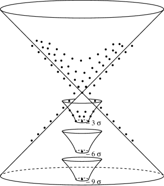
Figure 1: Schematic representation of the roots of $E_{10}$ in the Lorentzian space of the Cartan degrees of freedom $\beta$. Positive roots are in the upper part of the figure, while negative ones are in the lower part. The real roots are on the outer (timelike) hyperboloid $\alpha^{2}=+2$. The imaginary roots are either null ($\alpha^{2}=0$) or timelike ($\alpha^{2}=-2j$). The basic root associated with the leading $R^{4}$ correction to the supergravity action is the negative, timelike point $-3\sigma$ indicated. From it stems the solid half-hyperboloid of roots associated with subleading contributions contained in $R^{4}$ as well as in the other 8th order derivative terms: $R^{2}(DF)^{2}$, $R(DF)^{3}$, $(DF)^{4}$, $\cdots,F^{8}$, as well as the Chern-Simons contribution $AR^{4}$. Similar half-hyperboloids stem from the roots $-3k\sigma$ predicted to exist and to be associated to higher-order contributions $\sim R^{7},R^{10},\cdots$

The reasoning above shows only that the wall forms are of the form (80) for some non-negative integers $n_{i}$. The tools we used above are too coarse to determine whether all values of the integers $n_{i}$ are realized, or whether there are restrictions of any kind on the values of the $n_{i}$’s. In view of the complicated structure of the higher-order corrections, which as we pointed out, is not known in an algebraically completely reduced form, especially for the crucial next-to-leading terms $R^{2}(DF)^{2}$ and $R^{3}F^{2}$), we have made no attempt at an exhaustive analysis as to whether the integers $n_{i}$ are indeed subject to restrictions. Instead, we have proceeded ‘experimentally’ by studying in detail some specific, but typical, terms that we could check to be indeed present among the available expressions for various higher-order corrections. In all the cases we have checked, we did find a rather remarkable pattern: the vector in root space joining the ‘leading ’ $R^{4}$ root $\alpha_{\rm leading}=-3\sigma$ to any subleading higher-order wall form $w_{\rm subleading}$, i.e. the quantity

$$\zeta:=w_{\rm subleading}-\alpha_{\rm leading}=\sum n_{i}\alpha_{i}$$ (81)

was ‘experimentally’ found to satisfy the restriction

$$\zeta^{2}\equiv\left(\sum n_{i}\alpha_{i}\right)^{2}\leq 2$$ (82)

in all cases. Below, we will refer to $\zeta$ as the ‘relative vector’. This leads us to formulate the following

Conjecture: The relation (82) holds for all kinematically allowed combinations, and thereby encodes information about the algebraic structure of the 8th order corrections.

We shall illustrate below with some examples the interrelation between this conjecture and the properties of the $E_{10}$ root lattice on the one hand, and certain ‘kinematical cancellations’, as they follow from the kinematical structure of the known 8th order correction terms, on the other hand. However, we will leave a systematic investigation of this aspect to future work.

Geometrically, the restriction (82) (together with $n_{i}\geq 0$) means that the relative position vector $\zeta$, Eq. (81), belongs to the set of positive roots, $\Delta_{+}$. In other words, if we assume that this restriction is indeed true for all terms, we can geometrically describe the set of wall forms generated by higher-order corrections as a solid half-hyperboloid, which is congruent to $\Delta_{+}$, and with the leading $R^{4}$ root $\alpha_{\rm leading}=-3\sigma$ as its basis, see Figure 1. From this picture there seems to be no evident upper limit on the height $\sum n_{i}$ of the relative vector (81). We initially thought that the wall forms $w_{\rm subleading}$ might be constrained to lie inside the root diagram stricto sensu (instead of lying anywhere in the root lattice), which would have implied the further restriction $(w_{\rm subleading})^{2}\leq 2$. However, as we shall see below, we found wall forms lying high enough in the solid half-hyperboloid (82) to extend beyond the outer hyperboloid $w^{2}=2$ corresponding to real roots. More precisely, by adding simple roots of $A_{9}$ one generates ${\mathfrak{sl}}_{10}$ weight diagrams starting at a certain highest weight inside this solid half-hyperboloid. Many of the ${\mathfrak{sl}}_{10}$ weight diagrams are such that only a subset of the weights are actually roots of $E_{10}$, while the weight diagram itself extends beyond the hyperboloid $w^{2}=2$. We emphasize that there is no a priori inconsistency or incompatibility in this feature: indeed, starting from a Hamiltonian containing only roots as wall forms, any change of parametrization can generate arbitrary combinations of the roots, and therefore arbitrary elements of the root lattice.

Let us now substantiate our conjecture (82) by giving examples of wall forms associated by various higher-order contributions. We first consider the Chern Simons term in (41), which is proportional to

$$\varepsilon^{ABCD_{1}\dots D_{8}}A_{ABC}{R_{D_{1}D_{2}}}^{E_{1}E_{2}}\cdots{R_{D_{7}D_{8}}}^{E_{7}E_{8}}t^{(8)}_{E_{1}\cdots E_{8}}$$

$$\qquad\qquad\equiv\varepsilon_{11}A_{3}\left[24\,{\rm tr}\,R^{4}-6\,({\rm tr}\,R^{2})^{2}\right]$$ (83)

Here the tensor $t_{8}$ is, by virtue of (42), equivalent to the combination of traces appearing in (41). Though the above contribution is also quartic in the curvature, and contains the spatial components $A_{abc}$ of the three-form which simply freeze near the singularity, it is actually subleading w.r.t. the leading curvature contribution $\sim ER^{4}\sim e^{6\sigma}$. The reason for this is the interplay of the $\varepsilon$ tensor, which constrains the first pairs of indices $[D_{1}D_{2}]\cdots[D_{7}D_{8}]$ on the curvature tensors to be all different, with the effect of the $t_{8}$ tensor, which contains Kronecker deltas and thereby obliges the remaining indices on the curvature tensors to coincide pairwise. As a consequence, it is not possible to have only leading curvature components of the type $R_{0a0a}$ or $R_{abab}$. A typical contribution is

$$EA_{89\,10}R_{0101}R_{0123}R_{0145}R_{0167}\sim e^{3\sigma+3\beta^{1}+\beta^{2}-\beta^{3}+\beta^{4}-\beta^{5}+\beta^{6}-\beta^{7}-\beta^{8}-\beta^{9}-\beta^{10}}$$ (84)

where we used (47). After reshuffling some indices, we obtain the wall form

$$w=-(3,2,2,2,1,1,1,1,1,1)\quad\Longleftrightarrow\quad w=-[5\,;\,2,5,8,6,5,4,3,2,1]$$ (85)

This is a root because $w^{2}=2$, with $\ell=-5$. The corresponding relative vector

$$\zeta=w-\alpha_{\rm leading}\equiv w+3\sigma=(0,1,1,1,2,2,2,2,2,2)$$ (86)

satisfies $(w+3\sigma)^{2}=+2$, in agreement with (82). We thus see that this Chern Simons wall form is so much higher than the basic $R^{4}$ root $-3\sigma$ that the associated wall form lies even beyond the interior of the past CSA lightcone and belongs to the timelike hyperboloid $\alpha^{2}=+2$.

Next we consider the subleading curvature terms. Let us first recall that the kinematic structure of the $C^{4}$ terms in (44) eliminates certain combinations; for instance, from (73) it is obvious that there are no contributions of the type $C_{abab}^{4}$ (no summation on indices $a,b$). As is evident from (50), the curvature terms coming from $R^{(2)}_{abcd}$ and the above estimates are strongly suppressed. Furthermore, not all of them produce actual roots, as we shall see presently.

Obviously, from (50), there are many such terms, which we can group into certain ‘permutation multiplets’. A first set of terms corresponds to terms of type

$$ER^{(2)}_{abcd}R^{(2)}_{abef}R^{(2)}_{cegh}R^{(2)}_{dfgh} \sim e^{-2\sigma}\cdot e^{\beta^{a}+\beta^{b}+\beta^{c}-\beta^{d}}\cdot e^{\beta^{a}+\beta^{b}+\beta^{e}+\beta^{f}-2\beta^{i}}$$ (87)

$$\cdot e^{\beta^{c}+\beta^{e}+\beta^{g}+\beta^{h}-2\beta^{j}}\cdot e^{\beta^{d}+\beta^{f}+\beta^{g}+\beta^{h}-2\beta^{k}}$$

We can write this result schematically as

$$E\left[R^{(2)}\right]^{4}\sim e^{-2\sigma}\cdot e^{2(\beta^{a}+\beta^{b}+\beta^{c}+\beta^{e}+\beta^{f}+\beta^{g}+\beta^{h}-\beta^{i}-\beta^{j}-\beta^{k})}$$ (88)

Taking the indices to be all different, and choosing $(i,j,k)=(8,9,10)$, this gives

$$w=-(0,0,0,0,0,0,0,2,2,2)\quad\Longleftrightarrow\quad w=-[2\,;\,2,4,6,6,6,6,6,4,2]$$ (89)

which is clearly not a root as $w^{2}=+8$. Nevertheless, the relative vector

$$\zeta=w+3\sigma=(3,3,3,3,3,3,3,1,1,1)$$ (90)

obeys $\zeta^{2}=2$ and therefore lies on the boundary of the half-hyperboloid in agreement with our conjecture. A second set of terms derives from

$$E\left[R^{(2)}\right]^{4}\sim e^{-2\sigma}\cdot e^{+2(\beta^{a}+\beta^{b}+\beta^{c}+\beta^{d}+\beta^{e}+\beta^{f}-\beta^{g}-\beta^{h})}$$ (91)

and differs from the one above by one symmetry wall. Again taking all indices different and choosing them appropriately, we get

$$w=-(0,0,0,0,0,0,1,1,2,2)\quad\Longleftrightarrow\quad w=-[2\,;\,2,4,5,6,6,6,6,4,2]$$ (92)

which is again not a root as $w^{2}=+6$. The relative vector

$$\zeta=w+3\sigma=(3,3,3,3,3,3,2,2,1,1)$$ (93)

is lightlike, $\zeta^{2}=0$, and lies within the half-hyperboloid. A third set of terms comes from

$$E\left[R^{(2)}\right]^{4}\sim e^{-2\sigma}\cdot e^{+2(\beta^{a}+\beta^{b}+\beta^{c}+\beta^{e}+\beta^{g}-\beta^{h})}$$ (94)

and gives rise to, choosing values for the indices conveniently,

$$w=-(0,0,0,0,0,1,1,1,1,2)\quad\Longleftrightarrow\quad w=-[2\,;\,2,4,6,6,6,5,4,3,2]$$ (95)

with $w^{2}=+4$, and

$$\zeta=(3,3,3,3,3,2,2,2,2,1)$$ (96)

with $\zeta^{2}=-2$. Finally, there is a fourth set with

$$w=-(0,0,0,0,1,1,1,1,1,1)\quad\Longleftrightarrow\quad w=-[2\,;\,2,4,6,6,5,4,3,2,1]$$ (97)

which now is a root because $w^{2}=2$, and

$$\zeta=(3,3,3,3,2,2,2,2,2,2)\quad\Rightarrow\quad\zeta^{2}=-4$$ (98)

again confirming the conjecture. The maximal height for any of these wall forms $w$ is $-44$ for (89), well above the height $-115$ computed above for the leading term, see Figure 1. We observe that all of the terms displayed above differ from one another either by simple permutations of the wall form components, or by the addition of symmetry roots.

Similar comments apply to the curvature terms with one or more temporal indices. From (44), we find, for instance, that terms $\propto(C_{0abc})^{4}$ or $(C_{0abc})^{2}(C_{0ade})^{2}$, with the indices $a,b,c,d,e$ all different (and no summation on repeated indices!), cancel between the two contributions in (44). Remarkably, these terms are precisely of a form which is disallowed by our conjecture above: for instance, if the term

$$E(R_{01ab})^{2}(R_{01cd})^{2}\sim e^{-2\sigma}\cdot\left(e^{\sigma+\beta^{1}+\beta^{a}-\beta^{b}}\right)^{2}\left(e^{\sigma+\beta^{1}+\beta^{c}-\beta^{d}}\right)^{2}$$ (99)

with $a,b,c,d$ all different, had contributed instead of cancelling, it would have yielded (choosing indices conveniently)

$$w=-(3,2,2,1,1,1,1,1,0,0)\quad\Rightarrow\quad\zeta=(0,1,1,2,2,2,2,2,3,3)$$ (100)

whence $\zeta^{2}=+4$, in violation of (82).

A set of terms which does contribute, by inspection of (44), is

$$E(R_{01ab})^{2}(R_{0101})^{2}\sim e^{4\sigma-2\beta^{1}+2\beta^{a}+2\beta^{b}}$$ (101)

Choosing $(a,b)=(9,10)$, we get the maximal height contribution

$$w=-(1,2,2,2,2,2,2,2,3,3)\quad\Longleftrightarrow\quad w=-[7\,;\,6,11,16,14,12,10,8,6,3]$$ (102)

at level $\ell=-7$, of height $-93>-115$, and obeying $w^{2}=-2$. The corresponding relative vector is

$$\zeta=(2,1,1,1,1,1,1,1,0,0)\quad\Rightarrow\quad\zeta^{2}=2$$ (103)

and therefore on the boundary of the half-hyperboloid. From the tables of [24] we deduce that the set of roots corresponding to $w$ belongs to the ${\mathfrak{sl}}_{10}$ representation $(010000001)$ with outer multiplicity $\mu=1$.

There are numerous mixed terms involving the curvature and the 4-form field strength, which we again illustrate with some examples (we have checked from [43] that the structures displayed below actually do appear). For instance, the term $E(D_{0}F_{0123})^{2}(D_{0}F_{0456})^{2}$ leads to the $\ell=8$ root

$$w=-(3,3,3,3,2,2,2,2,2,2)\quad\Longleftrightarrow\quad w=-[8\,;\,5,10,15,12,10,8,6,4,2]$$ (104)

with $w^{2}=-4$, and relative vector

$$\zeta=(0,0,0,0,1,1,1,1,1,1)\quad\Rightarrow\quad\zeta^{2}=2$$ (105)

At level $\ell=-8$, it corresponds to the ${\mathfrak{sl}}_{10}$ representation $(0001000000)$ with $\mu=2$. The highest root in the multiplet is

$$w=-(2,2,2,2,2,2,3,3,3,3)\quad\Longleftrightarrow\quad w=-[8\,;\,6,12,18,16,14,12,9,6,3]$$ (106)

of height $-106>-115$, well above the height of the leading $R^{4}$ singlet.

From the $C(DF)^{3}$ terms given in [43] we read off the leading term which is $ED_{0}F_{3456}D_{0}F_{789\,10}D_{a}F_{a012}C_{0b0b}$. The associated root is

$$w=-(2,2,2,2,2,2,2,2,1,1)=-[6\,;\,4,8,12,10,8,6,4,2,1]$$ (107)

with $w^{2}=-2$, and

$$\zeta=(1,1,1,1,1,1,1,1,2,2)\quad\Rightarrow\quad\zeta^{2}=0$$ (108)

The relevant ${\mathfrak{sl}}_{10}$ representation at level $\ell=6$ is $(000000010)$ with $\mu=1$. The maximal height in the representation is again above $-115$.

Our final example is the combination $E(D_{0}F_{0123})^{2}(C_{0a0a})^{2}$. It is associated to the $\ell=9$ root

$$w=-(3,3,3,3,3,3,3,2,2,2)=-[9\,;\,6,12,18,15,12,9,6,4,2]$$ (109)

with relative vector

$$\zeta=(0,0,0,0,0,0,0,1,1,1)\quad\Rightarrow\quad\zeta^{2}=2$$ (110)

Indeed, in agreement with the result (63) above, we see that $\zeta$ is just an electric root. On the other hand, $w^{2}=-6$, and $w$ corresponds to the representation $(000000100)$ with $\mu=4$. The highest root in the multiplet is

$$w=-(2,2,2,3,3,3,3,3,3,3)\quad\Longleftrightarrow\quad\alpha=-[9\,;\,7,14,21,18,15,12,9,6,3]$$ (111)

of height $-114>-115$, barely above the height of the leading singlet $C^{4}$ contribution.

9 Discussion

Our analysis of higher order corrections to M Theory provides further evidence for the validity of the conjecture [8] that the classical (bosonic) dynamics of M theory is ‘dual’ to a one-dimensional $\sigma$-model on the infinite dimensional coset space $E_{10}/K(E_{10})$. In particular, we find it remarkable that the leading wall form associated with the known $R^{4}$ corrections, namely the permutation singlet $w_{4}=-3\sigma$ does match with a root of $E_{10}$ whose corresponding generator is a ${\mathfrak{sl}}_{10}$ singlet. This compatibility between a gravity structure and a Kac-Moody algebra one was not a priori guaranteed, and can be viewed as a deep confirmation of the hidden role of $E_{10}$ in M theory. Indeed, as a foil, let us consider the simple case of pure gravity in any spacetime dimension $D\equiv d+1$. The study of the corresponding cosmological billiard has found that one should associate to pure gravity the Kac-Moody algebra $AE_{d}$ [4]. Now, for pure (bosonic) gravity, one generally expects that the first higher-order corrections will be $\sim(R_{\mu\nu\rho\sigma})^{2}$. However, by using Eq. (69) such terms quadratic in curvature correspond to the wall form $w_{2}=-\,\sigma$ whose squared length is $(w_{2})^{2}=-\,d/(d-1)$. As the latter squared length is never an integer ), we conclude that $w_{2}$ never corresponds to a root of $AE_{d}$. Let us then consider the problem of determining which values, if any, of the non-linearity order $N$, for corrections $\sim R^{N}$, might be compatible with the algebraic structure of $AE_{d}$. For instance, let us consider the case $d=3$ corresponding to the usual $(3+1)$-dimensional Einstein gravity. By using again Eq. (69), one gets the wall form $w_{N}=-\,(N-1)\,\sigma$ whose squared length in $AE_{d}$ is $-\,\frac{d}{d-1}\,(N-1)^{2}$; i.e. $-\,\frac{3}{2}\,(N-1)^{2}$ when $d=3$. One then concludes that one needs $N=2k+1=3,5,7,\ldots$ The lowest candidate for compatibility with $AE_{3}$ is then $\sim R^{3}$. The corresponding wall form is $w_{3}=-\,2\,\sigma=-\,2\,(\beta^{1}+\beta^{2}+\beta^{3})$. Its squared length is $(w_{3})^{2}=-\,6$, and $w_{3}$ is easily seen to correspond to a root $\alpha$ of $AE_{3}$ of level $\ell=3$ w.r.t. the $SL(3)$ subalgebra [5]. However, as in the case discussed above for $E_{10}$, the wall form $w_{3}=-\,2\,(\beta^{1}+\beta^{2}+\beta^{3})$ is invariant under permutations of the spatial indices. Therefore, for the conjectured correspondence between $(3+1)$-dimensional Einstein gravity and $AE_{3}$ to hold, the wall form $w_{3}$ should correspond to a root of $AE_{3}$ which parametrizes a singlet of $SL(3)$. However, by using the results given in Eq. (8.30) of [5] one sees that there is no singlet representation of $AE_{3}$ at level $\ell=3$. This negative result exemplifies that the compatibility found above between $\sim R^{4}$ corrections and the presence of ‘singlet roots’ of $E_{10}$ is rather non trivial, and could well have failed to hold.

Our work has also provided evidence for the ‘no bounce’ behavior of big crunches in M theory, as naively expected from the dual dynamics, i.e. the global structure of null geodesics on $E_{10}/K(E_{10})$. If we admit the validity of this conjecture, what conclusions can we draw for big crunches in M theory? The ‘dual’ description is an infinite affine length null geodesic going towards $\beta\rightarrow\infty$. This suggests that the quantization of the $E_{10}/K(E_{10})$ model will exhibit no information loss at the big crunch. On the other hand, the dictionary of [8, 9] between the supergravity description and the coset description is defined only in the quasi-classical regime $T\gg T_{P}$. BY contrast, the infinite future of the null geodesic motion corresponds to the regime $T\ll T_{P}$. The fact that the dictionary between the two descriptions becomes ill-defined in this limit (and that we find no evidence for a bounce) suggests that the infinite ‘affine life’ near the singularity can only be described in the coset variables. This situation is somewhat reminiscent of the recent results of [50] based on an AdS/CFT analysis of certain cosmological singularities in anti-deSitter solutions of supergravity. [For a contrasting suggestion based, similarly to the $E_{10}$ coset model, on geodesic motion in auxiliary Lorentz spaces, see refs. [16, 17]].

However, we feel that at this stage of development of the $E_{10}/K(E_{10})$ conjecture, speculating on the ultimate quantum fate of big crunches is premature. Many technically challenging tasks remain before one can seriously consider the eventual physical consequences of the dual $E_{10}$ picture. First, one should extend the dictionary to prove the heretofore unseen roots between height 29 and height 115 do match in the two descriptions. Second, it would be interesting to explore in more detail the validity of the conjecture (82), which was ‘experimentally’ observed to hold in quite a few specific cases. If our conjecture could be fully verified for the known 8-th order corrections, this would open the tantalizing possibility that it still holds for higher corrections $\sim(R+DF+F^{2})^{7},(R+DF+F^{2})^{10},\dots$. It would then provide a strong constraint on the algebraic structure of these corrections. As these corrections are very difficult to obtain by conventional methods, the hidden $E_{10}$ structure might be of great help in pinning down their structure.

Finally, among other pressing issues let us also mention: the role of fermions, the consequences of compactifying eleven-dimensional spacetime (which is expected to reduce the continuous symmetry $E_{10}({\bf R})$ to the discrete symmetry $E_{10}({\bf Z})$), and the effect of quantizing the coset model (see, in this respect, also the remarks in the Appendix below). It would furthermore be interesting to explore the link, if any, between the non-compact T-duality symmetries of string theories in presence of Killing vectors (which have been shown to survive the addition of higher-order terms [51]) and the conjectured $E_{10}$ symmetry.

Acknowledgements

We are grateful to Nathalie Deruelle, Thomas Fischbacher, Gary Horowitz, Victor Kac, Axel Kleinschmidt, Kasper Peeters, Jan Plefka and Arkady Tseytlin for useful exchanges of information. Special thanks go to Ofer Gabber for suggesting a nice way to bracket the values of the term $V_{8}$. We wish also to thank Stanley Deser for many enlightening exchanges over the years, and the organizers of the Deserfest where this work was initiated. We are grateful to Marie-Claude Vergne for preparing the figure. H.N. thanks the Institut des Hautes Etudes Scientifiques for hospitality during the maturation of this work, while T.D. thanks the Albert Einstein Institut for its hospitality during its completion.

Appendix

Geodesic deviation and sectional curvature on $\boldmath{E_{10}/K(E_{10})}$

As shown in [8, 5], geodesic motion on the coset space $E_{10}/K(E_{10})$ is formally integrable in the sense that one can exhibit as many constants of motion as degrees of freedom (i.e. a doubly infinite tower ${\mathcal{J}}$) and, moreover, that one can formally write a generic solution of the geodesic equation in terms of the constants of motion ${\mathcal{J}}$. We wish, however, to emphasize here that, even if formally integrable, geodesic motion on $E_{10}/K(E_{10})$ is at the same time strongly chaotic in the sense that it is extremely sensitive to small deviations in the initial conditions. Let us, indeed, consider the ‘geodesic deviation equation’ which governs the deviation $\xi$ between two neighbouring geodesics. For simplicity, we focus on the neighbourhood of a base geodesic lying entirely in the CSA (corresponding to a simple Kasner solution), i.e. where only $\beta^{a}$ and $\pi_{a}$ are excited. This solution is simply described by $\beta^{a}=v^{a}\,t+\beta_{0}^{a}$ where $t$ is an affine parameter, $\beta_{0}^{a}$ some constants and where the ‘velocity’ $v^{a}$ is null: $G_{ab}\,v^{a}\,v^{b}=0$. The other (‘off diagonal’) variables, $\nu,p$, are all zero. The geodesic deviation equation governing the affine-parameter evolution of the deviation vector $\xi$ connecting this geodesic to a neighbouring one can be obtained in two different ways: either by ‘moving’ the base geodesic $\beta^{a}=v^{a}\,t+\beta_{0}^{a}$ by a generic element in the Lie algebra of $E_{10}$, or by computing the appropriate components of the sectional curvature of the symmetric space $E_{10}/K(E_{10})$ and by writing the general geodesic-deviation (Jacobi) equation. We have checked that both methods give the same result. If we decompose the deviation vector $\xi$ in its various components :

$$\mbox{\boldmath$\xi$}=\xi^{a}\,h_{a}+{\sum}_{\alpha,s}\ \xi_{(s)}^{\alpha}(E_{\alpha}^{(s)}+F_{\alpha}^{(s)})/\sqrt{2},$$

where $h_{a}$, $a=1,\ldots,10$, is a basis of the CSA, and where $\xi_{(s)}^{\alpha}$ denote the components along the non-CSA coset directions. The Jacobi equation yields $\ddot{\xi}^{a}=0$, corresponding to a vanishing sectional curvature in the $vv^{\prime}$ two-planes (where $v=v^{a}\,h_{a}$ is the vector tangent to the base geodesic and $v^{\prime}=v^{\prime a}\,h_{a}$ a generic direction in the CSA), and $\ddot{\xi}_{(s)}^{\alpha}=+\,(\alpha(v))^{2}\,\xi_{(s)}^{\alpha}$, corresponding to a sectional curvature

$$\mathcal{R}(v,E_{\alpha}^{+},v,E_{\alpha}^{+})=-\,(\alpha(v))^{2}$$

where $E_{\alpha}^{+}\equiv(E_{\alpha}+F_{\alpha})/\sqrt{2}$ is a unit-norm vector in the ‘transverse’ coset direction associated to the root $\alpha$. [For simplicity, we suppressed the degeneracy index $s$ on $E_{\alpha}^{(s)}$ and $F_{\alpha}^{(s)}$.] Here $\alpha(v)\equiv\alpha_{a}\,v^{a}$ denotes the value of the linear form $\alpha$ acting on the vector $v=v^{a}\,h_{a}$ tangent to the geodesic. The point we wish to emphasize here is two-fold: $(i)$ the sectional curvature $\mathcal{R}(v,E_{\alpha}^{+},v,E_{\alpha}^{+})$   is negative (as for geodesics on hyperbolic space), and $(ii)$ this sectional curvature decreases without limit towards $-\infty$ as the height of the root increases to infinity. This result shows that small deviations from the geodesic exponentially increase with affine length in a manner which becomes faster and faster as we consider components of the deviation in transverse directions corresponding to higher and higher roots. This indicates that geodesics on $E_{10}/K(E_{10})$ are more and more exponentially sensitive to initial conditions as one examines them in directions of increasing heights. This property might play an important role for the quantization of the geodesic motion on $E_{10}/K(E_{10})$. Indeed, we recall that quantum motion for a scalar particle on curved space involve an ambiguous coupling to the scalar curvature, which appears to be given by a formally infinite series for $E_{10}/K(E_{10})$. This suggests that it is important to include fermions in the $E_{10}$ coset model before drawing conclusions about the strong sensitivity of classical geodesic motion on initial conditions.

References

- [1] V.A. Belinskii, I.M. Khalatnikov and E.M. Lifshitz, Adv. Phys. 19, 525 (1970); Adv. Phys. 31, 639 (1982).
- [2] E. Cremmer, B. Julia and J. Scherk, Supergravity Theory in 11 Dimensions, Phys. Lett. B76 (1978) 409–412
- [3] T. Damour and M. Henneaux, , and Arithmetical Chaos in Superstring Cosmology, Phys. Rev. Lett. 86 (2001) 4749–4752, hep-th/0012172
- [4] T. Damour, M. Henneaux, B. Julia and H. Nicolai, Hyperbolic Kac-Moody Algebras and Chaos in Kaluza-Klein Models, Phys. Lett. B509 (2001) 323–330, hep-th/0103094
- [5] T. Damour, M. Henneaux and H. Nicolai, Cosmological Billiards, Class. Quant. Grav. 20 (2003) R145–R200, hep-th/0212256
- [6] V.G. Kac, Infinite Dimensional Lie Algebras, 3rd edn., Cambridge University Press, 1990
- [7] J.H. Conway and N.J.A. Sloane, “Sphere Packings, Lattices and Groups”, Grundlehren der mathematischen Wissenschaften 290, 2nd edition, Springer Verlag, 1991
- [8] T. Damour, M. Henneaux and H. Nicolai, and a small tension expansion of M Theory, Phys. Rev. Lett. 89 (2002): 221601, hep-th/0207267
- [9] T. Damour and H. Nicolai, Eleven dimensional supergravity and the -model at low levels, hep-th/0410245
- [10] B. Julia, In: S. W. Hawking and M. Rocek (eds.), Superspace and Supergravity, Cambridge University Press (1981).
- [11] B. Julia, Kac-Moody Symmetry Of Gravitation And Supergravity Theories, invited talk given at AMS-SIAM Summer Seminar on Applications of Group Theory in Physics and Mathematical Physics, Chicago, Ill., Jul 6–16, 1982; in: Vertex Operators in Mathematics and Physics, Publications of the Mathematical Sciences Research Institute no 3, Springer Verlag (1984).
- [12] P. C. West, and M theory, Class. Quant. Grav. 18, 4443 (2001) [arXiv:hep-th/0104081]
- [13] P.C. West, and central charges, Phys. Lett. B575 (2003) 333, hep-th/0307098; Brane dynamics, central charges and , hep-th/0412336
- [14] B. S. DeWitt, “Quantum Theory Of Gravity. 1. The Canonical Theory,” Phys. Rev. 160 (1967) 1113.
- [15] G.W. Gibbons and P.K. Townsend, Cosmological evolution of degenerate vacua, Nucl. Phys. B282 (1987) 610
- [16] P.K. Townsend and M.N.R. Wohlfarth, Cosmology as geodesic motion, Class. Quant. Grav. 21 (2004) 5375
- [17] J.G. Russo and P.K. Townsend, Cosmology as relativistic particle mechanics: from big crunch to big bang, Class. Quant. Grav. 22 (2005) 737
- [18] J. Brown, O. Ganor and C. Helfgott, M-theory and : Billiards, Branes, and Imaginary Roots, hep-th/0401053
- [19] F. Englert and L. Houart, invariant formulation of gravity and M-theories: Exact BPS solutions, JHEP 0401 (2004) 002 [arXiv:hep-th/0311255]; invariant formulation of gravity and M-theories: Exact intersecting brane solutions, JHEP 0405 (2004) 059 [arXiv:hep-th/0405082].
- [20] F. Englert, M. Henneaux and L. Houart, From very extended to overextended gravity and M theories, hep-th/0412184
- [21] J. E. Humphreys, “Introduction to Lie Algebras and Representation Theory”, Graduate Texts in Mathematics 9, Springer Verlag, 1980
- [22] A. Kleinschmidt and H. Nicolai, and invariant supergravity, JHEP 0407 (2004) 041 [arXiv:hep-th/0407101].
- [23] V. Kac, R. Moody and M. Wakimoto, On , in Differential Geometrical Methods in Theoretical Physics, eds. K. Bleuler and M. Werner, Kluwer Academic Publishers, 1988
- [24] H. Nicolai and T. Fischbacher, Low Level representations of and , in Proceedings of the Ramanujan International Symposium on Kac-Moody Lie Algebras and Related Topics, eds. N. Sthanumoorthy and K.C.Misra, Contemporary Mathematics, Vol. 343, American Mathematical Society, hep-th/0301017
- [25] M. J. Duff, J. T. Liu and R. Minasian, Eleven-dimensional origin of string / string duality: A one-loop test, Nucl. Phys. B 452 (1995) 261 [arXiv:hep-th/9506126].
- [26] K. Peeters, P. Vanhove and A. Westerberg, Supersymmetric higher-derivative actions in ten and eleven dimensions, the associated superalgebras and their formulation in superspace, Class. Quant. Grav. 18 (2001) 843 [arXiv:hep-th/0010167].
- [27] M. Cederwall, U. Gran, M. Nielsen, B.E.W. Nilsson, Manifestly supersymmetric M theory, JHEP 0010 (2000) 041, hep-th/0007035
- [28] P. Howe and D. Tsimpis, On higher order corrections in M theory, JHEP 0309 (2003) 038, hep-th/0305129
- [29] P. S. Howe, R**4 terms in supergravity and M-theory,, arXiv:hep-th/0408177.
- [30] M. B. Green and J. H. Schwarz, Supersymmetric Dual String Theory (III). Loops and renormalization Nucl. Phys. B 198 (1982) 441.
- [31] N. Sakai and Y. Tanii, One Loop Amplitudes And Effective Action In Superstring Theories, Nucl. Phys. B 287 (1987) 457.
- [32] D. J. Gross and E. Witten, Superstring Modifications Of Einstein’s Equations, Nucl. Phys. B 277 (1986) 1.
- [33] M. T. Grisaru and D. Zanon, Sigma Model Superstring Corrections To The Einstein-Hilbert Action, Phys. Lett. B 177 (1986) 347.
- [34] R. C. Myers, Superstring Gravity And Black Holes, Nucl. Phys. B 289 (1987) 701.
- [35] D.J. Gross and J.H. Sloan, The quartic effective action for the heterotic string, Nucl. Phys. B291 (1987) 41–89
- [36] M. B. Green and P. Vanhove, D-instantons, strings and M-theory, Phys. Lett. B 408 (1997) 122 [arXiv:hep-th/9704145].
- [37] M. B. Green, M. Gutperle and P. Vanhove, One loop in eleven dimensions, Phys. Lett. B 409 (1997) 177 [arXiv:hep-th/9706175].
- [38] M.B. Green, H. Kwon and M. Gutperle, JHEP 08 (1999) 012, hep-th/9907155
- [39] A. A. Tseytlin, R**4 terms in 11 dimensions and conformal anomaly of (2,0) theory, Nucl. Phys. B 584, 233 (2000) [arXiv:hep-th/0005072].
- [40] A. Dasgupta, H. Nicolai and J. Plefka, Vertex operators for the supermembrane JHEP 05 (2000) 007, hep-th/0003280
- [41] B. Pioline, H. Nicolai, J. Plefka and A. Waldron, R**4 couplings, the fundamental memebrane and exceptional theta correspondences, JHEP 0103 (2001) 036, hep-th/0102123
- [42] J. Plefka, Vertex operators for the supermembrane and background field matrix theory, Int. J. Mod. Phys. A16 (2001) 660, hep-th/0009193
- [43] S. Deser and D. Seminara, Counterterms and M-Theory Corrections to Supergravity, Phys. Rev. Lett. 82 (1999) 2435; Tree Amplitudes and Two-Loop Counterterms in Supergravity, hep-th/0002241
- [44] S. Fulling, R. King, B. Wybourne and C. Cummins, Class. Quant. Grav. 9 (1992) 1151
- [45] http://wwwmathlabo.univ-poitiers.fr/ maavl/LiE/
- [46] J. H. Schwarz, “Superstring Theory,” Phys. Rept. 89 (1982) 223. As usual we mean by the , 8-index tensor obtained from Eq. (4.A.21) of this Physics Report by dropping the first 8-index tensor contribution on the right-hand side, and by extending the values of the light-cone indices on the remaining tensor contributions to .
- [47] J. G. Russo and A. A. Tseytlin, —sl One-loop four-graviton amplitude in eleven-dimensional supergravity, Nucl. Phys. B 508 (1997) 245 [arXiv:hep-th/9707134].
- [48] D. Peterson and V. G. Kac, Proc. Natl. Acad. Sci. USA 80 (1983) 1778.
- [49] N. Deruelle, On The Approach To The Cosmological Singularity In Quadratic Theories Of Gravity: The Kasner Regimes, Nucl. Phys. B 327 (1989) 253.
- [50] T. Hertog and G.T. Horowitz, Holographic description of AdS cosmologies, hep-th/0503071
- [51] K. A. Meissner, Symmetries of higher-order string gravity actions, Phys. Lett. B 392 (1997) 298 [arXiv:hep-th/9610131].