Einstein-Born-Infeld-dilaton black holes in non-asymptotically flat spacetimes

Abstract

We derive exact magnetically charged, static and spherically symmetric black hole solutions of the four-dimensional Einstein-Born-Infeld-dilaton gravity. These solutions are neither asymptotically flat nor (anti)-de Sitter. The properties of the solutions are discussed. It is shown that the black holes are stable against linear radial perturbations.

1 Introduction

The nonlinear electrodynamics was first introduced by Born and Infeld in 1934 to obtain finite energy density model for the electron [1]. In recent years nonlinear electrodynamics models are attracting much interest, too. The reason is that the nonlinear electrodynamics arises naturally in open strings and $D$-branes [2]-[7]. Nonlinear electrodynamics models coupled to gravity have been discussed in different aspects (see for example [8]-[24] and references therein).

In the present work we consider stringy Einstein-Born-Infeld-dilaton (EBId) gravity described by the action [3]-[6]

$${\cal S}=\int d^{4}x\sqrt{-g}\left[{\cal R}-2g^{\mu\nu}\partial_{\mu}\varphi\partial_{\nu}\varphi+L_{BI}\right]$$ (1)

where ${\cal R}$ is Ricci scalar curvature with respect to the spacetime metric $g_{\mu\nu}$ and $\varphi$ is the dilaton field. The Born-Infeld (BI) part of the action is given by

$$L_{BI}=4be^{2\gamma\varphi}\left[1-\sqrt{1+{e^{-4\gamma\varphi}\over 2b}F^{2}-{e^{-8\gamma\varphi}\over 16b^{2}}\left(F\star F\right)^{2}}\right].$$ (2)

Here $\star F$ is the dual to the Maxwell tensor and $\gamma$ ($\gamma\neq 0$) is the dilaton coupling constant. In the context of the string theory, the (BI) parameter $b$ is related to the string tension $\alpha$ by $b=1/2\pi\alpha$. It should be noted that the EBId action does not posses an electric-magnetic duality. That is why one should expect that the electrically and magnetically charged solutions will be different. Note that in the $b\to\infty$ limit the action (1) reduces to Einstein-Maxwell-dilaton one.

Unfortunately, the field equations yielded by the action (1) are too complicated and there are no exact analytical solutions in four or more dimensions. Exact solutions to the EBId equations are known only in three dimensions [20]. These solutions are non-asymptotically flat and describe three-dimensional black holes.

In the present paper we derive exact non-asymptotically flat and non-(A)dS black hole solutions to the four-dimensional EBId gravity. Such type solutions, which are non-charged or within the framework of linear electrodynamics have attracted much interest in recent years [25]-[35].

2 Basic equations

Here we consider only magnetically charged case for which $F\star F=0$ and that is why we may restrict ourselves to the truncated BI Lagrangian

$$L_{BI}=4be^{2\gamma\varphi}\left[1-\sqrt{1+{e^{-4\gamma\varphi}\over 2b}F^{2}}\right].$$ (3)

It is also convenient to set

$$L_{BI}=4be^{2\gamma\varphi}{\cal L}_{BI}(X)$$ (4)

where

$${\cal L}_{BI}(X) = 1-\sqrt{1+X},$$ (5)

$$X = {e^{-4\gamma\varphi}\over 2b}F^{2}.$$ (6)

The action (1) then yields the following field equations

$${\cal R}_{\mu\nu}=2\partial_{\mu}\varphi\partial_{\nu}\varphi-4e^{-2\gamma\varphi}\partial_{X}{\cal L}_{BI}(X)F_{\mu\beta}F_{\nu}^{\beta}+2be^{2\gamma\varphi}\left[2X\partial_{X}{\cal L}_{BI}(X)-{\cal L}_{BI}(X)\right]g_{\mu\nu},$$ (7)

$$\nabla_{\mu}\left[e^{-2\gamma\varphi}\partial_{X}{\cal L}_{BI}(X)F^{\mu\nu}\right]=0,$$ (8)

$$\nabla_{\mu}\nabla^{\mu}\varphi=2b\gamma e^{2\gamma\varphi}\left[2X\partial_{X}{\cal L}_{BI}(X)-{\cal L}_{BI}(X)\right],$$ (9)

where $\nabla_{\mu}$ is the covariant derivative with respect to the spacetime metric $g_{\mu\nu}$.

The metric of the static and spherically symmetric spacetime can be written in the form

$$ds^{2}=-\lambda(r)dt^{2}+{dr^{2}\over\lambda(r)}+R^{2}(r)\left(d\theta^{2}+\sin^{2}\theta d\phi^{2}\right).$$ (10)

The electromagnetic field is assumed to have the following pure magnetic form

$$F=P\sin\theta d\theta\wedge d\phi$$ (11)

where $P$ is the magnetic charge. Respectively, we obtain for $X$:

$$X=e^{-4\gamma\varphi}{P^{2}\over bR^{4}}.$$ (12)

The field equations reduce to the following system of coupled ordinary differential equations

$${1\over 2}{d\over dr}\left(R^{2}{d\lambda\over dr}\right) = -2be^{2\gamma\varphi}\left[2X\partial_{X}{\cal L}_{BI}(X)-{\cal L}_{BI}(X)\right]R^{2},$$

$$-{1\over R}{d^{2}R\over dr^{2}} = \left({d\varphi\over dr}\right)^{2},$$ (13)

$$1-{1\over 2}{d\over dr}\left(\lambda{dR^{2}\over dr}\right) = -2be^{2\gamma\varphi}{\cal L}_{BI}(X)R^{2},$$

$${d\over dr}\left(R^{2}\lambda{d\varphi\over dr}\right) = 2\gamma be^{2\gamma\varphi}\left[2X\partial_{X}{\cal L}_{BI}(X)-{\cal L}_{BI}(X)\right]R^{2}.$$

3 Black holes with string coupling constant $\gamma=1$

The case $\gamma=1$ is predicted from the (super)string theory. In order to solve the field equations we make the ansatz

$$R^{2}(r)e^{2\varphi}=r^{2}_{0}$$ (14)

where $r_{0}>0$ is a constant. The second equation of (2) then gives

$$R^{2}(r)=R^{2}_{0}\left({r-C\over r_{0}}\right)$$ (15)

where $C$ and $R_{0}>0$ are constants.

The consistency condition for the third and the fourth equation of (2) gives the following algebraic equation for $r_{0}$:

$${1\over r^{2}_{0}}+4bX\partial_{X}{\cal L}_{BI}(X)=0$$ (16)

with $X={P^{2}\over br^{4}_{0}}$. Solving this equation with respect to $r_{0}$ we obtain

$$r^{2}_{0}=2P^{2}\sqrt{1-{P^{2}_{crit}\over P^{2}}}$$ (17)

where $P^{2}_{crit}=1/4b$. Therefore the magnetic charge must satisfy the inequality

$$P^{2}>P^{2}_{crit}.$$ (18)

The existence of critical value $P_{crit}$ for the magnetic charge is a pure nonlinear effect which disappears in the limit to linear electrodynamics when $b\to\infty$.

Finally, for the metric function $\lambda(r)$ we find

$$\lambda(r)=A{r_{0}(r-r_{+})\over R^{2}_{0}}$$ (19)

where

$$A=4b\left[{\cal L}_{BI}(X)-2X\partial_{X}{\cal L}_{BI}(X)\right]r^{2}_{0}>0$$ (20)

and $r_{+}$ is a constant. Below we discuss the physical properties of the solution and, without loss of generality, we set $C=0$.

The solution is not asymptotically flat and in order to define its mass we use the so-called quasilocal formalism [36]. The quasilocal mass is given by

$${\cal M}(r)={1\over 2}{dR^{2}(r)\over dr}\lambda^{1/2}(r)\left[\lambda_{0}^{1/2}(r)-\lambda^{1/2}(r)\right]$$ (21)

where $\lambda_{0}(r)$ is an arbitrary non-negative function which determines the zero of the energy for a background spacetime. If no cosmological horizon is present, the large $r$ limit of (21) determines the asymptotic mass $M$. In our case the natural choice is $\lambda_{0}(r)=Ar_{0}r/R^{2}_{0}$ and we find

$$M={1\over 4}Ar_{+}.$$ (22)

We first consider solutions with positive mass, $M>0$. The Kretschmann scalar is

$${\cal K}={\cal R}_{\mu\nu\alpha\beta}{\cal R}^{\mu\nu\alpha\beta}=4{\cal K}^{2}_{1}+8{\cal K}^{2}_{2}+8{\cal K}^{2}_{3}+4{\cal K}^{2}_{4}$$ (23)

where

$${\cal K}_{1} = {\cal R}^{01}{}_{01}=0,$$

$${\cal K}_{2} = {\cal R}^{02}{}_{02}=-{1\over 4}{Ar_{0}\over R^{2}_{0}r},$$ (24)

$${\cal K}_{3} = {\cal R}^{12}{}_{12}={1\over 4}{Ar_{+}\over R^{2}_{0}r_{0}}\left({r_{0}\over r}\right)^{2},$$

$${\cal K}_{4} = {\cal R}^{23}{}_{23}={1\over R^{2}_{0}}\left({r_{0}\over r}\right)^{2}\left[{r\over r_{0}}-\left({A\over 4}\right){r-r_{+}\over r_{0}}\right].$$

The scalar ${\cal K}$ is singular only for $r=0$ and tends to zero like $1/r^{2}$ for $r\to\infty$. The solution has a regular horizon at $r=r_{+}$ which hides a spacelike singularity located at $r=0$. Note that the dilaton field is regular on the horizon, too. The spacial infinity is conformally null and the solution describes a black hole with the same causal structure as the Schwarzschild spacetime. The temperature and the entropy of the black hole are

$$T = {1\over 4\pi}{d\lambda\over dr}(r_{+})={1\over 4\pi}{Ar_{0}\over R^{2}_{0}},$$ (25)

$$S = \pi R^{2}_{0}{r_{+}\over r_{0}}.$$ (26)

In order to write the first law we should take into account that the constants $R_{0}$,$A$ and $r_{0}$ are, in fact, related to the background, not to the black hole. Then we find

$$dM=TdS$$ (27)

where the variation is with respect to $r_{+}$ only.

The solution with zero mass ($M=0$) is singular with a null singularity at $r=0$. The case $M<0$ corresponds to naked timelike singularities located at $r=0$.

4 Black holes with general dilaton coupling

Here we consider solutions with general dilaton coupling constant $\gamma$. As for the particular case $\gamma=1$ we make the ansatz

$$R^{2}(r)e^{2\gamma\varphi}=r^{2}_{0}$$ (28)

where $r_{0}>0$ is a constant.

Substituting in the equations (2) we obtain the following algebraic equation for $r_{0}$

$${1\over 2r^{2}_{0}}=-(1-\gamma^{2})b{\cal L}_{BI}(X)-2\gamma^{2}bX\partial_{X}{\cal L}_{BI}(X)$$ (29)

where $X={P^{2}\over br^{4}_{0}}$. In more explicit form the algebraic equation is

$$F(z)=1-(1-\gamma^{2})z-\gamma^{2}z^{2}-{P_{crit}\over|P|}\sqrt{1-z^{2}}=0$$ (30)

where

$$z = {1\over\sqrt{1+X}},$$ (31)

$$r^{2}_{0} = 2|PP_{crit}|{z\over\sqrt{1-z^{2}}}.$$ (32)

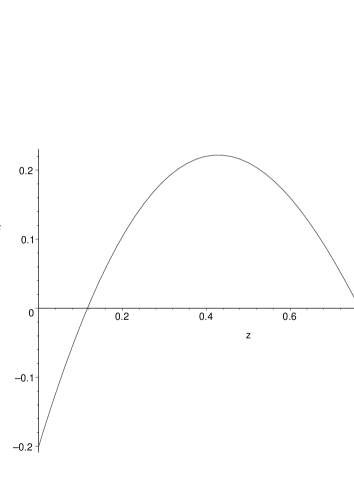
Figure 1: Behavior of the function $F(z)$ for $\gamma=\sqrt{3}$ and ${P_{crit}\over|P|}=1.2$

For sufficiently small $\varepsilon>0$ we have $F(1-\varepsilon)<0$ and, therefore, a sufficient (but not necessary) condition for the algebraic eq. (30) to have roots in the interval $0<z<1$ is $F(0)=1-{P_{crit}\over|P|}>0$. In general, the function $F(z)$ can have zeros also for $P_{crit}>|P|$ and, in some cases, more than one zero as it is shown in the Figure 1 for $\gamma=\sqrt{3}$. Let us note that the different zeros of $F(z)$, in fact, correspond to different backgrounds rather to different black holes, as it is seen from the metric function $\lambda(r)$ presented below.

For the metric functions we find

$$R^{2}(r) = R^{2}_{0}\left({r\over r_{0}}\right)^{{2\gamma^{2}\over 1+\gamma^{2}}},$$ (33)

$$\lambda(r) = A\left({r\over r_{0}}\right)^{{1-\gamma^{2}\over 1+\gamma^{2}}}{r_{0}(r-r_{+})\over R^{2}_{0}},$$ (34)

where $R_{0}>0$ and $r_{+}$ are constants and $A$ is given by

$$A=2(1+\gamma^{2})b\left[{\cal L}_{BI}(X)-2X\partial_{X}{\cal L}_{BI}(X)\right]r^{2}_{0}>0.$$ (35)

The natural background is given by the metric function

$$\lambda_{0}(r)=A\left({r\over r_{0}}\right)^{{1-\gamma^{2}\over 1+\gamma^{2}}}{rr_{0}\over R^{2}_{0}}.$$ (36)

For the asymptotic mass we then obtain

$$M={\gamma^{2}A\over 2(1+\gamma^{2})}r_{+}.$$ (37)

We first consider solutions with positive mass, $M>0$.

The Kretschmann scalar is given by (23) where

$${\cal K}_{1} = {\cal R}^{01}{}_{01}={1-\gamma^{2}\over 1+\gamma^{2}}{A\over R^{2}_{0}}\left({r_{0}\over r}\right)^{{1+3\gamma^{2}\over 1+\gamma^{2}}}\left({\gamma^{2}\over 1+\gamma^{2}}{r-r_{+}\over r_{0}}-{r\over r_{0}}\right),$$

$${\cal K}_{2} = {\cal R}^{02}{}_{02}=-{1\over 2}{\gamma^{2}\over 1+\gamma^{2}}{A\over R^{2}_{0}}\left({r_{0}\over r}\right)^{{1+3\gamma^{2}\over 1+\gamma^{2}}}\left({1-\gamma^{2}\over 1+\gamma^{2}}{r-r_{+}\over r_{0}}+{r\over r_{0}}\right),$$ (38)

$${\cal K}_{3} = {\cal R}^{12}{}_{12}={1\over 2}{\gamma^{2}\over 1+\gamma^{2}}{A\over R^{2}_{0}}\left({r_{0}\over r}\right)^{{1+3\gamma^{2}\over 1+\gamma^{2}}}{r_{+}\over r_{0}},$$

$${\cal K}_{4} = {\cal R}^{23}{}_{23}=-{1\over R^{2}_{0}}\left({r_{0}\over r}\right)^{{1+3\gamma^{2}\over 1+\gamma^{2}}}\left[{\gamma^{4}A\over(1+\gamma^{2})^{2}}{r-r_{+}\over r_{0}}-{r\over r_{0}}\right].$$

The Kretschmann scalar is divergent only for $r=0$ and tends to zero like $r^{-{4\gamma^{2}\over 1+\gamma^{2}}}$ for $r\to\infty$. The solution has a regular horizon at $r=r_{+}$ hiding a spacelike singularity located at $r=0$. For $\gamma^{2}<1$, spacial infinity is conformally timelike and the causal structure is similar to that of the static BTZ black hole spacetime [37]. For $\gamma^{2}\geq 1$, spacial infinity is conformally null and the causal structure is just the same as for the Schwarzschild spacetime. The temperature and the entropy of the black holes are given by

$$T = {Ar_{0}\over 4\pi R^{2}_{0}}\left({r_{+}\over r_{0}}\right)^{{1-\gamma^{2}\over 1+\gamma^{2}}},$$ (39)

$$S = \pi R^{2}_{0}\left({r_{+}\over r_{0}}\right)^{{2\gamma^{2}\over 1+\gamma^{2}}}.$$ (40)

The first law is written in the form

$$dM=TdS$$ (41)

where the variation is with respect to $r_{+}$ only.

The solutions with zero mass are singular with null singularities. The case with negative mass is also singular with null singularities for $\gamma^{2}\leq 1$ and timelike singularities for $\gamma^{2}>1$.

5 Linear stability

The stability of the black holes is an important question from physical point of view. It is well known that there are many black holes solutions which are unstable. Here we show that our black hole solutions are stable against linear radial perturbations. In order to discuss the stability we take the spacetime metric in the form

$$ds^{2}=-e^{\Gamma}dt^{2}+e^{\chi}dr^{2}+e^{\beta}(d\theta^{2}+\sin^{2}\theta d\phi^{2})$$ (42)

where the functions $\Gamma$, $\chi$ and $\beta$ depend on $r$ and $t$. We assume that the metric functions and the dilaton are small perturbations of the static background

$$\Gamma(r,t)=\ln\lambda(r)+\delta\Gamma(r,t),\,\,\,\,\,\,\,\,\chi(r,t)=-\ln\lambda(r)+\delta\chi(r,t),$$

$$\beta(r,t)=2\ln R(r)+\delta\beta(r,t),\,\,\,\,\,\,\,\varphi(r,t)=\varphi(r)+\delta\varphi(r,t).$$ (43)

The convenient gauge is $\delta\beta(r,t)=0$ (i.e. $e^{\beta}=R^{2}(r)$). The electromagnetic field is given by (11) which solves the electromagnetic equations for the time dependent metric (42), too.

The linearized equations for ${\cal R}_{10}$ and ${\cal R}_{22}$ give

$${1\over 2}\partial_{r}\beta(r)\partial_{t}\delta\chi=2\partial_{r}\varphi(r)\partial_{t}\delta\varphi,$$ (44)

$$\left[1-{\cal R}_{22}^{(0)}\right]\delta\chi-{1\over 4}\lambda(r)e^{\beta(r)}\partial_{r}\beta(r)\left(\partial_{r}\delta\Gamma-\partial_{r}\delta\chi\right)$$

$$=4abe^{2\gamma\varphi(r)}\left[2X\partial_{X}{\cal L}_{BI}(X)-{\cal L}_{BI}(X)\right]e^{\beta}\delta\varphi,$$ (45)

where ${\cal R}_{\mu\nu}^{(0)}$ is the Ricci tensor with respect to the static background. The linearized equation for the dilaton is

$$\nabla_{\mu}^{(0)}{\nabla^{(0)}}^{\mu}\delta\varphi-\left[\nabla_{\mu}^{(0)}{\nabla^{(0)}}^{\mu}\varphi(r)\right]\delta\chi+{1\over 2}\lambda(r)\partial_{r}\varphi(r)\left(\partial_{r}\delta\Gamma-\partial_{r}\delta\chi\right)=$$

$$-4\gamma^{2}be^{2\gamma\varphi(r)}\left[{\cal L}_{BI}(X)+4X^{2}\partial^{2}_{X}{\cal L}_{BI}(X)\right]\delta\varphi$$ (46)

where $\nabla_{\mu}^{(0)}$ is the coderivative operator with respect to the static background.

Integrating the equation (44) we obtain

$$\delta\chi=4{\partial_{r}\varphi(r)\over\partial_{r}\beta(r)}\delta\varphi=-{2\over\gamma}\delta\varphi.$$ (47)

Eliminating the perturbations $\delta\chi$ and $\delta\Gamma$ between Eqs. (5), (47) and (5) we find

$$\nabla_{\mu}^{(0)}{\nabla^{(0)}}^{\mu}\delta\varphi-U(r)\delta\varphi=0$$ (48)

where

$$U(r)=4be^{2\gamma\varphi(r)}\left[{\cal L}_{BI}(X)-2X\partial_{X}{\cal L}_{BI}-\gamma^{2}\left[{\cal L}_{BI}(X)+4X^{2}\partial^{2}_{X}{\cal L}_{BI}(X)\right]\right].$$ (49)

Taking into account the explicit form of the BI Lagrangian it can be shown that $U(r)>0$.

Introducing the new radial coordinate

$$r_{*}=r_{0}r_{+}\int{dr\over\lambda(r)e^{\beta(r)}}=Ar_{0}\ln\left(1-{r_{+}\over r}\right)$$ (50)

the Eq.(48) can be written in the explicit form

$$-{e^{2\beta(r_{*})}\over r^{2}_{0}r^{2}_{+}}\partial^{2}_{t}\delta\varphi+{d^{2}\delta\varphi\over dr^{2}_{*}}-U(r_{*})\lambda(r_{*}){e^{2\beta(r_{*})}\delta\varphi\over r^{2}_{0}r^{2}_{+}}=0$$ (51)

For growing modes $\delta\varphi(r,t)=\delta\varphi(r)e^{\eta t}$ we find

$$-{d^{2}\delta\varphi(r_{*})\over dr^{2}_{*}}+{e^{2\beta(r_{*})}\over r^{2}_{0}r^{2}_{+}}\left[\eta^{2}+U(r_{*})\lambda(r_{*})\right]\delta\varphi(r_{*})=0.$$ (52)

For real $\eta$ the effective potential $U_{eff}={e^{2\beta}\over r^{2}_{0}r^{2}_{+}}\left[\eta^{2}+U\lambda\right]$ is positively defined for $r>r_{+}$. Therefore, there are no bounded solutions for $\delta\varphi$ and we conclude that the black holes are stable against linear radial perturbations.

6 Conclusion

In this paper we derived exact, magnetically charged, static and spherically symmetric black hole solutions to the Einstein-Born-Infeld-dilaton gravity. These solutions are neither asymptotically flat nor (anti)-de Sitter. Some basic properties of the solutions were discussed. It was shown that the black holes are stable against linear radial perturbations. It is worth noting that the black solutions derived in the present paper are solutions not only of the BI electrodynamics but also of general nonlinear electrodynamics described by an arbitrary function ${\cal L}(X)$ provided the corresponding algebraic equations possess roots and the corresponding algebraic inequalities are satisfied. In particular, in the case of the linear electrodynamics with ${\cal L}(X)=-{1\over 2}X$the method presented here gives the well-known non-asymptotically flat and non-(A)dS black hole solutions of Einstein-Maxwell-dilaton (EMd) gravity [29]. Moreover, for ${\cal L}(X)=-{1\over 2}X$ we have $U(r)>0$ and therefore, the EMd black holes are stable against linear radial perturbations for arbitrary dilaton coupling constant $\gamma$.

It is puzzling that the nonlinear electrodynamics equations can be solved for arbitrary function ${\cal L}(X)$. The cause is that we consider the sector where the theory looses a part of its nonlinearity. More precisely, the electromagnetic nonlinearity of the differential equations is transformed into algebraic nonlinearity. This can be explicitly demonstrated as follows. For spherically symmetric magnetic configurations the ansatz (14) and (28) are equivalent to consider $X$ satisfies

$$X=X_{0}=const.$$ (53)

The first consequence following from this fact is that the nonlinear Maxwell equations (7) become linear since the nonlinear part can be pulled out of the equations. In second place, redefining the dilaton field as ${\tilde{\varphi}}=\varphi-\varphi_{0}$ where

$$\varphi_{0}={1\over 2\gamma}\left.\ln\left(2[{\cal L}(X)-2X\partial_{X}{\cal L}(X)]\over X\right)\right|_{X=X_{0}},$$ (54)

the dilaton equation becomes the one of the linear EMd case. The only difference appears in the Einstein equations, which reduce to

$${\cal R}_{\mu\nu}=2\partial_{\mu}{\tilde{\varphi}}\partial_{\nu}{\tilde{\varphi}}+2ke^{-2\gamma{\tilde{\varphi}}}F_{\mu\beta}F_{\nu}^{\beta}-{1\over 2}e^{-2\gamma{\tilde{\varphi}}}F^{2}g_{\mu\nu}$$ (55)

where

$$k=\left.{X\partial_{X}{\cal L}(X)\over 2X\partial_{X}{\cal L}(X)-{\cal L}(X)}\right|_{X=X_{0}}.$$ (56)

In this way we obtained field equations which are linear in the electromagnetic field. Note however, although linear in the electromagnetic field, these equations, in general, are not the EMd equations since $k\neq 1$ for general nonlinear electrodynamics. For example, in the case of the Born-Infeld electrodynamics we have $k\neq 1$ for any finite value of $X_{0}$. Summarizing, we have shown that the all information about the nonlinearity is encoded in the parameter $k$ appearing in the Einstein equations and the nonlinear algebraic constraint (56). It can be seen from the exact solutions presented in the previous sections, that the solutions of the ”k-deformed” EMd equations are quite similar to those of the pure EMd equations. The parameter $k$ influences the background constants in the solutions. In contrast, the nonlinear constraint (56) gives severe physical restrictions on the black holes charge. These restrictions algebraically reflect the nonlinearity of the electromagnetic field. This can be explicitly seen from the solutions for the Born-Infeld electrodynamics with $\gamma=1$ where the constraint (56) gives the existence condition $P^{2}>P^{2}_{crit}$.

References

[1] M. Born and L. Infeld, Proc. R. Soc. London A143, 410 (1934).
[2] E. Fradkin and A. Tseytlin, Phys. Lett. B163, 123 (1985).
[3] R. Matsaev, M. Rahmanov and A. Tseytlin, Phys. Lett. B193, 205 (1987).
[4] E. Bergshoeff, E. Sezgin, C. Pope and P. Townsend, Phys. Lett. B188, 70 (1987).
[5]C. Callan, C. Lovelace, C. Nappi and S. Yost, Nucl. Phys. B308, 221 (1988).
[6] O. Andreev and A. Tseytlin, Nucl. Phys. B311, 221 (1988).
[7] R. Leigh, Mod. Phys. Lett. A4, 2767 (1989).
[8] M. Demianski, Found. Phys. 16, 187 (1986).
[9] D. Wiltshire, Phys. Rev. D38, 244500 (1988).
[10] H. d’Oliveira, Class. Quantum Grav. 11, 1469 (1994).
[11] G. Gibbons and D. Rasheed, Nucl. Phys. B454, 185 (1995).
[12] G. Gibbons and D. Rasheed, Phys. Lett. B476, 515 (1996).
[13] E. Ayon-Beato and A. Garcia, Phys. Rev. Lett. 80, 5056 (1998).
[14] E. Ayon-Beato and A. Garcia, Gen. Relativ. Grav. 31, 629 (1999).
[15] E. Ayon-Beato and A. Garcia, Phys. Lett. B464, 25 (1999).
[16] T. Tamaki and T. Torii, Phys. Rev. D62, 061501R (2000).
[17] G. Clement and D. Gal’tsov, Phys. Rev. D62, 124013 (2000).
[18] T. Tamaki and T. Torii, Phys. Rev. D64, 024027 (2001).
[19] G. Gibbons and C. Herdeiro, Class. Quantum Grav. 18, 1677 (2001).
[20] R. Yamazaki and D. Ida, Phys. Rev. D64, 024009 (2001).
[21] S. Yazadjiev, P. Fiziev, T. Boyadjiev and M. Todorov, Mod. Phys. Lett. A16, 2143 (2001).
[22] M. Gurses and O. Sarioglu, Class. Quantum Grav. 20, 351 (2003).
[23] T. Dey, Phys. Lett. B595, 484 (2004).
[24]R. Cai, D. Pang and A. Wang, Rev. D70, 124034 (2004).
[25] S. Mignemi and D. Wiltshire, Class. Quantum Grav. 6, 987 (1989).
[26] D. Wiltshire, Phys. Rev. D44, 1100 (1991).
[27] S. Mignemi and D. Wiltshire, Phys. Rev. D46, 1475 (1992).
[28] S. Poletti and D. Wiltshire, Phys. Rev. D50, 7260 (1994); D52, 3753(E) (1995).
[29] K. Chan, J. Horne and R. Mann, Nucl. Phys. B447, 441 (1995).
[30] R. Cai, J. Ji and K. Soh, Phys. Rev. D57, 6547 (1998).
[31] R. Cai and Y. Zhang, Phys. Rev. D54, 4891 (1996).
[32] G. Clement, D. Gal’tsov and C. Leygnac, Phys. Rev. D67, 024012 (2003).
[33] G. Clement and C. Leygnac, Phys. Rev. D70, 084018 (2004).
[34] R. Cai and A. Wang, Phys. Rev. D70, 084042 (2004).
[35] S. Yazadjiev, Non-asymptotically flat, non-dS/AdS dyonic black holes in dilaton gravity,
gr-qc/0502024
[36] J. Brown and J. York, Phys. Rev. D47, 1407 (1993).
[37] M. Banados, M. Henneaux and H. Zanelli, Phys. Rev. D48, 1506 (1993).