The fate of (phantom) dark energy universe with string curvature corrections

Abstract

We study the evolution of (phantom) dark energy universe by taking into account the higher-order string corrections to Einstein-Hilbert action with fixed dilaton and modulus fields. While the presence of a cosmological constant gives stable de-Sitter fixed points in the cases of heterotic and bosonic strings, no stable de-Sitter solutions exist when a phantom fluid is present. We find that the universe can exhibit a Big Crunch singularity with a finite time for type II string, whereas it reaches a Big Rip singularity for heterotic and bosonic strings. Thus the fate of dark energy universe crucially depends upon the type of string theory under consideration.

I Introduction

Recent observations suggest that the current universe is dominated by dark energy responsible for an accelerated expansion obser . The equation of state parameter $w$ for dark energy lies in a narrow region around $w=-1$ and may even be smaller than $-1$ Caldwell . When $w$ is less than $-1$, dubbed as phantom dark energy, the universe ends up with a Big Rip singularity Sta ; CKW which is characterized by the divergence of curvature of the universe after a finite interval of time (see Refs. phantom0 ; phantom ).

The energy scale may grow up to the Planck scale in the presence of phantom dark energy. This means that higher-order curvature or quantum corrections can be important around the Big Rip. For example, quantum corrections coming from conformal anomaly are taken into account in Refs. Nojiri for dark energy dynamics. It was found that such corrections can moderate the singularity by providing a negative energy density NOT . Thus it is important to implement quantum effects in order to predict the final fate of the universe.

In low-energy effective string theory there exist higher-curvature corrections to the usual scalar curvature term. The leading quadratic correction corresponds to the product of dilaton/modulus and Gauss-Bonnet (GB) curvature invariant BD . The GB term is topologically invariant in four dimensions and hence does not contribute to dynamical equations of motion if the dilaton/modulus field is constant BB . Meanwhile it affects the cosmological dynamics in presence of dynamically evolving dilaton and modulus fields. The possible effects of the GB term for early universe cosmology and black hole physics were investigated in Refs. GBearly ; AP . Lately the GB correction was applied to the study of cosmological dynamics of dark energy NOS .

When the dilaton and mudulus are fixed, it is important to implement third and next-order string curvature corrections BB . This can change the resulting cosmological dynamics drastically as it happens in the context of inflation Ohta and black holes PKA . The goal of the present paper is to study the effect of next-to-leading order string corrections to the cosmological dynamics around the Big Rip singularity with an assumption that the dilaton and the modulus are stabilized. We would also investigate the existence and the stability of de-Sitter solutions in the presence of a cosmological constant. We shall consider three types of string corrections and study the fate of the universe accordingly.

II Evolution equations

Let us consider the Einstein-Hilbert action in low-energy effective string theory:

$${\cal S}=\int d^{D}x\sqrt{-g}\left[R+{\cal L}_{c}+\ldots\right]\,,$$ (1)

where $R$ is the scalar curvature and ${\cal L}_{c}$ is the string correction which is given by BB

$${\cal L}_{c}=c_{1}\alpha^{\prime}e^{-2\phi}{\cal L}_{2}+c_{2}\alpha^{\prime 2}e^{-4\phi}{\cal L}_{3}+c_{3}\alpha^{\prime 3}e^{-6\phi}{\cal L}_{4}\,,$$ (2)

where $\alpha^{\prime}$ is the string expansion parameter, $\phi$ is the dilaton field, and

$${\cal L}_{2}=\Omega_{2}\,,$$ (3)

$${\cal L}_{3}=2\Omega_{3}+R^{\mu\nu}_{\alpha\beta}R^{\alpha\beta}_{\lambda\rho}R^{\lambda\rho}_{\mu\nu}\,,$$ (4)

$${\cal L}_{4}={\cal L}_{41}-\delta_{H}{\cal L}_{42}-\frac{\delta_{B}}{2}{\cal L}_{43}\,,$$ (5)

with

$$\Omega_{2} = R^{2}-4R_{\mu\nu}R^{\mu\nu}+R_{\mu\nu\alpha\beta}R^{\mu\nu\alpha\beta},$$ (6)

$$\Omega_{3} = R^{\mu\nu}_{\alpha\beta}R^{\alpha\beta}_{\lambda\rho}R^{\lambda\rho}_{\mu\nu}-2R^{\mu\nu}_{\alpha\beta}R_{\nu}^{\lambda\beta\rho}R^{\alpha}_{\rho\mu\lambda}$$ (7)

$$+{3\over 4}RR_{\mu\nu\alpha\beta}^{2}+6R^{\mu\nu\alpha\beta}R_{\alpha\mu}R_{\beta\nu}$$

$$+4R^{\mu\nu}R_{\nu\alpha}R^{\alpha}_{\phantom{\alpha}\mu}-6RR_{\alpha\beta}^{2}+\frac{R^{3}}{4},$$

$${\cal L}_{41} = \zeta(3)R_{\mu\nu\rho\sigma}R^{\alpha\nu\rho\beta}\left(R^{\mu\gamma}_{\delta\beta}R_{\alpha\gamma}^{\delta\sigma}-2R^{\mu\gamma}_{\delta\alpha}R_{\beta\gamma}^{\delta\sigma}\right),$$ (8)

$${\cal L}_{42} = {1\over 8}\left(R_{\mu\nu\alpha\beta}R^{\mu\nu\alpha\beta}\right)^{2}+{1\over 4}R_{\mu\nu}^{\gamma\delta}R_{\gamma\delta}^{\rho\sigma}R_{\rho\sigma}^{\alpha\beta}R_{\alpha\beta}^{\mu\nu}$$ (9)

$$-{1\over 2}R_{\mu\nu}^{\alpha\beta}R_{\alpha\beta}^{\rho\sigma}R^{\mu}_{\sigma\gamma\delta}R_{\rho}^{\nu\gamma\delta}-R_{\mu\nu}^{\alpha\beta}R_{\alpha\beta}^{\rho\nu}R_{\rho\sigma}^{\gamma\delta}R_{\gamma\delta}^{\mu\sigma},$$

$${\cal L}_{43} = \left(R_{\mu\nu\alpha\beta}R^{\mu\nu\alpha\beta}\right)^{2}-10R_{\mu\nu\alpha\beta}R^{\mu\nu\alpha\sigma}R_{\sigma\gamma\delta\rho}R^{\beta\gamma\delta\rho}$$ (10)

$$-R_{\mu\nu\alpha\beta}R^{\mu\nu\rho}_{\sigma}R^{\beta\sigma\gamma\delta}R_{\delta\gamma\rho}^{\alpha}\,.$$

Here one has $\delta_{H(B)}=1$ for heterotic (bosonic) string and zero otherwise. The Gauss-bonnet term, $\Omega_{2}$, as well as the Euler density, $\Omega_{3}$, does not contribute to the background equation of motion for $D=4$ unless the dilaton is dynamically evolving. The coefficients $(c_{1},\ c_{2},\ c_{3})$ are different depending on string theories BB . We have $(c_{1},c_{2},c_{3})=(0,0,1/8),(1/8,0,1/8),(1/4,1/48,1/8)$ for type II, heterotic, and bosonic strings, respectively. In the case of type II string with $D=4$, for example, only the ${\cal L}_{41}$ term affects the dynamical evolution of the system.

We shall consider the flat Friedmann-Robertson-Walker metric with a lapse function $N(t)$:

$$ds^{2}=-N(t)^{2}dt^{2}+a(t)^{2}\sum_{i=1}^{d}(dx^{i})^{2}\,,$$ (11)

where $d=D-1$. The Ricci tensors under this metric are given in the Appendix. In what follows we shall consider the case of $D=4$ under the assumption that the modulus field which corresponds to the radius of extra dimensions is stabilized after the compactification to four dimensions. Then we find

$${\cal L}_{3} = \frac{24}{N^{6}}(H^{6}+I^{3})-\frac{72\dot{N}}{N^{7}}HI^{2}\,,$$ (12)

$${\cal L}_{41} = -\frac{6\zeta(3)}{N^{8}}\left(3H^{8}+4H^{4}I^{2}+4H^{2}I^{3}+I^{4}\right)$$ (13)

$$+\frac{6\zeta(3)\dot{N}}{N^{9}}\left(8H^{5}I+12H^{3}I^{2}+4HI^{3}\right)\,,$$

$${\cal L}_{42} = -\frac{6}{N^{8}}\left(5H^{8}+2H^{4}I^{2}+5I^{4}\right)$$ (14)

$$+\frac{6\dot{N}}{N^{9}}\left(4H^{5}I+20HI^{3}\right)\,,$$

$${\cal L}_{43} = -\frac{6}{N^{8}}\left(60H^{8}+32H^{4}I^{2}+60I^{4}\right)$$ (15)

$$+\frac{6\dot{N}}{N^{9}}\left(64H^{5}I+240HI^{3}\right)\,,$$

where $H\equiv\dot{a}/a$ is the Hubble rate and $I$ is defined by $I\equiv H^{2}+\dot{H}$. It should be noted that, in the case of de-Sitter space time, the expressions (12)-(15) reduce to their counterparts given by Eqs. (27)-(30) in the Appendix.

We shall implement the contribution of a barotropic perfect fluid to the action (1). The equation of state parameter, $w_{m}=p_{m}/\rho_{m}$, is assumed to be constant. Our main interest is to study the final fate of universe filled with a phantom-type fluid ($w_{m}<-1$). In this case the universe eventually reaches a Big Rip singularity Caldwell with a divergent Hubble rate in the absence of higher-curvature terms. We are interested in the effect of string curvature corrections to the cosmological evolution around the Big Rip.

Varying the action (1) with respect to $N$, we find

$$6H^{2}=\rho_{c}+\rho_{m}\,,$$ (16)

where

$$\rho_{c}\equiv\frac{{\rm d}}{{\rm d}t}\left(\frac{\partial{\cal L}_{c}}{\partial\dot{N}}\right)+3H\frac{\partial{\cal L}_{c}}{\partial\dot{N}}-\frac{\partial{\cal L}_{c}}{\partial N}-{\cal L}_{c}\biggr{|}_{N=1}\,.$$ (17)

$\rho_{m}$ is the energy density of the barotropic fluid, satisfying

$$\dot{\rho}_{m}+3H(1+w_{m})\rho_{m}=0\,.$$ (18)

In what follows we shall consider the case with a fixed dilaton. Then we have two dynamical equations (16) and (18) for our system. We note that the variation of the action (1) in terms of the scale factor $a$ gives rise to another equation, but this can be derived from Eqs. (16) and (18) by taking a derivative with respect to $t$. From Eq. (17) we find that the energy density $\rho_{c}$ for type II & heterotic strings is

$$\rho_{c} = B[a_{8}H^{8}+a_{c}I^{4}+a_{4}H^{4}I^{2}+a_{2}H^{2}I^{3}+a_{6}H^{6}I$$ (19)

$$-J(a_{5}H^{5}+a_{1}HI^{2}+a_{3}H^{3}I)]\,,$$

where $J=\ddot{H}+3H\dot{H}+H^{3}$. One has $B=6c_{3}\alpha^{\prime 3}e^{-6\phi}\zeta(3)$, $a_{8}=-21,a_{c}=-3,a_{4}=-12,a_{2}=4,a_{6}=-24,a_{5}=-8,a_{1}=-12,a_{3}=-24$ for type II string, and $B=6c_{3}\alpha^{\prime 3}e^{-6\phi}$, $a_{8}=-21\zeta(3)+35,a_{c}=-3\zeta(3)+15,a_{4}=-12\zeta(3)-6,a_{2}=4\zeta(3)+20,a_{6}=-24\zeta(3)+12,a_{5}=-8\zeta(3)+4,a_{1}=-12\zeta(3)+60,a_{3}=-24\zeta(3)$ for heterotic string. In the case of bosonic strings we have

$$\rho_{c} = A(5H^{6}+2I^{3}-6HIJ)+B[(-21\zeta(3)+210)H^{8}$$ (20)

$$+(-3\zeta(3)+90)I^{4}-(12\zeta(3)+48)H^{4}I^{2}$$

$$+(4\zeta(3)+120)H^{2}I^{3}+(-24\zeta(3)+96)H^{6}I$$

$$+J\{(8\zeta(3)-32)H^{5}+(12\zeta(3)-360)HI^{2}$$

$$+24\zeta(3)H^{3}I\}]\,.$$

where $A=24c_{2}\alpha^{\prime 2}e^{-4\phi}$ and $B=6c_{3}\alpha^{\prime 3}e^{-6\phi}$.

III The fate of dark energy universe

In this section we study the cosmological evolution in dark energy universe for the above three classes of string curvature corrections. Our main interest is the universe dominated by phantom dark energy, but we consider the case of cosmological constant as well. We first study the effects of type II and heterotic corrections and then proceed to the bosonic correction.

III.1 Type II and heterotic strings

For the analysis of dynamics to follow, it would be convenient for us to cast Eqs. (16) and (18) with the correction term (19) in the form:

$$\dot{x} = y\,,$$ (21)

$$\dot{y} = [B\{a_{8}x^{8}+a_{c}I^{4}+a_{4}x^{4}I^{2}+a_{2}x^{2}I^{3}+a_{6}x^{6}I$$ (22)

$$-(3xy+x^{3})\xi\}+z-6x^{2}]/(B\xi)\,,$$

$$\dot{z} = -3(1+w_{m})xz\,,$$ (23)

where $x=H$, $y=\dot{H}$, $z=\rho_{m}$, $I=x^{2}+y$ and $\xi=a_{5}x^{5}+a_{1}xI^{2}+a_{3}x^{3}I$. Here we shall consider the case with $w_{m}\neq-1$. By setting $\dot{x}=0$, $\dot{y}=0$ and $\dot{z}=0$, we find the following de-Sitter fixed point:

$$x_{c}=\left(\frac{6}{BD}\right)^{1/6}\,,~{}~{}y_{c}=0\,,~{}~{}z_{c}=0\,,$$ (24)

where $D=a_{c}+a_{2}+a_{4}+a_{6}+a_{8}-a_{1}-a_{3}-a_{5}$. Since $D<0$ for both type II and heterotic strings, we do not have de-Sitter fixed points.

When a cosmological constant $\Lambda$ is present instead of $\rho_{m}$, corresponding to the equation of state $w_{m}=-1$, we find from Eq. (16) that there exists one de-Sitter solution which satisfies $\Lambda=6H^{2}-BDH^{8}$. One can study the stability of this solution by considering small perturbations $\delta x$ and $\delta y$ about the fixed point. We evaluate two eigenvalues for the matrix of perturbations using the method in Ref. CLW . For the type II correction we find that one eigenvalue is positive while another is negative, thereby indicating that the de-Sitter solution is not stable. Meanwhile in the heterotic case the de-Sitter solution is either a stable spiral (for smaller values of $\Lambda$, see Fig. 1) or a stable node (for larger values of $\Lambda$). We note, however, that this stable solution disappears for the equation of state with $w_{m}\neq-1$.

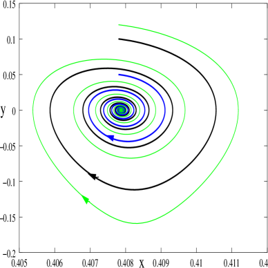
Figure 1: The phase portrait for heterotic string in the case of $\rho_{m}\equiv\Lambda=1$ for several different initial conditions. The stable fixed point $x_{c}\equiv H_{c}=0.408$ corresponds to a de-Sitter solution which is a stable spiral.

Figure 2: The evolution of the Hubble rate $H$ in the presence of string curvature corrections and a phantom fluid with an equation of state: $w_{m}=-1.5$. For the type II correction, the solution approaches $H=-\infty$ by crossing $H=0$, whereas in the heterotic and bosonic cases the Hubble rate grows toward infinity.

In order to understand the fate of the universe which is dominated by a phantom-type fluid, we solve autonomous equations (21)-(23) numerically. Figure 2 shows the evolution of the Hubble rate for a phantom-type fluid with $w_{m}=-1.5$ in the presence of string curvature corrections. We find that in the type II case the Hubble rate begins to decrease because of the presence of string corrections and it eventually diverges toward $-\infty$ after crossing $H=0$. Thus the fate of the universe is characterized by a Big Crunch rather than a Big Rip. Meanwhile in the heterotic case the Hubble rate continues to increase and diverges after a finite interval of time, see Fig. 2. Thus the Big Rip singularity is inevitable even when the heterotic string correction is present.

We also studied cosmological evolution for several different values of $w_{m}$ and for different initial conditions of the Hubble rate. For the type II correction we find that the solutions approach the Big Crunch singularity for $w_{m}\lesssim-1.2$, whereas they tend to approach the Big Rip singularity for $-1.2\lesssim w_{m}<-1$. Thus the fate of the universe depends upon the equation of state for phantom dark energy. For the heterotic case we find that the solutions reach to the Big Rip singularity independent of the values of $w_{m}~{}(<-1)$ and initial conditions of $H$.

III.2 Bosonic string

As demonstrated above, the type II and the heterotic string models do not exhibit de-Sitter solutions for $w_{m}\neq-1$. However, in the case of bosonic string, there exists a de-Sitter fixed point which satisfies the relation

$$B\left[76-12\zeta(3)\right]H^{6}+AH^{4}-6=0\,.$$ (25)

For example one has $H=0.709$ for $A=1/2$ and $B=3/4$. By considering small perturbations around this solution and evaluating three eigenvalues of the $3\times 3$ matrix for the system given by Eqs. (21)-(23) , we find that two of the eigenvalues are positive for $w_{m}<-1$ and one of them is positive for $w_{m}>-1$. Therefore the de-Sitter solution characterized by Eq. (25) does not correspond to a stable attractor for $w_{m}\neq-1$.

In Fig. 2 we plot the evolution of the Hubble rate with bosonic string corrections in the presence of a phantom-type fluid with $w_{m}=-1.5$. The Hubble rate continues to grow and diverges with a finite time as in the case of heterotic string. We also run our numerical code for different values of $w_{m}$ and find that the solutions approach the Big Rip singularity for $w_{m}<-1$.

When a cosmological constant $\Lambda$ is present instead of $\rho_{m}$, de-Sitter solutions satisfy

$$\Lambda=6H^{2}-AH^{6}-B\left[76-12\zeta(3)\right]H^{8}\,.$$ (26)

There exist two solutions for this equation provided that $\Lambda$ ranges in the region $0<\Lambda<f(H_{M})\equiv 6H_{M}^{2}-AH_{M}^{6}-B\left[76-12\zeta(3)\right]H_{M}^{8}$, where $H_{M}$ is the solution for $3AH_{M}^{4}+4B[76-12\zeta(3)]H_{M}^{6}=6$. For example $H_{M}=0.56$ and $f(H_{M})=1.42$ for $A=1/2$ and $B=3/4$. When $\Lambda=1$, one has two de-Sitter solutions characterized by $H=0.417$ and $H=0.652$. We evaluate two eigenvalues of the $2\times 2$ matrix for perturbations $\delta x$ and $\delta y$ around the fixed points. We find a complex conjugate pair of eigenvalues with negative real part for $H=0.417$ making the fixed point a stable spiral. As for the second second critical point corresponding to $H=0.652$, one of the eigenvalues turns out to be positive, which means that the de-Sitter solution is unstable$-$ a saddle in this case (see Fig. 3).

Figure 3: The phase portrait for bosonic string in the presence of a cosmological constant ($\rho_{m}\equiv\Lambda=1$) with $A=1/2$ and $B=3/4$. There exist two de-Sitter fixed points. The point A [$x_{c}=0.417$] corresponds to a stable spiral, whereas the point B [$x_{c}=0.652$] is a saddle.

IV Summary

In this paper we studied the effect of higher-curvature corrections in low-energy effective string theory on the cosmological dynamics in the presence of dark energy fluid. Since the existence of a phantom fluid leads to the growth of the Hubble rate, the energy scale of the universe may reach the Planck scale in future. This means that string curvature corrections can be very important to determine the dynamical evolution of the universe.

We have considered string corrections up to quartic in curvatures for three type of string theories– (i) type II, (ii) heterotic, and (iii) bosonic strings. In our analysis the contribution of the Gauss-Bonnet term does not affect the cosmological dynamics in $D=4$ dimensions, since the dilaton and the modulus fields are fixed. For the fluid with an equation of state characterized by $w_{m}\neq-1$, we find that de-Sitter solutions do not exist for type II and heterotic string corrections. There is a de-Sitter solution for the bosonic string even for $w_{m}\neq-1$, but this is found to be unstable. When the equation of state for fluid is that of a cosmological constant ($w_{m}=-1$), we find that stable de-Sitter solutions exist for heterotic and bosonic strings.

We ran our numerical code to study the effect of string corrections around the Big Rip when a phantom fluid is present. In the type II case we found that the solutions approach the Big Crunch singularity ($H\to-\infty)$ after crossing $H=0$ when the equation of state for dark energy is $w_{m}\lesssim-1.2$. Meanwhile the Hubble rate diverges toward $H\to+\infty$ with a finite time for heterotic and bosonic corrections, which implies that the Big Rip singularity is difficult to be avoided in these cases. The divergent behavior of the Hubble rate for $w_{m}<-1$ is associated with the fact that there are neither stable de-Sitter nor stable Minkowski attractors for the types of the corrections we considered.

In the present letter we restricted our attention to purely geometrical effects assuming that non-perturbative potentials may arise allowing to freeze dilaton and modulus fields. Compactifications from higher dimensions to 4-dimensional space time result in residual modulus fields which are related to the radii of internal space. In general a modulus field is dynamical and interacts with higher-order curvature terms. The same is true for the dilaton field which is related to string coupling $g_{s}$. These may give rise to non-trivial effects, for instance, even the GB curvature invariant which is purely topological in 4 dimensions, does not vanish in the presence of dynamical modulus and dilaton fields. Such a scenario would have important implications for future evolution of the dark energy universe. Very recently, cosmological dynamics based upon effective string theory action was investigated with dynamically evolving modulus and dilaton fields in the presence of second-order curvature corrections Gian (see Ref. Odintsov on the related theme). It was demonstrated that the second-order curvature correction to Einstein-Hilbert action can significantly modify the structure of future singularities in dark energy universe. It is therefore important, though technically cumbersome, to extend the analysis of the present letter to the case of dynamical modulus/dilaton fields.

A comment is also in order about the distinct features that different string models exhibit in cosmological dynamics. With fixed modulus/dilaton, the evolution of phantom dark energy universe is clearly distinguished depending upon string models, namely, the fate of such a universe is Big Crunch for the type II superstring whereas it is a Big Rip for bosonic and heterotic strings. This distinction mainly comes from the difference of the coefficients in Eqs. (19) and (20). In the type II case $\rho_{c}$ becomes negative, which counteracts the energy density of the phantom fluid. This property is crucially important to avoid the Big Rip singularity as pointed out in Ref. NOT . We note that this behavior also appears in the presence of a dynamical modulus field with second-order string corrections Gian . It is really of interest to investigate how the final fate of the universe is changed when dynamical modulus/dilaton fields couples to third/fourth-order string curvature corrections. We hope to address this issue in future work.

In addition, the higher-order curvature contributions used in our description have inbuilt ambiguities related to particular metric redefinitions. It would be important to investigate whether or not these ambiguities can lead to different fate of cosmological evolution.

APPENDIX: Calculation of curvature tensors

For the metric (11) the non-zero components of Christoffel symbols are

$$\Gamma^{0}_{\mu\mu}=\frac{a\dot{a}}{N^{2}}\,,~{}~{}~{}\Gamma^{\mu}_{0\mu}=\Gamma^{\mu}_{\mu 0}=\frac{\dot{a}}{a}\,,~{}~{}~{}\Gamma^{0}_{00}=\frac{\dot{N}}{N}\,,$$

where $\mu=1,2,\ldots d$. By using the formula

$$R^{L}_{SMN}=\partial_{M}\Gamma^{L}_{SN}-\partial_{N}\Gamma^{L}_{SM}+\Gamma^{L}_{MR}\Gamma^{R}_{NS}-\Gamma^{L}_{NR}\Gamma^{R}_{MS}\,,$$

we find that the non-zero components of Riemann tensors are

$$R^{0}_{\mu 0\mu}=-R^{0}_{\mu\mu 0}=\frac{a\ddot{a}}{N^{2}}-\frac{a\dot{a}\dot{N}}{N^{3}}\,,$$

$$R^{\mu}_{00\mu}=-R^{\mu}_{0\mu 0}=\frac{\ddot{a}}{a}-\frac{\dot{a}}{a}\frac{\dot{N}}{N}\,,~{}~{}R^{\mu}_{\nu\mu\nu}=-R^{\mu}_{\nu\nu\mu}=\frac{\dot{a}^{2}}{N^{2}}\,.$$

These give

$$R^{\mu 0}_{0\mu}=R^{0\mu}_{\mu 0}=-R^{\mu 0}_{\mu 0}=-R^{0\mu}_{0\mu}=\frac{1}{N^{2}}\left(\frac{\ddot{a}}{a}-\frac{\dot{a}}{a}\frac{\dot{N}}{N}\right)\,,$$

$$R^{\mu\nu}_{\nu\mu}=-R^{\mu\nu}_{\mu\nu}=\frac{1}{N^{2}}\frac{\dot{a}^{2}}{a^{2}}\,.$$

Noting the relation $R_{MN}=R^{L}_{MLN}$, we obtain

$$R_{00}=-d\left(\frac{\ddot{a}}{a}-\frac{\dot{a}}{a}\frac{\dot{N}}{N}\right)\,,~{}R_{\mu\mu}=\frac{a\ddot{a}}{N^{2}}-\frac{a\dot{a}\dot{N}}{N^{3}}+(d-1)\frac{\dot{a}^{2}}{N^{2}}\,.$$

We also find

$$R_{0\mu\mu 0}=R_{\mu 00\mu}=-R_{0\mu 0\mu}=-R_{\mu 0\mu 0}=a\ddot{a}-a\dot{a}\frac{\dot{N}}{N}\,,$$

$$R_{\mu\nu\mu\nu}=-R_{\mu\nu\nu\mu}=\frac{a^{2}\dot{a}^{2}}{N^{2}}\,,$$

$$R^{0\mu\mu 0}=R^{\mu 00\mu}=-R^{0\mu 0\mu}=-R^{\mu 0\mu 0}=\frac{1}{N^{4}a^{3}}\left(\ddot{a}-\dot{a}\frac{\dot{N}}{N}\right),$$

$$R^{\mu\nu\mu\nu}=-R^{\mu\nu\nu\mu}=\frac{\dot{a}^{2}}{N^{2}a^{6}}\,.$$

These relations are used to evaluate the correction term ${\cal L}_{c}$.

We should note that the corrections can be easily computed in case of de-Sitter symmetry [$R_{abcd}=\Lambda\left(g_{ac}g_{bd}-g_{ad}g_{bc}\right)$], as

$${\cal L}_{3} = 4\Lambda^{3}d(d+1)\,,$$ (27)

$${\cal L}_{41} = -3\zeta(3)\Lambda^{4}(d-1)d(d+1)\,,$$ (28)

$${\cal L}_{42} = \frac{1}{2}\Lambda^{4}(d-7)d^{2}(d+1)\,,$$ (29)

$${\cal L}_{43} = -4\Lambda^{4}d(d+1)\left[1-d(d-9)\right]\,.$$ (30)

These coincide with Eqs. (12)-(15) by setting $N=1$ and $H^{2}=\Lambda$.

References

- (1) S. Hannestad and E. Mortsell, Phys. Rev. D 66, 063508 (2002); A. Melchiorri, L. Mersini, C. J. Odman and M. Trodden, Phys. Rev. D 68, 043509 (2003); J. Weller and A. M. Lewis, Mon. Not. Roy. Astron. Soc. 346, 987 (2003); U. Alam, V. Sahni, T. D. Saini and A. A. Starobinsky, Mon. Not. Roy. Astron. Soc. 354, 275 (2004); P. S. Corasaniti, M. Kunz, D. Parkinson, E. J. Copeland and B. A. Bassett, Phys. Rev. D 70, 083006 (2004).
- (2) R. R. Caldwell, Phys. Lett. B 545, 23 (2002).
- (3) A. A. Starobinsky, Grav. Cosmol. 6, 157 (2000).
- (4) R. R. Caldwell, M. Kamionkowski and N. N. Weinberg, Phys. Rev. Lett. 91, 071301 (2003).
- (5) F. Hoyle, Mon. Not. R. Astr. Soc. 108, 372 (1948); 109, 365 (1949); F. Hoyle and J. V. Narlikar, Proc. Roy. Soc. A282, 191 (1964); Mon. Not. R. Astr. Soc. 155, 305 (1972); 155, 323 (1972); J. V. Narlikar and T. Padmanabhan, Phys. Rev. D 32, 1928 (1985).
- (6) S. M. Carroll, M. Hoffman and M. Trodden, Phys. Rev. D 68, 023509 (2003); S. Nojiri and S. D. Odintsov, Phys. Lett. B 562, 147 (2003); Phys. Lett. B 565, 1 (2003); E. Elizalde, S. Nojiri and S. D. Odintsov, Phys. Rev. D 70, 043539 (2004); P. Singh, M. Sami and N. Dadhich, Phys. Rev. D 68 023522 (2003); M. Sami and A. Toporensky, Mod. Phys. Lett. A 19, 1509 (2004); D. F. Torres, Phys. Rev. D 66, 043522 (2002); V. Sahni and Y. Shtanov, JCAP 0311, 014 (2003); P. F. Gonzalez-Diaz, Phys. Rev. D68, 021303 (2003); Phys. Lett. B 586, 1 (2004); Phys. Rev. D 69, 063522 (2004); P. F. Gonzalez-Diaz and C. L. Siguenza, Nucl. Phys. B 697, 363 (2004); B. Feng, X. L. Wang and X. M. Zhang, Phys. Lett. B 607, 35 (2005); S. Tsujikawa, Class. Quant. Grav. 20, 1991 (2003); J. G. Hao and X. z. Li, Phys. Rev. D 70, 043529 (2004); Phys. Lett. B 606, 7 (2005); M. P. Dabrowski, T. Stachowiak and M. Szydlowski, arXiv:hep-th/0307128; L. P. Chimento and R. Lazkoz, Phys. Rev. Lett. 91, 211301 (2003); arXiv:astro-ph/0405518; V. K. Onemli and R. P. Woodard, Class. Quant. Grav. 19, 4607 (2002); arXiv:gr-qc/0406098; F. Piazza and S. Tsujikawa, JCAP 0407, 004 (2004); A. Feinstein and S. Jhingan, Mod. Phys. Lett. A 19, 457 (2004); H. Stefancic, Phys. Lett. B 586, 5 (2004); arXiv:astro-ph/0312484; X. Meng and P. Wang, arXiv:hep-ph/0311070; H. Q. Lu, arXiv:hep-th/0312082; V. B. Johri, Phys. Rev. D 70, 041303 (2004); astro-ph/0409161; I. Brevik, S. Nojiri, S. D. Odintsov and L. Vanzo, arXiv:hep-th/0401073; J. Lima and J. S. Alcaniz, arXiv:astro-ph/0402265; Z. Guo, Y. Piao and Y. Zhang, arXiv:astro-ph/0404225; M. Bouhmadi-Lopez and J. Jimenez Madrid, arXiv:astro-ph/0404540; J. Aguirregabiria, L. P. Chimento and R. Lazkoz, arXiv:astro-ph/0403157; E. Babichev, V. Dokuchaev and Yu. Eroshenko, arXiv:astro-ph/0407190; Y. Wei and Y. Tian, arXiv:gr-qc/0405038; P. X. N. Wu and H. W. N. Yu, arXiv:astro-ph/0407424; A. Vikman, arXiv:astro-ph/0407107; B. Feng, M. Li, Y-S. Piao and X. m. Zhang, arXiv:astro-ph/0407432; S. M. Carroll, A. De Felice and M. Trodden, arXiv:astro-ph/0408081; C. Csaki, N. Kaloper and J. Terning, arXiv:astro-ph/0409596; Y. Piao and Y. Zhang, Phys. Rev. D 70, 063513 (2004); H. Kim, arXiv:astro-ph/0408577; G. Calcagni, Phys. Rev. D 71, 023511 (2005); P. Avelino, arXiv:astro-ph/0411033; S. Tsujikawa and M. Sami, Phys. Lett. B 603, 113 (2004); J. Q. Xia, B. Feng and X. M. Zhang, arXiv:astro-ph/0411501; I. Ya. Aref’eva, A. S. Koshelev and S. Yu. Vernov, arXiv:astro-ph/0412619; M. Bento, O. Bertolami, N. Santos and A. Sen, arXiv:astro-ph/0412638; S. Nojiri and S. D. Odintsov, arXiv: hep-th/0412030; B. Gumjudpai, T. Naskar, M. Sami and S. Tsujikawa, arXiv:hep-th/0502191; F. Bauer, arXiv:gr-qc/0501078; V. Sahni, arXiv:astro-ph/0502032; F. A. Brito, F. F. Cruz and J. F. N. Oliveira, arXiv:hep-th/0502057; B. McInnes, JHEP 0208, 029 (2002); arXiv:hep-th/0502209; hep-th/0504106; H. Stefancic, arXiv: astro-ph/0504518; L. Perivolaropoulos, arXiv: astro-ph/0504582; A. A. Andrianov, F. Cannata and A. Y. Kamenshchik, arXiv: gr-qc/0505087; L. P. Chimento and D. Pavon, arXiv: gr-qc/0505096; H. Q. Lu, Z. G. Huang and W. Fang, arXiv:hep-th/0504038; G. M. Hossain, arXiv: gr-qc/0503065; I. P. Neupane and D. L. Wiltshire, arXiv: hep-th/0504135.
- (7) S. Nojiri and S. D. Odintsov, Phys. Lett. B 571, 1 (2003); S. Nojiri and S. D. Odintsov, Phys. Lett. B 595, 1 (2004).
- (8) S. Nojiri, S. D. Odintsov and S. Tsujikawa, Phys. Rev. D 71, 063004 (2005).
- (9) D. G. Boulware and S. Deser, Phys. Rev. Lett. 55, 2656 (1985).
- (10) M. C. Bento and O. Bertolami, Phys. Lett. B 368, 198 (1996).
- (11) R. Brustein and R. Madden, Phys. Rev. D 57, 712 (1998); S. Foffa, M. Maggiore and R. Sturani, Nucl. Phys. B 552, 395 (1999); C. Cartier, E. J. Copeland and R. Madden, JHEP 0001, 035 (2000); I. Antoniadis, J. Rizos and K. Tamvakis, Nucl. Phys. B 415, 497 (1994); J. Rizos and K. Tamvakis, Phys. Lett. B 326, 57 (1994); P. Kanti, J. Rizos and K. Tamvakis, Phys. Rev. D 59, 083512 (1999); S. Kawai and J. Soda, Phys. Rev. D 59, 063506 (1999); S. O. Alexeyev, A. V. Toporensky and V. O. Ustiansky, Class. Quant. Grav. 17, 2243 (2000); A. Toporensky and S. Tsujikawa, Phys. Rev. D 65, 123509 (2002); S. Tsujikawa, Phys. Lett. B 526, 179 (2002); S. Tsujikawa, R. Brandenberger and F. Finelli, Phys. Rev. D 66, 083513 (2002).
- (12) S. O. Alexeev and M. V. Pomazanov, Phys. Rev. D 55, 2110 (1997); T. Torii, H. Yajima and K. i. Maeda, Phys. Rev. D 55, 739 (1997).
- (13) S. Nojiri, S. D. Odintsov and M. Sasaki, arXiv:hep-th/0504052.
- (14) K. i. Maeda and N. Ohta, Phys. Lett. B 597, 400 (2004); Phys. Rev. D 71, 063520 (2005); N. Ohta, Int. J. Mod. Phys. A 20, 1 (2005).
- (15) M. Pomazanov, V. Kolubasova and S. Alexeyev, arXiv:gr-qc/0301029.
- (16) E. J. Copeland, A. R. Liddle and D. Wands, Phys. Rev. D 57, 4686 (1998).
- (17) G. Calcagni, S. Tsujikawa and M. Sami, arXiv:hep-th/0505193.
- (18) S. Nojiri, S. D. Odintsov and M. Sasaki, arXiv:hep-th/0504052; S. Nojiri and S. D. Odintsov, arXiv:hep-th/0505215.