What is needed of a tachyon if it is to be the dark energy?

Abstract

We study a dark energy scenario in the presence of a tachyon field $\phi$ with potential $V(\phi)$ and a barotropic perfect fluid. The cosmological dynamics crucially depends on the asymptotic behavior of the quantity $\lambda=-M_{p}V_{\phi}/V^{3/2}$. If $\lambda$ is a constant, which corresponds to an inverse square potential $V(\phi)\propto\phi^{-2}$, there exists one stable critical point that gives an acceleration of the universe at late times. When $\lambda\to 0$ asymptotically, we can have a viable dark energy scenario in which the system approaches an “instantaneous” critical point that dynamically changes with $\lambda$. If $|\lambda|$ approaches infinity asymptotically, the universe does not exhibit an acceleration at late times. In this case, however, we find an interesting possibility that a transient acceleration occurs in a regime where $|\lambda|$ is smaller than of order unity.

I Introduction

There are few more taxing questions facing cosmology today than what is the nature of the dark energy in the Universe? This almost uniform distribution of energy density with a substantial negative pressure completely dominates all other forms of matter and yet the best we can do is to infer its existence from data (see Refs. review for reviews). Moreover, because today it appears to behave just like a cosmological constant, we are naturally led to take seriously the possibility that what we are observing is a remnant of the physics of the very early Universe!

Over the past few years there have been many papers devoted to addressing the nature of the dark energy. Explanations include: a true cosmological constant possibly arising from a Landscape type picture of string vacua KKLT ; dynamical ‘Quintessence’ fields Paul which have tracker like properties where the energy density in the fields track those of the background energy density before dominating today; K-essence scenarios Kes , where the acceleration is driven by modified kinetic terms in the underlying action; modifications of gravity branquint (mainly motivated by Braneworld models) which lead to late time accelerating solutions of the modified Friedmann equation and Chaplygin gas models gas which attempt to incorporate a unified description of dark energy and dark matter. The list goes on, but the aim of all the models is the same, to explain why the Universe has only recently started accelerating with an energy density so close to the critical density.

In this paper, we turn our attention to the issue of the tachyon as a source of the dark energy. The tachyon is an unstable field which has become important in string theory through its role in the Dirac-Born-Infeld (DBI) action which is used to describe the D-brane action as1 ; s1 . A number of authors have already demonstrated that the tachyon could play a useful role in cosmology Tachyonindustry , independent of the fact that it is an unstable field. It can act as a source of dark matter and can lead to a period of inflation depending on the form of the associated potential. Indeed it has been proposed as the source of dark energy for a particular class of potentials Paddy ; Bagla ; AF ; AL ; GZ . However, there has not really been an effort to understand the general properties of tachyonic cosmologies. We attempt to do that here. Starting with the four-dimensional Dirac-Born-Infeld (DBI) action, the tachyon field (with arbitrary potential $V(\phi)$) is coupled to a background perfect fluid of radiation or matter. Modifying the procedure introduced in CLW (see also Refs. vandenHoogen:1999qq ; Billyard:1998hv ; LS ; MP ; NNR ; MM ; Maeda01 ; Huey:2001ae ; Mizuno ; PT ; SST on a related theme), the evolution equations for the system of tachyon plus a background fluid can be written as first order differential equations involving two variables $x$ and $y$ where $x\propto\dot{\phi}$ and $y\propto\sqrt{V(\phi)}/H$, $H$ being the Hubble parameter. Such equations have solutions whose behaviour depends crucially on the quantity $\lambda=-M_{p}V_{\phi}/V^{3/2}$, where $V_{\phi}\equiv{\rm d}V/{\rm d}\phi$. We analyse this behaviour for a wide class of potentials. Depending on the asymptotic behaviour of $\lambda$ we either obtain late time attractor solutions which correspond to the well known inflationary cosmologies associated with the tachyon potential $V(\phi)\propto 1/\phi^{2}$, or perhaps more interesting cosmologies which include (for $\lambda\to 0$) asymptotic behaviour where the system approaches an “instantaneous” critical point that dynamically changes with $\lambda$. For the case where $|\lambda|\to\infty$ asymptotically, the system does not lead to late time acceleration. However, it does show a period of transient acceleration in the regime where $|\lambda|<{\cal O}(1)$. It raises the possibility that we are living in such a transient regime.

The rest of the paper is as follows: Section II introduces the DBI action and the associated equations of motion for the tachyon field including the background perfect fluid. The equations of motion in terms of the new variables $x$, $y$ and $\lambda$ are presented along with the effective equation of state for the tachyon. Potentials which demonstrate the particular asymptotic features of $\lambda={\rm const},\,0$ or $\infty$ are included. Section III considers the particular case of constant $\lambda$ finding all the associated fixed points for the equations of motion and demonstrating their stability before going on to show how the existence restricts the allowed form of the potential for the tachyon. We show how easy it is to obtain late time accelerating solutions in this case. Section IV considers the case $\lambda\to 0$ for both a non-oscillating and oscillating late time evolution of $\phi$, considering a class of potentials that have these features. As before we find it is possible to have late time acceleration and classify the conditions that have to be met by the tachyon potential. Section V does a similar thing but for a class of potentials which lead asymptotically to $\lambda\to\infty$. Although generally we do not have late time inflation, we show there is a novel feature present which is a transient period of inflation for exponential potentials. We summarise in Section VI.

II DBI Model

The Dirac-Born-Infeld type effective 4-dimensional action for our system is described by as1

$${\cal S} = \int d^{4}x\biggl{\{}\sqrt{-g}\frac{M_{p}^{2}}{2}R$$ (1)

$$-V(\phi)\sqrt{-\det(g_{\mu\nu}+\partial_{\mu}\phi\partial_{\nu}\phi)}\biggr{\}}\,,$$

where $M_{p}$ is the reduced Planck mass, $R$ is the scalar curvature and $V(\phi)$ is the potential of the tachyon field $\phi$. The above tachyon DBI action is believed to describe the physics of tachyon condensation for all values of $\phi$ as long as string coupling and the second derivative of $\phi$ are small.

We shall consider a cosmological scenario in which the system is filled with the field $\phi$ and a barotropic perfect fluid with an equation of state $p_{B}=(\gamma-1)\rho_{B}$. Note that $\gamma=1$ for a pressureless dust and $\gamma=4/3$ for radiation. In a spatially flat Friedmann-Lemaitre-Robertson-Walker (FLRW) metric with a scale factor $a$, the pressure and the energy densities of the field $\phi$ are given, respectively, by

$$p_{\phi}=-V(\phi)\sqrt{1-\dot{\phi}^{2}}\,,~{}~{}~{}\rho_{\phi}=\frac{V(\phi)}{\sqrt{1-\dot{\phi}^{2}}}\,.$$ (2)

The background equations of motion are

$$\dot{H}=-\frac{\dot{\phi}^{2}V(\phi)}{2M_{p}^{2}\sqrt{1-\dot{\phi}^{2}}}-\frac{\gamma}{2}\frac{\rho_{B}}{M_{p}^{2}}\,,$$ (3)

$$\frac{\ddot{\phi}}{1-\dot{\phi}^{2}}+3H\dot{\phi}+\frac{V_{\phi}}{V}=0\,,$$ (4)

$$\dot{\rho}_{B}+3\gamma H\rho_{B}=0\,,$$ (5)

together with a constraint equation for the Hubble parameter:

$$3M_{p}^{2}H^{2}=\frac{V(\phi)}{\sqrt{1-\dot{\phi}^{2}}}+\rho_{B}\,.$$ (6)

Let us rewrite the above equations in an autonomous form. We define the following dimensionless quantities:

$$x=\dot{\phi}=H\phi^{\prime}\,,~{}~{}~{}y=\frac{\sqrt{V(\phi)}}{\sqrt{3}HM_{p}}\,,$$ (7)

where a prime denotes the derivative with respect to the number of $e$-folds, $N={\rm ln}\,a$. Then we obtain the following equations:

$$x^{\prime}=-(1-x^{2})(3x-\sqrt{3}\lambda y)\,,$$ (8)

$$y^{\prime}=\frac{y}{2}\left(-\sqrt{3}\lambda xy-\frac{3(\gamma-x^{2})y^{2}}{\sqrt{1-x^{2}}}+3\gamma\right)\,,$$ (9)

$$\lambda^{\prime}=-\sqrt{3}\lambda^{2}xy(\Gamma-3/2)\,,$$ (10)

where

$$\lambda=-\frac{M_{p}V_{\phi}}{V^{3/2}}\,,~{}~{}~{}\Gamma=\frac{VV_{\phi\phi}}{V_{\phi}^{2}}\,.$$ (11)

From Eqs. (3) and (6) we have

$$\frac{H^{\prime}}{H}=-\frac{3}{2}\left[\gamma-\frac{(\gamma-x^{2})y^{2}}{\sqrt{1-x^{2}}}\right]\,.$$ (12)

We also define

$$\Omega_{\phi} \equiv\frac{\rho_{\phi}}{\rho_{\rm cr}}=\frac{V(\phi)}{3M_{p}^{2}H^{2}\sqrt{1-\dot{\phi}^{2}}}=\frac{y^{2}}{\sqrt{1-x^{2}}}\,,$$ (14)

$$\Omega_{B}\equiv\frac{\rho_{B}}{\rho_{\rm cr}}=\frac{\rho_{B}}{3M_{p}^{2}H^{2}}\,,$$

where $\rho_{\rm cr}=3M_{p}^{2}H^{2}$. Note that these satisfy the constraint equation $\Omega_{\phi}+\Omega_{B}=1$ by Eq. (6). Since $0\leq\Omega_{\phi}\leq 1$, the allowed range of $x$ and $y$ is $0\leq x^{2}+y^{4}\leq 1$. Therefore both $x$ and $y$ are finite in the range $0\leq x^{2}\leq 1$ and $0\leq y\leq 1$. The effective equation of state for the field $\phi$ is

$$\gamma_{\phi}=\frac{\rho_{\phi}+p_{\phi}}{\rho_{\phi}}=\dot{\phi}^{2}\,,$$ (15)

which means that $\gamma_{\phi}\geq 0$. The condition for inflation corresponds to $\dot{\phi}^{2}<2/3$ Tachyonindustry . It is also convenient to introduce a standard deceleration parameter as

$$q\equiv-\frac{\ddot{a}a}{\dot{a}^{2}}=\frac{3}{2}\gamma-1-\frac{3}{2}\frac{\gamma-x^{2}}{\sqrt{1-x^{2}}}y^{2}\,.$$ (16)

Equation (10) implies that one can have $\lambda={\rm const}$ for $\Gamma=3/2$. In this case integrating Eq. (11) gives Paddy ; Bagla

$$V(\phi)=M^{2}\phi^{-2}\,.$$ (17)

This corresponds to the potential for scaling solutions in the context of braneworld cosmology Maeda01 ; MM ; SS . Recently a phase-space analysis was performed in Ref. AL for the same potential in the tachyon system. In this paper, we are intend to broaden this type of investigation to allow for the more general situation where the potential is not restricted to Eq. (17). In fact the tachyon potentials we introduce are motivated either by string theory or based purely on phenomenological considerations.

For example, in the case of a general inverse power-law potential abdalla ; AF

$$V(\phi)=M^{4-n}\phi^{-n}\,,$$ (18)

one has $\lambda\propto\phi^{(n-2)/2}$ and $\Gamma=(n+1)/n$. Therefore $\lambda$ is constant for $n=2$, but it dynamically changes for $n\neq 2$. In the limit of $\phi\to\infty$ we have $\lambda\to 0$ for $0<n<2$ and $\lambda\to\infty$ for $n>2$.

It is convenient to classify the potential $V(\phi)$ depending on the asymptotic behavior of $\lambda$ as in the case of a normal scalar field MP . They can be classified as follows:

• (i) $\lambda={\rm const}$.

  In the tachyon system, the inverse square potential $V(\phi)=M^{2}\phi^{-2}$ gives a constant $\lambda$. Note that an exponential potential corresponds to a constant value of $\tilde{\lambda}\equiv-M_{p}V_{\phi}/V$ in the case of a normal scalar field CLW .

• (ii) $\lambda\to 0$ asymptotically.

  There exist a number of potentials that exhibit this behavior. For example

  • (iia) $V=M^{4-n}\phi^{-n}$ with $0<n<2$.

    In this case $\lambda$ ($\propto\phi^{(n-2)/2}$) approaches 0 as $\phi\to\infty$. It is known that inflation occurs for $0<n<2$ AF .

  • (iib) $V=V_{0}e^{1/(\mu\phi)}$.

    This is the potential that is used in the quintessence scenario Paul , and $\lambda\propto e^{-1/(2\mu\phi)}/\phi^{2}$, which satisfies $\lambda\to 0$ as $\phi\to\infty$.

  • (iic) $V(\phi)=V_{0}e^{\frac{1}{2}M^{2}\phi^{2}}$.

    This potential may appear as the excitation of massive scalar fields on the D-brane GST and it has a minimum at $\phi=0$. Since $\lambda\propto\phi e^{-\frac{1}{4}M^{2}\phi^{2}}$ in this case, $\lambda\to 0$ as $\phi\to 0$.

• (iii) $|\lambda|\to\infty$ asymptotically.

  There are also several potentials of interest that give this behavior

  • (iiia) $V=M^{4-n}\phi^{-n}$ with $n>2$.

    As seen earlier, in this case $\lambda$ ($\propto\phi^{(n-2)/2}$) approaches $\infty$ as $\phi\to\infty$.

  • (iiib) $V=V_{0}e^{-\mu\phi}$.

    This potential was considered in Ref. Sami02 in the context of tachyon inflation. Unlike the case of conventional cosmologies, in tachyon cosmology, the exponential potential does not lead to a constant $\lambda$. Since $\lambda$ is proportional to $e^{\frac{1}{2}\mu\phi}$, we find $\lambda\to\infty$ as $\phi\to\infty$. This potential may appear in the late time behaviour of D₃ anti-D₃ cosmology KK1 . The tachyon in the D₃ anti-D₃ system is a complex scalar field $T=\phi e^{i\theta}$ sen2 . When $\theta$ is constant, the effective action of coincident D₃ anti-D₃ is the same as Eq. (1) sen1 . The tachyon potential for the coincident D₃ anti-D₃ is the same as the tachyon potential of non-BPS D₃-brane which is Liu $V(\phi)=2\beta^{2}T_{3}/\cosh(\sqrt{\beta}m\phi)$ where $\beta$ is a warp factor at the position of the D₃ anti-D₃ in the internal compact space, $T_{3}$ is the tension of branes and $m$ is the string mass scale. At the late time ($\phi\to\infty$) the potential behaves as $V(\phi)\sim\beta^{2}T_{3}e^{-\sqrt{\beta}m\phi}$.

  • (iiic) $V(\phi)=V_{0}e^{-\frac{1}{2}M^{2}\phi^{2}}$.

    This is the case in which the tachyon rolls down toward $\phi\to\infty$ unlike the potential (iic). $\lambda$ has a dependence $\lambda=M_{p}M^{2}V_{0}^{-1/2}\phi e^{\frac{1}{4}M^{2}\phi^{2}}$ thereby giving $\lambda\to\infty$ as $\phi\to\infty$.

  It may be noted that the potentials (iiib) $\&$ (iiic) listed above can be obtained in the frame work of string tachyons whereas the inverse power-law type potentials (iiia) are motivated from purely phenomenological considerations.

We can now summarise the above behaviour in terms of conditions on $V(\phi)$. The system approaches $\lambda\to 0$ when the slope of the potential is less steep than that of $V=M^{2}\phi^{-2}$ and the field $\phi$ evolves toward infinity without oscillations [(iia) and (iib)]. The case (iic) corresponds to the one in which the field $\phi$ oscillates as it evolves toward zero asymptotically.

On the other hand, we have an asymptotic value $|\lambda|\to\infty$ when the potential is steeper than that of $V=M^{2}\phi^{-2}$ and the field $\phi$ evolves toward infinity without oscillations [(iiia), (iiib) and (iiic)]. One may consider the potential $V(\phi)=V_{0}(\phi-\phi_{0})^{n}$ , for $n$ positive, that has a dependence $\lambda\propto(\phi-\phi_{0})^{-(n/2+1)}$, thereby showing a divergence of $\lambda$ for $\phi\to\phi_{0}$. However this potential has a number of problems such as a divergent negative mass $m_{\rm eff}^{2}=({\rm log}\,V)_{\phi\phi}$ as $\phi\to\phi_{0}$, which leads to a violent instability of perturbations in the context of tachyon cosmology Frolov . We do not regard this as a realistic dark energy tachyon potential. Note that if the potential has a positive constant energy at $\phi=\phi_{0}$ then this system reduces to that of the case (iic).

III Constant $\lambda$

Let us first consider the situation in which $\lambda$ is constant, i.e., case (i) in the previous section. The fixed points for this system can be obtained by setting $x^{\prime}=0$ and $y^{\prime}=0$ in Eqs. (8) and (9). These are summarized in Table I. Essentially we have 4 fixed points: (a) $x=0$, $y=0$, (b) $x=\pm 1$, $y=0$, (c) $x=\lambda y_{s}/\sqrt{3}$, $y=y_{s}$ and (d) $x=\sqrt{\gamma}$, $y=\pm\sqrt{3\gamma}/\lambda$. Here $y_{s}$ is defined by

$$y_{s}=\left(\frac{\sqrt{\lambda^{4}+36}-\lambda^{2}}{6}\right)^{1/2}\,.$$ (19)

The cases (b) and (d) are divided into two cases, respectively, depending on the signs of $x$. The cases (c) and (d) correspond to stable fixed points. These satisfy the conditions $3x=\sqrt{3}\lambda y$ and $3\gamma=\sqrt{3}\lambda xy+\frac{3(\gamma-x^{2})y^{2}}{\sqrt{1-x^{2}}}$ in Eqs. (8) and (9).

Name	$x$	$y$	Existence	Stability	$\Omega_{\phi}$	$\gamma_{\phi}$
(a)	0	0	All $\lambda$ and $\gamma$	Unstable saddle for $\gamma>0$	0	0
				Stable node for $\gamma=0$
(b1)	1	0	All $\lambda$ and $\gamma$	Unstable node	1	1
(b2)	$-1$	0	All $\lambda$ and $\gamma$	Unstable node	1	1
(c)	$\lambda y_{s}/\sqrt{3}$	$y_{s}$	All $\lambda$ and $\gamma$	Stable node for $\gamma\geq\gamma_{s}$	1	$\lambda^{2}y_{s}^{2}/3$
				Unstable saddle for $\gamma<\gamma_{s}$
(d1)	$\sqrt{\gamma}$	$\sqrt{3\gamma}/\lambda$	$\lambda>0$ and $\gamma<\gamma_{s}$	Stable node	$\frac{3\gamma}{\lambda^{2}}\frac{1}{\sqrt{1-\gamma}}$	$\gamma$
(d2)	$-\sqrt{\gamma}$	$-\sqrt{3\gamma}/\lambda$	$\lambda<0$ and $\gamma<\gamma_{s}$	Stable node	$\frac{3\gamma}{\lambda^{2}}\frac{1}{\sqrt{1-\gamma}}$	$\gamma$

Table 1: The critical points for constant $\lambda$

III.1 Stability of the fixed point solutions

We now study the stability around the critical points given in Table I. Consider small perturbations $u$ and $v$ about the points $(x_{c},y_{c})$, i.e.,

$$x=x_{c}+u\,,~{}~{}~{}y=y_{c}+v\,.$$ (20)

Substituting into Eqs. (8) and (9), leads to the first-order differential equations:

$$\left(\begin{array}[]{c}u^{\prime}\\ v^{\prime}\end{array}\right)={\cal M}\left(\begin{array}[]{c}u\\ v\end{array}\right)\ ,$$ (25)

where ${\cal M}$ is a matrix that depends upon $x_{c}$ and $y_{c}$.

The system can be regarded as being perturbatively stable when the the eigenvalues of the matrix ${\cal M}$ are both negative CLW . In what follows we shall obtain the eigenvalues $\mu_{1}$ and $\mu_{2}$ for the fixed points in Table I and discuss their stability.

• Case (a) [$x_{c}=0$, $y_{c}=0$]:

  The eigenvalues are

  $$\mu_{1}=-3\,,~{}~{}~{}\mu_{2}=3\gamma/2\,.$$ (26)

  Therefore this critical point is an unstable saddle for $\gamma>0$, whereas it is a stable node for $\gamma=0$. This fixed point can not be used as a late-time attractor solution, since it leads to $\Omega_{\phi}=0$.

• Case (b) [$x_{c}=\pm 1$, $y_{c}=0$]:

  Since the eigenvalues are

  $$\mu_{1}=6\,,~{}~{}~{}\mu_{2}=3\gamma/2\,,$$ (27)

  this fixed point is an unstable node. This corresponds to a dust-like solution with $\gamma_{\phi}=\dot{\phi}^{2}=1$, but the system tends to repel from this critical point.

• Case (c) [$x_{c}=\lambda y_{s}/\sqrt{3}$, $y_{c}=y_{s}$]:

  The eigenvalues are

  $$\mu_{1} = -3+\frac{\lambda^{2}}{12}(\sqrt{\lambda^{4}+36}-\lambda^{2})\,,$$ (28)

  $$\mu_{2} = -3\gamma+\frac{\lambda^{2}}{6}(\sqrt{\lambda^{4}+36}-\lambda^{2})\,,$$ (29)

  where $\mu_{1}$ ranges between $-3\leq\mu_{1}<-3/2$. We have $\mu_{2}\leq 0$ for

  $$\gamma\geq\gamma_{s}\equiv\frac{\lambda^{2}}{18}(\sqrt{\lambda^{4}+36}-\lambda^{2})\,.$$ (30)

  This means that the fixed point is a stable node for $\gamma\geq\gamma_{s}$, whereas it is an unstable saddle point for $\gamma<\gamma_{s}$.

• Case (d) [$x_{c}=\pm\sqrt{\gamma}$, $y_{c}=\pm\sqrt{3\gamma}/\lambda$]:

  The eigenvalues are

  $$\mu_{1,2}=\frac{3}{4}\biggl{[}\gamma-2\pm\sqrt{17\gamma^{2}-20\gamma+4+\frac{48}{\lambda^{2}}\gamma^{2}\sqrt{1-\gamma}}\biggr{]}.$$

  The real parts of $\mu_{1}$ and $\mu_{2}$ are both negative if the condition

  $$0\leq\gamma\leq\gamma_{s}=\frac{\lambda^{2}}{18}(\sqrt{\lambda^{4}+36}-\lambda^{2})\,,$$ (32)

  is satisfied. Note that $\gamma_{s}$ is always smaller than 1. When the square root in Eq. (• ‣ III.1) is positive, the fixed point is a stable node. The fixed point is a stable spiral when the square root in Eq. (• ‣ III.1) is negative.

  The values $\Omega_{\phi}$ and $\gamma_{\phi}$ at the critical point are

  $$\Omega_{\phi}=\frac{3\gamma}{\lambda^{2}}\frac{1}{\sqrt{1-\gamma}}\,,~{}~{}~{}\gamma_{\phi}=\gamma\,,$$ (33)

  which corresponds to a scaling solution in which the energy densities $\rho_{\phi}$ and $\rho_{B}$ decrease with the same rate. However we need to caution the reader in that the scaling solution does not exist in the either the matter ($\gamma=1$) or radiation dominated ($\gamma=4/3$) eras, because the existence of the scaling solution requires the condition $0\leq\gamma\leq\gamma_{s}<1$. In this sense this solution can not be applied as a realistic model of dark energy.

III.2 The existence of scaling solutions

It was shown in Ref. PT that the existence of scaling solutions restricts the form of the Lagrangian of a scalar field $\varphi$ to be

$$p(X,\varphi)=X\,g(Xe^{\lambda\varphi})\,,$$ (34)

where $X=-g^{\mu\nu}\partial_{\mu}\varphi\partial_{\nu}\varphi/2$ and $g$ is any function of $Xe^{\lambda\varphi}$. Equation (34) was derived by starting from a general Lagrangian $p(X,\varphi)$ which is an arbitrary function of $X$ and $\varphi$. Recently this result was extended to a more general background given by $H^{2}\propto\rho^{n}$ SS .

The Lagrangian of our tachyon system is

$$p(X,\phi)=-V(\phi)\sqrt{1-2\tilde{X}}\,,$$ (35)

where $\tilde{X}=-g^{\mu\nu}\partial_{\mu}\phi\partial_{\nu}\phi/2$. At first glance it seems that this lagrangian does not satisfy the condition for the existence of scaling solutions given in Eq. (34). However we have earlier shown that this tachyon system (35) does in fact possess scaling solutions given by Eq. (33).

One can clarify the situation by expressing the Lagrangian (34) in terms of the variable $\phi\equiv(2/\lambda)\,e^{\lambda\varphi/2}$. Then Eq. (34) becomes

$$p(\tilde{X},\phi)=\frac{4}{\lambda^{2}\phi^{2}}f(\tilde{X})\,,$$ (36)

where $f(\tilde{X})\equiv\tilde{X}\,g(\tilde{X})$. The tachyon system (35) can be accommodated by choosing

$$V(\phi)\propto\phi^{-2}\,,~{}~{}~{}f(\tilde{X})\propto\sqrt{1-2\tilde{X}}\,.$$ (37)

Therefore scaling solutions exist for the Lagrangian (35) in the case of the inverse square potential, as of course we already knew. It is interesting to note that Eq. (34) completely fixes the form of the Lagrangian for the existence of scaling solutions PT ; SS .

III.3 Late time behavior

The cosmological dynamics of the tachyon field with inverse square potential (17) was studied in Ref. Bagla ; AL . In what follows, we would like to clarify several important points concerning the application of this model to dark energy.

Employing slow-roll approximations: $3H\dot{\phi}\simeq-V_{\phi}/V$ and $3M_{p}^{2}H^{2}\simeq V(\phi)$ in a scalar-field dominated universe ($\rho_{\phi}\gg\rho_{B}$), we obtain

$$\dot{\phi}=\frac{2M_{p}}{\sqrt{3}M}\,,$$ (38)

$$a\propto t^{p}\,,~{}~{}{\rm with}~{}~{}p\equiv\frac{1}{2}\left(\frac{M}{M_{p}}\right)^{2}\,,$$ (39)

for the potential (17). In order to have acceleration at late times, we clearly require $p>1$, i.e.,

$$M>\sqrt{2}M_{p}\,.$$ (40)

Furthermore $M$ needs to be much larger than the Planck mass to obtain a significant acceleration ($p\gg 1$). Such a large mass is problematic as we expect general relativity itself to break down in such a regime. This problem is fortunately alleviated for the inverse power-law potential $V=M^{4-n}\phi^{-n}$ with $0<n<2$, as we will see later.

When $n=2$ the parameter $\lambda$ defined in Eq. (11) is a constant and given by

$$\lambda=2\frac{M_{p}}{M}=\sqrt{\frac{2}{p}}\,.$$ (41)

Then we require $\lambda<\sqrt{2}$ for the acceleration. The fixed point (c) in Table I is the only stable attractor solution with an accelerating universe at late times (recall that the fixed point (d) is not a realistic solution). Let us consider the case of $\lambda\ll 1$ (i.e., $p\gg 1$). The fixed point (c) is approximately given as

$$x\simeq\frac{\lambda}{\sqrt{3}}\,,~{}~{}~{}y\simeq 1-\frac{\lambda^{2}}{12}\,,$$ (42)

together with the equation of state

$$\gamma_{\phi}\simeq\frac{\lambda^{2}}{3}=\frac{2}{3p}\,.$$ (43)

The condition for acceleration ($p>1$) translates into $\gamma_{\phi}<2/3$. One can easily verify that the slow-roll solution in Eq. (38) is identical to the critical point (c) given in Eq. (42). Therefore the slow-roll solution (38) is a stable attractor which gives $\Omega_{\phi}=1$ and $\gamma_{\phi}=2/(3p)$.

We note that there is another constraint coming from the energy scale of the tachyon potential. Since the energy density of the tachyon is supposed to be the same order as the present critical density $\rho_{\rm cr}=10^{-47}\,{\rm GeV}^{4}$, we require the condition $M^{2}\phi_{0}^{-2}\simeq\rho_{\rm cr}$. This restricts the present field values to be $\phi_{0}M\gtrsim 10^{60}$.

IV Case of $\lambda\to 0$

In this section we shall study the case in which $\lambda$ dynamically approaches 0. Examples of potentials which exhibit this behavior was presented in section  II. In the limit of $\lambda\to 0$ Eqs. (8) and (9) read

$$x^{\prime}=-3x(1-x^{2})\,,$$ (44)

$$y^{\prime}=-\frac{H^{\prime}}{H}y\,.$$ (45)

By Eq. (44) $x^{\prime}<0$ for $x>0$ and $x^{\prime}>0$ for $x<0$ (note that $x^{2}$ is in the range $0\leq x^{2}\leq 1$). Therefore $x\to 0$. Integrating Eq. (45) gives $y\propto 1/H$, which means that $y$ continues to increase toward $y=1$ as $H$ decreases. Then the attractor solution should correspond to $x=0$ and $y=1$. This discussion neglects the contribution from terms like $\sqrt{3}\lambda y$, but the solution actually approaches the attractor $(x,y)=(0,1)$ for $\lambda\to 0$ as we see below.

While the fixed points we found in the previous section correspond to the case of constant $\lambda$, we may regard these as “instantaneous” critical points as the function $\lambda(N)$ evolves toward 0. The only stable critical point leading to an acceleration at late times is that of case (c) in Table I, where the dynamical critical point around $\lambda(N)=0$ is approximately given by Eq. (42). This approaches $x\to 0$ and $y\to 1$ as $\lambda\to 0$. Note also that $\gamma_{\phi}\to 0$ as $\lambda\to 0$, which corresponds to the equation of state of a cosmological constant. We would like to numerically confirm that the system actually approaches the dynamical critical point. In what follows we classify the situation in two classes: (A) $\lambda\to 0$ without any oscillations of $\phi$ and (B) $\lambda\to 0$ with $\phi$ oscillating.

IV.1 $\lambda\to 0$ with no oscillations of $\phi$

The potentials which lead to this behaviour correspond to (iia) $V(\phi)=M^{4-n}\phi^{-n}$ with $0<n<2$ and (iib) $V(\phi)=V_{0}e^{1/(\mu\phi)}$. In this class of models the field $\phi\to\infty$ without oscillations. As long as the tachyon potential is not steep relative to the inverse square potential, i.e., $n<2$, $\lambda(N)$ asymptotically approaches 0 as $\phi$ increases. This means that the equation of state of the field $\phi$ approaches $\gamma_{\phi}\simeq\lambda(N)^{2}/3\to 0$, which leads to the universe accelerating at late times.

Let us consider the inverse power-law potential $V(\phi)=M^{4-n}\phi^{-n}$. In this case one has $\Gamma=(n+1)/n$ in Eq. (11), which means that $\lambda$ continues to decrease for $0<n<2$. The slow-roll parameter for the tachyon-type scalar field is Tachyonindustry

$$\epsilon=\frac{M_{p}^{2}}{2}\left(\frac{V_{\phi}}{V}\right)^{2}\frac{1}{V}=\frac{n^{2}}{2}\left(\frac{M_{p}}{M}\right)^{2}\frac{1}{(\phi M)^{2-n}}\,.$$ (46)

When $0<n<2$, $\epsilon$ decreases as the field evolves toward large values. The condition for the accelerated expansion corresponds to $\epsilon<1$, which yields

$$\phi M>\left(\frac{n}{\sqrt{2}}\frac{M_{p}}{M}\right)^{2/(2-n)}\,.$$ (47)

If this tachyon field is to be responsible for the observed inflation today, then it must satisfy Eq. (47).

The present potential energy is approximated as $V(\phi_{0})=M^{4}/(\phi_{0}M)^{n}\simeq\rho_{\rm cr}\simeq 10^{-47}{\rm GeV}^{4}$. Combining this relation with Eq. (47) we get

$$\frac{M}{M_{p}}>\left[\left(\frac{\rho_{c}}{M_{p}^{4}}\right)^{1-n/2}\left(\frac{n}{\sqrt{2}}\right)^{n}\right]^{1/(4-n)}\,.$$ (48)

The r.h.s. becomes smaller as $n$ decreases. For example one has $M/M_{p}\gtrsim 10^{-20}$ for $n=1$. Therefore the super-Planckian problem for the inverse square potential is alleviated for $n<2$.

In Fig. 1 we plot the cosmological evolution for $n=1$ with initial conditions $x_{i}=0.8$, $y_{i}=5.0\times 10^{-4}$ and $\lambda_{i}=1.0$. We consider a pressureless dust ($\gamma=1$) as a background fluid. Note that $\epsilon$ and $\lambda$ satisfy the relation $\epsilon=\lambda^{2}/2$ by Eqs. (11) and (46). Our choice $\lambda_{i}=1$ corresponds to the initial condition $\epsilon_{i}=0.5$. This does not mean that inflation occurs at the initial stage, since the energy density of the barotropic fluid dominates over that of the scalar field. When the energy density of $\phi$ eventually wins out, this leads to the acceleration of the universe since the slow-roll parameter is smaller than of order 1.

From the panel (A) of Fig. 1 we find that $x$ decreases initially. This comes from the fact that the condition $3x\gg\sqrt{3}\lambda y$ holds in Eq. (8) for our initial conditions. On the other hand $y$ grows through the relation $y^{\prime}\approx(3\gamma/2)y$. Since this growth is rather rapid and $\lambda$ is nearly constant initially, the $\sqrt{3}\lambda y$ term temporarily surpasses the $3x$ term in Eq. (8), which leads to the increase of $x$ for a short period. After that, $\lambda$ begins to decrease [see the panel (C)] and this has the effect of balancing the two terms ($3x\approx\sqrt{3}\lambda y$). In Fig. 1 we plot the dynamically changing critical points (c) in Table I, i.e., $(x_{c},y_{c})=(\lambda(N)y_{s}(N)/\sqrt{3},y_{s}(N))$ with $y_{s}(N)=[(\sqrt{\lambda(N)^{4}+36}-\lambda(N)^{2})/6]^{1/2}$. We find that the solution approaches these “instantaneous” critical points with the decrease of $x$. Therefore the discussion of constant $\lambda$ can be applied to the case of varying $\lambda$ after the system approaches the stable attractor solutions. One can find the asymptotic evolution of $\lambda$ by substituting Eq. (42) for Eq. (10). This gives the dependences $\lambda\propto 1/\sqrt{N}$, $x\propto 1/\sqrt{N}$ and $1-y\propto 1/N^{2}$, which we confirmed numerically. Note that this relation holds as long as $\Gamma$ is asymptotically constant with $\Gamma<3/2$.

The evolution of $\Omega_{\phi}$, $\Omega_{B}$, $\lambda$, $\gamma_{\phi}$ and $q$ is plotted as well in the panels (B) and (C) in Fig. 1. The deceleration parameter $q$ becomes negative for $N\gtrsim 100$, after which the system enters the acceleration stage with the growth of $\Omega_{\phi}$. We checked that $\gamma_{\phi}$ evolves toward 0 with the decrease of $\lambda(N)$ keeping the relation $\gamma_{\phi}\simeq\lambda(N)^{2}/3$.

We can also account for a combined system of two fluids (matter and radiation) with a scalar field $\phi$. We have done this, running our numerical code from a redshift $z=10^{6}$, finding that it is possible to obtain a viable cosmological evolution for the inverse power-law potential with $n<2$. The basic property of the dynamical system for the potential $V(\phi)=V_{0}e^{1/(\mu\phi)}$ is similar to what we discussed above.

Figure 1: Cosmological dynamics for the field $\phi$ with potential $V(\phi)=M^{3}\phi^{-1}$ and a barotropic fluid with $\gamma=1$. We choose initial conditions as $x_{i}=0.8$, $y_{i}=5.0\times 10^{-4}$ and $\lambda_{i}=1.0$. Each panel corresponds to the evolution with (A) $x$, $y$ and the critical points $x_{c}$, $y_{c}$ for the case (c) in Table I, (B) $\Omega_{\phi}$, $\Omega_{B}$ and (C) $\lambda$, $\gamma_{\phi}$ and the deceleration parameter $q$.

IV.2 $\lambda\to 0$ with oscillations of $\phi$

One example exhibiting this type of behaviour is the case (iic), i.e., a rolling massive scalar field with potential $V(\phi)=V_{0}e^{\frac{1}{2}M^{2}\phi^{2}}$ GST . This potential has a minimum at $\phi=0$ with an energy density $V_{0}$. As an example, consider an anti-D3 brane at the tip of Klebanov-Strassler (KS) throat in the KKLT setup KKLT . Since there is a warp factor $\beta$ at this point, the potential of a massive excitation of the anti-D₃-brane $\phi$ may be written as $V(\phi)=\beta^{2}T_{3}e^{\frac{1}{2}\beta m^{2}\phi^{2}}$, where $T_{3}$ is the brane tension and $m$ is the mass of the excited state of the brane which is of order the string mass scale. Hence, if we introduce a very small warp factor $\beta$, it should be possible to explain the origin of the present dark energy. Note that with a warp factor $\beta$ of order 1, the massive scalar field decays to $\phi=0$ very soon in the reheating epoch. However, for a very small warp factor, the stabilization of the field $\phi$ is considerably delayed allowing it to play the role of dark energy today.

Another possibility is to consider an anti-D₃-brane with a warp factor $\beta^{\prime}$ and a negative cosmological constant ($-\Lambda$) arising from the stabilization of modulus fields in the KKLT vacua with the assumption that the potential energy of the rolling massive scalar does not exactly cancel the cosmological constant ($V(\phi)-\Lambda\simeq\rho_{\rm cr}$) GST . The rolling massive scalar, in order to play the roll of quintessence, is expected to be stabilized in future.

In this work we shall simply adopt the potential $V(\phi)=V_{0}e^{\frac{1}{2}M^{2}\phi^{2}}$ and study the dynamics of the system when the field oscillates around the potential minimum. Since $\lambda=-M_{p}M^{2}\phi/\sqrt{V_{0}}e^{-\frac{1}{4}M^{2}\phi^{2}}$, this quantity gradually decreases toward 0 and is accompanied with the oscillations of $\phi$. In Fig. 2 we plot one example of the cosmological evolution for this scalar potential. The quantity $x$ approaches 0 with damped oscillations as expected. We find that the “instantaneous” critical points (c) in Table I provide a good description of the late time evolution of $x$ and $y$. $\Omega_{\phi}$ begins to grow toward 1 around $N\approx 20$, after which the system enters the accelerating stage [see the evolution of $q$ in the panel (C)].

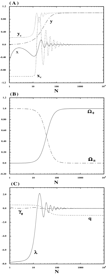
Figure 2: Cosmological dynamics for the field $\phi$ with potential $V(\phi)=V_{0}e^{\frac{1}{2}M^{2}\phi^{2}}$ and a barotropic fluid with $\gamma=1$. The initial conditions are $x_{i}=-0.5$, $y_{i}=6.7\times 10^{-3}$ and $\lambda_{i}=-7.8$. We show the evolution of the same quantities as in Fig. 1.

V Case of $|\lambda|\to\infty$

There are a number of potentials that give $|\lambda|\to\infty$ asymptotically. One can classify the tachyon potentials into two classes: (1) $|\lambda|\to\infty$ without the oscillation of the field $\phi$ [(iiia), (iiib), (iiic)] and (2) $|\lambda|\to\infty$ with the oscillation of the field, that is, $V(\phi)=V_{0}(\phi-\phi_{0})^{n}$ for positive $n$. In the latter case the effective mass squared $m_{\rm eff}^{2}=({\rm log}\,V)_{\phi\phi}$ of the field $\phi$ is negative, which leads to a violent instability for the tachyon perturbations Frolov . This is not regarded as a stable attractor unlike the potential $V(\phi)=V_{0}e^{\frac{1}{2}M^{2}\phi^{2}}$ discussed in the previous section.

We shall investigate the case (1) in which $|\lambda|$ continues to grow asymptotically. For example let us consider the exponential potential $V(\phi)=V_{0}e^{-\mu\phi}$ with $\mu>0$ [case (iiib)]. Since $\Gamma=1$ for this potential, we have $\lambda^{\prime}=(\sqrt{3}/2)\lambda^{2}xy$, thereby leading to the growth of $\lambda$ for $x>0$. In Fig. 3 we plot the cosmological evolution for this system with initial conditions $x_{i}=0.7$, $y_{i}=1.0\times 10^{-4}$ and $\lambda_{i}=0.5$. There is a short initial stage in which the conditions, $x\ll 1$ and $y\ll 1$, are satisfied with $\Omega_{\phi}\simeq 0$ and $\gamma_{\phi}\simeq 0$. This is an unstable fixed point (a) in Table I, thus showing a deviation from $x=0$ and $y=0$ for $N\gtrsim 100$. From the panel (C) we find that the universe begins to accelerate for $N\gtrsim 400$ (see the evolution of $q$). After that $x$ and $y$ approach the instantaneous critical points (c) in Table I. As long as $\lambda\leq{\cal O}(1)$, one can see that the condition $q<0$ is satisfied by substituting $x_{s}=\lambda y_{s}/\sqrt{3}$ and $y=y_{s}$ for Eq. (16). With the growth of $\lambda$, however, the acceleration of the universe stops for $N\gtrsim 6.5\times 10^{4}$. At this stage $x$ grows toward 1, where as $y$ decreases toward 0. The asymptotic behavior corresponds to $x\to 1$ and $y\to\sqrt{3}/\lambda$, which can be obtained by taking the limit $\lambda\gg 1$ for the instantaneous critical points (c) in Table I. Substituting this solution for Eq. (10), we obtain $\lambda\propto e^{3N/2}$. This relation holds when $\Gamma$ is asymptotically constant with $\Gamma>3/2$. In this regime the equation of state for the field $\phi$ is characterized by $\gamma_{\phi}\simeq 1$ (i.e., a pressureless dust) with a dominant energy density ($\Omega_{\phi}\simeq 1$).

It is worth reflecting here briefly on the fact that there exists a period of transient acceleration when we have an exponential potential. Because of a dynamical change of $\lambda$, it is possible to have a temporal acceleration for $\lambda\lesssim 1$ and have a deceleration for $\lambda\gg 1$. If this temporal acceleration corresponds to the one at present, the universe will eventually enter the non-accelerating regime in which the tachyon field behaves as a pressureless dust. This is a nice feature of the model which makes it free from the future event horizon problem present in most of the quintessence models.

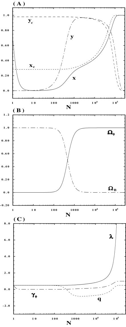
Figure 3: Cosmological evolution for the field $\phi$ with potential $V(\phi)=V_{0}e^{-\mu\phi}$ and the barotropic fluid with $\gamma=1$. Initial conditions are $x_{i}=0.7$, $y_{i}=1.0\times 10^{-4}$ and $\lambda_{i}=0.5$. We show the evolution of the same quantities as in Fig. 1.

As long as $|\lambda|$ approaches infinity asymptotically, we do not have an acceleration of the universe at late times. This comes from the fact that the fixed point (c) in Table I approaches $x\to 1$ and $y\simeq\sqrt{3}/\lambda\to 0$ as $|\lambda|\to\infty$. Therefore any potentials which exhibit this behavior can not be used as a late-time dark energy candidate. In order to lead to acceleration at late times, we require that the tachyon potential has the property (i) $\lambda={\rm const}$ or (ii) $\lambda\to 0$ asymptotically, as we showed in previous sections. Of course, as we have just mentioned, it is possible that the acceleration we are experiencing is not a late time evolution, but part of a transient regime!

VI Summary

In this paper we have studied the cosmology associated with the tachyon field $\phi$ as the dark energy. In the tachyon system the inverse square potential (17) is the marginal case which leads to an accelerating universe. However, it is not the only possible tachyon potential and so we have deliberately set out to develop a unified analysis that can be applied for any type of tachyon potentials.

A crucial quantity to determine the cosmological dynamics is $\lambda$ defined in Eq. (11). The inverse square potential (17) corresponds to a constant $\lambda$ with $\lambda=2M_{p}/M$. In this case we have essentially four critical points as shown in Table I. Among them a viable fixed point that gives a stable attractor for dark energy is the case (c) with a barotropic equation of state $\gamma$ larger than $\gamma_{s}$ [$\gamma_{s}$ is defined in Eq. (30)]. The critical point (d) corresponds to a scaling solution in which the energy density of $\phi$ decreases similarly to that of the barotropic fluid. However this is not a viable cosmological scaling solution, since the existence of it requires the condition $\gamma<1$.

The tachyon potentials can be placed into three classes: (i) $\lambda={\rm const}$, (ii) $\lambda\to 0$ asymptotically and (iii) $|\lambda|\to\infty$ asymptotically. The class (ii) corresponds to the case in which the potential is not steep relative to $V(\phi)=M^{2}\phi^{-2}$, whereas the potential in the class (iii) is steeper than $V(\phi)=M^{2}\phi^{-2}$. While the former leads to the acceleration at late times, the latter does not.

We have carried out a detailed analysis about the cosmological evolution of the tachyon system in two cases: (1) $\lambda\to 0$ without the oscillation of $\phi$ and (2) $\lambda\to 0$ with the oscillation of $\phi$. We adopt the inverse power-law potential $V(\phi)=M^{4-n}\phi^{-n}$ with $0<n<2$ as an example of the case (1). This is favorable relative to the inverse quadratic potential ($n=2$), since the mass scale $M$ is not severely constrained. We solved the dynamical equations (8)-(10) numerically and found that the solutions approach the “instantaneous” critical point (c) in Table I with the decrease of $\lambda$ toward 0 [see the panel (A) of Fig. 1]. Since $x\simeq\lambda(N)/\sqrt{3}\to 0$ and $y\simeq 1-\lambda(N)^{2}/12\to 1$ as $\lambda(N)\to 0$, the universe exhibits an acceleration at late times. This is a dark energy scenario in which the future universe is dominated by the field $\phi$ ($\Omega_{\phi}\simeq 1$) with an equation of state $\gamma_{\phi}\simeq 0$. We adopt the rolling massive scalar potential $V(\phi)=V_{0}e^{\frac{1}{2}M^{2}\phi^{2}}$ to study the case (2) mentioned above. We find that $x$ and $y$ again approach the instantaneous critical point (c) with oscillations. Since the potential has an energy $V_{0}$ at the potential minimum, this eventually leads to an acceleration of the universe even if the scalar field oscillates.

On the other hand we do not find an accelerated expansion at late times when $|\lambda|$ grows towards infinity, since the dynamical critical point (c) approaches $x\to 1$ and $y\to 0$ as $|\lambda|\to\infty$. Nevertheless we found that a transient acceleration can occur in the region where $\lambda(N)$ is smaller than of order unity (see Fig. 3). It is tempting to speculate that this could be the transient regime we are experiencing today, and to try and predict when we expect it to change over again to a matter dominated era. Recall that the supernova data is not actually informing us about the evolution today ($z=0$), rather it tells us that the universe is accelerating at a redshift of order 0.05. Perhaps we are actually back in a matter dominated regime today and just don’t know it yet!

Inspite of the existing features of cosmological dynamics based upon DBI scalars, it may happen that these models lead to the formation of caustics where the second and the higher-order derivatives of the field become singular. We do not know whether caustics are generic prediction of string theory or appear as a result of the derivative truncation leading to the DBI action. As demonstrated in Ref. FKS , caustics inevitably form in tachyon system with potentials decaying as $\phi^{-2}$ or faster at infinity. It remains to extend the analysis of Ref. FKS to the case of potentials such as $V\sim\phi^{-n}$ with $0<n<2$ analysed in our paper. Caustics normally form in systems with pressureless dust which is mimicked by tachyon field with run away potentials. It is therefore quite likely that caustics may not develop in Born-Infeld systems with a ground state at at a finite value of the field. The rolling massive scalar potential $V(\phi)=V_{0}e^{\frac{1}{2}M^{2}\phi^{2}}$ belongs to this category. In our opinion, these are important issues which require further investigations.

Finally we believe it is quite intriguing that the tachyon system provides rich and fruitful cosmological scenarios for dark energy. The classification we have performed in this paper provides a very useful way to find out about the cosmological evolution for any type of tachyon potentials.

References

- (1) V. Sahni and A. A. Starobinsky, Int. J. Mod. Phys. D 9, 373 (2000); T. Padmanabhan, Phys. Rept. 380, 235 (2003).
- (2) S. Kachru, R. Kallosh, A. Linde and S. P. Trivedi, Phys. Rev. D 68, 046005 (2003).
- (3) I. Zlatev, L. M. Wang and P. J. Steinhardt, Phys. Rev. Lett. 82, 896 (1999); P. J. Steinhardt, L. M. Wang and I. Zlatev, Phys. Rev. D 59, 123504 (1999); L. Amendola, Phys. Rev. D 62, 043511 (2000).
- (4) C. Armendariz-Picon, V. Mukhanov and P. J. Steinhardt, Phys. Rev. Lett. 85, 4438 (2000); Phys. Rev. D 63, 103510 (2001); T. Chiba, T. Okabe and M. Yamaguchi, Phys. Rev. D 62, 023511 (2000).
- (5) G. R. Dvali, G. Gabadadze and M. Porrati, Phys. Lett. B 485, 208 (2000); C. Deffayet, G. R. Dvali and G. Gabadadze, Phys. Rev. D 65, 044023 (2002); V. Sahni and Y. Shtanov, JCAP 0311, 014 (2003); S. M. Carroll, V. Duvvuri, M. Trodden and M. S. Turner, Phys. Rev. D 70, 043528 (2004).
- (6) A. Y. Kamenshchik, U. Moschella and V. Pasquier, Phys. Lett. B 511, 265 (2001); N. Bilic, G. B. Tupper and R. D. Viollier, Phys. Lett. B 535, 17 (2002); M. C. Bento, O. Bertolami and A. A. Sen, Phys. Rev. D 66, 043507 (2002).
- (7) A. Sen, JHEP 0204, 048 (2002); JHEP 0207, 065 (2002); Mod. Phys. Lett. A 17, 1797 (2002); arXiv: hep-th/0312153.
- (8) A. Sen, JHEP 9910, 008 (1999); M. R. Garousi, Nucl. Phys. B584, 284 (2000); Nucl. Phys. B 647, 117 (2002); JHEP 0305, 058 (2003); E. A. Bergshoeff, M. de Roo, T. C. de Wit, E. Eyras, S. Panda, JHEP 0005, 009 (2000); J. Kluson, Phys. Rev. D 62, 126003 (2000); D. Kutasov and V. Niarchos, Nucl. Phys. B 666, 56 (2003).
- (9) G. W. Gibbons, Phys. Lett. B 537, 1 (2002); M. Fairbairn and M. H. G. Tytgat, Phys. Lett. B 546, 1 (2002); A. Feinstein, Phys. Rev. D 66, 063511 (2002); S. Mukohyama, Phys. Rev. D 66, 024009 (2002); D. Choudhury, D. Ghoshal, D. P. Jatkar and S. Panda, Phys. Lett. B 544, 231 (2002); G. Shiu and I. Wasserman, Phys. Lett. B 541, 6 (2002); L. Kofman and A. Linde, JHEP 0207, 004 (2002); M. Sami, Mod. Phys. Lett. A 18, 691 (2003); A. Mazumdar, S. Panda and A. Perez-Lorenzana, Nucl. Phys. B 614, 101 (2001); J. c. Hwang and H. Noh, Phys. Rev. D 66, 084009 (2002); Y. S. Piao, R. G. Cai, X. m. Zhang and Y. Z. Zhang, Phys. Rev. D 66, 121301 (2002); J. M. Cline, H. Firouzjahi and P. Martineau, JHEP 0211, 041 (2002); S. Mukohyama, Phys. Rev. D 66, 123512 (2002); M. C. Bento, O. Bertolami and A. A. Sen, Phys. Rev. D 67, 063511 (2003); J. g. Hao and X. z. Li, Phys. Rev. D 66, 087301 (2002); C. j. Kim, H. B. Kim and Y. b. Kim, Phys. Lett. B 552, 111 (2003); T. Matsuda, Phys. Rev. D 67, 083519 (2003); A. Das and A. DeBenedictis, arXiv:gr-qc/0304017; Z. K. Guo, Y. S. Piao, R. G. Cai and Y. Z. Zhang, Phys. Rev. D 68, 043508 (2003); G. W. Gibbons, Class. Quant. Grav. 20, S321 (2003); M. Majumdar and A. C. Davis, arXiv:hep-th/0304226; S. Nojiri and S. D. Odintsov, Phys. Lett. B 571, 1 (2003); E. Elizalde, J. E. Lidsey, S. Nojiri and S. D. Odintsov, Phys. Lett. B 574, 1 (2003); D. A. Steer and F. Vernizzi, Phys. Rev. D 70, 043527 (2004); V. Gorini, A. Y. Kamenshchik, U. Moschella and V. Pasquier, Phys. Rev. D 69, 123512 (2004); L. P. Chimento, Phys. Rev. D 69, 123517 (2004); M. B. Causse, arXiv:astro-ph/0312206; B. C. Paul and M. Sami, Phys. Rev. D 70, 027301 (2004); G. N. Felder and L. Kofman, Phys. Rev. D 70, 046004 (2004); J. M. Aguirregabiria and R. Lazkoz, Mod. Phys. Lett. A 19, 927 (2004); L. R. Abramo, F. Finelli and T. S. Pereira, arXiv:astro-ph/0405041; G. Calcagni, arXiv:hep-th/0406006; J. Raeymaekers, JHEP 0410, 057 (2004); G. Calcagni and S. Tsujikawa, Phys. Rev. D 70, 103514 (2004); S. K. Srivastava, arXiv:gr-qc/0409074; N. Barnaby and J. M. Cline, arXiv:hep-th/0410030.
- (10) T. Padmanabhan, Phys. Rev. D 66, 021301 (2002).
- (11) J. S. Bagla, H. K. Jassal and T. Padmanabhan, Phys. Rev. D 67, 063504 (2003).
- (12) L. R. W. Abramo and F. Finelli, Phys. Lett. B 575 (2003) 165.
- (13) J. M. Aguirregabiria and R. Lazkoz, Phys. Rev. D 69, 123502 (2004).
- (14) Z. K. Guo and Y. Z. Zhang, JCAP 0408, 010 (2004).
- (15) E. J. Copeland, A. R. Liddle and D. Wands, Phys. Rev. D 57, 4686 (1998).
- (16) R. J. van den Hoogen, A. A. Coley and D. Wands, Class. Quant. Grav. 16, 1843 (1999).
- (17) A. P. Billyard, A. A. Coley and R. J. van den Hoogen, Phys. Rev. D 58, 123501 (1998).
- (18) A. R. Liddle and R. J. Scherrer, Phys. Rev. D 59, 023509 (1999).
- (19) A. de la Macorra and G. Piccinelli, Phys. Rev. D 61, 123503 (2000).
- (20) S. C. C. Ng, N. J. Nunes and F. Rosati, Phys. Rev. D 64, 083510 (2001).
- (21) K. i. Maeda, Phys. Rev. D 64, 123525 (2001).
- (22) G. Huey and J. E. Lidsey, Phys. Lett. B 514, 217 (2001).
- (23) S. Mizuno and K. i. Maeda, Phys. Rev. D 64, 123521 (2001).
- (24) S. Mizuno, S. J. Lee and E. J. Copeland, Phys. Rev. D 70, 043525 (2004); E. J. Copeland, S. J. Lee, J. E. Lidsey and S. Mizuno, arXiv:astro-ph/0410110.
- (25) F. Piazza and S. Tsujikawa, JCAP 06, 005 (2004).
- (26) M. Sami, N. Savchenko and A. Toporensky, arXiv: hep-th/0408140.
- (27) S. Tsujikawa and M. Sami, Phys. Lett. B 603, 113 (2004).
- (28) B. Wang, E. Abdalla and R. K. Su, Mod. Phys. Lett. A 18, 31 (2003).
- (29) M. R. Garousi, M. Sami and S. Tsujikawa, Phys. Rev. D 70, 043536 (2004); M. R. Garousi, M. Sami and S. Tsujikawa, Phys. Lett. B to appear [arXiv:hep-th/0405012].
- (30) M. Sami, P. Chingangbam and T. Qureshi, Phys. Rev. D 66, 043530 (2002).
- (31) S. Kachru, R. Kallosh, A. Linde, J. Maldacena, L. McAllister and S. P. Trivedi, JCAP 0310, 013 (2003).
- (32) A. Sen, arXiv:hep-th/9904207.
- (33) A. Sen, Phys. Rev. D 68, 066008 (2003).
- (34) N. Lambert, H. Liu and J. Maldacena, arXiv:hep-th/0303139.
- (35) A. V. Frolov, L. Kofman and A. A. Starobinsky, Phys. Lett. B 545, 8 (2002).
- (36) G. N. Felder, L. Kofman and A. Starobinsky, JHEP 0209, 026 (2002).