Abstract

Massless flows from the coset model $su(2)_{k+1}\otimes su(2)_{k}/su(2)_{2k+1}$ to the minimal model $M_{k+2}$ are studied from the viewpoint of form factors. These flows include in particular the flow from the Tricritical Ising model to the Ising model. By analogy with the magnetization operator in the flow TIM $\to$ IM, we construct all form factors of an operator that flows to $\Phi_{1,2}$ in the IR. We make a numerical estimation of the difference of conformal weights between the UV and the IR thanks to the $\Delta$-sum rule; the results are consistent with the conformal weight of the operator $\Phi_{2,2}$ in the UV. By analogy with the energy operator in the flow TIM $\to$ IM, we construct all form factors of an operator that flows to $\Phi_{2,1}$. We propose to identify the operator in the UV with $\sigma_{1}\Phi_{1,2}$.

PACS: 11.10.-z 11.10.Kk 11.55.Ds

Introduction

In our previous article [1], we considered the construction of the form factors of the trace operator in the massless flows [2] from the UV coset model [3] $su(2)_{k+1}\otimes su(2)_{k}/su(2)_{2k+1}$, with central charge

$$c_{\textrm{\tiny UV}}=\frac{3k(k+1)(2k+5)}{(k+2)(k+3)(2k+3)},$$

to the IR coset $su(2)_{k}\otimes su(2)_{1}/su(2)_{k+1}$. The latter model is the unitary minimal model $M_{k+2}$ with central charge

$$c_{\textrm{\tiny IR}}=\frac{k(k+5)}{(k+2)(k+3)}.$$

The flow is defined in UV by the relevant operator of conformal dimension $\Delta=\bar{\Delta}=1-2/(2k+3)$; it arrives in the IR along the irrelevant operator $T\bar{T}$.
These flows include in particular for $k=1$ the famous massless flow from the Tricritical Ising model to the Ising model. The latter flow was studied by Delfino, Mussardo and Simonetti in [4] using a massless version of the form factor approach, originally developed for the massive case in [5, 6, 7]. For this purpose, the authors of [4] used the scattering data proposed by Al.B. Zamolodchikov in [8]. Let us mention that the notion of massless scattering was first introduced and discussed in this latter paper. In [4], beside the trace operator, some form factors for the magnetization operator and the energy operator were constructed.
In this article we will try to generalize this construction to the whole family of flows introduced above.
We do not intend to repeat here the construction of the form factors in the Sine-Gordon model, and would like to refer the reader to our previous paper [1] for notations and formulae, and to [9, 10] for complementary information on the global formalism.
Let us recall that in the massless case, the dispersion relations read $(p^{0},p^{1})=\frac{M}{2}(e^{\theta},e^{\theta})$ for right movers and $(p^{0},p^{1})=\frac{M}{2}(e^{-\theta^{\prime}},-e^{-\theta^{\prime}})$ for left movers, where $M$ is some mass-scale in the theory, and $\theta,\theta^{\prime}$ the rapidity variables. Zero momentum corresponds to $\theta\to-\infty$ for right movers and $\theta^{\prime}\to+\infty$ for left movers.
The $S$-matrices for the three different scatterings were found in [11]: the $RR$ and $LL$ $S$-matrices describe the IR CFT $M_{k+2}$, and are thus given by the RSOS restriction of the Sine-Gordon $S$-matrix [12, 13].
We introduce by anticipation the minimal form factor in the SG model:

$$f_{p}(\theta)=-\mathrm{i}\sinh\frac{\theta}{2}f^{min}_{p}(\theta)=-\mathrm{i}\sinh\frac{\theta}{2}\exp\int_{0}^{\infty}\frac{dt}{t}\frac{\sinh\frac{1}{2}(1-p)t}{\sinh\frac{1}{2}pt\cosh\frac{1}{2}t}\frac{1-\cosh t(1-\frac{\theta}{\mathrm{i}\pi})}{2\sinh t},$$

where the parameter $p$ is related to the parameter $k$ by $p\equiv k+2$.
As for the $RL$ scattering, it is given by[11]:

$$S_{RL}(\theta-\theta^{\prime})=\frac{1}{S_{LR}(\theta^{\prime}-\theta)}=\tanh\left(\frac{\theta-\theta^{\prime}}{2}-\frac{\mathrm{i}\pi}{4}\right)\,.$$

In the IR limit, the scattering becomes trivial $S_{RL}(\theta-\theta^{\prime})\to-1$, and the two chiralities decouple.
The minimal form-factor in the RL channel satisfies the relation:

$$f_{RL}(\theta-\theta^{\prime})=f_{RL}(\theta-\theta^{\prime}+2\mathrm{i}\pi)S_{RL}(\theta-\theta^{\prime}),$$

and its explicit expression is given by

$$f_{RL}(\theta-\theta^{\prime})=\exp\left(\frac{(\theta-\theta^{\prime}-\mathrm{i}\pi)}{4}-\int_{0}^{+\infty}\;\frac{dt}{t}\frac{1-\cosh t\left(1-\frac{(\theta-\theta^{\prime})}{\mathrm{i}\pi}\right)}{2\sinh t\cosh\frac{t}{2}}\right).$$

Its asymptotic behaviour in the infrared is: $f_{RL}(\theta-\theta^{\prime})\sim\mathcal{K}\;e^{\frac{1}{2}(\theta-\theta^{\prime}-\mathrm{i}\pi)}$, where

$$\mathcal{K}=\exp{-\frac{1}{2}\int_{0}^{\infty}\frac{dt}{t}\left(\frac{1}{\sinh t\cosh\frac{t}{2}}-\frac{1}{t}\right)}.$$

The plan of the paper is the following: in Section 1, we generalize the construction of the form factors of the magnetization operator in the flow TIM $\to$ IM, i.e. we construct form factors of an operator that flows to $\Phi_{1,2}$ in the IR. Then we make numerical checks involving the $\Delta$-sum rule, in order to identify the conformal dimension of the operator in the UV. Section 2 is devoted to the generalization of the form factors of the energy operator in the flow TIM $\to$ IM: we construct form factors of an operator which flows in the IR to the operator $\Phi_{2,1}$ in $M_{k+2}$; an analysis of the two point correlator for such an operator can also be found. Finally, we give some concluding remarks.

1 Form factors of an operator $\Phi$ that flows to $\Phi_{1,2}$ in $M_{p}$.

1.1 Magnetization operator in the flow from TIM to IM.

A few form factors of the magnetization operator were obtained in [4] in terms of symmetric polynomials for the case $k=1$ ($p=3$) corresponding to the massless flow from TIM to IM. Due to the invariance of the theory under spin reversal, the order operator has non vanishing form factors only on a odd number of particles, whereas the disorder operator only on an even one. We shall consider the case of the disorder operator with even number of right and left particles.
We recall that the form factors of this operator satisfy the following residue equation at $\theta_{1}=\theta_{2r}+\mathrm{i}\pi$ [4, 15]:

$$\mathrm{res}F_{2r,2l}(\theta_{1},\cdots,\theta_{2r};\theta^{\prime}_{1},\cdots,\theta^{\prime}_{2l})=-2\mathrm{i}\;F_{2r-2,2l}(\theta_{2},\cdots,\theta_{2r-1};\theta^{\prime}_{1},\cdots,\theta^{\prime}_{2l})\left(1+\prod_{k=1}^{2l}S_{RL}(\theta_{2r}-\theta^{\prime}_{k})\right),$$

and a similar equation in the $LL$ channel. The first step of recursion is given by $F_{0,0}=1$.
In [16] it was observed that all form factors of this operator could be rewritten as:

$$F_{2r,2l}(\theta_{1},\ldots,\theta_{2r};\theta^{\prime}_{1},\ldots,\theta^{\prime}_{2l})=$$

$$\prod_{1\leq i<j\leq 2r}\sinh\frac{\theta_{ij}}{2}\prod_{1\leq i<j\leq 2l}\sinh\frac{\theta^{\prime}_{ij}}{2}\prod_{i,j}f_{RL}(\theta_{i}-\theta^{\prime}_{j})Q_{2r,2l}(\theta_{1},\ldots,\theta_{2r};\theta^{\prime}_{1},\ldots,\theta^{\prime}_{2l}),$$

where

$$Q_{2r,2l}(\theta_{1},\ldots,\theta_{2r};\theta^{\prime}_{1},\ldots,\theta^{\prime}_{2l})=$$

$$(-\mathrm{i}\pi)^{r+l}\sum_{T\subset S,\atop\#T=r}\sum_{T^{\prime}\subset S^{\prime},\atop\#T^{\prime}=l}\prod_{i\in T,\atop k\in\bar{T}}\phi(\theta_{ik})e^{\frac{1}{2}\sum\theta_{ki}}\prod_{i\in T^{\prime},\atop k\in\bar{T}^{\prime}}\phi(\theta^{\prime}_{ik})e^{\frac{1}{2}\sum\theta^{\prime}_{ik}}\prod_{i\in T,\atop k\in\bar{T}^{\prime}}\Phi(\theta_{i}-\theta^{\prime}_{k})\prod_{i\in T^{\prime},\atop k\in\bar{T}}\tilde{\Phi}(\theta_{k}-\theta^{\prime}_{i}),$$

and

$$\phi(\theta_{ij})\equiv\frac{-1}{f_{RR}(\theta_{ij})f_{RR}(\theta_{ij}+\mathrm{i}\pi)}=\frac{2\mathrm{i}}{\sinh\theta_{ij}}\;,\quad\phi(\theta^{\prime}_{ij})\equiv\frac{-1}{f_{LL}(\theta^{\prime}_{ij})f_{LL}(\theta^{\prime}_{ij}+\mathrm{i}\pi)}=\frac{2\mathrm{i}}{\sinh\theta^{\prime}_{ij}}\;,$$ (1)

as well as:

$$\Phi(\theta-\theta^{\prime})\equiv\frac{S_{RL}(\theta-\theta^{\prime})}{f_{RL}(\theta-\theta^{\prime})f_{RL}(\theta-\theta^{\prime}+\mathrm{i}\pi)}=\mathcal{K}^{-2}(1-\mathrm{i}e^{\theta^{\prime}-\theta}),\quad\tilde{\Phi}(\theta-\theta^{\prime})\equiv\Phi(\theta-\theta^{\prime}+\mathrm{i}\pi).$$ (2)

It was found in [4] that for two right and two left particles, the expression of the form factor is given by the following expression:

$$F_{2,2}(\theta_{1},\theta_{2};\theta^{\prime}_{1},\theta^{\prime}_{2})=\frac{1}{4\mathcal{K}^{4}}\tanh\frac{\theta_{12}}{2}\tanh\frac{\theta^{\prime}_{12}}{2}\prod_{i=1,2\atop j=1,2}f_{RL}(\theta_{i}-\theta^{\prime}_{j})\;(1+e^{\theta^{\prime}_{1}+\theta^{\prime}_{2}-\theta_{1}-\theta_{2}}).$$ (3)

The following relation holds when $\theta_{i}-\theta^{\prime}_{j}\to-\infty$ which defines the IR region [4, 16]:

$$F_{2r,2l}(\theta_{1},\ldots,\theta_{2r};\theta^{\prime}_{1},\ldots,\theta^{\prime}_{2l})\to F_{2r}^{\mu}(\theta_{1},\ldots,\theta_{2r})F_{2l}^{\mu}(\theta^{\prime}_{1},\ldots,\theta^{\prime}_{2l}),$$

where $F_{2r}^{\mu}(\theta_{1},\ldots,\theta_{2r})$ are the form factors of the disorder operator $\mu=\Phi_{1,2}$ in the thermal Ising model [6, 15, 17]:

$$F_{2r}^{\mu}(\theta_{1},\ldots,\theta_{2r})=\frac{1}{2^{r(2r-1)}}\prod_{1\leq i<j<\leq 2r}\tanh\frac{\theta_{ij}}{2}.$$

1.2 Generalization

By analogy with the previous section, we shall now look for a solution to the following problem at $\theta_{1}=\theta_{2r}+\mathrm{i}\pi$:

$$\mathrm{res}F_{2r,2l}^{\Phi}(\theta_{1},\cdots,\theta_{2r};\theta^{\prime}_{1},\cdots,\theta^{\prime}_{2l})=$$

$$-2\mathrm{i}\;F_{2r-2,2l}^{\Phi}(\theta_{2},\cdots,\theta_{2r-1};\theta^{\prime}_{1},\cdots,\theta^{\prime}_{2l})\left(1+\prod_{i=2}^{2r-1}S^{RSOS}_{p}(\theta_{i}-\theta_{2r})\prod_{k=1}^{2l}S_{RL}(\theta_{2r}-\theta^{\prime}_{k})\right)e^{R},$$

where $e^{R}=e^{\frac{\mathrm{i}\pi}{2p}}s_{1}\otimes\bar{s}_{2r}+e^{-\frac{\mathrm{i}\pi}{2p}}\bar{s}_{1}\otimes s_{2r}$. A similar equation holds in the $LL$ channel.
Let us note that in the IR limit, given that $S_{RL}\to-1$, the latter relation becomes

$$\mathrm{res}F_{2r,2l}^{\Phi}(\theta_{1},\cdots,\theta_{2r};\theta^{\prime}_{1},\cdots,\theta^{\prime}_{2l})=$$

$$-2\mathrm{i}\;F_{2r-2,2l}^{\Phi}(\theta_{2},\cdots,\theta_{2r-1};\theta^{\prime}_{1},\cdots,\theta^{\prime}_{2l})\left(1+\prod_{i=2}^{2r-1}S^{RSOS}_{p}(\theta_{i}-\theta_{2r})\right)e^{R},$$

which is the residue equation satisfied by (amongst others) the operator $\Phi_{1,2}$ in $M_{p}$.
We construct a solution to the residue equation (1.2) with the initial condition $F_{0,0}^{\Phi}=\langle\Phi\rangle$, and with the following condition in the IR limit:

$$F_{2r,2l}^{\Phi}(\theta_{1},\cdots,\theta_{2r};\theta^{\prime}_{1},\cdots,\theta^{\prime}_{2l})\to\langle\Phi\rangle\;f_{RSOS}^{\Phi_{1,2}}(\theta_{1},\cdots,\theta_{2r})\;f_{RSOS}^{\Phi_{1,2}}(\theta^{\prime}_{1},\cdots,\theta^{\prime}_{2l}).$$ (5)

In other words, we want to construct form factors of an operator that renormalizes in the IR on the operator $\Phi_{1,2}$ in $M_{p}$.
We make the following ansatz for the solution, to be compared with the one obtained for the trace operator in [1] (once again, we refer the reader to [1, 9, 10] for further explanations on the construction of form factors in the SG model and basic notations):

$$F_{2r,2l}^{\Phi}(\theta_{1},\dots,\theta_{2r};\theta^{\prime}_{1},\dots,\theta^{\prime}_{2l})=\langle\Phi\rangle N^{\Phi}_{2r}N^{\Phi}_{2l}\prod_{1\leq i<j\leq 2r}f_{p}(\theta_{ij})\prod_{1\leq i<j\leq 2l}f_{p}(\theta^{\prime}_{ij})\prod_{i,j}f_{RL}(\theta_{i}-\theta^{\prime}_{j})$$ (6)

$$\times\int_{C_{\theta}}\prod_{m=1}^{r}du_{m}\;h_{RR}(\theta,u)p^{\frac{1}{2}}_{2r}(\theta,u)\tilde{\Psi}^{p}(\theta,{u})\;\int_{C_{\theta^{\prime}}}\prod_{m=1}^{l}dv_{m}\;h_{LL}(\theta^{\prime},v)p^{\frac{1}{2}}_{2l}(\theta^{\prime},v)\tilde{\Psi}^{p}(\theta^{\prime},{v})$$

$$\times\;\mathcal{N}_{2r,2l}(\theta,\theta^{\prime},{u},{v}).$$

We introduced $p^{\frac{1}{2}}(\theta,u)$, which is the $p$-function of the operator $\Phi_{1,2}$ in the minimal model $M_{p}$. We use the identification $\Phi_{1,2}\sim e^{\mathrm{i}\frac{\beta}{2}\varphi_{SG}}$, followed by a modification of the multiparticles state [13]: the modified Bethe ansatz state $\tilde{\Psi}^{p}$ is related to the usual Bethe ansatz state by the relation [13]

$$\tilde{\Psi}^{p}_{\epsilon_{1}\epsilon_{2}\dots\epsilon_{2n}}(\theta,u)\equiv e^{\frac{1}{2p}\sum_{i}\epsilon_{i}\theta_{i}}\Psi^{p}_{\epsilon_{1}\epsilon_{2}\dots\epsilon_{2n}}(\theta,u),\quad\epsilon_{i}=\pm,\;\sum_{i=1}^{2n}\epsilon_{i}=0.$$

We will use the $p$-function of the exponential fields $e^{\mathrm{i}\alpha\varphi}$ in the SG model for the particular value $\alpha=\beta/2$ (the form factors of $e^{\mathrm{i}\alpha\varphi}$ were first constructed in [18]; we use here the conventions and notations of [19]):

$$p^{\frac{1}{2}}_{2n}(\theta,u)=\frac{1}{e^{\frac{\mathrm{i}\pi}{2}}}\frac{\prod_{j=1}^{n}e^{u_{j}}}{\prod_{i=1}^{2n}e^{\frac{\theta_{i}}{2}}}.$$

We introduced the scalar function (completely determined by the $S$-matrix)

$$h_{p}(\theta,u)=\prod_{i=1}^{2n}\prod_{j=1}^{m}\phi_{p}(\theta_{i}-u_{j})\prod_{1\leq r<s\leq m}\tau_{p}(u_{r}-u_{s}),$$

with

$$\phi_{p}(u)=\frac{1}{f_{p}(u)f_{p}(u+\mathrm{i}\pi)},\quad\tau_{p}(u)=\frac{1}{\phi_{p}(u)\phi_{p}(-u)},$$

and $N^{\Phi}_{2r},N^{\Phi}_{2l}$ are normalization constants.
Finally, the integration contours $C_{\theta}$ consist of several pieces for all integration variables $u_{j}$ : a line from $-\infty$ to $\infty$ avoiding all poles such that $\mathrm{Im}\theta_{i}-\pi-\epsilon<\mathrm{Im}u_{j}<\mathrm{Im}\theta_{i}-\pi,$ and clockwise oriented circles around the poles (of the $\phi(\theta_{i}-u_{j})$) at $\theta_{i}=u_{j}$, $(j=1,\dots,m)$. The integration contours $C_{\theta^{\prime}}$ are similarly defined. The function $\mathcal{N}_{2r,2l}$ remains to be determined.
Let us motivate our ansatz (6): it is a slight modification of the results of [9, 10] that the form factors of the operator $\Phi_{1,2}$ in the minimal model $M_{p}$ are written:

$$f_{RSOS}^{\Phi_{1,2}}(\theta_{1},\cdots,\theta_{2r})=N^{\Phi}_{2r}\prod_{1\leq i<j\leq 2r}f_{p}(\theta_{ij})\int_{C_{\theta}}\prod_{m=1}^{r}du_{m}\;h_{RR}(\theta,u)p^{\frac{1}{2}}_{2r}(\theta,u)\tilde{\Psi}^{p}(\theta,{u}).$$

When $\theta_{1}=\theta_{2r}+\mathrm{i}\pi$, each of the $r$ integration contours gets pinched at $\theta_{2r},\theta_{2r}\pm\mathrm{i}\pi$, and we have to take the sum of these three contributions. Due to symmetry, it is enough to consider the contribution of one of them (e.g. $u_{r}$), and multiply the result by $r$. The following computation is detailed in [9]:
at $u_{r}=\theta_{2r}$, we have:

$$\mathrm{res}f_{RSOS}^{\Phi_{1,2}}(\theta_{1},\cdots,\theta_{2r})=-2\mathrm{i}\;f_{RSOS}^{\Phi_{1,2}}(\theta_{2},\cdots,\theta_{2r-1})e^{R},$$

whereas at $u_{r}=\theta_{2r}+\mathrm{i}\pi$:

$$\mathrm{res}f_{RSOS}^{\Phi_{1,2}}(\theta_{1},\cdots,\theta_{2r})=$$

$$-2\mathrm{i}\;f_{RSOS}^{\Phi_{1,2}}(\theta_{2},\cdots,\theta_{2r-1})\prod_{i=2}^{2r-1}S^{RSOS}_{p}(\theta_{i}-\theta_{2r})(e^{\frac{\mathrm{i}\pi}{2p}}s_{1}\otimes\bar{s}_{2r}),$$

and at $u_{r}=\theta_{2r}-\mathrm{i}\pi$:

$$\mathrm{res}f_{RSOS}^{\Phi_{1,2}}(\theta_{1},\cdots,\theta_{2r})=$$

$$-2\mathrm{i}\;f_{RSOS}^{\Phi_{1,2}}(\theta_{2},\cdots,\theta_{2r-1})\prod_{i=2}^{2r-1}S^{RSOS}_{p}(\theta_{i}-\theta_{2r})(e^{-\frac{\mathrm{i}\pi}{2p}}\bar{s}_{1}\otimes s_{2r}).$$

Remembering the relation:

$$f_{RL}(\theta-\theta^{\prime})f_{RL}(\theta-\theta^{\prime}+\mathrm{i}\pi)=\frac{\mathcal{K}^{2}}{1+\mathrm{i}e^{\theta^{\prime}-\theta}},$$

we see that the ansatz (6) will satisfy the residue equation (1.2) at the condition that the function $\mathcal{N}_{2r,2l}(\theta,\theta^{\prime},{u},{v})$ satisfies at $\theta_{1}=\theta_{2r}+\mathrm{i}\pi$:

• $u_{r}=\theta_{2r}$:

  $$\mathcal{N}_{2r,2l}(\theta_{1},\dots,\theta_{2r};\theta^{\prime};u_{1},\dots,u_{r};v)=$$ (7)

  $$\mathcal{N}_{2r-2,2l}(\theta_{2},\dots,\theta_{2r-1};\theta^{\prime};u_{1},\dots,u_{r-1};v)\prod_{k=1}^{2l}\tilde{\Phi}(\theta_{2r}-\theta^{\prime}_{k}).$$

• $u_{r}=\theta_{2r}\pm\mathrm{i}\pi$:

  $$\mathcal{N}_{2r,2l}(\theta_{1}\dots\theta_{2r};\theta^{\prime};u_{1}\dots u_{r};v)=$$ (8)

  $$\mathcal{N}_{2r-2,2l}(\theta_{2},\dots,\theta_{2r-1};\theta^{\prime};u_{1},\dots,u_{r-1};v)\prod_{k=1}^{2l}{\Phi}(\theta_{2r}-\theta^{\prime}_{k}),$$

  and similar relations in the $LL$ channel.

We introduce the sets $S=(1,\dots,2r)$ and $S^{\prime}=(1,\dots,2l)$, as well as $T,U,V$ the subsets of $S$, such that

$$S=T\cup U\cup V,$$

with $T\cap U=\emptyset$ and $V=S-(T\cup V)$. These subsets have number of elements: $\#T=r-1$, $\#U=1$, $\#V=r$.

$$T=\{i_{1}<i_{2}<\dots<i_{r-1}\},\quad U=\{i_{u}\},\quad V=\{k_{1}<k_{2}<\dots<k_{r}\}.$$

The subsets of $S^{\prime}$: $T^{\prime},U^{\prime}$ and $V^{\prime}$ are defined similarly.
We conjecture the following expression:

$$\mathcal{N}_{2r,2l}(\theta,\theta^{\prime},{u},{v})=\frac{1}{\sum_{i=1}^{2r}e^{\theta_{i}}\sum_{i=1}^{2l}e^{-\theta^{\prime}_{i}}}\times\quad\sum_{T\subset S}\sum_{U\subset S}\sum_{T^{\prime}\subset S^{\prime}}\sum_{U^{\prime}\subset S^{\prime}}$$

$$\times\;\frac{\prod_{k,l\in V\atop k<l}\cos\frac{\theta_{kl}}{2\mathrm{i}}\prod_{k\in V}\cos\frac{\theta_{ku}}{2\mathrm{i}}\prod_{i\in T}\cos\frac{\theta_{iu}}{2\mathrm{i}}}{\prod_{i\in T,\atop k\in V}\sin\frac{\theta_{ik}}{2\mathrm{i}}\prod_{i\in T}\sin\frac{\theta_{ui}}{2\mathrm{i}}\prod_{k\in V}\sin\frac{\theta_{ku}}{2\mathrm{i}}}e^{\theta_{u}}\;\frac{\prod_{k,l\in V^{\prime}\atop k<l}\cos\frac{\theta^{\prime}_{kl}}{2\mathrm{i}}\prod_{k\in V^{\prime}}\cos\frac{\theta^{\prime}_{ku}}{2\mathrm{i}}\prod_{i\in T^{\prime}}\cos\frac{\theta^{\prime}_{iu}}{2\mathrm{i}}}{\prod_{i\in T^{\prime},\atop k\in V^{\prime}}\sin\frac{\theta^{\prime}_{ik}}{2\mathrm{i}}\prod_{i\in T^{\prime}}\sin\frac{\theta^{\prime}_{ui}}{2\mathrm{i}}\prod_{k\in V^{\prime}}\sin\frac{\theta^{\prime}_{ku}}{2\mathrm{i}}}e^{-\theta^{\prime}_{u}}$$

$$\times\;\frac{\prod_{i\in T,\atop m=1,\dots,r}\cos\frac{\theta_{i}-u_{m}}{2\mathrm{i}}\prod_{i\in T^{\prime},\atop m=1,\dots,l}\cos\frac{\theta^{\prime}_{i}-v_{m}}{2\mathrm{i}}}{\prod_{1\leq m<n\leq r}\cos\frac{u_{m}-u_{n}}{2\mathrm{i}}\prod_{1\leq m<n\leq l}\cos\frac{v_{m}-v_{n}}{2\mathrm{i}}}\prod_{i\in T\cup U,\atop k\in V^{\prime}}\tilde{\Phi}(\theta_{i}-\theta^{\prime}_{k})\prod_{i\in T^{\prime}\cup U^{\prime},\atop k\in V}\Phi(\theta_{k}-\theta^{\prime}_{i})\;.$$

Let us give a sketch of the proof that this function satisfies the relations (7) and (8):

• when $\theta_{1}=\theta_{2r}+\mathrm{i}\pi$ and $u_{r}=\theta_{2r}$, we cannot have $\theta_{1}\in T$, otherwise the term $\cos\frac{\theta_{1}-u_{r}}{2\mathrm{i}}$ becomes equal to zero. Consequently we should have $\theta_{1}\in U$ or $\theta_{1}\in V$. It follows from a simple inspection of the other cosines in the numerator that the only possibility in order to have the function $\mathcal{N}$ different from zero is to have $\theta_{1}\in V$ and $\theta_{2r}\in T$. Equation (7) follows from the use of simple trigonometric identities.

• conversely, when $\theta_{1}=\theta_{2r}+\mathrm{i}\pi$ and $u_{r}=\theta_{2r}\pm\mathrm{i}\pi$, we find that we should have $\theta_{1}\in T$ and $\theta_{2r}\in V$. Equation (8) follows.

Moreover, it was checked with Mathematica (for a small number of particles) that the relation (5) holds.

1.3 Numerical results

By analogy with what was done in [20] for the flow TIM $\to$ IM, one can think of using the $\Delta$-sum rule in order to compute the variation of the conformal dimension and hence identify the conformal dimension of the operator in the UV. We recall the relation [20]:

$$D\equiv\Delta^{\textrm{\tiny UV}}_{\Phi}-\Delta^{\textrm{\tiny IR}}_{\Phi}=-\frac{1}{2\langle\Phi\rangle}\int_{0}^{\infty}dr\;r\;\langle\Theta(r)\Phi(0)\rangle,$$ (9)

where $\langle\Phi\rangle$ is the vacuum expectation value of the operator $\Phi$, and $\Theta$ the trace operator.
For our purpose, we will need the expression of the 4-particles form factor of $\Theta$ found in [1]:

$$F^{\Theta}(\theta_{1},\theta_{2};\theta^{\prime}_{1},\theta^{\prime}_{2})$$

$$=\frac{16\pi M^{2}}{p^{2}\mathcal{K}^{4}}\;f_{p}(\theta_{12})f_{p}(\theta^{\prime}_{12})\prod_{i=1,2\atop j=1,2}f_{RL}(\theta_{i}-\theta^{\prime}_{j})\;\frac{\cosh\frac{\theta_{12}}{2}\cosh\frac{\theta^{\prime}_{12}}{2}\;e^{R}\otimes e^{L}}{\sinh\frac{1}{p}(\mathrm{i}\pi-\theta_{12})\sinh\frac{1}{p}(\mathrm{i}\pi-\theta^{\prime}_{12})},$$

as well as the 4-particles form factor of the operator $\Phi$. The formula presented in the previous section considerably simplifies for 4 particles:

$$\mathcal{N}_{2,2}(\theta_{1},\theta_{2};\theta^{\prime}_{1},\theta^{\prime}_{2};u,v)=\mathcal{K}^{-4}(1+e^{\theta^{\prime}_{1}+\theta^{\prime}_{2}-\theta_{1}-\theta_{2}}),$$

and this leads to the following expression for the form factor:

$$F^{\Phi}(\theta_{1},\theta_{2};\theta^{\prime}_{1},\theta^{\prime}_{2})$$ (10)

$$=\frac{\langle\Phi\rangle}{p^{2}\mathcal{K}^{4}}f_{p}(\theta_{12})f_{p}(\theta^{\prime}_{12})\prod_{i=1,2\atop j=1,2}f_{RL}(\theta_{i}-\theta^{\prime}_{j})\;\frac{(1+e^{\theta^{\prime}_{1}+\theta^{\prime}_{2}-\theta_{1}-\theta_{2}})\;e^{R}\otimes e^{L}}{\sinh\frac{1}{p}(\mathrm{i}\pi-\theta_{12})\sinh\frac{1}{p}(\mathrm{i}\pi-\theta^{\prime}_{12})}.$$

The normalization of the latter form factor was chosen in order to ensure the initial condition $F^{\Phi}_{0,0}=\langle\Phi\rangle$. This amounts to setting the constant: $N^{\Phi}_{2}=\frac{\mathcal{C}^{4}_{p}}{\pi p}$ in formula (6), where $\mathcal{C}^{4}_{p}$ is defined by the asymptotic behaviour when $\theta\to\pm\infty$ of the minimal form factor:

$$f_{p}(\theta)\sim\mathcal{C}_{p}\;e^{\pm\frac{1}{4}(\frac{1}{p}+1)(\theta-\mathrm{i}\pi)}.$$

Explicitly:

$$\mathcal{C}_{p}=\frac{1}{2}\exp\frac{1}{2}\int_{0}^{\infty}\frac{dt}{t}\left(\frac{\sinh\frac{1}{2}(1-p)t}{\sinh\frac{1}{2}pt\cosh\frac{1}{2}t\sinh t}-\frac{1-p}{pt}\right).$$

The four particle form factor (10) at $p=3$ should be compared with equation (3); in this case we have:

$$\frac{f_{3}(\theta_{12})}{\sinh\frac{1}{3}(\mathrm{i}\pi-\theta_{12})}=-\frac{3}{2}\tanh\frac{\theta_{12}}{2},$$

and consequently the two expressions are identical.
For an arbitrary number of particles, our general construction (6) for $p=3$ should reduce to the formula presented in section 1.1. This looks quite a non trivial task to be performed, and we hope we can return to this issue in the future (a similar situation has already occured in [1] and [19]).
Let us note finally that the v.e.v $\langle\Phi\rangle$ does not need to be known exactly, as it does not enter the numerical estimation.
In order to apply the $\Delta$-sum rule test, it is important to have in mind a UV operator that could be a good candidate: we recall that the numerical tests on the central charge in [1] already showed quite a large discrepancy with respect to the exact results, so we do not expect the sum rule for the conformal dimension to give particularly accurate results.
The minimal model $M_{k+2}$ is nothing but the coset model $su(2)_{k}\otimes su(2)_{1}/su(2)_{k+1}$, and we will denote the latter $\mathcal{M}(k+2,3)$. The operator $\Phi_{1,2}$ in $\mathcal{M}(k+2,3)$ has conformal dimension

$$\Delta_{1,2}^{\textrm{\tiny{IR}}}=\frac{k}{4(k+3)},$$

which is the same as $\Phi_{2,2}$ in the coset model $\mathcal{M}(3,k+2)$. From the perturbative RG calculations [22, 21] for the $\Phi_{1,3}$ induced flow from $M_{k+3}$ to $M_{k+2}$, and the Landau-Ginzburg representation [22, 23], it is well known that one expects $\Phi_{2,2}$ in $M_{k+3}$ to flow to $\Phi_{2,2}$ in $M_{k+2}$ for $k$ odd. For $k=1$, $\Phi_{2,2}$ in $M_{4}$ has conformal dimension $\frac{3}{80}$, and $\Phi_{2,2}=\Phi_{1,2}$ in $M_{3}$ has conformal dimension $\frac{1}{16}$. This flow was later confirmed by [24] by guessing massless TBA equations for the first excited state in the theory $M_{4}$, via a suitable modification of the massless TBA equations for the ground state found in [8].
Then, using the form factors obtained in [4] for the flow TIM $\to$ IM, the authors of [20] successfully identified the conformal dimension of $\Phi_{2,2}$ in the UV thanks to the $\Delta$-sum rule.
Some results are also available about the massless flows between N=1 unitary superconformal models, thanks to perturbative RG analysis [25]. In particular, the results obtained in this article indicate that (at least for $l$ large), there exist flows $\Phi_{2,2}\to\Phi_{2,2}$ from $\mathcal{M}(l+3,4)$ to $\mathcal{M}(l+1,4)$, (the case we are particularly interested in is given by $l=2$, which is not covered by RG analysis).
Consequently, we find it natural enough -let us recall that the operator $\Phi_{2,2}$ in the coset $\mathcal{M}(m,k+2)$, which conformal weight is $\Delta_{2,2}=\frac{3k}{4m(m+k)}$, is the fundamental Landau-Ginzburg field-  to conjecture that we are dealing with $\Phi\equiv\Phi_{2,2}$ in $\mathcal{M}(k+3,k+2)$, flowing to $\Phi_{2,2}$ in $\mathcal{M}(3,k+2)$. The conformal dimension of the UV operator $\Phi_{2,2}$ is:

$$\Delta_{2,2}^{\textrm{{\tiny UV}}}=\frac{3k}{4(k+3)(2k+3)},$$

and we conjecture that the variation of the conformal dimension along the flow is given by:

$$D_{k}^{\textrm{\tiny exact}}=\Delta_{2,2}^{\textrm{{\tiny UV}}}-\Delta_{2,2}^{\textrm{{\tiny IR}}}=\Delta_{2,2}^{\textrm{{\tiny UV}}}-\Delta_{1,2}^{\textrm{{\tiny IR}}}=-\frac{k^{2}}{2(k+3)(2k+3)}.$$

In Table 1 we present the numerical estimation versus the exact result: we find a good agreement between them, at least within the precision of the four-particle approximation (the discrepancies given in the last column of Table 1 are compatible with such an approximation). Let us note also that the accuracy of the results observed here is actually better than the one we had obtained for the $c$-theorem in [1], where it had appeared that the precision of the numerical results diminished as one increased $k$. In our previous paper, we had linked this phenomenon to the fact that the conformal weight of the trace operator

$$\Delta^{\Theta}=\bar{\Delta}^{\Theta}=1-\frac{2}{2k+3},$$

gets closer to one as $k$ increases, spoiling thus the convergence in the UV of the integral expressing the variation of the central charge.

The funny pattern observed in Table 1 is a bit more difficult to explain; we believe it could be caused by a combined effect of $\Delta^{\Theta}\to 1$ when $k\to\infty$, as well as the non monotonic behaviour of $\Delta^{\textrm{{\tiny UV}}}_{2,2}$, as $\Delta^{\textrm{{\tiny UV}}}_{2,2}\to 0$ for both $k\to 0$ and $k\to\infty$.

In any case, we have little doubt that the $\Delta$-sum rule supports our conjecture. Still, it would be interesting to confirm our result by means of other methods (we have in mind the TBA analysis, in a similar way to what has been done in [24]).

$k$	$D_{k}^{\textrm{\tiny num}}$	$D_{k}^{\textrm{\tiny exact}}$	% dev.	$\Delta_{2,2}^{\textrm{{\tiny UV}}}$	$\Delta^{\Theta}$
$1$	$-0.0254(2)$	$-0.025$	$1.6\%$	$0.0375$	$0.6$
$2$	$-0.0609(3)$	$-0.057142\dots$	$6.6\%$	$0.042857\dots$	$0.714286\dots$
$3$	$-0.0910(3)$	$-0.083333\dots$	$9.2\%$	$0.041666\dots$	$0.777777\dots$
$4$	$-0.1152(5)$	$-0.103896\dots$	$10.9\%$	$0.038961\dots$	$0.818181\dots$
$6$	$-0.151(2)$	$-0.133333\dots$	$13.2\%$	$0.033333\dots$	$0.866666\dots$
$10$	$-0.189(1)$	$-0.167224\dots$	$13.0\%$	$0.025083\dots$	$0.913043\dots$
$20$	$-0.220(1)$	$-0.202224\dots$	$8.8\%$	$0.015166\dots$	$0.953488\dots$
$50$	$-0.242(2)$	$-0.228979\dots$	$5.7\%$	$0.006869\dots$	$0.980583\dots$
$100$	$-0.246(2)$	$-0.239131\dots$	$3.0\%$	$0.003586\dots$	$0.990148\dots$
$\infty$	$-0.251(1)$	$-0.25$	$0.8\%$	$0$	$1$

Table 1: Four particle approximation - comparison between $D_{k}^{\textrm{\tiny num}}$ and $D_{k}^{\textrm{\tiny exact}}$ (conjectured variation of the conformal dimension).

2 Form factors of an operator $\Psi$ that flows to the chiral components of $\Phi_{2,1}$ in the $M_{p}$ model.

2.1 Energy operator in the flow between TIM and IM.

We recall that for the massless flow between TIM and IM, the asymptotic states consist of right and left Majorana fermions, with Lorentz spin $\mathrm{s}=\pm 1/2$. The form factors of the energy operator $\epsilon$ have non zero matrix elements for an odd number of right particles and an odd number of left particles. They satisfy the residue equation in the $RR$ channel at $\theta_{1}=\theta_{2r+1}+\mathrm{i}\pi$ (we recall that $S_{RR}=S_{LL}=-1$):

$$\mathrm{res}F^{\epsilon}_{2r+1,2l+1}(\theta_{1},\cdots,\theta_{2r+1};\theta^{\prime}_{1},\cdots,\theta^{\prime}_{2l+1})$$

$$=-2\mathrm{i}\;F^{\epsilon}_{2r-1,2l+1}(\theta_{2},\cdots,\theta_{2r};\theta^{\prime}_{1},\cdots,\theta^{\prime}_{2l+1})\left(1-(-1)^{2r-1}\prod_{k=1}^{2l+1}S_{RL}(\theta_{2r+1}-\theta^{\prime}_{k})\right)$$

and a similar relation in the $LL$ channel. It was noticed in [16] that they could be written as:

$$F_{2r+1,2l+1}^{\epsilon}(\theta_{1},\ldots,\theta_{2r+1};\theta^{\prime}_{1},\ldots,\theta^{\prime}_{2l+1})=\frac{\mathrm{i}M}{\mathcal{K}}\prod_{1\leq i<j\leq 2r+1}\sinh\frac{\theta_{ij}}{2}\prod_{1\leq i<j\leq 2l+1}\sinh\frac{\theta^{\prime}_{ij}}{2}$$

$$\times\;\prod_{i,j}f_{RL}(\theta_{i}-\theta^{\prime}_{j})\;Q_{2r+1,2l+1}^{\epsilon}(\theta_{1},\ldots,\theta_{2r+1};\theta^{\prime}_{1},\ldots,\theta^{\prime}_{2l+1}).$$

The expression for $Q_{2r+1,2l+1}^{\epsilon}$ being given by:

$$Q^{\epsilon}_{2r+1,2l+1}(\theta_{1},\ldots,\theta_{2r+1};\theta^{\prime}_{1},\ldots,\theta^{\prime}_{2l+1})=$$

$$\pi^{r+l}\sum_{T\subset S,\atop\#T=r}\sum_{T^{\prime}\subset S^{\prime},\atop\#T^{\prime}=l}\prod_{i\in T,\atop k\in\bar{T}}\phi(\theta_{ik})\prod_{i\in T^{\prime},\atop k\in\bar{T}^{\prime}}\phi(\theta^{\prime}_{ik})\prod_{i\in T,\atop k\in\bar{T}^{\prime}}\Phi(\theta_{i}-\theta^{\prime}_{k})\prod_{i\in T^{\prime},\atop k\in\bar{T}}\tilde{\Phi}(\theta_{k}-\theta^{\prime}_{i}),$$

where the functions $\phi(\theta)$ and $\Phi(\theta)$ are defined in (1) and (2) above, and the first recursion step is [4]:

$$F_{1,1}^{\epsilon}(\theta_{1};\theta^{\prime}_{1})=\frac{\mathrm{i}M}{\mathcal{K}}f_{RL}(\theta_{1}-\theta^{\prime}_{1}).$$

In the IR, $F_{1,1}^{\epsilon}(\theta_{1};\theta^{\prime}_{1})\to Me^{\frac{1}{2}(\theta-\theta^{\prime})}\sim\psi\bar{\psi}\sim\epsilon_{\mathrm{Ising}}$, with conformal dimension $\Delta_{\textrm{\tiny IR}}=\bar{\Delta}_{\textrm{\tiny IR}}=1/2$. The authors of [4] checked numerically that the power law behaviour in the UV of the two point correlation function truncated to one right and one left particle agreed with the expected conformal dimension $(1/10,1/10)$ of the field $\Phi_{1,2}$ in TIM.

2.2 Generalizations

We generalize the previous results for any value of $p$: the important observation is that the primary field $\Phi_{2,1}$ in $M_{p}$ has conformal dimension $\Delta_{2,1}=\bar{\Delta}_{2,1}=\frac{1}{4}+\frac{3}{4p}$: for $p=3$ it is nothing but the energy operator $\epsilon=\bar{\psi}\psi$ in the Ising model, and for $p=+\infty$, it coincides with the spinon field of the $SU(2)_{1}$ WZNW model. It is thus natural to think of each chiral components as a generalized fermion for $p$ arbitrary (in other words, its chiral components generate the asymptotic states) [26].
We call $g_{\uparrow\downarrow}$ and $\bar{g}_{\uparrow\downarrow}$ the holomorphic components of $\Phi_{2,1}$: $g_{\uparrow}$,$\;\bar{g}_{\uparrow}$ have Lorentz spin $\Delta_{2,1}$, whereas $g_{\downarrow}$,$\;\bar{g}_{\downarrow}$ have Lorentz spin $-\Delta_{2,1}$. These operators are topologically charged: as $g_{\uparrow}$,$\;\bar{g}_{\downarrow}$ create asymptotic particles, they have topological charge $+1$. Analogously, $g_{\downarrow}$,$\;\bar{g}_{\uparrow}$ have topological charge $-1$. The problem of the construction of form factors of the ”parafermionic” operators $g_{\uparrow},\bar{g}_{\downarrow}$ with a non zero topological charge in the RSOS restriction of the Sine-Gordon model was first addressed in [26], the form factors of the components of the Fermi field in Sine-Gordon were constructed in [9], and quite generally, form factors of topologically charged operators can be found in [27].

• $(1,1)$ topological charge:
  We shall look now at form factors of an operator $\Psi$ which flows to $g_{\uparrow}\bar{g}_{\downarrow}$. The topological charge is equal to $1$ in both the right and left sectors. The first step of the recursion relation is given by:

  $$F_{1,1}(\theta_{1},\theta^{\prime}_{1})_{++}=\frac{\mathrm{i}M^{2\Delta_{2,1}}}{\mathcal{K}}f_{RL}(\theta_{1}-\theta^{\prime}_{1})e^{(\Delta_{2,1}-\frac{1}{2})(\theta_{1}-\theta^{\prime}_{1})},$$ (11)

  such that in the IR limit $\theta_{1}-\theta^{\prime}_{1}\to-\infty$:

  $$F_{1,1}(\theta_{1},\theta^{\prime}_{1})_{++}\to f_{1}^{g_{\uparrow}}(\theta_{1})\;f_{1}^{\bar{g}_{\downarrow}}(\theta^{\prime}_{1}).$$

  We make the following ansatz for the solution:

  $$F_{2r+1,2l+1}(\theta_{1},\dots,\theta_{2r+1};\theta^{\prime}_{1},\dots,\theta^{\prime}_{2l+1})=$$

  $$\frac{M^{2\Delta_{2,1}}}{\mathcal{K}}\;\prod_{1\leq i<j\leq 2r+1}f_{p}(\theta_{ij})\prod_{1\leq i<j\leq 2l+1}f_{p}(\theta^{\prime}_{ij})\;\prod_{i,j}f_{RL}(\theta_{i}-\theta^{\prime}_{j})\quad\times$$

  $$\int_{C_{\theta}}\prod_{m=1}^{r}du_{m}\;h_{RR}(\theta,u)\;p^{-\Delta_{2,1}+\frac{1}{2p}}_{2r+1}(\theta,u)\tilde{\Psi}(\theta,{u})\;\int_{C_{\theta^{\prime}}}\prod_{m=1}^{l}dv_{m}\;h_{LL}(\theta^{\prime},v)\;p^{\Delta_{2,1}+\frac{1}{2p}}_{2l+1}(\theta^{\prime},v)\tilde{\Psi}(\theta^{\prime},{v})$$

  $$\times\quad\mathcal{R}_{2r+1,2l+1}(\theta,\theta^{\prime},{u},{v}).$$

  In the formula above:

  • we introduced the modified Bethe ansatz states

    $$\tilde{\Psi}^{p}_{\epsilon_{1}\epsilon_{2}\dots\epsilon_{2n+1}}(\theta,u)\equiv e^{\frac{1}{2p}\sum_{i}\epsilon_{i}\theta_{i}}\Psi^{p}_{\epsilon_{1}\epsilon_{2}\dots\epsilon_{2n+1}}(\theta,u),\quad\epsilon_{i}=\pm,\;\sum_{i=1}^{2n+1}\epsilon_{i}=\pm 1,$$

    One should pay attention that under a Lorentz transformation, this multiparticule state possesses a Lorentz spin $\mathrm{s}=\frac{1}{2p}$ when $\sum_{i=1}^{2n+1}\epsilon_{i}=1$.

  • the $p$-function for $g_{\uparrow}$ with topological charge $1$ is:

    $$p_{2n+1}^{\mp\Delta_{2,1}+\frac{1}{2p}}(\theta,u)=\frac{1}{e^{\mp\mathrm{i}\pi\Delta_{2,1}}}\frac{\prod_{m=1}^{n}e^{\left(\mp 2\Delta_{2,1}+\frac{1}{p}\right)u_{m}}}{\prod_{i=1}^{2n+1}e^{\left(\mp\Delta_{2,1}+\frac{1}{2p}\right)\theta_{i}}}.$$

    Under a Lorentz transformation, this $p$-function possesses a Lorentz spin $\mathrm{s}=\pm\Delta_{2,1}-1/2p$, such that together with the Bethe ansatz state, the total Lorentz spin is equal to $\mathrm{s}=\pm\Delta_{2,1}$.

  • we took into account the relation between the number of particles $n$, the topological charge $q$ and the number of integration variables $m$: $q=n-2m$.

  Let the set $S=(1,\dots,2r+1)$, and $T\subset S$ and $\bar{T}\equiv S\backslash T$. These subsets have the number of elements: $\#T=r+1$, $\#\bar{T}=r$,

  $$T=\{i_{1}<i_{2}<\dots<i_{r+1}\},\quad\bar{T}=\{k_{1}<k_{2}<\dots<k_{r}\}.$$

  The sets $S^{\prime},T^{\prime}$ and $\bar{T}^{\prime}$ are similarly defined. We propose:

  $$\mathcal{R}_{2r+1,2l+1}(\theta,\theta^{\prime},{u},{v})=\mathrm{i}^{r+l+1}\sum_{T\subset S,\atop\#T=r+1}\sum_{T^{\prime}\subset S^{\prime},\atop\#T^{\prime}=l+1}\frac{\prod_{k,l\in\bar{T}\atop k<l}\cos\frac{\theta_{kl}}{2\mathrm{i}}}{\prod_{i\in T,\atop k\in\bar{T}}\sin\frac{\theta_{ik}}{2\mathrm{i}}}e^{\frac{1}{2}\sum\theta_{ki}}\frac{\prod_{k,l\in\bar{T}^{\prime}\atop k<l}\cos\frac{\theta^{\prime}_{kl}}{2\mathrm{i}}}{\prod_{i\in T^{\prime},\atop k\in\bar{T}^{\prime}}\sin\frac{\theta^{\prime}_{ik}}{2\mathrm{i}}}e^{\frac{1}{2}\sum\theta^{\prime}_{ik}}$$

  $$\times\;\frac{\prod_{i\in T,\atop m=1,\dots,r}\cos\frac{\theta_{i}-u_{m}}{2\mathrm{i}}\prod_{i\in T^{\prime},\atop m=1,\dots,l}\cos\frac{\theta^{\prime}_{i}-v_{m}}{2\mathrm{i}}}{\prod_{1\leq m<n\leq r}\cos\frac{u_{m}-u_{n}}{2\mathrm{i}}\prod_{1\leq m<n\leq l}\cos\frac{v_{m}-v_{n}}{2\mathrm{i}}}\prod_{i\in T,\atop k\in\bar{T}^{\prime}}\tilde{\Phi}(\theta_{i}-\theta^{\prime}_{k})\prod_{i\in T^{\prime},\atop k\in\bar{T}}\Phi(\theta_{k}-\theta^{\prime}_{i}).$$

  The function $\mathcal{R}_{2r+1,2l+1}$ satisfies the properties at $\theta_{1}=\theta_{2r+1}+\mathrm{i}\pi$:

  • $u_{r}=\theta_{2r+1}$:

    $$\mathcal{R}_{2r+1,2l+1}(\theta_{1},\dots,\theta_{2r};\theta^{\prime};u_{1},\dots,u_{r};v)=$$ (12)

    $$-\mathcal{R}_{2r-1,2l+1}(\theta_{2},\dots,\theta_{2r+1};\theta^{\prime};u_{1},\dots,u_{r-1};v)\prod_{k=1}^{2l+1}\tilde{\Phi}(\theta_{2r+1}-\theta^{\prime}_{k}).$$

  • $u_{r}=\theta_{2r+1}\pm\mathrm{i}\pi$:

    $$\mathcal{R}_{2r+1,2l+1}(\theta_{1}\dots\theta_{2r+1};\theta^{\prime};u_{1}\dots u_{r};v)=$$ (13)

    $$\mathcal{R}_{2r-1,2l+1}(\theta_{2},\dots,\theta_{2r};\theta^{\prime};u_{1},\dots,u_{r-1};v)\prod_{k=1}^{2l+1}\Phi(\theta_{2r+1}-\theta^{\prime}_{k}),$$

  and similar relations in the $LL$-channel. In particular $\mathcal{R}_{1,1}=\mathrm{i}e^{\frac{1}{2}(\theta^{\prime}_{1}-\theta_{1})}$. We have in the IR (checked for a small number of particles with Mathematica):

  $$F_{2r+1,2l+1}(\theta_{1},\cdots,\theta_{2r+1};\theta^{\prime}_{1},\cdots,\theta^{\prime}_{2l+1})\to f_{2r+1}^{g_{\uparrow}}(\theta_{1},\cdots,\theta_{2r+1})\;f_{2l+1}^{\bar{g}_{\downarrow}}(\theta^{\prime}_{1},\cdots,\theta^{\prime}_{2l+1}).$$

  Let us note that the minus sign in the equation (12) is related to the fact that the term $\prod_{k=1}^{2l+1}S_{RL}(\theta_{2r+1}-\theta^{\prime}_{k})$ in the residue equation gives an extra minus sign in the IR limit.

• $(-1,-1)$ topological charge
  This case is similar to the previous one, at the condition of changing the number of integration variables $(r,l)$ into $(r+1,l+1)$, introducing a new function $\mathcal{P}$:

  $$\mathcal{P}_{2r+1,2l+1}(\theta,\theta^{\prime},{u},{v})=(-\mathrm{i})^{r+l-1}\sum_{T\subset S,\atop\#T=r}\sum_{T^{\prime}\subset S^{\prime},\atop\#T^{\prime}=l}\frac{\prod_{k,l\in\bar{T}\atop k<l}\cos\frac{\theta_{kl}}{2\mathrm{i}}}{\prod_{i\in T,\atop k\in\bar{T}}\sin\frac{\theta_{ik}}{2\mathrm{i}}}e^{\frac{1}{2}\sum\theta_{ik}}\frac{\prod_{k,l\in\bar{T}^{\prime}\atop k<l}\cos\frac{\theta^{\prime}_{kl}}{2\mathrm{i}}}{\prod_{i\in T^{\prime},\atop k\in\bar{T}^{\prime}}\sin\frac{\theta^{\prime}_{ik}}{2\mathrm{i}}}e^{\frac{1}{2}\sum\theta^{\prime}_{ki}}$$

  $$\times\;\frac{\prod_{i\in T,\atop m=1,\dots,r+1}\cos\frac{\theta_{i}-u_{m}}{2\mathrm{i}}\prod_{i\in T^{\prime},\atop m=1,\dots,l+1}\cos\frac{\theta^{\prime}_{i}-v_{m}}{2\mathrm{i}}}{\prod_{1\leq m<n\leq r+1}\cos\frac{u_{m}-u_{n}}{2\mathrm{i}}\prod_{1\leq m<n\leq l+1}\cos\frac{v_{m}-v_{n}}{2\mathrm{i}}}\prod_{i\in T,\atop k\in\bar{T}^{\prime}}\tilde{\Phi}(\theta_{i}-\theta^{\prime}_{k})\prod_{i\in T^{\prime},\atop k\in\bar{T}}\Phi(\theta_{k}-\theta^{\prime}_{i}),$$

  that satisfies similar equations to (12) and (13). There are some obvious modifications in the $p$-functions to be made, that we think are needless to make more explicit here.

2.3 Numerical results

In the flow TIM $\to$ IM, the UV operator $\Phi_{1,2}$ with conformal dimension $(1/10,1/10)$ flows in the IR to $\Phi_{2,1}$ with conformal dimension $(1/2,1/2)$.
Let us notice the operators $\Phi_{2,1}$ in $M_{k+2}=\mathcal{M}(k+2,3)$ with conformal dimension $\Delta_{2,1}^{\textrm{\tiny IR}}=\frac{1}{4}+\frac{3}{4(k+2)}$ coincide with the operators $\sigma_{1}\Phi_{2,1}$ in the coset $\mathcal{M}(3,k+2)$ (for $k=1$, it is $\Phi_{2,1}$).
Consequently, by analogy with the case $k=1$, we are tempted to conjecture that the UV operator $\Psi$ we are looking for is $\sigma_{1}\Phi_{1,2}$ in the coset model $\mathcal{M}(k+3,k+2)$. This operator has conformal dimension:

$$\Delta^{\textrm{{\tiny UV}}}=\frac{3(k+1)}{4(k+2)(2k+3)}.$$ (14)

In the framework of form factors we can try to give some evidence in favour of such a conjecture by means of the analysis of the $\langle\Psi(x)\Psi(0)\rangle$ correlation function. As usual, we will write down the leading contribution to the spectral expansion for the correlator given by the two-particles form factor (11)

$$\langle\Psi(x)\Psi(0)\rangle\sim\int_{-\infty}^{\infty}d\theta\;|F_{1,1}(\theta)_{++}|^{2}\;K_{0}(Mr\,e^{\theta/2}),$$

where $K_{0}(z)$ is the modified Bessel function of order zero.

The next step is then to compare the approximated correlator with the expected power-law behaviour in both the IR and UV, being $\sim r^{-4\Delta^{\textrm{{\tiny IR}}}_{2,1}}$ and $\sim r^{-4\Delta^{\textrm{{\tiny UV}}}}$ respectively. In other words, we are interested in comparing the slope of the approximated correlator with that predicted by CFT at the critical points (we will use the log-log plane to plot them).

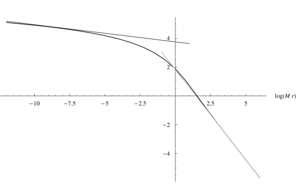
Figure 4: Flow $k=10$, logarithmic plot of the correlator $\langle\Psi(x)\Psi(0)\rangle$ (black line) together with both the IR (grey line) and the UV (dark-grey line) behaviours.

The inspection of the diagrams (see figures 1, 2, 3, 4, obtained for $k=1$, $2$, $3$, $10$ respectively) shows first of all the expected agreement in the IR limit: it is worth recalling that as in the case of the trace operator [1], the leading contribution of the spectral series is enough to obtain the exact IR power-law.

It is instead quite surprising that such an approximation is able to give a qualitative good agreement also in the UV (again similar to the case of the stress-energy tensor) when (14) is conjectured to give the correct power-law behaviour.

On the one hand, the previous result can be considered as a qualitative evidence that the operator $\sigma_{1}\Phi_{1,2}$ in the UV actually flows to the operator $\Phi_{2,1}$ in the IR theory. On the other hand, we would like to stress that such a result, being qualitative, is far from being neither conclusive nor satisfactory in the perspective of the identification of the UV operator $\sigma_{1}\Phi_{1,2}$. At best it can be viewed as an indication to stimulate the research of other, more reliable, methods to face the problem of the identification of operators in massless flows.

A final remark about the diagrams: since we are interested in the comparison of the slope of the curves, all the normalizations have been fixed in order to make such a comparison as clear as possible.

Concluding remarks

In this work, we constructed form factors of operators in the massless flow from the coset model $su(2)_{k+1}\otimes su(2)_{k}/su(2)_{2k+1}$ to the $M_{k+2}$ minimal model, mimicking the construction done in [4] of form factors of the magnetization operator and the energy operator in the massless flow
TIM $\to$ IM.

What we did in the section 1.2 is to look for solutions of the residue equation that are obtained replacing the $RR$ and $LL$ $S$-matrices $S^{RSOS}_{3}=-1$ by the $S^{RSOS}_{k+2}$-matrix, given that they should reproduce in the IR limit in both the right and left channel the form factors of the operator $\Phi_{1,2}$ in the minimal model $M_{k+2}$. Then we made a numerical check on the variation of conformal weight along the flow thanks to the $\Delta$-sum rule, and found that, if not excellent, it is compatible with the hypothesis that we are dealing with the operator $\Phi_{2,2}$ in the UV.

The situation is slightly more complicated in the section 2.2, because the asymptotic particles possesses generalized statistics for $k\neq 1$ : we took into account the IR properties only, and constructed form factors which in the IR limit reproduce the form factors of the parafermionic operators with conformal dimension $(\pm\Delta_{2,1},0)$ and $(0,\pm\Delta_{2,1})$. Notwithstanding this, the approximation of the two point function with the lowest form factor with one right and one left particle is enough to give, at least at a qualitative level, a good agreement with the power-law behaviour expected in the UV if we conjecture that the corresponding operator is $\sigma_{1}\Phi_{1,2}$.

We are not saying that we constructed all the possible flows of operators, but only those which have an obvious counterpart in the flow TIM $\to$ IM. It would be interesting to know what else could be constructed.

The results obtained in both [1] and the present work show that form factors in integrable massless models can provide important non perturbative information, even in more complicated cases than the flow TIM $\to$ IM. Obviously, we are in a privileged situation: having a one parameter family of flows at hand certainly allows us to understand better the loss of precision in the numerical tests for the $c$- and $\Delta$-sum rules as one increases the parameter $k$. Had we worked on the flow $\textrm{PCM}_{1}\to SU(2)_{1}$ only, the discrepancy of $43\%$ with respect to the exact value of the central charge [1] would have probably led us to conclude that our 4-particle form factor for the trace operator was wrong! Interestingly enough, the results of the present work as well as those of [19, 1] show that whether in the massive or the massless case, the truncation to the lowest form factor does not systematically give a ’very accurate’ approximation of the correlation function. One can really wonder up to what point it can be unaccurate; certainly, this means that one has to be rather cautious when interpreting the numerical results, in the case where a large discrepancy with respect to the expectations is observed.

We are aware of the fact that our task was considerably simplified as the flow is along $T\bar{T}$. For other integrable massless flows with a non diagonal $RL$ scattering, the situation is far more involved, both theoretically and numerically: in most cases, we do not expect that the lowest form factors can be nicely written as an explicit product of simple functions in the right and left channel as it is the case here; likely, even with the lowest number of particles one might not get rid of the integration variables, thus the integrals for the form factors should be evaluated numerically first.

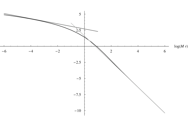
Figure 1: Flow $k=1$, logarithmic plot of the correlator $\langle\Psi(x)\Psi(0)\rangle$ (black line) together with both the IR (grey line) and the UV (dark-grey line) behaviours.

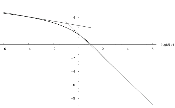
Figure 2: Flow $k=2$, logarithmic plot of the correlator $\langle\Psi(x)\Psi(0)\rangle$ (black line) together with both the IR (grey line) and the UV (dark-grey line) behaviours.

Figure 3: Flow $k=3$, logarithmic plot of the correlator $\langle\Psi(x)\Psi(0)\rangle$ (black line) together with both the IR (grey line) and the UV (dark-grey line) behaviours.

References

• [1] P. Grinza and B. Ponsot, ”Form factors in the massless coset models $su(2)_{k+1}\otimes su(2)_{k}/su(2)_{2k+1}$ - Part I”, [arXiv:hep-th/0411043], to appear in Nucl. Phys. B.
• [2] C. Crnkovic, G.M. Sotkov and M. Stanishkov, Phys. Lett. B226 (1989) 297.
• [3] P. Goddard, A. Kent and D.I. Olive, Phys.  Lett. B152 (1985) 88.
• [4] G. Delfino, G. Mussardo and P. Simonetti, Phys. Rev. D51 (1995) 6620 [arXiv:hep-th/9410117].
• [5] M. Karowski and P. Weisz, Nucl. Phys. B139 (1978) 455.
• [6] B. Berg, M. Karowski and P. Weisz, Phys. Rev. D19 (1979) 2477
• [7] F.A. Smirnov, ”Form factors in completely integrable models of Quantum Field theory”, Adv. Series in Math. Phys. 14, World Scientific 1992.
• [8] Al.B. Zamolodchikov, Nucl. Phys. B358 (1991) 524.
• [9] H. Babujian, A. Fring, M. Karowski and A. Zapletal, Nucl. Phys. B538 (1999) 535 [arXiv:hep-th/9805185].
• [10] H. Babujian and M. Karowski, Nucl. Phys. B620 (2002) 407 [arXiv:hep-th/0105178].
• [11] D. Bernard, Phys.  Lett.  B279 (1992) 78 [arXiv:hep-th/9201006].
• [12] A. LeClair, Phys.  Lett. B230 (1989) 103, D. Bernard and A. Leclair, Nucl. Phys. B340 (1990) 721, F.A. Smirnov, Int. J. Mod. Phys. A4 (1989) 4213 and Nucl. Phys. B337 (1990) 156
• [13] N.Yu. Reshetikhin and F.A. Smirnov, Commun. Math.  Phys. 131 (1990) 157.
• [14] A.B.  Zamolodchikov and Al.B.  Zamolodchikov, Nucl. Phys. B379 (1992) 602.
• [15] V.P. Yurov and Al.B. Zamolodchikov, Int. J. Mod. Phys. A6 (1991) 3419.
• [16] B. Ponsot, Phys. Lett. B575 (2003) 131 [arXiv:hep-th/0304240].
• [17] J.L. Cardy and G. Mussardo, Nucl. Phys. B340 (1990) 387.
• [18] S.L. Lukyanov, Mod. Phys. Lett. A12 (1997) 2543 [arXiv:hep-th/9703190].
• [19] B. Ponsot, “Form factors in the $SS$ model and its RSOS restrictions”, [arXiv:hep-th/0405218].
• [20] G. Delfino, P. Simonetti and J.L. Cardy, Phys. Lett. B387 (1996) 327 [arXiv:hep-th/9607046].
• [21] A.B. Zamolodchikov, Sov. J. Nucl. Phys. 46 (1987) 1090 [Yad. Fiz. 46 (1987) 1819].
• [22] A.W.W. Ludwig and J.L. Cardy, Nucl. Phys. B285 (1987) 687.
• [23] A.B. Zamolodchikov, Sov. J. Nucl. Phys. 44 (1986) 529 [Yad. Fiz. 44 (1986) 821].
• [24] T.R. Klassen and E. Melzer, Nucl. Phys. B370 (1992) 511.
• [25] R. Pogossyan, Sov. J. Nucl. Phys. 48 (1988) 763.
• [26] F.A. Smirnov, Commun. Math. Phys. 132 (1990) 415.
• [27] S.L. Lukyanov and A.B. Zamolodchikov, Nucl. Phys. B607 (2001) 437 [arXiv:hep-th/0102079].
Refer to caption