Semiclassical Bethe Ansatz and AdS/CFT

Abstract

The Bethe ansatz can be used to compute anomalous dimensions in ${\mathcal{N}}=4$ SYM theory. The classical solutions of the sigma-model on $AdS_{5}\times S^{5}$ can also be parameterized by an integral equation of Bethe type. In this note the relationship between the two Bethe ansätze is reviewed following hep-th/0402207.

1 Introduction

The string dual of the large-$N$ $\mathcal{N}=4$ super-Yang-Mills (SYM) theory has a geometric description in terms of the $AdS_{5}\times S^{5}$ background with RR flux [1, 2, 3]. The duality becomes especially simple at strong coupling or in the semiclassical limit [4, 5]. One of the surprising features of the semiclassical AdS/CFT correspondence is the appearance of integrable structures on both sides of the duality. The integrability arises as a quantum symmetry of operator mixing in CFT [6, 7, 8] and as a classical symmetry on the string world-sheet in AdS [9, 10]. This symmetry can be important in the quantum regime of AdS/CFT [11] and seemingly arises in other examples of the gauge/string theory duality [12].

The integrability implies that action-angle variables are globally defined and thus imposes strong restrictions on the classical dynamics. In many cases the separation of variables can be carried out even in quantum theory and then the spectrum can be found by purely algebraic means [13]. Typically, the spectrum is a Fock space of some elementary excitations whose creation-annihilation operators satisfy certain quadratic algebra. The algebra implies that momenta of elementary excitations in a physical state are subject to a set of algebraic constraints, the Bethe equations [14, 15]. The algebraic Bethe ansatz perhaps is the most generic way to quantize integrable systems. In the context of AdS/CFT, the Bethe ansatz proved instrumental in computing perturbative anomalous dimensions [16, 17, 18, 19, 20, 21, 22, 23, 24, 25, 26, 27, 28, 29] and OPE coefficients [30] of local operators in $\mathcal{N}=4$ SYM. The purpose of these notes, which are based on [21], is to explain how classical Bethe equations arise in string theory on $AdS_{5}\times S^{5}$. The quantum counterpart of these equations, if exists, should describe the exact spectrum of the AdS string or equivalently the non-perturbative spectrum of large-$N$ SYM. It is not clear how to derive such quantum Bethe ansatz, but the success of the discretized string Bethe equations [31] in reproducing the near-BMN spectrum of the string [32] can be taken as an indication that algebraic Bethe ansatz is indeed the right framework to deal with quantum string theory in $AdS_{5}\times S^{5}$.

2 Integrability in CFT

I will first explain how Bethe ansatz arises in perturbative SYM. It is especially useful in the semiclassical limit, which is accurate for states with large quantum numbers. There are two basic types of local operators with large quantum numbers in SYM. The majority of operators have large scaling dimensions at strong coupling [2], which is the stringy regime of AdS/CFT. This regime is non-perturbative by definition and hard to access by conventional field-theory methods. On the other hand, operators with a large number of constituent fields [4] can have huge global charges independently of the strength of interaction and are thus expected to behave stringy even in perturbation theory. The stringy behavior of both types of operators can be qualitatively explained by examining planar diagrams that dominate their correlation functions. Typical diagrams at strong coupling diagrams have large number of vertices and propagators and obviously resemble continuous string world-sheets. Planar diagrams for large operators always contain many of propagators and resemble continuous strings even at the lowest orders of perturbation theory.

The field content of $\mathcal{N}=4$ SYM theory consists of gauge fields $A_{\mu}$, six scalars $\Phi_{i}$ and four Majorana fermions $\Psi_{\alpha}^{A}$, all in the adjoint representation of $U(N)$. The action is

$$S=\frac{1}{g^{2}}\int d^{4}x\,\,{\rm tr}\,\left\{-\frac{1}{2}\,F_{\mu\nu}^{2}+(D_{\mu}\Phi_{i})^{2}+[\Phi_{i},\Phi_{j}]^{2}+{\rm fermions}\right\}.$$ (1)

The simplest local gauge-invariant operators are composed of two types of complex scalar fields $Z=\Phi_{1}+i\Phi_{2}$ and $W=\Phi_{3}+i\Phi_{4}$:

$$\mathcal{O}=\,{\rm tr}\,\left(Z^{L-M}W^{M}+{\rm permutations}\right).$$ (2)

These operators transform non-trivially under an $SU(2)\times U(1)$ subgroup of the $SO(6)$ R-symmetry. $(Z,W)$ transforms as a doublet of $SU(2)$ and has the $U(1)$ charge $1$. Correlation functions of operators (2) contain UV divergences and need to be regularized and renormalized by adding counterterms. In general the renormalized operator is a linear combination of several bare operators: $\mathcal{O}_{\boldsymbol{A}}=\boldsymbol{Z}_{\boldsymbol{A}}^{\hphantom{\boldsymbol{A}}\boldsymbol{B}}\mathcal{O}_{\boldsymbol{B}}^{\rm bare}$, where $\boldsymbol{A}$ and $\boldsymbol{B}$ are multi-indices that parameterize all possible operators with the same quantum numbers (the same number of $Z$ and $W$ fields in the present case). The mixing matrix is defined as $\Gamma=\boldsymbol{Z}^{-1}d\boldsymbol{Z}/d\ln\Lambda$, where $\Lambda$ is a UV cutoff. Its eigenvectors are conformal operators and its eigenvalues are their anomalous dimensions: $\Gamma_{\boldsymbol{A}}^{\hphantom{\boldsymbol{A}}\boldsymbol{B}}\mathcal{O}^{(n)}_{\boldsymbol{B}}=\gamma_{n}\mathcal{O}^{(n)}_{\boldsymbol{A}}$, so that the scaling dimension of the operator $\mathcal{O}^{(n)}$ is $\Delta_{n}=L+\gamma_{n}$. The set of operators (2) is closed under renormalization. Operators from this set do not mix with operators that contain $F_{\mu\nu}$, fermions or derivatives [33, 34]. Including such operators is possible [33, 8, 35, 34] but will not be discussed here for the sake of simplicity.

The number of operators of the same length $L$ grows very quickly with $L$, which makes perturbation theory for large operators highly degenerate. Thus computation of anomalous dimensions is a non-trivial problem for large operators even at one loop. The following parametrization of operators (2) enormously simplifies this problem. Let us associate the field $Z$ with spin up and the field $W$ with spin down. An operator of the form (2) then defines a distribution of spins on a periodic one-dimensional lattice of length $L$:

$$\,{\rm tr}\,ZZZWWZZZWWWZWZZZZ\ldots\qquad\longleftrightarrow\qquad\left|\uparrow\uparrow\uparrow\downarrow\downarrow\uparrow\uparrow\uparrow\downarrow\downarrow\downarrow\uparrow\downarrow\uparrow\uparrow\uparrow\uparrow\ldots\right\rangle.$$

The map between the operators and the states of the spin chain is one-to-one if the states are required to be translationally invariant. The mixing matrix acts linearly on the operators and thus can be interpreted as a Hamiltonian of a spin chain.

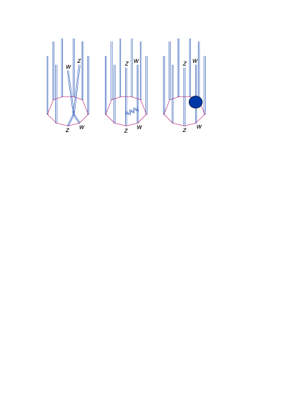
Figure 1: The one-loop diagrams.

The one-loop mixing matrix can be easily computed. The three diagrams that contribute at this order are shown in fig. 1. The gluon exchange and the self-energy produce the same renormalized operator, while the scalar vertex can lead to the interchange of $Z$ and $W$ fields. At large $N$ the interchange can only occur between adjacent sites of the lattice. Indeed, an insertion of the vertex between a pair propagators produces a non-planar graph unless the propagators start from the adjacent sites. The planar mixing matrix is thus a Hamiltonian of a spin chain with nearest-neighbor interactions. Explicitly [6],

$$\Gamma=\frac{\lambda}{8\pi^{2}}\sum_{l=1}^{L}(1-P_{l,l+1}),$$ (3)

where $\lambda=g^{2}N$ is the ’t Hooft coupling and $P$ is the permutation operator: $P\,a\otimes b=b\otimes a$. The use of the identity $P=(1+\boldsymbol{\sigma}\otimes\boldsymbol{\sigma})/2$ brings the mixing matrix to the familiar form of the Heisenberg Hamiltonian:

$$\Gamma=\frac{\lambda}{16\pi^{2}}\sum_{l=1}^{L}(1-\boldsymbol{\sigma}_{l}\cdot\boldsymbol{\sigma}_{l+1}).$$ (4)

The physical states that describe operators in the SYM theory should satisfy an additional constraint:

$$U\left|{\rm phys}\right\rangle=\left|{\rm phys}\right\rangle,$$ (5)

where $U$ is the shift operator: $U^{-1}\boldsymbol{\sigma}_{l}U=\boldsymbol{\sigma}_{l-1}$. The eigenvalues of $U$ define the total momentum which must be zero (or an integer multiple of $2\pi$) for translationally invariant physical states.

Though Heisenberg Hamiltonian contains no adjustable parameters except for the length of the chain it is possible to identify several energy scales in its spectrum (fig. 2). The ground state is the ferromagnetic vacuum (all spins up) and corresponds to a chiral primary operator $\,{\rm tr}\,Z^{L}$. This operator belongs to a short multiplet of $\mathcal{N}=4$ supersymmetry and has zero anomalous dimension to all orders in perturbation theory. In particular it has zero anomalous dimension at one loop, so the ground state of the spin chain has zero energy. The excited states are obtained by flipping one or more spins. In some approximation the spectrum is generated by

$$a^{\dagger}_{n}=\frac{1}{\sqrt{L}}\sum_{l=1}^{L}\e^{\frac{2\pi inl}{L}}\sigma^{-}_{l}.$$ (6)

The operator $a^{\dagger}_{n}$ creates a magnon with the mode number $n$ and the momentum $p=2\pi n/L$. If $L$ is sufficiently large, Fock states $a^{\dagger}_{n_{1}}\ldots a^{\dagger}_{n_{M}}\left|0\right\rangle$ (with $M\ll L$) approximate the eigenstates of the Heisenberg Hamiltonian up to computable $1/L$ corrections [27]. The multi-magnon states correspond to the BMN operators [4] and are dual to string states in the pp-wave limit of the $AdS_{5}\times S^{5}$ geometry [36]. The anomalous dimensions of the BMN operators (the energies of magnons),

$$\gamma=\frac{\lambda}{2L^{2}}\sum_{k=1}^{M}n_{k}^{2},$$ (7)

match with the energies of the string oscillators [4]. The zero-momentum condition becomes the level matching condition on the string side.

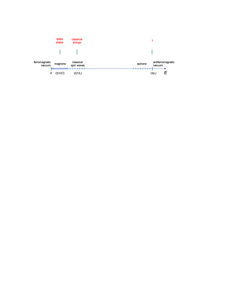
Figure 2: The spectrum of the Heisenberg spin chain.

The situation changes when the number of magnons becomes macroscopically large: $M\sim L$. Then the interaction between magnons cannot be neglected any more and the Fock space generated by simple operators (6) is no longer a good approximation for the spectrum. The remarkable property of the Heisenberg model, which stems from its completely integrability, is that the exact spectrum is still a Fock space. The simple creation operators (6) get dressed by interactions, but the exact spectrum-generating operators still obey relatively simple exchange relations (the Yang-Baxter algebra) and the spectrum can be computed algebraically. The energy eigenstates as before are parameterized by momenta of individual magnons, but now the momenta satisfy a set of algebraic equations [14, 15]:

$$\left(u_{j}+i/2\over u_{j}-i/2\right)^{L}=\prod_{k\neq j}{u_{j}-u_{k}+i\over u_{j}-u_{k}-i}.$$ (8)

The Bethe roots $u_{j}$, $j=1,\ldots,M$ are distinct complex numbers which parameterize the momenta of magnons:

$$\e^{ip}={u+i/2\over u-i/2}.$$

The momentum constraint takes the form

$$\prod_{j}{u_{j}+i/2\over u_{j}-i/2}=1,$$ (9)

and the anomalous dimension is computed as

$$\gamma={\lambda\over 8\pi^{2}}\sum_{j}{1\over u_{j}^{2}+1/4}\,.$$ (10)

The simplest solution of the Bethe equations that satisfies the momentum constraint contains two roots, which describes two magnons with opposite momenta:

$$u_{1}=-u_{2}=\frac{1}{2}\,\cot\frac{\pi n}{L-1},\qquad n=1,2,\ldots$$ (11)

The anomalous dimension is

$$\gamma=\frac{\lambda}{\pi^{2}}\,\sin^{2}\frac{\pi n}{L-1}\,.$$ (12)

When $L$ is large, $u_{1,2}\approx\pm L/2\pi n$ and we get back to the BMN formula (7). The fact that Bethe roots scale as $u_{i}\sim L$ is true for all BMN-like states. The right hand side of Bethe equations can then be replaced by $1$, or in other words the interaction between magnons can be neglected. A little complication occurs when more than one magnon occupies the same momentum state. Then the above argument does not apply since magnons cannot have the same rapidities. As a result, the rapidities split in the complex plane and magnons with the same momentum form a bound state. Because $(u+i/2)/(u-i/2)$ is no longer a pure phase, the left hand side of (8) turns to zero or to infinity as $L\rightarrow\infty$. This should be compensated by a zero or a pole on the right hand side, which can only happen if two or more rapidities are separated by $\pm i$. The rapidities of magnons in the bound state thus form a rigid array with two or more roots at $u_{\rm c.m.}+ir$, where $r$ are integers or half-integers. Such arrays are usually called strings. The number of roots in a string can be arbitrary, even macroscopically large [37] (fig. 3). In the latter case strings bend on the macroscopic scales and form some contours in the complex plane. The corresponding Bethe states describe macroscopic spin waves and are dual to semiclassical strings in $AdS_{5}\times S^{5}$ [38, 16].

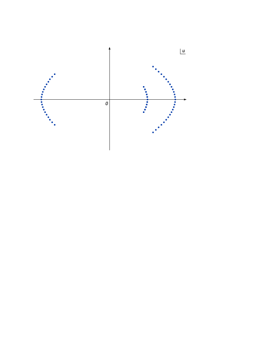
Figure 3: Macroscopically large Bethe strings.

Since Bethe roots scale linearly with $L$, it is natural to define $x_{i}=u_{i}/L$, which stays finite at $L\rightarrow\infty$. Taking the logarithm of (8) and expanding in $1/L$, we get

$${1\over x_{j}}+2\pi n_{j}={1\over L}\sum_{k\neq j}{2\over x_{j}-x_{k}},$$ (13)

where the phases $2\pi n_{j}$ parameterize the branches of the logarithm. The mode numbers $n_{j}$ are different for different Bethe strings. The distance between the adjacent roots scales as $x_{k}-x_{k+1}\sim 1/L$, so the distribution of roots can be characterized by a continuous density in the scaling limit:

$$\rho(x)=\frac{1}{L}\sum_{j}\delta(x-x_{j}).$$ (14)

The density is defined on a collection of contours $C=C_{1}\cup\ldots\cup C_{K}$ in the complex plane and is normalized as

$$\int_{C}dx\rho(x)=\frac{M}{L}\,,$$ (15)

where $M$ is the total number of magnons, or the number of $W$ fields in the operator (2). Equivalently, the distribution of Bethe roots can be characterized by the resolvent:

$$G(x)=\frac{1}{L}\sum_{j}\frac{1}{x-x_{j}}=\int_{C}dy\,\frac{\rho(y)}{x-y}\,.$$ (16)

The Taylor expansion of $G(x)$ at zero generates local conserved charges of the Heisenberg model [39, 18]. In particular, the total momentum is $-G(0)$. Translational invariance then requires

$$-G(0)=\int_{C}dx\,\frac{\rho(x)}{x}=2\pi m.$$ (17)

The next Taylor coefficient determines the anomalous dimension:

$$\Delta-L=\frac{\lambda}{8\pi^{2}L}\int_{C}dx\,\frac{\rho(x)}{x^{2}}\,.$$ (18)

The Bethe equations reduce to a singular integral equation for the density:

$${-\!\!\!\!\!\!\int}_{{\bf C}}{dy\,\rho(y)\over x-y}={1\over x}+2\pi n_{k},\qquad x\in C_{k},$$ (19)

which resembles the saddle-point equation for a distribution of eigenvalues of a random matrix [40]. Its general solution is known and can be expressed in terms of the hyperelliptic integrals [21]. The associated Riemann surface is obtained by gluing together two copies of the complex plane with cuts along the contours $C_{k}$.

The one- and two-cut solutions (rational and elliptic cases) were worked out in [16, 17, 21] and were compared to the Frolov-Tseytlin string solutions [38]. $1/L$ corrections, that can be explicitly calculated in the simplest rational case [23], on the string side correspond to quantum corrections on the world sheet [41]. The scaling dimensions of operators were found to agree with the energies of the string states up to two loops. At three loops the agreement breaks down for the BMN states [32] and for the macroscopic strings [19, 22, 42], but the two-loop agreement can be established quite generally at the level of the effective actions [43] or the equations of motion [44]. Even the higher charges of the integrable hierarchies, that do not have geometric interpretation in AdS/CFT, were found to agree [39, 45]. The classical solutions of the sigma-model can also be parameterized by an integral equation of Bethe type. Such an equation was derived for strings on $S^{3}\times\mathbb{R}^{1}$ [21], $AdS_{3}\times S^{1}$ [28] and $S^{5}\times\mathbb{R}^{1}$ [29]. I will discuss the first case.

3 Integrability in AdS

The R-charges of the operator $\,{\rm tr}\,(Z^{L-M}W^{M}+\ldots)$, $L$ and $M$, are dual to angular momenta of the string on $S^{5}$. The string in the middle of $AdS_{5}$ has two non-zero angular momenta if it moves in $S^{3}\subset S^{5}$. The world sheet is then parameterized by the global AdS time $X^{0}$ and by four Cartesian coordinates $X^{i}$ constrained by $X^{i}X^{i}=1$. A point on the three-sphere defines a group element of $SU(2)$:

$$g=\left(\begin{array}[]{cc}X_{1}+iX_{2}&X_{3}+iX_{4}\\ -X_{3}+iX_{4}&X_{1}-iX_{2}\end{array}\right)\equiv\left(\begin{array}[]{cc}Z_{1}&Z_{2}\\ -{\bar{Z}}_{2}&{\bar{Z}}_{1}\end{array}\right)\in SU(2),$$ (20)

and the equations of motion of the string can be conveniently formulated in terms of the currents

$$j_{a}=g^{-1}\partial_{a}g={\sigma^{A}\over 2i}\,j^{A}_{a}.$$ (21)

The relevant part of the string action takes the following form in the conformal gauge:

$$S_{\sigma m}=-\frac{\sqrt{\lambda}}{4\pi}\int_{0}^{2\pi}d\sigma\int d\tau\,\left[\frac{1}{2}\,{\rm Tr}j_{a}^{2}+(\partial_{a}X_{0})^{2}\right].$$ (22)

The equations of motion are

$$\partial_{+}\partial_{-}X_{0}=0,$$ (23)

$$\partial_{+}j_{-}+\partial_{-}j_{+}=0,$$ (24)

where $\partial_{\pm}=\partial_{\tau}\pm\partial_{\sigma}$ and $j_{\pm}=j_{\tau}\pm j_{\sigma}$. The currents are flat as a consequence of their definition:

$$\partial_{+}j_{-}-\partial_{-}j_{+}+[j_{+},j_{-}]=0,$$ (25)

The equations of motion should be supplemented by Virasoro constraints

$$\frac{1}{2}\,\,{\rm tr}\,j_{\pm}^{2}=-(\partial_{\pm}X^{0})^{2}.$$ (26)

Since (23) is trivially solved by

$$X^{0}=\kappa\tau,$$

we find:

$$\frac{1}{2}\,\,{\rm tr}\,j_{\pm}^{2}=-\kappa^{2}.$$ (27)

The global symmetry of the sigma-model (22) is $SU_{L}(2)\times SU_{R}(2)\times\mathbb{R}$. The first two factors are associated with the left and right group multiplications: $g\rightarrow hg$ and $g\rightarrow gh$. The Noether currents of these symmetries are $l_{a}$ and $j_{a}$, where $j_{a}$ is defined in (21) and

$$l_{a}=gj_{a}g^{-1}=\partial_{a}g\,g^{-1}={\sigma^{A}\over 2i}\,l^{A}_{a}.$$ (28)

Therefore the Noether charges

$$Q_{L}^{A}=\frac{\sqrt{\lambda}}{4\pi}\int_{0}^{2\pi}d\sigma\,l^{A}_{\tau},\qquad Q_{R}^{A}=\frac{\sqrt{\lambda}}{4\pi}\int_{0}^{2\pi}d\sigma\,j^{A}_{\tau}$$ (29)

generate the left and right group shifts. The dual R-charges in the SYM theory can be easily identified. The scalars of the SYM and the Cartesian coordinates on the sphere transform in the same way under $SO(6)$: $\Phi_{i}\sim X^{i}$. Since $Z=\Phi_{1}+i\Phi_{2}$ and $W=\Phi_{3}+i\Phi_{4}$, these fields transform as $Z_{1}$ and $Z_{2}$ in (20). Thus $(Z_{1},Z_{2})$ and $(Z,W)$ are doublets of $SU_{R}(2)$, so that $Z$ has $Q^{3}_{R}=1$ and $W$ and $Q^{3}_{R}=-1$. For the string dual of the operator (2) we thus have

$$Q^{3}_{R}=L-2M.$$ (30)

Under the left shifts $(Z_{1},-\bar{Z}_{2})$ and $(Z_{2},-\bar{Z}_{1})$ transform as doublets. Therefore, $(Z,-\bar{W})$ and $(W,-\bar{Z})$ are doublets of $SU_{L}(2)$ and both fields $Z$ and $W$ have $Q^{3}_{L}=1$. Hence the left charge of the operator (2) is just the length of the spin chain:

$$Q^{3}_{L}=L.$$ (31)

The time translations $X^{0}\rightarrow X^{0}+t$ generate scale transformations on the boundary of $AdS_{5}$, and the energy of the string should be identified with the scaling dimension of the dual operator:

$$\Delta=\frac{\sqrt{\lambda}}{2\pi}\int_{0}^{2\pi}d\sigma\,\partial_{\tau}X_{0}=\sqrt{\lambda}\,\kappa.$$ (32)

The equations of motion for the chiral field (24), (25) are completely integrable [46] and can be effectively linearized with the help of the inverse scattering transformation [47]. The method is based on the zero-curvature representation [48] introduced for the sigma-model in [49]. The rescaled currents [49]

$$J_{\pm}(x)=\frac{j_{\pm}}{1\mp x}$$ (33)

are flat for any value of $x$:

$$\partial_{+}J_{-}-\partial_{-}J_{+}+[J_{+},J_{-}]=0,$$ (34)

as a consequence of the equations of motion. On the other hand, if (34) is satisfied for any $x$, then $j_{\pm}$ are solutions of the equations of motion. The equations of motion (24) and (25) and the flatness condition (34) are thus completely equivalent.

The monodromy of the flat connection (33) defines the quasi-momentum $p(x)$:

$$\Omega(x)=P\exp\left(-\int_{0}^{2\pi}d\sigma\,J_{\sigma}\right)=P\exp\int_{0}^{2\pi}d\sigma\,\frac{1}{2}\left({j_{+}\over x-1}+{j_{-}\over x+1}\right),$$ (35)

$$\,{\rm tr}\,\Omega(x)=2\cos p(x),$$ (36)

where the integral is taken along a fixed-time section of the world-sheet. The quasi-momentum is a functional of the world-sheet currents and potentially depends on time. The key point is that it becomes time-independent on-shell. Indeed, the trace of the holonomy of a flat connection does not depend on the contour of integration. Shifting the time slice along which the flat connection is integrated changes nothing and therefore the quasi-momentum is conserved as soon as the equations of motion are satisfied. It can thus be regarded as a generating function for an infinite set of integrals of motion.

The $SU_{L,R}(2)$ charges appear in the expansion of $p(x)$ at zero and at infinity. At infinity: $J_{\sigma}(x)=j_{\tau}/x+\ldots$, so

$$\,{\rm tr}\,\Omega=2+\frac{1}{2x^{2}}\int_{0}^{2\pi}d\sigma_{1}d\sigma_{2}\,\,{\rm tr}\,j_{\tau}(\sigma_{1})j_{\tau}(\sigma_{2})+\ldots=2-\frac{4\pi^{2}Q_{R}^{2}}{\lambda x^{2}}+\ldots=2-\frac{4\pi^{2}(L-2M)^{2}}{\lambda x^{2}}+\ldots\,.$$ (37)

Hence,

$$p(x)=-\frac{2\pi(L-2M)}{\sqrt{\lambda}\,x}+\ldots\qquad(x\rightarrow\infty).$$ (38)

Further terms in the expansion of the monodromy matrix $\Omega(x)$ generate Yangian charges, which potentially play an important role in the AdS/CFT correspondence [11, 50].

At $x\rightarrow 0$, $\partial_{\sigma}+J_{\sigma}(x)=\partial_{\sigma}+j_{\sigma}-xj_{\tau}+\ldots=g^{-1}(\partial_{\sigma}-xl_{\tau}+\ldots)g$, so

$$\,{\rm tr}\,\Omega=2+\frac{x^{2}}{2}\int_{0}^{2\pi}d\sigma_{1}d\sigma_{2}\,\,{\rm tr}\,l_{\tau}(\sigma_{1})l_{\tau}(\sigma_{2})+\ldots=2-\frac{4\pi^{2}Q_{L}^{2}}{\lambda}\,x^{2}+\ldots=2-\frac{4\pi^{2}L^{2}}{\lambda}\,x^{2}+\ldots\,,$$ (39)

which yields

$$p(x)=2\pi m+\frac{2\pi L}{\sqrt{\lambda}}\,x+\ldots\qquad(x\rightarrow 0),$$ (40)

where $m$ is an arbitrary integer.

The local charges can be obtained by expanding the quasi-momentum in the Lorant series at $x=\pm 1$ for a systematic recursive procedure exists [48]. A slightly different but equivalent definition of the quasi-momentum is more appropriate for that purpose. Let us consider the auxiliary linear problem

$$\left[\partial_{\sigma}-\frac{1}{2}\left({j_{+}\over x-1}+{j_{-}\over x+1}\right)\right]\psi=0,$$ (41)

where $\psi(\sigma;x)$ is a two-component vector ($j_{\pm}$ are anti-Hermitian $2\times 2$ matrices). This equation can be regarded as a spectral problem for a one-dimensional Dirac operator with a periodic potential, where $x$ plays the role of the spectral parameter. Two linearly independent solutions of this spectral problem can be chosen quasi-periodic: $\psi(\sigma+2\pi;x)=\e^{\pm ip(x)}\psi(\sigma;x)$. This is the standard definition of the quasi-momentum. It is easy to see that the previous definition is equivalent to that. Indeed, $\psi(\sigma+2\pi;x)=\Omega(x)\psi(\sigma;x)$ in any basis, even in which the wave function is not quasi-periodic. Requirement of quasi-periodicity is equivalent to diagonalization of the monodromy matrix whose eigenvalues are precisely $\e^{\pm ip(x)}$.

When $x$ is close to $+1$ or $-1$, the linear problem (41) can be solved in the WKB approximation, because it takes the form

$$\left(i\hbar\partial_{\sigma}+V\right)\psi=0,$$ (42)

where $\hbar\equiv 4(x\pm 1)\rightarrow 0$ and

$$V=u^{A}\sigma^{A},\qquad u^{A}=-j^{A}_{\mp}\pm\frac{\hbar}{8\mp\hbar}\,j^{A}_{\pm}.$$ (43)

Plugging the WKB ansatz $\psi=\e^{iS/\hbar}\chi$ into (42), we find that

$$\left(V-\partial_{\sigma}S\right)\chi=0.$$ (44)

Thus $\chi$ is an eigenvector of $V$ with the eigenvalue $\partial_{\sigma}S$. Using the Virasoro constraints (26) we find that the two eigenvalues of $V$ are $\pm 2\kappa+O(\hbar)$. Choosing the upper sign we get $S(\sigma)=\kappa\sigma$, $\psi=\,{\rm e}\,^{i\kappa\sigma/2(x\pm 1)}$ and

$$\psi(\sigma+2\pi;x)=\exp\left(\frac{i\pi\kappa}{x\pm 1}\right)\psi(\sigma;x).$$

Therefore

$$p(x)=-\frac{\pi\kappa}{x\pm 1}+\ldots\qquad(x\rightarrow\mp 1).$$ (45)

Let me make a short digression on the higher orders of the WKB expansion. The first non-trivial charges arise at $O(\hbar^{0})$ and can be interpreted as the energy and momentum [54]. Those are not the standard Noether charges one would get from the sigma-model action (22) and they generate the equations of motion (24), (25) only if the Poisson structure is properly modified [54]. Since these facts may have important implications for quantization, I will rederive them from the observation that the $O(\hbar^{0})$ correction to the quasi-momentum is the Berry’s phase. The $O(\hbar)$ charges are explicitly calculated in [29] for a more general case of the $SO(6)$ sigma-model.

The monodromy matrix, defined as

$$T(\sigma;x)=P\exp\int_{0}^{\sigma}d\tilde{\sigma}\,\frac{1}{2}\left({j_{+}\over x-1}+{j_{-}\over x+1}\right),$$ (46)

is a solution of (41) with the initial condition $T(0;x)={\mathbb{1}}$. This object is a generalization of (35): $\Omega(x)=T(2\pi;x)$. In the semiclassical approximation,

$$T(\sigma)=\sum_{n}\exp\left({\frac{i}{\hbar}\,\int_{0}^{\sigma}d\tilde{\sigma}\,\mu_{n}(\tilde{\sigma})}\right)\chi_{n}(\sigma)\chi_{n}^{\dagger}(0),$$ (47)

where $\chi_{n}(\sigma)$ and $\mu_{n}(\sigma)$ are the normalized eigenvectors and eigenvalues of $V(\sigma)$:

$$V\chi_{n}=\mu_{n}\chi_{n},$$

which depend on $\sigma$ as a parameter. The representation (47) follows from (44) and is accurate up to $O(\hbar)$ corrections.

Though matrix elements of $V$ are periodic functions of $\sigma$, the eigenvectors of $V$ are only quasi-periodic. It is well known that the transport of an eigenvector $\chi_{n}$ around a closed contour in the parameter space generates a geometric Berry’s phase [55]:

$$\chi_{n}(\sigma+2\pi)=\e^{i\gamma_{n}}\chi_{n}(\sigma),$$ (48)

which cannot be written as a local functional of the matrix elements of $V(\sigma)$. The best one can do is analytically continue $V(\sigma)$ into the interior of the unit disc whose boundary is the circle parameterized by $\sigma$. Then [55]

$$\gamma_{n}=2{\mathop{\mathrm{Im}}\nolimits}\int_{0}^{2\pi}d\sigma\,\int_{0}^{1}d\xi\,\sum_{m\neq n}\frac{\left\langle n\right|\frac{\partial V}{\partial\xi}\left|m\right\rangle\,\left\langle m\right|\frac{\partial V}{\partial\sigma}\left|n\right\rangle}{(\mu_{n}-\mu_{m})^{2}}\,,$$ (49)

where $\xi$ is the radial variable. The phase mod $2\pi$ does not depend on how $V$ is continued into the interior of the disc as long as the continuation is analytic.

Because $V$ is traceless, its two eigenvalues are equal in magnitude and opposite in sign: $\mu_{1}=-\mu_{2}\equiv\mu$. The same is true for the Berry’s phases: $\gamma_{1}=-\gamma_{2}\equiv\gamma$. From (36), (47) and (48) we find that

$$p(x)=-\frac{1}{4(x\pm 1)}\int_{0}^{2\pi}d\sigma\,\mu(\sigma;x)-\gamma(x)+O\left(x\pm 1\right).$$ (50)

There are two sources of $O(1)$ terms in the quasimomentum: the Berry’s phase and the subleading term in the expansion of the eigenvalue $\mu=u\equiv\sqrt{u^{A}u^{A}}$:

$$\mu=2\kappa\mp\frac{\hbar}{16\kappa}\,j_{+}^{A}j_{-}^{A}+O(\hbar^{2}).$$ (51)

The Berry’s phase can be calculated from (49):

$$\gamma=\frac{1}{2}\int_{0}^{2\pi}d\sigma\,\int_{0}^{1}d\xi\,\varepsilon^{ABC}\,\frac{u^{A}}{u^{3}}\,\frac{\partial u^{B}}{\partial\xi}\frac{\partial u^{C}}{\partial\sigma}=-\frac{1}{16\kappa^{3}}\int_{0}^{2\pi}d\sigma\,\int_{0}^{1}d\xi\,\varepsilon^{ABC}j_{\mp}^{A}\,\frac{\partial j_{\mp}^{B}}{\partial\xi}\frac{\partial j_{\mp}^{C}}{\partial\sigma}+O(\hbar)$$ (52)

This gives two conserved charges:

$$P_{\pm}=\int_{0}^{2\pi}d\sigma\left(\frac{1}{4\kappa^{2}}\int_{0}^{1}d\xi\,\varepsilon^{ABC}j_{\pm}^{A}\,\frac{\partial j_{\pm}^{B}}{\partial\xi}\frac{\partial j_{\pm}^{C}}{\partial\sigma}\pm\frac{1}{4}\,j_{+}^{A}j_{-}^{A}\right).$$ (53)

Their linear combinations can be interpreted as the energy and momentum [54]:

$$H = \int_{0}^{2\pi}d\sigma\left[\frac{1}{4\kappa^{2}}\int_{0}^{1}d\xi\,\varepsilon^{ABC}\left(j_{+}^{A}\,\frac{\partial j_{+}^{B}}{\partial\xi}\frac{\partial j_{+}^{C}}{\partial\sigma}-j_{-}^{A}\,\frac{\partial j_{-}^{B}}{\partial\xi}\frac{\partial j_{-}^{C}}{\partial\sigma}\right)+\frac{1}{2}\,j_{+}^{A}j_{-}^{A}\right],$$ (54)

$$P = \frac{1}{4\kappa^{2}}\int_{0}^{2\pi}d\sigma\int_{0}^{1}d\xi\,\varepsilon^{ABC}\left(j_{+}^{A}\,\frac{\partial j_{+}^{B}}{\partial\xi}\frac{\partial j_{+}^{C}}{\partial\sigma}+j_{-}^{A}\,\frac{\partial j_{-}^{B}}{\partial\xi}\frac{\partial j_{-}^{C}}{\partial\sigma}\right).$$ (55)

These are not the standard momentum and energy of the sigma-model (22). The latter are trivial as long as the Virasoro constraints are imposed. $P$ generates translations and $H$ generates the equations of motion (24), (25), if the Poisson brackets of the currents are defined to be

$$\{j_{\pm}^{A}(\sigma),j_{\pm}^{B}(\sigma^{\prime})\}=\varepsilon^{ABC}\delta(\sigma-\sigma^{\prime})j_{\pm}^{C}(\sigma),\qquad\{j_{+}^{A}(\sigma),j_{-}^{B}(\sigma^{\prime})\}=0.$$ (56)

One would get different Poisson brackets, which contain $\delta^{\prime}(\sigma-\sigma^{\prime})$, from the action (22). It was argued in [54] that the non-standard Poisson structure (56) is more consistent with integrability than the standard Poisson structure and is better suited for quantization when the constraints (26) are imposed.

Let us now return to the linear problem (41). Its spectrum has a band structure, but since the Dirac operator in (41) does not possess any particular Hermiticity properties, the allowed bands do not lie on the real axis. Instead, they form symmetric contours in the complex plane. The quasi-momentum is real: $\,{\rm tr}\,\Omega\in\mathbb{R}$ and $|\,{\rm tr}\,\Omega|<2$ on the allowed zones. Forbidden zones can be defined as contours on which the quasi-momentum is pure imaginary: $\,{\rm tr}\,\Omega\in\mathbb{R}$, $|\,{\rm tr}\,\Omega|>2$. At zone boundaries $\,{\rm tr}\,\Omega=2$ and the monodromy matrix $\Omega$ degenerates into a Jordan cell. The two quasi-periodic solutions of the Dirac equation, let us denote them $\psi_{\pm}(\sigma;x)$, become degenerate there. Encircling a zone boundary in the complex plane of $x$ interchanges the two solutions, so zone boundaries are branch points of $\psi_{\pm}(x)$. By cutting two copies of the complex plane along the forbidden zones and gluing them together we get a Riemann surface on which $\psi_{\pm}$ are globally defined as two branches of a single meromorphic function. The same is true for the eigenvalues of the monodromy matrix $\e^{\pm ip(x)}$. The trace of the monodromy matrix $\,{\rm tr}\,\Omega(x)$ has an essential singularity at $x=\pm 1$, where the Dirac operator has a pole, but otherwise $\,{\rm tr}\,\Omega(x)$ is a holomorphic function of $x$. The branch points arise when we solve $\e^{ip}+\e^{-ip}=\,{\rm tr}\,\Omega$ for $\e^{ip}$ precisely at the zone boundaries where $\,{\rm tr}\,\Omega=2$.

A particular branch of the quasi-momentum $p(x)$ is an analytic function of $x$ on the complex plane with cuts and has single poles at $x=\pm 1$. Subtracting the poles we get a function

$$G(x)=p(x)+\frac{\pi\kappa}{x-1}+\frac{\pi\kappa}{x+1},$$ (57)

which has only branch cut singularities and therefore is completely determined by its discontinuities: $G(x+i0)-G(x-i0)\equiv 2i\pi\rho(x)$. It is straightforward to prove that $G(x)$ admits the dispersion representation

$$G(x)=\int_{C}dy\,\frac{\rho(y)}{x-y}\,.$$ (58)

As a consequence of the spectral representation (58), the density $\rho(x)$ satisfies an integral equation which reflects the unimodularity of the monodromy matrix. To derive this equation, let us consider the behavior of the quasi-momentum near a forbidden zone where the quasi-momentum experiences a jump. The two branches of the double-valued analytic function $\e^{ip(x\pm i0)}$ are the two eigenvalues of the monodromy matrix $\Omega(x)$ and thus satisfy $\e^{ip(x+i0)}\e^{ip(x-i0)}=1$, or

$$p(x+i0)+p(x-i0)=2\pi n_{k},\qquad x\in C_{k},$$ (59)

on all of the forbidden zones. Taking into account (57) and (58), we get

$$2{-\!\!\!\!\!\!\int}dy\,\frac{\rho(y)}{x-y}=\frac{2\pi\kappa}{x-1}+\frac{2\pi\kappa}{x+1}+2\pi n_{k},\qquad x\in C_{k}.$$ (60)

The density also satisfies several normalization conditions which follow from (38), (40) and (45):

$$\int dx\,\rho(x) = \frac{2\pi}{\sqrt{\lambda}}(\Delta+2M-L),$$ (61)

$$\int dx\,\frac{\rho(x)}{x} = 2\pi m,$$ (62)

$$\int dx\,\frac{\rho(x)}{x^{2}} = \frac{2\pi}{\sqrt{\lambda}}(\Delta-L).$$ (63)

The equations (60)–(63) are very similar to the classical Bethe equations for the spin chain. The change of variables $x\rightarrow 4\pi Lx/\sqrt{\lambda}$ explicitly relates the two sets of equations:

$$2{-\!\!\!\!\!\!\int}dy\,\frac{\rho(y)}{x-y} = \frac{x}{x^{2}-\frac{\lambda}{16\pi^{2}L^{2}}}\,\,\frac{\Delta}{L}+2\pi n_{k},\qquad x\in C_{k},$$ (64)

$$\int dx\,\rho(x) = \frac{M}{L}+\frac{\Delta-L}{2L}\,,$$ (65)

$$\int dx\,\frac{\rho(x)}{x} = 2\pi m,$$ (66)

$$\Delta-L = \frac{\lambda}{8\pi^{2}L}\int dx\,\frac{\rho(x)}{x^{2}}\,.$$ (67)

The one-loop classical Bethe ansatz (19), (15), (17) and (18) is recovered in the limit $\lambda/L^{2}\rightarrow 0$.

4 Discussion

The main result of the long derivation in sec. 3 is an integral equation that parameterizes classical solutions of the sigma-model [21]:

$$2{-\!\!\!\!\!\!\int}dy\,\frac{\rho(y)}{x-y}=\frac{x}{x^{2}-\frac{\lambda}{16\pi^{2}L^{2}}}\,\,\frac{\Delta}{L}+2\pi n_{k}.$$ (68)

This equation reduces at $\lambda/L^{2}\rightarrow 0$ to the classical Bethe equation for the spin chain:

$$2{-\!\!\!\!\!\!\int}dy\,\frac{\rho(y)}{x-y}=\frac{1}{x}+2\pi n_{k}.$$ (69)

That equation in turn is an approximation to the exact quantum Bethe equations

$$\left(u_{j}+i/2\over u_{j}-i/2\right)^{L}=\prod_{k\neq j}{u_{j}-u_{k}+i\over u_{j}-u_{k}-i}\,.$$ (70)

In view of the analogy between (68) and (69), it is natural to ask if (68) is a scaling limit of some discrete Bethe equations which describe the full quantum spectrum of the AdS string. Potentially useful analogy in this respect is the $SU(2)$ chiral field (sigma-model on $S^{3}$) which classically is a subsector of the full $AdS_{5}\times S^{5}$ sigma-model. The quantum chiral field can be fermionized and solved by Bethe ansatz [56]. Perhaps the sigma-model in $AdS_{5}\times S^{5}$ can also be fermi/bosonized and solved by similar techniques. Another possibility is that the semiclassical approximation and symmetries uniquely fix quantum Bethe equations. This does not look completely inconceivable, since for many integrable systems understanding the semiclassical limit is sufficient for quantization. The quantum string Bethe ansatz should constitute a set of algebraic equations for momenta of elementary excitations on the world-sheet and should reduce to (68) in the semiclassical limit. A particular discretization of (68) was proposed in [31] and passed a number of highly non-trivial checks. The equations of [31] are still valid only at strong coupling, but they do have a spin-chain interpretation [57]. This may suggest a way to compare the string Bethe ansatz with the Bethe ansatz for perturbative SYM theory.

References

- [1] J. M. Maldacena, ”The large N limit of superconformal field theories and supergravity”, Adv. Theor. Math. Phys. 2 (1998) 231, [arXiv:hep-th/9711200].
- [2] S. S. Gubser, I. R. Klebanov and A. M. Polyakov, ”Gauge theory correlators from non-critical string theory”, Phys. Lett. B428 (1998) 105, [arXiv:hep-th/9802109].
- [3] E. Witten, ”Anti-de Sitter space and holography”, Adv. Theor. Math. Phys. 2 (1998) 253, [arXiv:hep-th/9802150].
- [4] D. Berenstein, J. M. Maldacena and H. Nastase, “Strings in flat space and pp waves from 4 Super Yang Mills”, JHEP 0204 (2002) 013, [arXiv:hep-th/0202021].
- [5] S. S. Gubser, I. R. Klebanov and A. M. Polyakov, “A semi-classical limit of the gauge/string correspondence”, Nucl. Phys. B636 (2002) 99, [arXiv:hep-th/0204051].
- [6] J. A. Minahan and K. Zarembo, ”The Bethe-ansatz for super Yang-Mills,” JHEP 0303, 013 (2003) [arXiv:hep-th/0212208].
- [7] N. Beisert, C. Kristjansen and M. Staudacher, ”The dilatation operator of super Yang-Mills theory,” Nucl. Phys. B 664, 131 (2003) [arXiv:hep-th/0303060].
- [8] N. Beisert and M. Staudacher, ”The SYM integrable super spin chain,” Nucl. Phys. B 670, 439 (2003) [arXiv:hep-th/0307042].
- [9] G. Mandal, N. V. Suryanarayana and S. R. Wadia, “Aspects of semiclassical strings in ,” Phys. Lett. B 543, 81 (2002) [arXiv:hep-th/0206103].
- [10] I. Bena, J. Polchinski and R. Roiban, “Hidden symmetries of the superstring,” Phys. Rev. D 69 (2004) 046002 [arXiv:hep-th/0305116].
- [11] L. Dolan, C. R. Nappi and E. Witten, “A relation between approaches to integrability in superconformal Yang-Mills theory,” JHEP 0310, 017 (2003) [arXiv:hep-th/0308089].
- [12] A. M. Polyakov, “Conformal fixed points of unidentified gauge theories,” Mod. Phys. Lett. A 19, 1649 (2004) [arXiv:hep-th/0405106].
- [13] L. D. Faddeev, E. K. Sklyanin and L. A. Takhtajan, “The Quantum Inverse Problem Method. 1,” Theor. Math. Phys. 40 (1980) 688 [Teor. Mat. Fiz. 40 (1979) 194].
- [14] H. Bethe, “On The Theory Of Metals. 1. Eigenvalues And Eigenfunctions For The Linear Atomic Chain,” Z. Phys. 71, 205 (1931).
- [15] L. D. Faddeev, “How Algebraic Bethe Ansatz works for integrable model,” arXiv:hep-th/9605187.
- [16] N. Beisert, J. A. Minahan, M. Staudacher and K. Zarembo, “Stringing spins and spinning strings,” JHEP 0309 (2003) 010 [arXiv:hep-th/0306139].
- [17] N. Beisert, S. Frolov, M. Staudacher and A. A. Tseytlin, “Precision spectroscopy of AdS/CFT,” JHEP 0310, 037 (2003) [arXiv:hep-th/0308117].
- [18] J. Engquist, J. A. Minahan and K. Zarembo, “Yang-Mills duals for semiclassical strings on ,” JHEP 0311 (2003) 063 [arXiv:hep-th/0310188].
- [19] D. Serban and M. Staudacher, “Planar N = 4 gauge theory and the Inozemtsev long range spin chain,” JHEP 0406, 001 (2004) [arXiv:hep-th/0401057];
- [20] C. Kristjansen, “Three-spin strings on from N = 4 SYM,” Phys. Lett. B 586, 106 (2004) [arXiv:hep-th/0402033]; C. Kristjansen and T. Mansson, “The circular, elliptic three-spin string from the spin chain,” Phys. Lett. B 596, 265 (2004) [arXiv:hep-th/0406176].
- [21] V. A. Kazakov, A. Marshakov, J. A. Minahan and K. Zarembo, “Classical / quantum integrability in AdS/CFT,” JHEP 0405, 024 (2004) [arXiv:hep-th/0402207].
- [22] N. Beisert, V. Dippel and M. Staudacher, “A novel long range spin chain and planar N = 4 super Yang-Mills,” JHEP 0407, 075 (2004) [arXiv:hep-th/0405001];
- [23] M. Lübcke and K. Zarembo, “Finite-size corrections to anomalous dimensions in N = 4 SYM theory,” JHEP 0405, 049 (2004) [arXiv:hep-th/0405055].
- [24] M. Smedbäck, “Pulsating strings on ,” JHEP 0407, 004 (2004) [arXiv:hep-th/0405102].
- [25] L. Freyhult, “Bethe ansatz and fluctuations in Yang-Mills operators,” JHEP 0406, 010 (2004) [arXiv:hep-th/0405167].
- [26] J. A. Minahan, “Higher loops beyond the sector,” JHEP 0410, 053 (2004) [arXiv:hep-th/0405243].
- [27] C. G. . Callan, J. Heckman, T. McLoughlin and I. Swanson, “Lattice super Yang-Mills: A virial approach to operator dimensions,” Nucl. Phys. B 701, 180 (2004) [arXiv:hep-th/0407096].
- [28] V. A. Kazakov and K. Zarembo, “Classical / quantum integrability in non-compact sector of AdS/CFT,” arXiv:hep-th/0410105.
- [29] N. Beisert, V. A. Kazakov and K. Sakai, “Algebraic curve for the sector of AdS/CFT,” arXiv:hep-th/0410253.
- [30] R. Roiban and A. Volovich, “Yang-Mills correlation functions from integrable spin chains,” JHEP 0409, 032 (2004) [arXiv:hep-th/0407140].
- [31] G. Arutyunov, S. Frolov and M. Staudacher, “Bethe ansatz for quantum strings,” JHEP 0410, 016 (2004) [arXiv:hep-th/0406256].
- [32] C. G. . Callan, H. K. Lee, T. McLoughlin, J. H. Schwarz, I. Swanson and X. Wu, “Quantizing string theory in : Beyond the pp-wave,” Nucl. Phys. B 673, 3 (2003) [arXiv:hep-th/0307032]; C. G. . Callan, T. McLoughlin and I. Swanson, “Holography beyond the Penrose limit,” Nucl. Phys. B 694, 115 (2004) [arXiv:hep-th/0404007]; “Higher impurity AdS/CFT correspondence in the near-BMN limit,” Nucl. Phys. B 700, 271 (2004) [arXiv:hep-th/0405153].
- [33] N. Beisert, “The complete one-loop dilatation operator of super Yang-Mills theory,” Nucl. Phys. B 676, 3 (2004) [arXiv:hep-th/0307015].
- [34] N. Beisert, “The dilatation operator of super Yang-Mills theory and integrability,” arXiv:hep-th/0407277.
- [35] N. Beisert, “The su(23) dynamic spin chain,” Nucl. Phys. B 682, 487 (2004) [arXiv:hep-th/0310252].
- [36] R. R. Metsaev, “Type IIB Green-Schwarz superstring in plane wave Ramond-Ramond background,” Nucl. Phys. B 625, 70 (2002) [arXiv:hep-th/0112044]; R. R. Metsaev and A. A. Tseytlin, “Exactly solvable model of superstring in plane wave Ramond-Ramond background,” Phys. Rev. D 65, 126004 (2002) [arXiv:hep-th/0202109].
- [37] B. Sutherland, ”Low-Lying Eigenstates of the One-Dimensional Heisenberg Ferromagnet for any Magnetization and Momentum,” Phys. Rev. Lett. 74, 816 (1995); A. Dhar and B.S. Shastry, ”Bloch Walls and Macroscopic String States in Bethe’s solution of the Heisenberg Ferromagnetic Linear Chain,” arXiv:cond-mat/0005397.
- [38] S. Frolov and A. A. Tseytlin, “Multi-spin string solutions in ”, Nucl. Phys. B668 (2003) 77, [arXiv:hep-th/0304255]; “Rotating string solutions: AdS/CFT duality in non-supersymmetric sectors,” Phys. Lett. B 570, 96 (2003) [arXiv:hep-th/0306143]; A. A. Tseytlin, “Semiclassical strings in and scalar operators in N = 4 SYM theory,” arXiv:hep-th/0407218.
- [39] G. Arutyunov and M. Staudacher, “Matching higher conserved charges for strings and spins,” JHEP 0403, 004 (2004) [arXiv:hep-th/0310182]; “Two-loop commuting charges and the string / gauge duality,” arXiv:hep-th/0403077.
- [40] E. Brezin, C. Itzykson, G. Parisi and J. B. Zuber, “Planar Diagrams,” Commun. Math. Phys. 59 (1978) 35.
- [41] S. Frolov and A. A. Tseytlin, “Quantizing three-spin string solution in ”, JHEP 0307 (2003) 016, [arXiv:hep-th/0306130]; S. A. Frolov, I. Y. Park and A. A. Tseytlin, “On one-loop correction to energy of spinning strings in ,” arXiv:hep-th/0408187.
- [42] N. Beisert, “Higher-loop integrability in N = 4 gauge theory,” arXiv:hep-th/0409147.
- [43] M. Kruczenski, “Spin chains and string theory,” Phys. Rev. Lett. 93, 161602 (2004) [arXiv:hep-th/0311203]; M. Kruczenski, A. V. Ryzhov and A. A. Tseytlin, “Large spin limit of string theory and low energy expansion of ferromagnetic spin chains,” Nucl. Phys. B 692, 3 (2004) [arXiv:hep-th/0403120]; H. Dimov and R. C. Rashkov, “A note on spin chain / string duality,” arXiv:hep-th/0403121; R. Hernandez and E. Lopez, “The spin chain sigma model and string theory,” JHEP 0404, 052 (2004) [arXiv:hep-th/0403139]; B. Stefanski and A. A. Tseytlin, “Large spin limits of AdS/CFT and generalized Landau-Lifshitz equations,” JHEP 0405, 042 (2004) [arXiv:hep-th/0404133]; A. V. Ryzhov and A. A. Tseytlin, “Towards the exact dilatation operator of N = 4 super Yang-Mills theory,” Nucl. Phys. B 698, 132 (2004) [arXiv:hep-th/0404215]; M. Kruczenski and A. A. Tseytlin, “Semiclassical relativistic strings in and long coherent operators in N = 4 SYM theory,” JHEP 0409, 038 (2004) [arXiv:hep-th/0406189]; R. Hernandez and E. Lopez, ”Spin chain sigma models with fermions,” arXiv:hep-th/0410022.
- [44] A. Mikhailov, “Speeding strings,” JHEP 0312, 058 (2003) [arXiv:hep-th/0311019]; “Slow evolution of nearly-degenerate extremal surfaces,” arXiv:hep-th/0402067; “Supersymmetric null-surfaces,” JHEP 0409, 068 (2004) [arXiv:hep-th/0404173]; “Notes on fast moving strings,” arXiv:hep-th/0409040.
- [45] J. Engquist, “Higher conserved charges and integrability for spinning strings in ,” JHEP 0404, 002 (2004) [arXiv:hep-th/0402092].
- [46] K. Pohlmeyer, “Integrable Hamiltonian Systems And Interactions Through Quadratic Constraints,” Commun. Math. Phys. 46, 207 (1976).
- [47] S.P. Novikov, S.V. Manakov, L.P. Pitaevskii and V.E. Zakharov, Theory of solitons : the inverse scattering method, (Consultants Bureau, 1984).
- [48] L.D. Faddeev and L.A. Takhtajan, Hamiltonian methods in the theory of solitons (Springer-Verlag, 1987).
- [49] V. E. Zakharov and A. V. Mikhailov, “Relativistically Invariant Two-Dimensional Models In Field Theory Integrable By The Inverse Problem Technique,” Sov. Phys. JETP 47, 1017 (1978) [Zh. Eksp. Teor. Fiz. 74, 1953 (1978)].
- [50] L. Dolan and C. R. Nappi, “Spin models and superconformal Yang-Mills theory,” arXiv:hep-th/0411020.
- [51] J. A. Minahan, “Circular semiclassical string solutions on ,” Nucl. Phys. B 648, 203 (2003) [arXiv:hep-th/0209047].
- [52] A. Khan and A. L. Larsen, “Spinning pulsating string solitons in ,” Phys. Rev. D 69 (2004) 026001 [arXiv:hep-th/0310019].
- [53] G. Arutyunov and S. Frolov, “Integrable Hamiltonian for classical strings on ,” arXiv:hep-th/0411089.
- [54] L. D. Faddeev and N. Y. Reshetikhin, “Integrability Of The Principal Chiral Field Model In (1+1)-Dimension,” Annals Phys. 167, 227 (1986).
- [55] M. V. Berry, “Quantal Phase Factors Accompanying Adiabatic Changes,” Proc. Roy. Soc. Lond. A 392, 45 (1984).
- [56] A. M. Polyakov and P. B. Wiegmann, “Theory Of Nonabelian Goldstone Bosons In Two Dimensions,” Phys. Lett. B 131, 121 (1983); “Goldstone Fields In Two-Dimensions With Multivalued Actions,” Phys. Lett. B 141, 223 (1984).
- [57] N. Beisert, “Spin chain for quantum strings,” arXiv:hep-th/0409054.