Abstract

Shape invariance is an important ingredient of many exactly solvable quantum mechanics. Several examples of shape invariant “discrete quantum mechanical systems” are introduced and discussed in some detail. They arise in the problem of describing the equilibrium positions of Ruijsenaars-Schneider type systems, which are “discrete” counterparts of Calogero and Sutherland systems, the celebrated exactly solvable multi-particle dynamics. Deformed Hermite and Laguerre polynomials are the typical examples of the eigenfunctions of the above shape invariant discrete quantum mechanical systems.

1 Introduction

Many exactly solvable quantum mechanical systems, for example, the harmonic oscillator without/with a centrifugal potential, the coulomb problem, the trigonometric and hyperbolic Pöschl-Teller potential, the symmetric top etc. are shape invariant[1]. Here we will show that this concept is also useful in a wider context of “discrete quantum mechanics”, in which the momentum operator $p=-i\hbar d/dx$ appears as an exponential (hyperbolic) function instead of a polynomial in ordinary quantum mechanics. For demonstration, we present several explicit examples of shape invariant discrete quantum mechanics in some detail. The corresponding eigenfunctions are orthogonal polynomials belonging to the family of Askey-scheme of hypergeometric orthogonal polynomials [2, 3]. The examples, roughly speaking, are related to one and two parameter deformation of the Hermite polynomials and two and three parameter deformation of the Laguerre polynomials. They could be interpreted as describing deformed harmonic oscillator with (Laguerre) and without (Hermite) the centrifugal potential. They also arise in many contexts of theoretical physics [4, 5].

These examples arise within the context of multi-particle exactly solvable quantum mechanical systems, in particular, the Calogero and Sutherland systems [6] and their deformation called the Ruijsenaars-Schneider-van Diejen systems [7]. Their integrability is based on the root systems and the associated Weyl (Coxeter) group symmetry. More than twenty years ago, Calogero [8] found out that the equilibrium position of the A-type Calogero system was described by the zeros of the Hermite polynomial. The same fact was discussed by Stieltjes in a slightly different context more than a century ago [9]. The equilibria of the B, BC and D type Calogero systems are described by the zeros of the Laguerre polynomials. The equilibria of the Sutherland (trigonometric potential) systems based on the classical root systems are described by the zeros of the Chebyshev and Jacobi polynomials. The interesting dynamics associated with the equilibria of exactly solvable multi-particle systems and the polynomials describing the equilibria of Calogero-Sutherland (C-S) systems based on the exceptional root systems are presented in [10]. Ruijsenaars-Schneider (R-S) and van Diejen introduced integrable deformation of the C-S systems, with several additional parameters [7]. The equilibrium positions of the R-S and van Diejen systems are discussed by Ragnisco-Sasaki and Odake-Sasaki [11]. As expected certain multi-parameter deformation of the Hermite and Laguerre polynomials describe the equilibrium positions of the rational R-S or the van Diejen systems.

The single particle dynamics related to these polynomials is the main subject of this paper. They are certain deformation of the harmonic oscillator without/with the centrifugal potential belonging to the “discrete quantum mechanics”. We show that they are exactly solvable thanks to the inherited shape invariance. To the best of our knowledge, they are the first examples of shape invariance discussed in the framework of discrete quantum mechanics. Of course there are plenty of works applying the factorisation method [12, 13, 14] to various difference equations [15, 16]. However, all of these difference equations contain finite shifts in the real direction, which result in polynomials of a discrete variable, for example the Charlier, the Meixner and the Hahn polynomials [2]. Apparently they look very different from those occurring in quantum mechanics.

This paper is organised as follows. In section two, the simplest example of a shape invariant discrete quantum mechanics, related to a deformed harmonic oscillator is introduced and discussed in some detail. The eigenfunctions are deformed Hermite polynomials, or a special case of the Meixner-Pollaczek polynomials [3]. The course of the arguments is essentially the same as in ordinary quantum mechanics or the Sturm-Liouville problem, as most clearly formulated in the seminal work of Crum [13]. It is also known as the factorisation method [12], or the supersymmetric quantum mechanics [14]. Here we follow the notion and notation of Crum’s paper. In section three we present three explicit examples of shape invariant discrete quantum mechanics, in which a two parameter deformation of the Hermite polynomials, a two and three parameter deformation of Laguerre polynomials are the eigenfunctions. They are a special case of the continuous Hahn polynomial, the continuous dual Hahn polynomial and the Wilson polynomial [3]. Shape invariance is demonstrated elementarily. The meaning of the factorisation at the level of the Hamiltonian and at the level of the polynomial solutions are elaborated in detail. Although these polynomials are perfectly well understood in their own right, we do believe dynamical interpretation in terms of the factorised Hamiltonian, the analogues of the creation and the annihilation operators, etc. would shed new light on them. Section four is devoted to the clarification of the background of the present research: how these polynomials came to our notice through the polynomials describing the equilibrium points of the van Diejen systems based on the classical root systems. The final section is for comments, a summary and an outlook.

2 Deformed Hermite (Meixner-Pollaczek) Polynomials

The simplest and best known example of exactly solvable and shape invariant quantum mechanics is the harmonic oscillator

$$H=-\frac{1}{2}{\partial^{2}_{x}}+\frac{1}{2}(x^{2}-1)=\frac{1}{2}\left(-i\partial_{x}+ix\right)\left(-i\partial_{x}-ix\right),\qquad\partial_{x}\stackrel{{\scriptstyle\rm def}}{{=}}\frac{d}{dx}.$$ (1)

The Hamiltonian is factorised and the eigenfunctions are the Hermite polynomials, $H_{n}(x)$:

$$H\phi_{n}=\mathcal{E}_{n}\phi_{n},\quad\mathcal{E}_{n}=n,\quad\phi_{n}(x)\propto H_{n}(x)\,e^{-x^{2}/2},\quad n=0,1,\ldots,.$$ (2)

One naively expects that a certain deformation of the Hermite polynomials would constitute the eigenfunctions of a simplest shape invariant “discrete quantum mechanics”. This is exactly the case and will be explained in some detail in this section.

Let us start with the following Hamiltonian,

$$H\stackrel{{\scriptstyle\rm def}}{{=}}{\textstyle\frac{1}{2}}\sqrt{V(x)}\,e^{-i\partial_{x}}\sqrt{V^{*}(x)}+{\textstyle\frac{1}{2}}\sqrt{V^{*}(x)}\,e^{i\partial_{x}}\sqrt{V(x)}-{\textstyle\frac{1}{2}}(V(x)+V^{*}(x)),$$ (3)

$$V(x)=\lambda+ix,\qquad V^{*}(x)=\lambda-ix\,;\qquad\lambda\in\mathbb{R}_{+}.$$ (4)

In the discrete quantum mechanics the momentum operator $p=-i\hbar{\partial_{x}}$ (with $\hbar=1$) appears as exponentiated instead of powers in ordinary quantum mechanics. Thus they cause a finite shift of the wavefunction in the imaginary direction. For example,

$$e^{\pm i\partial_{x}}\phi(x)=\phi(x\pm i).$$

Throughout this paper we adopt the following convention of a complex conjugate function: for an arbitrary function $f(x)=\sum_{n}a_{n}x^{n}$, $a_{n}\in\mathbb{C}$ we define $f^{*}(x)=\sum_{n}a_{n}^{*}x^{n}$. Here $c^{*}$ is the complex conjugation of a number $c\in\mathbb{C}$. Note that $f^{*}(x)$ is not the complex conjugation of $f(x)$, $(f(x))^{*}=f^{*}(x^{*})$. This is particularly important when a function is shifted in the imaginary direction.

Factorised Hamiltonian

It is easy to see that the above Hamiltonian (3) is factorised:

$$H=A^{\dagger}A,$$ (5)

$$A=A(x;{\lambda})\stackrel{{\scriptstyle\rm def}}{{=}}\frac{1}{\sqrt{2}}\Bigl{(}e^{-\frac{i}{2}\partial_{x}}\sqrt{V^{*}(x)}-e^{\frac{i}{2}\partial_{x}}\sqrt{V(x)}\Bigr{)},$$ (6)

$$A^{\dagger}=A(x;{\lambda})^{\dagger}\stackrel{{\scriptstyle\rm def}}{{=}}\frac{1}{\sqrt{2}}\Bigl{(}\sqrt{V(x)}\,e^{-\frac{i}{2}\partial_{x}}-\sqrt{V^{*}(x)}\,e^{\frac{i}{2}\partial_{x}}\Bigr{)}.$$ (7)

Here $\dagger$ denotes the ordinary hermitian conjugation with respect to the ordinary $L^{2}$ inner product: $(f,g)=\int_{-\infty}^{\infty}(f(x))^{*}g(x)dx$. Obviously the Hamiltonian (3) is hermitian (self-conjugate) and positive semi-definite.

The ground state $\phi_{0}$ is annihilated by $A$:

$$A\phi_{0}(x)=0,\quad\phi_{0}(x)\propto\sqrt{\Gamma(\lambda+ix)\Gamma(\lambda-ix)}\quad\Longrightarrow H\phi_{0}(x)=0,\quad\mathcal{E}_{0}=0.$$ (8)

The above equation reads

$$\sqrt{V^{*}(x-{\textstyle\frac{i}{2}})}\,\phi_{0}(x-{\textstyle\frac{i}{2}})=\sqrt{V(x+{\textstyle\frac{i}{2}})}\,\phi_{0}(x+{\textstyle\frac{i}{2}}).$$ (9)

The other eigenfunctions of the Hamiltonian (3) can be obtained in the form

$$H\phi_{n}=\mathcal{E}_{n}\phi_{n},\quad\phi_{n}(x)\propto P_{n}(x)\phi_{0}(x)\quad\Longrightarrow\tilde{H}P_{n}=\mathcal{E}_{n}P_{n},$$ (10)

in which $\tilde{H}$ is a similarity transformed Hamiltonian in terms of the ground state wavefunction $\phi_{0}$:

$$\tilde{H}\stackrel{{\scriptstyle\rm def}}{{=}}\phi_{0}^{-1}\circ H\circ\phi_{0}$$

$$\quad\ ={\textstyle\frac{1}{2}}V(x)e^{-i\partial_{x}}+{\textstyle\frac{1}{2}}V^{*}(x)e^{i\partial_{x}}-{\textstyle\frac{1}{2}}(V(x)+V^{*}(x)).$$ (11)

The eigenvalue equation (10) is now the following difference equation

$$(\lambda+ix)P_{n}(x-i)+(\lambda-ix)P_{n}(x+i)=2(\lambda+\mathcal{E}_{n})P_{n}(x),$$ (12)

which obviously has a polynomial solution, $P_{n}(x)=a_{n}x^{n}+$ lower degree terms, of definite parity, $P_{n}(-x)=(-1)^{n}P_{n}(x)$. By comparing the coefficient of the highest degree $x^{n}$ term, we find easily

$$\mathcal{E}_{n}=n,\quad n=1,2,\ldots,.$$ (13)

The orthogonal polynomials $\{P_{n}(x),n\geq 0\}$ with respect to the weight function

$$\omega(x;\lambda)=\Gamma(\lambda+ix)\Gamma(\lambda-ix)\propto\phi_{0}(x)^{2}$$ (14)

satisfy the three term recurrence, which reads

$$p_{n+1}(x)=x\,p_{n}(x)-{n(n+2\lambda-1)/4}\,p_{n-1}(x),\quad n\geq 0,\quad p_{0}=1,\quad p_{-1}=0,$$ (15)

for the monic polynomial, $p_{n}(x)=x^{n}+$ lower degree terms. With proper normalisation

$$P_{n}(x)=\frac{2^{n}}{n!}p_{n}(x)=P^{(\lambda)}_{n}(x;\frac{\pi}{2}),$$ (16)

it is a special case of the Meixner-Pollaczek polynomial. Here we follow the notation of Koekoek and Swarttouw [3]. Since the second argument $\frac{\pi}{2}$ remains fixed throughout our discussion, we will omit it:

$$P^{(\lambda)}_{n}(x;\frac{\pi}{2})\stackrel{{\scriptstyle\rm def}}{{=}}P^{(\lambda)}_{n}(x).$$

They are polynomials in both $x$ and $\lambda$ with real and rational coefficients. The Meixner-Pollaczek polynomial also appears in a “relativistic oscillator” model [4].

Corresponding to the factorisation of $H$ (5), $\tilde{H}$ is also factorised:

$$\tilde{H}=BC,$$ (17)

$$C=C(x)={\textstyle\frac{i}{2}}(e^{-\frac{i}{2}\partial_{x}}-e^{\frac{i}{2}\partial_{x}}),$$ (18)

$$B=B(x;{\lambda})=-i(V(x)e^{-\frac{i}{2}\partial_{x}}-V^{*}(x)e^{\frac{i}{2}\partial_{x}})=-i\left((\lambda+ix)e^{-\frac{i}{2}\partial_{x}}-(\lambda-ix)e^{\frac{i}{2}\partial_{x}}\right).$$ (19)

They factorise the eigenvalue equation

$$BC\,P_{n}^{(\lambda)}(x)=n\,P_{n}^{(\lambda)}(x)\ \Longleftarrow\ C\,P_{n}^{(\lambda)}(x)=P_{n-1}^{(\lambda+\frac{1}{2})}(x),\quad B\,P_{n-1}^{(\lambda+\frac{1}{2})}(x)=n\,P_{n}^{(\lambda)}(x),$$ (20)

giving rise to the forward and backward shift relations. They read explicitly:

$$C:\quad P_{n}^{(\lambda)}(x+{\textstyle\frac{i}{2}})-P_{n}^{(\lambda)}(x-{\textstyle\frac{i}{2}})=2i\,P_{n-1}^{(\lambda+\frac{1}{2})}(x),$$ (21)

$$B:\quad i\left((\lambda-ix)P_{n-1}^{(\lambda+\frac{1}{2})}(x+{\textstyle\frac{i}{2}})-(\lambda+ix)P_{n-1}^{(\lambda+{\textstyle\frac{1}{2}})}(x-{\textstyle\frac{i}{2}})\right)=n\,P_{n}^{(\lambda)}(x).$$ (22)

Let us define a new set of wavefunctions

$$\phi_{1,n}\stackrel{{\scriptstyle\rm def}}{{=}}A\phi_{n},\quad n=1,2,\ldots,.$$ (23)

As a consequence of the factorisation, they form eigenfunctions of a new Hamiltonian

$$H_{1}=AA^{\dagger}$$ (24)

with the same eigenvalues $\{\mathcal{E}_{n}\}$:

$$H_{1}\phi_{1,n}=AA^{\dagger}A\phi_{n}=A\mathcal{E}_{n}\phi_{n}=\mathcal{E}_{n}\phi_{1,n},\quad n=1,2,\ldots,.$$ (25)

Shape Invariance

It is straightforward to evaluate the reversed order product $AA^{\dagger}$:

$$H_{1}={\textstyle\frac{1}{2}}\sqrt{V_{1}(x)}\,e^{-i\partial_{x}}\sqrt{V_{1}^{*}(x)}+{\textstyle\frac{1}{2}}\sqrt{V_{1}^{*}(x)}\,e^{i\partial_{x}}\sqrt{V_{1}(x)}-{\textstyle\frac{1}{2}}(V_{1}(x)+V_{1}^{*}(x))+\mathcal{E}_{1},$$ (26)

$$V_{1}(x)=\lambda+{\textstyle\frac{1}{2}}+ix,\qquad V_{1}^{*}(x)=\lambda+{\textstyle\frac{1}{2}}-ix,\qquad\mathcal{E}_{1}=1.$$ (27)

It has the same form as $H$ with a constant term $\mathcal{E}_{1}=1$ added and the parameter $\lambda$ shifted by $\frac{1}{2}$. Thus it is again factorised:

$$H_{1}=AA^{\dagger}=A_{1}^{\dagger}A_{1}+{\cal E}_{1},$$ (28)

$$A_{1}=A_{1}(x;{\lambda})\stackrel{{\scriptstyle\rm def}}{{=}}\frac{1}{\sqrt{2}}\Bigl{(}e^{-\frac{i}{2}\partial_{x}}\sqrt{V_{1}^{*}(x)}-e^{\frac{i}{2}\partial_{x}}\sqrt{V_{1}(x)}\Bigr{)}=A(x;\lambda+{\textstyle\frac{1}{2}}),$$ (29)

$$A_{1}^{\dagger}=A_{1}(x;{\lambda})^{\dagger}\stackrel{{\scriptstyle\rm def}}{{=}}\frac{1}{\sqrt{2}}\Bigl{(}\sqrt{V_{1}(x)}\,e^{-\frac{i}{2}\partial_{x}}-\sqrt{V_{1}^{*}(x)}\,e^{\frac{i}{2}\partial_{x}}\Bigr{)}=A^{\dagger}(x;\lambda+{\textstyle\frac{1}{2}}).$$ (30)

The ground state wavefunction is $\phi_{1,1}$ annihilated by $A_{1}$:

$$A_{1}\phi_{1,1}(x)=0,\quad\phi_{1,1}(x)\propto\sqrt{\Gamma(\lambda+{\textstyle\frac{1}{2}}+ix)\Gamma(\lambda+{\textstyle\frac{1}{2}}-ix)}$$ (31)

$$\qquad\qquad\ \Longrightarrow H_{1}\phi_{1,1}(x)=\mathcal{E}_{1}\phi_{1,1}(x),\quad\mathcal{E}_{1}=1.$$ (32)

Clearly this process can be repeated as many times as the number of discrete levels of the original Hamiltonian $H$ (3):

$$H=H_{0}\to H_{1}\to H_{2}\cdots\to H_{s}\to\cdots.$$ (33)

All these Hamiltonians share the same spectra $\{\mathcal{E}_{n}\}$, $n=0,1,\ldots$. The eigenfunction of the $s$-th Hamiltonian $H_{s}$ are given by

$$H_{s}\phi_{s,n}=\mathcal{E}_{n}\phi_{s,n},\quad\phi_{s,n}\stackrel{{\scriptstyle\rm def}}{{=}}A_{s-1}A_{s-2}\cdots A_{1}A\,\phi_{n},\quad 0\leq s\leq n,$$ (34)

in which

$$H_{s}=A_{s-1}A_{s-1}^{\dagger}+{\cal E}_{s-1}=A_{s}^{\dagger}A_{s}+{\cal E}_{s},$$ (35)

$$A_{s}=A_{s}(x;{\lambda})\stackrel{{\scriptstyle\rm def}}{{=}}\frac{1}{\sqrt{2}}\Bigl{(}e^{-\frac{i}{2}\partial_{x}}\sqrt{V_{s}^{*}(x)}-e^{\frac{i}{2}\partial_{x}}\sqrt{V_{s}(x)}\Bigr{)}=A(x;\lambda+{\textstyle\frac{s}{2}}),$$ (36)

$$A_{s}^{\dagger}=A_{s}(x;{\lambda})^{\dagger}\stackrel{{\scriptstyle\rm def}}{{=}}\frac{1}{\sqrt{2}}\Bigl{(}\sqrt{V_{s}(x)}\,e^{-\frac{i}{2}\partial_{x}}-\sqrt{V_{s}^{*}(x)}\,e^{\frac{i}{2}\partial_{x}}\Bigr{)}=A(x;\lambda+{\textstyle\frac{s}{2}})^{\dagger},$$ (37)

$$V_{s}(x)=\lambda+{\textstyle\frac{s}{2}}+ix,\qquad V_{s}^{*}(x)=\lambda+{\textstyle\frac{s}{2}}-ix,\qquad\mathcal{E}_{s}=s,$$ (38)

$$A_{s}\phi_{s,s}=0\quad\phi_{s,s}(x)\propto\sqrt{\Gamma(\lambda+{\textstyle\frac{s}{2}}+ix)\Gamma(\lambda+{\textstyle\frac{s}{2}}-ix)}$$ (39)

$$\qquad\qquad\ \Longrightarrow H_{s}\phi_{s,s}(x)=\mathcal{E}_{s}\phi_{s,s}(x),\quad\mathcal{E}_{s}=s.$$ (40)

By multiplying $A_{s}^{\dagger}$ to $\phi_{s+1,n}\stackrel{{\scriptstyle\rm def}}{{=}}A_{s}\phi_{s,n}$ we obtain

$$A_{s}^{\dagger}\phi_{s+1,n}=A_{s}^{\dagger}A_{s}\phi_{s,n}=(H_{s}-\mathcal{E}_{s})\phi_{s,n}=(\mathcal{E}_{n}-\mathcal{E}_{s})\phi_{s,n}.$$ (41)

Since the ground state $\phi_{n,n}$ of the $n$-th Hamiltonian $H_{n}$ is known explicitly, we can express the $n$-th eigenfunction $\phi_{n}\equiv\phi_{0,n}$ of the original Hamiltonian $H$ (3) in terms of $A^{\dagger}$ and $\phi_{n,n}$ by repeated use of the above formula (41):

$$\phi_{n}(x;\lambda)=\frac{A_{0}^{\dagger}}{{\cal E}_{n}-{\cal E}_{0}}\,\frac{A_{1}^{\dagger}}{{\cal E}_{n}-{\cal E}_{1}}\cdots\frac{A_{n-1}^{\dagger}}{{\cal E}_{n}-{\cal E}_{n-1}}\,\phi_{n,n}(x;\lambda)={\textstyle\frac{1}{n!}}A_{0}^{\dagger}A_{1}^{\dagger}\cdots A_{n-1}^{\dagger}\phi_{0}(x;\lambda+{\textstyle\frac{n}{2}}).$$ (42)

This is another formula giving the eigenfunction $\phi_{n}(x;\lambda)\propto P_{n}^{(\lambda)}(x)\phi_{0}(x;\lambda)$. The situation is depicted in Fig.1. The operator $A$ acts to the right and $A^{\dagger}$ to the left along the horizontal (isospectral) line. They should not be confused with the annihilation and creation operators, which act along the vertical line of a given Hamiltonian $H_{s}$ going from one energy level $n$ to another $n\pm 1$. The annihilation and creation operators will be discussed in section 3 in a more general setting.

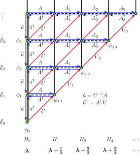
Figure 1: A schematic diagram of the energy levels and the associated Hamiltonian systems together with the definition of the $A$ and $A^{\dagger}$ operators and the ‘creation’ and ‘annihilation’ operators. The parameter set is indicated below each Hamiltonian.

3 Other examples of shape invariant “discrete quantum mechanics”

The other examples of shape invariant “discrete quantum mechanics” are related to a two-parameter deformation of the Hermite polynomial, and two- and three-parameter deformation of the Laguerre polynomial. The Laguerre polynomials are the eigenfunctions of a harmonic oscillator with a centrifugal barrier ($1/x^{2}$ potential). They all belong to the Askey scheme of hypergeometric orthogonal polynomials [3]. Demonstration of the shape invariance and derivation of shift operators and eigenfunctions, etc. go almost parallel with the case of the deformed Hermite polynomials in section 2. We discuss them collectively by adopting an (almost) self-evident notation.

$$\mbox{(i)}\,:\,\mbox{two-parameter deformation of the Hermite polynomial},$$

$$\qquad\mbox{a special case of the {\bf continuous Hahn polynomial}},$$

$$\qquad V(x)=V(x;\bm{\lambda})=(a+ix)(b+ix),$$ (43)

$$\qquad\phi_{0}(x)=\phi_{0}(x;\bm{\lambda})\propto|\Gamma(a+ix)\Gamma(b+ix)|,$$ (44)

$$\qquad\bm{\lambda}=(a,b),\quad{\cal E}_{n}={\cal E}_{n}(\bm{\lambda})={\textstyle\frac{1}{2}}n(n+2a+2b-1),\quad a,b\in\mathbb{R}_{+},$$ (45)

$$\qquad P_{n}(x)=P_{n}^{(\bm{\lambda})}(x)\propto p_{n}(x;a,b,a,b).$$ (46)

$$\mbox{(ii)}\,:\,\mbox{two-parameter deformation of the Laguerre polynomial},$$

$$\qquad\mbox{the {\bf continuous dual Hahn polynomial}},$$

$$\qquad V(x)=V(x;\bm{\lambda})=\frac{(a+ix)(b+ix)(c+ix)}{2ix(2ix+1)},$$ (47)

$$\qquad\phi_{0}(x)=\phi_{0}(x;\bm{\lambda})\propto\left|\frac{\Gamma(a+ix)\Gamma(b+ix)\Gamma(c+ix)}{\Gamma(2ix)}\right|,$$ (48)

$$\qquad\bm{\lambda}=(a,b,c),\quad{\cal E}_{n}={\cal E}_{n}(\bm{\lambda})={\textstyle\frac{1}{2}}n,\quad a,b,c\in\mathbb{R}_{+},$$ (49)

$$\qquad P_{n}(x)=P_{n}^{(\bm{\lambda})}(x)\propto S_{n}(x^{2};a,b,c).$$ (50)

$$\mbox{(iii)}\,:\,\mbox{three-parameter deformation of the Laguerre polynomial},$$

$$\qquad\mbox{the {\bf Wilson polynomial}},$$

$$\qquad V(x)=V(x;\bm{\lambda})=\frac{(a+ix)(b+ix)(c+ix)(d+ix)}{2ix(2ix+1)},$$ (51)

$$\qquad\phi_{0}(x)=\phi_{0}(x;\bm{\lambda})\propto\left|\frac{\Gamma(a+ix)\Gamma(b+ix)\Gamma(c+ix)\Gamma(d+ix)}{\Gamma(2ix)}\right|,$$ (52)

$$\qquad\bm{\lambda}=(a,b,c,d),\;{\cal E}_{n}={\cal E}_{n}(\bm{\lambda})={\textstyle\frac{1}{2}}n(n+a+b+c+d-1),\;a,b,c,d\in\mathbb{R}_{+},$$ (53)

$$\qquad P_{n}(x)=P_{n}^{(\bm{\lambda})}(x)\propto W_{n}(x^{2};a,b,c,d).$$ (54)

For space reasons we write the ground state wavefunction in terms of the absolute value symbol as in (44) which should read

$$|\Gamma(a+ix)\Gamma(b+ix)|=\sqrt{\Gamma(a+ix)\Gamma(b+ix)\Gamma(a-ix)\Gamma(b-ix)}$$

as in (8).

Factorised Hamiltonian

Factorisation and consequently the positive semi-definiteness of the generic Hamiltonian hold exactly the same as before:

$$H\stackrel{{\scriptstyle\rm def}}{{=}}{\textstyle\frac{1}{2}}\sqrt{V(x)}\,e^{-i\partial_{x}}\sqrt{V^{*}(x)}+{\textstyle\frac{1}{2}}\sqrt{V^{*}(x)}\,e^{i\partial_{x}}\sqrt{V(x)}-{\textstyle\frac{1}{2}}(V(x)+V^{*}(x)),$$ (55)

$$H=A^{\dagger}A,$$ (56)

$$A=A(x;\bm{\lambda})\stackrel{{\scriptstyle\rm def}}{{=}}\frac{1}{\sqrt{2}}\Bigl{(}e^{-\frac{i}{2}\partial_{x}}\sqrt{V^{*}(x)}-e^{\frac{i}{2}\partial_{x}}\sqrt{V(x)}\Bigr{)},$$ (57)

$$A^{\dagger}=A(x;\bm{\lambda})^{\dagger}\stackrel{{\scriptstyle\rm def}}{{=}}\frac{1}{\sqrt{2}}\Bigl{(}\sqrt{V(x)}\,e^{-\frac{i}{2}\partial_{x}}-\sqrt{V^{*}(x)}\,e^{\frac{i}{2}\partial_{x}}\Bigr{)}.$$ (58)

Here $\bm{\lambda}$ denotes the (set of) parameters. The ground state $\phi_{0}$ is annihilated by $A$:

$$A\phi_{0}(x)=0\quad\Longrightarrow H\phi_{0}(x)=0,\quad\mathcal{E}_{0}=0.$$ (59)

Verification of the ground state wavefunction (44) for (i), (48) for (ii) and (52) for (iii) is straightforward. The similarity transformed Hamiltonian $\tilde{H}=\phi_{0}^{-1}\circ H\circ\phi_{0}$, (11) determines the other eigenfunctions of the Hamiltonian in the form $\phi_{n}(x)\propto P_{n}(x)\phi_{0}(x)$, $\tilde{H}P_{n}=\mathcal{E}_{n}P_{n}$ (10). They are the difference equation of the form

$$V(x)P_{n}(x-i)+V^{*}(x)P_{n}(x+i)-(V(x)+V^{*}(x))P_{n}(x)=2\mathcal{E}_{n}P_{n}(x).$$ (60)

Explicitly they read for the three cases listed above:

(i) $$: (a+ix)(b+ix)P_{n}(x-i)+(a-ix)(b-ix)P_{n}(x+i)$$ (61)

$$=2(ab-x^{2}+\mathcal{E}_{n})P_{n}(x).$$

(ii) $$: (a+ix)(b+ix)(c+ix)(2ix-1)P_{n}(x-i)+$$ (62)

$$(a-ix)(b-ix)(c-ix)(2ix+1)P_{n}(x+i)$$

$$=-2ix\left[(ab+ac+bc-2abc+2(a+b+c)x^{2}-x^{2}+2(4x^{2}+1)\mathcal{E}_{n}\right]P_{n}(x).$$

(iii) $$: (a+ix)(b+ix)(c+ix)(d+ix)(2ix-1)P_{n}(x-i)+$$ (63)

$$(a-ix)(b-ix)(c-ix)(d-ix)(2ix+1)P_{n}(x+i)$$

$$=-2ix\left[(abc+abd+acd+bcd-2abcd+2(ab+ac+ad+bc+bd+cd)x^{2}\right.$$

$$\qquad\qquad\left.-(a+b+c+d)x^{2}-2x^{4}+2(4x^{2}+1)\mathcal{E}_{n}\right]P_{n}(x).$$

They admit a degree $n$ polynomial solution in $x$ for (i), and in $x^{2}$ for (ii) and (iii). By comparing the coefficients of the leading degree, one obtains the energy eigenvalues $\mathcal{E}_{n}$ (45), (49), (53). The solutions form orthogonal polynomials satisfying three term recurrence, which will not be shown here, see [3].

The corresponding factorisation of $\tilde{H}$,

$$\tilde{H}=BC,\quad C={\textstyle\frac{i}{2}}(e^{-\frac{i}{2}\partial_{x}}-e^{\frac{i}{2}\partial_{x}}),\quad B=-i(V(x)e^{-\frac{i}{2}\partial_{x}}-V^{*}(x)e^{\frac{i}{2}\partial_{x}}),$$ (64)

provides the forward and backward shift operators of the polynomials. The $C$ operator, corresponding to the $A$ operator, shifts to the right along the isospectral line: $C:P_{n}^{(\bm{\lambda})}(x)\to P_{n-1}^{(\bm{\lambda}+\bm{{\textstyle\frac{1}{2}}})}(x)$ with $\bm{{\textstyle\frac{1}{2}}}=({\textstyle\frac{1}{2}},{\textstyle\frac{1}{2}},\cdots)$. The $B$ operator, corresponding to the $A^{\dagger}$ operator, shifts to the left along the isospectral line: $B:P_{n-1}^{(\bm{\lambda}+\bm{{\textstyle\frac{1}{2}}})}(x)\to P_{n}^{(\bm{\lambda})}(x)$. For each case they are:

$$\mbox{(i)}\,:\,BCp_{n}(x;\bm{\lambda})=\mathcal{E}_{n}p_{n}(x;\bm{\lambda})$$

$$\qquad\Longleftarrow Cp_{n}(x;\bm{\lambda})=(\mathcal{E}_{n}/n)p_{n-1}(x;\bm{\lambda}+\bm{{\textstyle\frac{1}{2}}}),\quad Bp_{n-1}(x;\bm{\lambda}+\bm{{\textstyle\frac{1}{2}}})=np_{n}(x;\bm{\lambda}),$$ (65)

$$\qquad p_{n}(x+{\textstyle\frac{i}{2}};\bm{\lambda})-p_{n}(x-{\textstyle\frac{i}{2}};\bm{\lambda})=i(n+2a+2b-1)p_{n-1}(x;\bm{\lambda}+\bm{{\textstyle\frac{1}{2}}}),$$ (66)

$$\qquad(a-ix)(b-ix)p_{n-1}(x+{\textstyle\frac{i}{2}};\bm{\lambda}+\bm{{\textstyle\frac{1}{2}}})-(a+ix)(b+ix)p_{n-1}(x-{\textstyle\frac{i}{2}};\bm{\lambda}+\bm{{\textstyle\frac{1}{2}}})$$

$$\qquad\quad=-inp_{n}(x;\bm{\lambda}).$$ (67)

$$\mbox{(ii)}\,:\,BCS_{n}(x^{2};\bm{\lambda})=\mathcal{E}_{n}S_{n}(x^{2};\bm{\lambda})$$

$$\qquad\Longleftarrow CS_{n}(x^{2};\bm{\lambda})=-2\mathcal{E}_{n}xS_{n-1}(x^{2};\bm{\lambda}+\bm{{\textstyle\frac{1}{2}}}),\ -2B\,xS_{n-1}(x^{2};\bm{\lambda}+\bm{{\textstyle\frac{1}{2}}})=S_{n}(x^{2};\bm{\lambda}),$$ (68)

$$\qquad S_{n}((x+{\textstyle\frac{i}{2}})^{2};\bm{\lambda})-S_{n}((x-{\textstyle\frac{i}{2}})^{2};\bm{\lambda})=-2inxS_{n-1}(x^{2};\bm{\lambda}+\bm{{\textstyle\frac{1}{2}}}),$$ (69)

$$\qquad(a-ix)(b-ix)(c-ix)S_{n-1}((x+{\textstyle\frac{i}{2}})^{2};\bm{\lambda}+\bm{{\textstyle\frac{1}{2}}})$$

$$\qquad-(a+ix)(b+ix)(c+ix)S_{n-1}((x+{\textstyle\frac{i}{2}})^{2};\bm{\lambda}+\bm{{\textstyle\frac{1}{2}}})$$

$$\qquad\quad=-2ixS_{n}(x^{2};\bm{\lambda}).$$ (70)

$$\mbox{(iii)}\,:\,BCW_{n}(x^{2};\bm{\lambda})=\mathcal{E}_{n}W_{n}(x^{2};\bm{\lambda})$$

$$\qquad\Longleftarrow CW_{n}(x^{2};\bm{\lambda})=-2\mathcal{E}_{n}xW_{n-1}(x^{2};\bm{\lambda}+\bm{{\textstyle\frac{1}{2}}}),\ -2B\,xW_{n-1}(x^{2};\bm{\lambda}+\bm{{\textstyle\frac{1}{2}}})=W_{n}(x^{2};\bm{\lambda}),$$ (71)

$$\qquad W_{n}((x+{\textstyle\frac{i}{2}})^{2};\bm{\lambda})-W_{n}((x-{\textstyle\frac{i}{2}})^{2};\bm{\lambda})$$

$$\qquad\quad=-2in(n+a+b+c+d-1)\,xW_{n-1}(x^{2};\bm{\lambda}+\bm{{\textstyle\frac{1}{2}}}),$$ (72)

$$\qquad(a-ix)(b-ix)(c-ix)(d-ix)W_{n-1}((x+{\textstyle\frac{i}{2}})^{2};\bm{\lambda}+\bm{{\textstyle\frac{1}{2}}})$$

$$\qquad-(a+ix)(b+ix)(c+ix)(d+ix)W_{n-1}((x+{\textstyle\frac{i}{2}})^{2};\bm{\lambda}+\bm{{\textstyle\frac{1}{2}}})$$

$$\qquad\quad=-2ixW_{n}(x^{2};\bm{\lambda}).$$ (73)

Shape Invariance

For shape invariance, we first need to find the operators $A_{1}$, $A_{1}^{\dagger}$ and a real constant $\mathcal{E}_{1}$ satisfying

$$H_{1}=AA^{\dagger}=A_{1}^{\dagger}A_{1}+{\cal E}_{1},$$ (74)

$$A_{1}=A_{1}(x;\bm{\lambda})\stackrel{{\scriptstyle\rm def}}{{=}}\frac{1}{\sqrt{2}}\Bigl{(}e^{-\frac{i}{2}\partial_{x}}\sqrt{V_{1}^{*}(x)}-e^{\frac{i}{2}\partial_{x}}\sqrt{V_{1}(x)}\Bigr{)},$$ (75)

$$A_{1}^{\dagger}=A_{1}(x;\bm{\lambda})^{\dagger}\stackrel{{\scriptstyle\rm def}}{{=}}\frac{1}{\sqrt{2}}\Bigl{(}\sqrt{V_{1}(x)}\,e^{-\frac{i}{2}\partial_{x}}-\sqrt{V_{1}^{*}(x)}\,e^{\frac{i}{2}\partial_{x}}\Bigr{)}.$$ (76)

In other words, given $V(x)=V(x;\bm{\lambda})$, find a new potential $V_{1}(x)=V_{1}(x;\bm{\lambda})$ satisfying

$$V_{1}^{*}(x-i)V_{1}(x)=V^{*}(x-{\textstyle\frac{i}{2}})V(x-{\textstyle\frac{i}{2}}),$$ (77)

$$V_{1}(x)+V_{1}^{*}(x)=V(x+{\textstyle\frac{i}{2}})+V^{*}(x-{\textstyle\frac{i}{2}})+2{\cal E}_{1}.$$ (78)

If $V_{1}$ has the same form as $V$ with a shifted set of parameters $\bm{\lambda}^{\prime}$,

$$V_{1}(x;\bm{\lambda})=V(x;\bm{\lambda}^{\prime}),$$ (79)

it is shape invariant. Suppose $V_{1}$ has the form $V_{1}(x)=V(x-{\textstyle\frac{i}{2}})g(x)$, the above conditions (77), (78) get slightly simplified:

$$g^{*}(x-i)g(x)=1,$$ (80)

$$V(x-{\textstyle\frac{i}{2}})g(x)+V^{*}(x+{\textstyle\frac{i}{2}})g^{*}(x)=V(x+{\textstyle\frac{i}{2}})+V^{*}(x-{\textstyle\frac{i}{2}})+2{\cal E}_{1}.$$ (81)

The following choice satisfies the above conditions (80), (80) for the three cases (44)–(54):

(i) $$: g(x)=1,\quad\mathcal{E}_{1}(\bm{\lambda})=a+b,$$ (83)

$$V_{1}(x;\bm{\lambda})=V(x-{\textstyle\frac{i}{2}};a,b)=V(x;a+{\textstyle\frac{1}{2}},b+{\textstyle\frac{1}{2}}).$$

(ii) $$: g(x)=\frac{2ix+2}{2ix},\quad\mathcal{E}_{1}(\bm{\lambda})={\textstyle\frac{1}{2}},$$ (85)

$$V_{1}(x;\bm{\lambda})=V(x-{\textstyle\frac{i}{2}};a,b,c)g(x)=V(x;a+{\textstyle\frac{1}{2}},b+{\textstyle\frac{1}{2}},c+{\textstyle\frac{1}{2}}).$$

(iii) $$: g(x)=\frac{2ix+2}{2ix},\quad\mathcal{E}_{1}(\bm{\lambda})={\textstyle\frac{1}{2}}(a+b+c+d),$$ (87)

$$V_{1}(x;\bm{\lambda})=V(x-{\textstyle\frac{i}{2}};a,b,c,d)g(x)=V(x;a+{\textstyle\frac{1}{2}},b+{\textstyle\frac{1}{2}},c+{\textstyle\frac{1}{2}},d+{\textstyle\frac{1}{2}}).$$

With $\bm{{\textstyle\frac{1}{2}}}=({\textstyle\frac{1}{2}},{\textstyle\frac{1}{2}},\cdots)$, we have collectively

$$V_{1}(x;\bm{\lambda})=V(x;\bm{\lambda}+\bm{{\textstyle\frac{1}{2}}}),\ A_{1}(x;\bm{\lambda})=A(x;\bm{\lambda}+\bm{{\textstyle\frac{1}{2}}}),\ H_{1}(x;\bm{\lambda})=H(x;\bm{\lambda}+\bm{{\textstyle\frac{1}{2}}})+{\cal E}_{1}(\bm{\lambda}).$$ (88)

Starting from $V_{0}=V$, $H_{0}=H$, $\phi_{0,n}=\phi_{n}$, let us define $V_{s}$, $H_{s}$, $\phi_{s,n}$ ($n\geq s\geq 0$) step by step:

$$V_{s+1}(x;\bm{\lambda})\stackrel{{\scriptstyle\rm def}}{{=}}V_{s}(x;\bm{\lambda}+\bm{{\textstyle\frac{1}{2}}}),$$ (89)

$$H_{s+1}(x;\bm{\lambda})\stackrel{{\scriptstyle\rm def}}{{=}}A_{s}(x;\bm{\lambda})A_{s}(x;\bm{\lambda})^{\dagger}+{\cal E}_{s}(\bm{\lambda}),$$ (90)

$$\phi_{s+1,n}(x;\bm{\lambda})\stackrel{{\scriptstyle\rm def}}{{=}}A_{s}(x;\bm{\lambda})\phi_{s,n}(x;\bm{\lambda}),$$ (91)

$${\cal E}_{s}(\bm{\lambda})={\cal E}_{s-1}(\bm{\lambda})+{\cal E}_{1}(\bm{\lambda}+\bm{(s-1)/{2}}).$$ (92)

Here $A_{s}$, $A_{s}^{\dagger}$ are defined by

$$A_{s}(x;\bm{\lambda})\stackrel{{\scriptstyle\rm def}}{{=}}\frac{1}{\sqrt{2}}\Bigl{(}e^{-\frac{i}{2}\partial_{x}}\sqrt{V_{s}^{*}(x;\bm{\lambda})}-e^{\frac{i}{2}\partial_{x}}\sqrt{V_{s}(x;\bm{\lambda})}\Bigr{)},$$ (93)

$$A_{s}(x;\bm{\lambda})^{\dagger}\stackrel{{\scriptstyle\rm def}}{{=}}\frac{1}{\sqrt{2}}\Bigl{(}\sqrt{V_{s}(x;\bm{\lambda})}\,e^{-\frac{i}{2}\partial_{x}}-\sqrt{V_{s}^{*}(x;\bm{\lambda})}\,e^{\frac{i}{2}\partial_{x}}\Bigr{)}.$$ (94)

As a consequence of the shape invariance, we obtain for $n\geq s\geq 0$:

$$V_{s}(x;\bm{\lambda})=V(x;\bm{\lambda}+\bm{{\textstyle\frac{s}{2}}}),$$ (95)

$$A_{s}(x;\bm{\lambda})=A(x;\bm{\lambda}+\bm{{\textstyle\frac{s}{2}}}),\quad A_{s}(x;\bm{\lambda})^{\dagger}=A(x;\bm{\lambda}+\bm{{\textstyle\frac{s}{2}}})^{\dagger},$$ (96)

$$H_{s}(x;\bm{\lambda})=A_{s}(x;\bm{\lambda})^{\dagger}A_{s}(x;\bm{\lambda})+{\cal E}_{s}(\bm{\lambda}),$$ (97)

$$H_{s}(x;\bm{\lambda})\phi_{s,n}(x;\bm{\lambda})={\cal E}_{n}(\bm{\lambda})\phi_{s,n}(x;\bm{\lambda}),$$ (98)

$$A_{s}(x;\bm{\lambda})\phi_{s,s}(x;\bm{\lambda})=0,$$ (99)

$$A_{s}(x;\bm{\lambda})^{\dagger}\phi_{s+1,n}(x;\bm{\lambda})=({\cal E}_{n}(\bm{\lambda})-{\cal E}_{s}(\bm{\lambda}))\phi_{s,n}(x;\bm{\lambda}).$$ (100)

The eigenfunction $\phi_{s,n}$ has $n-s$ nodes, or the corresponding polynomial is of degree $n-s$ in $x$ for (i), and in $x^{2}$ for (ii) and (iii). In the latter case, the zeros on a half line, say $x\geq 0$, count as the nodes.

From these we obtain formulas

$$\phi_{s,n}(x;\bm{\lambda})=A_{s-1}(x;\bm{\lambda})\cdots A_{1}(x;\bm{\lambda})A_{0}(x;\bm{\lambda})\phi_{n}(x;\bm{\lambda}),$$ (101)

$$\phi_{n}(x;\bm{\lambda})=\frac{A_{0}(x;\bm{\lambda})^{\dagger}}{{\cal E}_{n}(\bm{\lambda})-{\cal E}_{0}(\bm{\lambda})}\,\frac{A_{1}(x;\bm{\lambda})^{\dagger}}{{\cal E}_{n}(\bm{\lambda})-{\cal E}_{1}(\bm{\lambda})}\cdots\frac{A_{n-1}(x;\bm{\lambda})^{\dagger}}{{\cal E}_{n}(\bm{\lambda})-{\cal E}_{n-1}(\bm{\lambda})}\,\phi_{n,n}(x;\bm{\lambda}),$$ (102)

corresponding to (34) and (42) discussed in section 2. The former (101) gives the eigenfunction $\phi_{s,n}$ of the $s$-th Hamiltonian $H_{s}$ along the isospectral line with energy $\mathcal{E}_{n}$, starting from $\phi_{n}$ of the original Hamiltonian $H$ by repeated application of the $A$ operators. The latter (102), on the other hand, expresses the $n$-th eigenfunction $\phi_{n}$ of the original Hamiltonian, starting from the explicitly known ground state $\phi_{n,n}$ of the $n$-th Hamiltonian $H_{n}$ by repeated application of the $A^{\dagger}$ operators. The latter formula (102), a simple generalisation of the well-known formula for the harmonic oscillator $|n\rangle\propto(a^{\dagger})^{n}|0\rangle$, could also be understood as the generic form of the Rodrigue’s formula for the orthogonal polynomials.

In order to define the annihilation and creation operators, let us introduce normalised basis $\{\hat{\phi}_{s,n}\}_{n\geq s}$ for each Hamiltonian $H_{s}$. Ordinarily, the phase of each element of an orthonormal basis could be completely arbitrary. In the present case, however, the eigenfunctions are orthogonal polynomials. That is, they are real and the relations among different degree members are governed by the three term recurrence relations. So the phases of $\{\hat{\phi}_{s,n}\}_{n\geq s}$ are fixed. Let us introduce a unitary (in fact an orthogonal) operator $U_{s}$ mapping the $s$-th orthonormal basis $\{\hat{\phi}_{s,n}\}_{n\geq s}$ to the $(s+1)$-th $\{\hat{\phi}_{s+1,n}\}_{n\geq s+1}$ (see Fig. 1 and for example [16, 17]):

$$U_{s}\hat{\phi}_{s,n}=\hat{\phi}_{s+1,n+1},\quad U_{s}^{\dagger}\hat{\phi}_{s+1,n+1}=\hat{\phi}_{s,n}.$$ (103)

We denote that $U_{0}=U$. Roughly speaking $U$ increases the parameters from $\bm{\lambda}$ to $\bm{\lambda}+\bm{{\textstyle\frac{1}{2}}}$:

$$U:P_{n}^{(\bm{\lambda})}(x)\to P_{n}^{(\bm{\lambda}+\bm{{\textstyle\frac{1}{2}}})}(x),\quad U^{\dagger}:P_{n}^{(\bm{\lambda}+\bm{{\textstyle\frac{1}{2}}})}(x)\to P_{n}^{(\bm{\lambda})}(x).$$

Let us introduce an annihilation $\tilde{a}$ and a creation operator $\tilde{a}^{\dagger}$ for the Hamiltonian $H$ as follows:

$$\tilde{a}=\tilde{a}(x;\bm{\lambda})\stackrel{{\scriptstyle\rm def}}{{=}}U^{\dagger}A(x;\bm{\lambda}),\quad\tilde{a}^{\dagger}=\tilde{a}(x;\bm{\lambda})^{\dagger}\stackrel{{\scriptstyle\rm def}}{{=}}A(x;\bm{\lambda})^{\dagger}U.$$ (104)

It is straightforward to derive

$$H=\tilde{a}^{\dagger}\tilde{a},$$ (105)

$$[\tilde{a},\tilde{a}^{\dagger}]\hat{\phi}_{n}(x;\lambda)=({\cal E}_{n+1}(\bm{\lambda})-{\cal E}_{n}(\bm{\lambda}))\hat{\phi}_{n}(x;\lambda).$$ (106)

For the harmonic oscillator (1) $U=$id. and we recover the known result. For the linear spectrum $\mathcal{E}_{n}=n,n/2$ of the deformed Hermite polynomial (3) and the two parameter deformation of the Laguerre polynomial (47)–(50), $\tilde{a}$ and $\tilde{a}^{\dagger}$ have the same (up to rescaling) commutation relations as those of the harmonic oscillator. Essentially the same arguments and results hold for the annihilation $\tilde{a}_{s}=U_{s}^{\dagger}A_{s}(x;\bm{\lambda})$ and the creation operator $\tilde{a}_{s}^{\dagger}=A_{s}(x;\bm{\lambda})U_{s}$ for the Hamiltonian $H_{s}$.

4 Dynamical Background

Here we will show briefly a logical (dynamical) path that led to the shape invariant difference equations introduced in section 2. The equilibrium position of an $n$-particle A-type Calogero system is determined by

$$\sum_{k=1\atop k\neq j}^{n}\frac{1}{x_{j}-x_{k}}=x_{j}\,,\quad j=1,\ldots,n,$$ (107)

after adjustment of the coupling constants and rescaling of the variables [8, 9]. They describe the zeros of the Hermite polynomial, since $H_{n}(x)\stackrel{{\scriptstyle\rm def}}{{=}}2^{n}\prod_{j=1}^{n}(x-x_{j})$ satisfies the differential equation

$$H_{n}^{{}^{\prime\prime}}(x)-2xH_{n}^{\prime}(x)+2nH_{n}(x)=0$$ (108)

and the three term recurrence [9] $n\geq 0$,

$$H_{n+1}(x)-2xH_{n}(x)+2nH_{n-1}(x)=0,\quad H_{0}=1,\quad H_{-1}=0.$$ (109)

The equilibrium position of an $n$-particle A-type van Diejen system (or the rational R-S system with a linear confining potential) is determined by

$$\prod_{k=1\atop k\neq j}^{n}\frac{x_{j}-x_{k}-i\sqrt{\delta}}{x_{j}-x_{k}+i\sqrt{\delta}}=\frac{1-i\sqrt{\delta}\,x_{j}}{1+i\sqrt{\delta}\,x_{j}}\,,\quad j=1,\ldots,n,$$ (110)

after adjustment of the coupling constants and rescaling of the variables [11]. The corresponding deformed polynomial $H_{n}(x,\delta)\stackrel{{\scriptstyle\rm def}}{{=}}2^{n}\prod_{j=1}^{n}(x-x_{j})$ satisfies the difference equation

$$\Bigl{(}x+\frac{i}{\sqrt{\delta}}\Bigr{)}H_{n}(x+i\sqrt{\delta},\delta)-\Bigl{(}x-\frac{i}{\sqrt{\delta}}\Bigr{)}H_{n}(x-i\sqrt{\delta},\delta)=\frac{2i}{\sqrt{\delta}}(1+n\delta\,)H_{n}(x,\delta),$$ (111)

and the three term recurrence [11] $n\geq 0$,

$$H_{n+1}(x,\delta)-2xH_{n}(x,\delta)+\Bigl{(}2n+n(n-1)\delta\Bigr{)}H_{n-1}(x,\delta)=0,\quad H_{0}=1,\quad H_{-1}=0.$$ (112)

It is elementary to show that (110), (111), (112) reduce to (107), (108), (109) in the zero deformation limit $\delta\to 0$; $\lim_{\delta\to 0}H_{n}(x,\delta)=H_{n}(x)$. The relationship between the deformed Hermite polynomial and the special case of the Meixner-Pollaczek polynomial discussed in section 2 is

$$H_{n}(x,\delta)=n!\sqrt{\delta}^{\,n}P_{n}^{(\frac{1}{\delta})}\Bigl{(}\frac{x}{\sqrt{\delta}}\,;\frac{\pi}{2}\Bigr{)}.$$ (113)

It is instructive to write down the classical Hamiltonian of the $n$-particle A-type van Diejen system

$$H(p,q)=\sum_{j=1}^{n}\left(\cosh p_{j}\,\sqrt{V_{j}(q)\,{V}_{j}^{*}(q)}-\frac{1}{2}\Bigl{(}V_{j}(q)+{V}_{j}^{*}(q)\Bigr{)}\right),$$ (114)

$$V_{j}(q)=\left(1+\frac{iq_{j}}{a}\right)\prod_{k=1\atop k\neq j}^{n}\left(1-\frac{ig}{q_{j}-q_{k}}\right),$$ (115)

in which $a$ and $g$ are coupling constants. In fact, the Hamiltonian (3) is the single particle ($n=1$) case with $p_{j}=-i{\partial}/{\partial q_{j}}$ and proper ordering. We refer to [11] for similar orientation of the dynamical systems introduced in section 3.

5 Comments and Discussion

Several examples of shape invariant difference equations are discussed in some detail. They are related to deformation of the harmonic oscillator without/with a centrifugal potential and their eigenfunctions are deformed Hermite and Laguerre polynomials belonging to the Askey-scheme of hypergeometric orthogonal polynomials. They arise in the problems of determining the equilibrium positions of the Ruijsenaars-Schneider-van Diejen systems, which are integrable deformation of the celebrated Calogero-Sutherland systems of exactly solvable multi-particle quantum mechanics. Here we have treated rational potentials $V(x)$ only. Obviously the method works for a wider range of potentials, the trigonometric, hyperbolic, elliptic, etc. We have not discussed the shape invariance of the discrete systems corresponding to the equilibria of the trigonometric Ruijsenaars-Schneider systems. These have various kinds of deformed Jacobi polynomials as eigenfunctions [11]. We will report on this subject elsewhere.

In the literature, shape invariance is discussed almost always within the context of ‘supersymmetric quantum mechanics’[1]. We presume that this might be the psychological barrier for considering the shape invariance in discrete quantum mechanics, or shape invariant difference equations. As is well-known, supersymmetry is the ‘square root’ of the space-time symmetry, say the Poincaré symmetry, which is usually lost if the space-time is discretised….. In fact, it is important to realise that main results of ‘supersymmetric quantum mechanics’ are already contained in Crum’s theorem without supersymmetry or shape invariance. Among them are: the existence of associated isospectral Hamiltonians $H_{1}$, …, $H_{s}$, …, as many as the number of discrete levels of $H_{0}$ and the formulas of their eigenfunctions. For example, $\phi_{s,n}$ of $H_{s}$ with the eigenvalue $\mathcal{E}_{n}$ is expressed in terms of the eigenfunctions $\phi_{0}$, $\phi_{1}$,…, $\phi_{s-1}$, $\phi_{n}$ of $H_{0}$ (Fig. 1):

$$\phi_{s,n}=\frac{\mathcal{W}_{s,n}}{\mathcal{W}_{s}},\quad n\geq s\geq 1,$$ (116)

$$\mathcal{W}_{s}=\mathcal{W}[\phi_{0},\ldots,\phi_{s-1}],\quad\mathcal{W}_{s,n}=\mathcal{W}[\phi_{0},\ldots,\phi_{s-1},\phi_{n}].$$ (117)

Here the Wronskian $\mathcal{W}$ is defined as usual $\mathcal{W}[f_{1},\ldots,f_{n}]=\det\left(f_{j}^{(i-1)}\right)_{1\leq i,j\leq n}$. This formula, translated in the discrete dynamics context, corresponds to (101).

We do believe dynamical (Hamiltonian) interpretation of discrete quantum systems (difference equations) would be useful and fruitful. One of our starting points, equations determining a certain equilibrium, eg. (110), are called Bethe ansatz like equations. The present problems could be considered as those of finding associated polynomial solutions of Bethe ansatz like equations. They occur in many branches of theoretical physics, for example, the quasi-exactly solvable single and multi-particle quantum systems [18] on top of the well-known integrable spin chains [19].

References

• [1] L. E. Gendenshtein, “Derivation of exact spectra of the Schrodinger equation by means of supersymmetry,” JETP Lett.  38 (1983) 356-359.
• [2] G. E. Andrews, R. Askey and R. Roy, “Special Functions”, Encyclopedia of mathematics and its applications, Cambridge, (1999).
• [3] R.  Koekoek and R.  F. Swarttouw, “The Askey-scheme of hypergeometric orthogonal polynomials and its $q$-analogue”, math.CA/9602214.
• [4] N. A.  Atakishiyev and S. K. Suslov, “The Hahn and Meixner polynomials of an imaginary argument and some of their applications”, J. Phys. A18 (1985) 1583-1696; “Difference analogs of the harmonic oscillator”, Theor. Math. Phys. 85 (1990) 1055-1062.
• [5] C. M.  Bender, L. R. Mead and S. S. Pinsky, “Resolution of operator-ordering problem by the method of finite elements”, Phys. Rev. Lett. 56 (1986) 2445-2448; “Continuous Hahn polynomials and the Heisenberg algebra”, J. Math. Phys. 28 (1987) 509-513; T.  H.  Koornwinder, “Meixner-Pollaczek polynomials and the Heisenberg algebra”, J. Math. Phys. 30 (1989) 767-769.
• [6] F. Calogero, “Solution of the one-dimensional $N$-body problem with quadratic and/or inversely quadratic pair potentials”, J. Math. Phys. 12 (1971) 419-436; B. Sutherland, “Exact results for a quantum many-body problem in one-dimension. II”, Phys. Rev. A5 (1972) 1372-1376.
• [7] S. N. M Ruijsenaars and H. Schneider, “A New Class Of Integrable Systems And Its Relation To Solitons,” Annals Phys. 170 (1986) 370-405; S. N. M Ruijsenaars, “Complete Integrability of Relativistic Calogero-Moser Systems And Elliptic Function Identities,” Comm. Math. Phys.  110 (1987) 191-213; J. F. van Diejen, “Integrability of difference Calogero-Moser systems”, J. Math. Phys. 35 (1994) 2983-3004; “The relativistic Calogero model in an external field,” solv-int/ 9509002; “Multivariable continuous Hahn and Wilson polynomials related to integrable difference systems”, J. Phys. A28 (1995) L369-L374: “Difference Calogero-Moser systems and finite Toda chains”, J. Math. Phys. 36 (1995) 1299-1323.
• [8] F. Calogero, “On the zeros of the classical polynomials”, Lett. Nuovo Cim. 19 (1977) 505-507; “Equilibrium configuration of one-dimensional many-body problems with quadratic and inverse quadratic pair potentials”, Lett. Nuovo Cim. 22 (1977) 251-253.
• [9] T. Stieltjes, “Sur quelques théorèmes d’Algèbre”, Compt. Rend. 100 (1885) 439-440; “Sur les polynômes de Jacobi”, Compt. Rend. 100 (1885) 620-622; G. Szegö, “Orthogonal polynomials”, Amer. Math. Soc. New York (1939).
• [10] E. Corrigan and R. Sasaki, “Quantum vs Classical Integrability in Calogero-Moser Systems”, J. Phys. A35 (2002) 7017-7062; S. Odake and R. Sasaki, “Polynomials Associated with Equilibrium Positions in Calogero-Moser Systems,” J. Phys. A35 (2002) 8283-8314.
• [11] O. Ragnisco and R. Sasaki, “Quantum vs Classical Integrability in Ruijsenaars-Schneider Systems,” J. Phys. A37 (2004) 469-479; S. Odake and R. Sasaki, “Equilibria of ‘Discrete’ Integrable Systems and Deformations of Classical Polynomials”, hep-th/0407155.
• [12] L. Infeld and T. E. Hull, “The factorization method,” Rev. Mod. Phys.  23 (1951) 21-68.
• [13] M. M. Crum, “Associated Sturm-Liouville systems”, Quart. J. Math. Oxford Ser. (2) 6 (1955) 121-127, physics/9908019.
• [14] See, for example, a review: F. Cooper, A. Khare and U. Sukhatme, “Supersymmetry and quantum mechanics,” Phys. Rept.  251 (1995) 267-385.
• [15] See for example: W. Miller Jr., “Lie theory and difference equations. I”, J. Math. Anal. Appl. 28 (1969) 383-399; V. Spiridonov, L. Vinet and A. Zhedanov, “Spectral transformations, self-similar reductions and orthogonal polynomials”, J. Phys. A30 (1997), 7621-7637; G.  Bangerezako , “The factorization method for the Askey-Wilson polynomials”, J. Comp. Appl. Math. 107 (1999) 219-232; G. Bangerezako and M. N.  Hounkonnou, “The transformation of polynomial eigenfunctions of linear second-order difference operators: a special case of Meixner polynomials”, J. Phys. A34 (2001) 5653-5666.
• [16] V. Spiridonov, L. Vinet and A. Zhedanov, “Difference Schrodinger operators with linear and exponential discrete spectra,” Lett. Math. Phys.  29 (1993) 63.
• [17] A.  H.  El Kinani and M.  Daoud “Generalized coherent and intelligent states for exact solvable quantum systems” J. Math. Phys. 43 (2002) 714-733.
• [18] D.  Mayer, A. Ushveridze and Z. Walczak, “ On time-dependent quasi-exactly solvable models”, Mod. Phys. Lett. A15 (2000) 1243-1252; R. Sasaki and K. Takasaki, “Quantum Inozemtsev model, quasi-exact solvability and N-fold supersymmetry,” J. Phys.  A34 (2001) 9533-9553, [Erratum-ibid.  A34 (2001) 10335].
• [19] M. E.  H.  Ismail, S.  S.  Lin and S.  S.  Roan, “Bethe Ansatz Equations of XXZ Model and q-Sturm-Liouville Problems”, math-ph/0407033.