CPTH RR 057.0904 LPT-ORSAY 04/82 ROM2F-04/28 hep-th/0410101 On tadpoles and vacuum redefinitions in String Theory

Tadpoles accompany, in one form or another, all attempts to realize supersymmetry breaking in String Theory, making the present constructions at best incomplete. Whereas these tadpoles are typically large, a closer look at the problem from a perturbative viewpoint has the potential of illuminating at least some of its qualitative features in String Theory. A possible scheme to this effect was proposed long ago by Fischler and Susskind, but incorporating background redefinitions in string amplitudes in a systematic fashion has long proved very difficult. In the first part of this paper, drawing from field theory examples, we thus begin to explore what one can learn by working perturbatively in a “wrong” vacuum. While unnatural in Field Theory, this procedure presents evident advantages in String Theory, whose definition in curved backgrounds is mostly beyond reach at the present time. At the field theory level, we also identify and characterize some special choices of vacua where tadpole resummations terminate after a few contributions. In the second part we present a notable example where vacuum redefinitions can be dealt with to some extent at the full string level, providing some evidence for a new link between IIB and 0B orientifolds. We finally show that $NS$-$NS$ tadpoles do not manifest themselves to lowest order in certain classes of string constructions with broken supersymmetry and parallel branes, including brane-antibrane pairs and brane supersymmetry breaking models, that therefore have UV finite threshold corrections at one loop.

1. Introduction

In String Theory the breaking of supersymmetry is generally accompanied by the emergence of $NS$-$NS$ tadpoles, one-point functions for certain bosonic fields to go into the vacuum. Whereas their $R-R$ counterparts signal inconsistencies of the field equations or quantum anomalies [1], these tadpoles are commonly regarded as mere signals of modifications of the background. Still, for a variety of conceptual and technical reasons, they are the key obstacle to a satisfactory picture of supersymmetry breaking, an essential step to establish a proper connection with Particle Physics. Their presence introduces infrared divergences in string amplitudes: while these have long been associated to the need for background redefinitions [2], it has proved essentially impossible to deal with them in a full-fledged string setting. For one matter, in a theory of gravity these redefinitions affect the background space time, and the limited technology presently available for quantizing strings in curved spaces makes it very difficult to implement them in practice.

This paper is devoted to exploring what can possibly be learnt if one insists on working in a Minkowski background, that greatly simplifies string amplitudes, even when tadpoles arise. This choice may appear contradictory since, from the world-sheet viewpoint, the emergence of tadpoles signals that the Minkowski background becomes a “wrong vacuum”. Indeed, loop and perturbative expansions cease in this case to be equivalent, while the leading infrared contributions need suitable resummations. In addition, in String Theory $NS$-$NS$ tadpoles are typically large, so that a perturbative approach is not fully justified. While we are well aware of these difficulties, we believe that this approach has the advantage of making a concrete string analysis possible, if only of qualitative value in the general case, and has the potential of providing good insights into the nature of this crucial problem. A major motivation for us is that the contributions to the vacuum energy from Riemann surfaces with arbitrary numbers of boundaries, where $NS$-$NS$ tadpoles can emerge already at the disk level, play a key role in orientifold models [3]. This is particularly evident for the mechanism of brane supersymmetry breaking [4, 5], where the simultaneous presence of branes and antibranes of different types, required by the simultaneous presence of $O_{+}$ and $O_{-}$ planes, and possibly of additional brane-antibrane systems [4, 5, 6], is generically accompanied by $NS$-$NS$ tadpoles that first emerge at the disk and projective disk level. Similar considerations apply to non-supersymmetric intersecting brane models [7], and the three mechanisms mentioned above have a common feature: in all of them supersymmetry is preserved, to lowest order, in the closed sector, while it is broken in the open (brane) sector. However, problems of this type are ubiquitous also in closed-string constructions [8] based on the Scherk-Schwarz mechanism [9], where their emergence is only postponed to the torus amplitude.

To give a flavor of the difficulties one faces, let us begin by considering models where only a tadpole $\Delta^{(0)}$ for the dilaton $\varphi$ is present. The resulting higher-genus contributions to the vacuum energy are then plagued with infrared (IR) divergences originating from dilaton propagators that go into the vacuum at zero momentum, so that the leading (IR dominated) contributions to the vacuum energy have the form

$$\Lambda_{0} = e^{-\varphi}\ \Delta^{(0)}+\frac{1}{2}\,\Delta^{(m)}\,\left(i\;{\cal D}_{0}^{mn}\right)\,\Delta^{(n)}+\frac{1}{2}\,e^{\varphi}\,\Delta^{(m)}\,\left(i\;{\cal D}_{0}^{mn}\right)\,\Sigma^{np}\,\left(i\;{\cal D}_{0}^{pq}\right)\,\Delta^{(q)}+\cdots$$ (1.1)

$$= e^{-\varphi}\ \Delta^{(0)}\ +\ \frac{1}{2}\,\Delta\,[\;1-e^{\varphi}\left(i\;{\cal D}_{0}\right)\Sigma\;]^{-1}\left(i\;{\cal D}_{0}\right)\,\Delta\ +\cdots\ .$$

Eq. (1.1) contains in general contributions from the dilaton and from its massive Kaluza-Klein recurrences, implicit in its second form, where they are taken to fill a vector $\Delta$ whose first component is the dilaton tadpole $\Delta^{(0)}$. Moreover,

$$\langle m|{\cal D}_{0}(p^{2})|n\rangle\ \equiv\ {\cal D}_{0}^{(mn)}(p^{2})=\delta^{mn}{\cal D}_{0}^{(mm)}(p^{2})$$ (1.2)

and

$$\langle m|\Sigma_{0}(p^{2})|n\rangle\ \equiv\ \Sigma^{(mn)}(p^{2})$$ (1.3)

denote the sphere-level propagator of a dilaton recurrence of mass $m$ and the matrix of two-point functions for dilaton recurrences of masses $m$ and $n$ on the disk. They are both evaluated at zero momentum in (1.1), where the first term is the disk (one-boundary) contribution, the second is the cylinder (two-boundary) contribution, the third is the genus 3/2 (three-boundary) contribution, and so on. The resummation in the last line of (1.1) is thus the string analogue of the more familiar Dyson propagator resummation in Field Theory,

$$-i\;{\cal D}^{-1}(p^{2})\ =\ -i\;{\cal D}_{0}^{-1}(p^{2})-e^{\varphi}\,\Sigma(p^{2})\ ,$$ (1.4)

where in our conventions the self-energy $\Sigma(p^{2})$ does not include the string coupling in its definition. Even if the individual terms in (1.1) are IR divergent, the resummed expression is in principle perfectly well defined at zero momentum, and yields

$$\Lambda_{0}=e^{-\varphi}\Delta^{(0)}\,-\,\frac{1}{2}\,e^{-\varphi}\,\Delta^{(0)}\,\Sigma^{-1\ (00)}\,\Delta^{(0)}\,+\,\frac{1}{2}\sum_{m,n\neq 0}\!\Delta^{(m)}\left([1-e^{\varphi}\left(i\;{\cal D}_{0}\right)\Sigma]^{-1}\left(i\;{\cal D}_{0}\right)\right)^{mn}\Delta^{(n)}\ .$$ (1.5)

In addition, the soft dilaton theorem implies that

$$e^{\varphi}\,\Sigma^{(00)}=\frac{\partial}{\partial\varphi}\ \left(e^{\varphi}\,\Delta^{(0)}\right)\ ,$$ (1.6)

so that the first two contributions cancel one another, up to a relative factor of two. This is indeed a rather compact result, but here we are describing for simplicity only a partial resummation, that does not take into account higher-point functions: a full resummation is in general far more complicated to deal with, and therefore it is essential to identify possible simplifications of the procedure.

A lesson we shall try to provide in this work, via a number of toy examples based on model field theories meant to shed light on different features of the realistic string setting, is that when a theory is expanded around a “wrong” vacuum, the vacuum energy is typically driven to its value at a nearby extremum (not necessarily a minimum), while the IR divergences introduced by the tadpoles are simultaneously eliminated. In an explicit example discussed in Section 2-b we also display some wrong vacua in which higher-order tadpole insertions cancel both in the field v.e.v. and in the vacuum energy, so that the lowest corrections determine the full resummations. Of course, subtle issues related to modular invariance or to its counterparts in open-string diagrams are of crucial importance if this program is to be properly implemented in String theory, and make the present considerations somewhat incomplete. For this reason, we plan to return to this key problem in a future publication [10], that will also include details of some string computations whose results are displayed in subsection 3.2. The special treatment reserved to the massless modes has nonetheless a clear motivation: tadpoles act as external fields that in general lift the massless modes, eliminating the corresponding infrared divergences if suitable resummations are taken into account. On the other hand, for massive modes such modifications are expected to be less relevant, if suitably small. We present a number of examples that are meant to illustrate this fact: small tadpoles can at most deform slightly the massive spectrum, without any sizable effect on the infrared behavior. The difficulty associated with massless modes, however, is clearly spelled out in eq. (1.5): resummations in a wrong vacuum, even within a perturbative setting of small $g_{s}$, give rise to effects that are typically large, of disk (tree) level, while the last term in (1.5) due to massive modes is perturbatively small provided the string coupling $e^{\varphi}$ satisfies the natural bound $e^{\varphi}<m^{2}/M_{s}^{2}$, where for the Kaluza-Klein case $m$ denotes the mass of the lowest recurrences and $M_{s}$ denotes the string scale. The behavior of massless fields in simple models can give a taste of similar difficulties that they introduce in String Theory, and is also a familiar fact in Thermal Field Theory [11], where a proper treatment of IR divergences points clearly to the distinct roles of two power-series expansions, in coupling constants and in tadpoles. As a result, even models with small couplings can well be out of control, and unfortunately this is what happens in the most natural (and, in fact, in all known perturbative) realizations of supersymmetry breaking in String Theory. Some books treating the basics of these issues in Field Theory are, for instance, [12].

Despite all these difficulties, at times string perturbation theory can retain some meaning even in the presence of tadpoles. For instance, in some cases one can identify subsets of the physical observables that are insensitive to $NS$-$NS$ tadpoles. There are indeed some physical quantities for which the IR effects associated to the dilaton going into the vacuum are either absent or are at least protected by perturbative vertices and/or by the propagation of massive string modes. Two such examples are threshold corrections to differences of gauge couplings for gauge groups related by Wilson line breakings and scalar masses induced by Wilson lines. For these quantities, the breakdown of perturbation theory occurs at least at higher orders. There are also models with “small” tadpoles. For instance, with suitable fluxes [13] it is possible to concoct “small” tadpoles, and one can then define a second perturbative expansion, organized by the number of tadpole insertions, in addition to the conventional expansion in powers of the string coupling [10].

In Section 2 we begin to gather some intuition on these matters from toy models in Field Theory. After presenting the essentials of the formalism in Subsection 2-a, in the following Subsection 2-b we discuss some simple explicit examples where the endpoint of this process, that we call “resummation flow”, is known, to stress the type of subtleties associated with convergence domains around inflection points of the scalar potential, where the tadpole expansions break down. This type of considerations are in principle of direct interest for String Theory, where the relevant configuration space is very complicated, since, as we shall see, a perturbative treatment runs the risk of terminating at a local maximum. In Subsections 2-c and 2-d we perform explicit resummations in field theories with tadpoles localized on $D$-branes and $O$-planes of non-vanishing codimension, while in Subsection 2-e we discuss, in a toy example, the inclusion of gravity, that presents further subtleties related to the nature of the graviton mass term. Section 3 contains some preliminary string results. In Subsection 3-a we present an explicit example where vacuum redefinitions can be performed explicitly at the string level to some extent and provide some evidence that the correct vacuum for a type-$II$ orientifold with local $R-R$ and $NS$-$NS$ tadpoles in compact internal dimensions is actually described by a type-0 orientifold with a non-compact internal dimension, a regular endpoint for a collapsing space time. In Subsection 3-b we begin to investigate the sensitivity of quantum corrections to $NS$-$NS$ tadpoles. We show, in particular, that in non-supersymmetric models with parallel branes, that include brane supersymmetry breaking models and models with brane-antibrane pairs, quantum corrections are UV finite at one-loop, and are therefore insensitive to the tadpoles. Finally, the conclusions summarize our present understanding of the problem, in particular for what concerns the behavior at higher orders.

2. Quantum Field Theory in a wrong vacuum

2-a. “Wrong vacua” and the effective action

The standard formulation of Quantum Field Theory refers implicitly to a choice of “vacuum”, instrumental for defining the perturbative expansion, whose key ingredient is the generating functional of connected Green functions $W[J]$. Let us refer for definiteness to a scalar field theory, for which

$$e^{\frac{i}{\hbar}W[J]}\ =\ \int\,[D\phi]\,e^{\,\frac{i}{\hbar}\,(S(\phi)+\int d^{\cal D}x\,J\phi)}\ ,$$ (2.1)

where

$$S(\phi)\ =\ \int d^{\cal D}x\left(\;-\;\frac{1}{2}\,\partial_{\mu}\phi\,\partial^{\mu}\phi-V(\phi)\right)\ ,$$ (2.2)

written here symbolically for a collection of scalar fields $\phi$ in ${\cal D}$ dimensions. Whereas the conventional saddle-point technique rests on a shift

$$\phi\ =\ \varphi\ +\ \phi_{0}$$ (2.3)

about an extremum of the full action with the external source, here we are actually interested in expanding around a “wrong” vacuum $\phi_{0}$, defined by

$$\left.\frac{\delta S}{\delta\phi}\right|_{\phi=\phi_{0}}\ =\ -\;(J+\Delta)\ ,$$ (2.4)

where, for simplicity, in this Subsection we shall let $\Delta$ be a constant, field-independent quantity, to be regarded as the classical manifestation of a tadpole. In the following Subsections, however, we shall also discuss examples where $\Delta$ depends on $\phi_{0}$.

The shifted action then expands according to

$$S(\varphi+\phi_{0})\ =\ S(\phi_{0})\ -\ (J+\Delta)\,\varphi\ +\ \frac{1}{2}\,\varphi\,\left(i\,{\cal D}^{-1}\right)_{\phi_{0}}\,\varphi\ +\ S_{I}(\phi_{0},\varphi)\ ,$$ (2.5)

where

$$\left(i\,{\cal D}^{-1}\right)_{\phi_{0}}\ =\ \left.{\delta^{2}\ S\over\delta\phi^{2}}\right|_{\phi_{0}}\ ,$$ (2.6)

while $S_{I}(\phi_{0},\varphi)$ denotes the interacting part, that in general begins with cubic terms. After the shift, the generating functional

$$e^{\frac{i}{\hbar}W[J]}=e^{\frac{i}{\hbar}[S(\phi_{0})+J\phi_{0}]}\int[D\varphi]\,e^{\frac{i}{\hbar}[\frac{1}{2}\varphi\;i\mathcal{D}^{-1}(\phi_{0})\;\varphi-\Delta\varphi+S_{I}(\varphi,\phi_{0})]}$$ (2.7)

can be put in the form

$$W[J]=S(\phi_{0})+\phi_{0}J+\frac{i\hbar}{2}{\rm tr\,}\ln\left(i\left.\mathcal{D}^{-1}\right|_{\phi_{0}}\right)+W_{2}[J]+{i\over 2}\Delta\mathcal{D}\Delta\ ,$$ (2.8)

where

$$e^{\frac{i}{\hbar}W_{2}[J]}=\frac{\int[D\varphi]\,e^{\frac{i}{\hbar}[\frac{1}{2}\varphi\;i\mathcal{D}^{-1}(\phi_{0})\;\varphi-\varphi\Delta+S_{I}(\varphi,\phi_{0})]}}{\int[D\varphi]\,e^{\frac{i}{\hbar}({1\over 2}\varphi\;i\mathcal{D}^{-1}\;\varphi-\varphi\Delta)}}\ .$$ (2.9)

In the standard approach, $W_{2}$ is computed perturbatively [14], expanding $\exp(\frac{iS_{I}}{\hbar})$ in a power series, and contributes starting from two loops. On the contrary, if classical tadpoles are present it also gives tree-level contributions to the vacuum energy, but these are at least ${\cal O}(\Delta^{3})$. Defining as usual the effective action as

$$\Gamma(\bar{\phi})\ =\ W[J]\ -\ J\bar{\phi}\ ,$$ (2.10)

the classical field is

$$\bar{\phi}=\frac{\delta W}{\delta J}=\phi_{0}+\frac{\delta\phi_{0}}{\delta J}\,\bigg{(}\;-\;\Delta+\frac{1}{2}\Delta^{2}\frac{\delta}{\delta\phi_{0}}i\mathcal{D}(\phi_{0})+\frac{i\hbar}{2}{\rm tr\,}\frac{\delta}{\delta\phi_{0}}\ln(i\mathcal{D}^{-1}({\bar{\phi}_{0}}))\bigg{)}+\cdots\ .$$ (2.11)

Notice that $\bar{\phi}$ is no longer a small quantum correction to the original “wrong” vacuum configuration $\phi_{0}$, and indeed the second and third terms on the r.h.s. of (2.11) do not carry any $\hbar$ factors. Considering only tree-level terms and working to second order in the tadpole, one can solve for $\phi_{0}$ in terms of $\bar{\phi}$, obtaining

$$\phi_{0}\ =\ \bar{\phi}\ +\ i\mathcal{D}(\bar{\phi})\Delta\ +\ \frac{1}{2}\,i\mathcal{D}(\bar{\phi})\,\frac{\delta}{\delta\bar{\phi}}i\mathcal{D}(\bar{\phi})\,\Delta^{2}\ +\ {\cal O}(\Delta^{3})\ ,$$ (2.12)

and substituting in the expression for $\Gamma[\bar{\phi}]$ then gives

$$\Gamma[\bar{\phi}]\ =\ S(\bar{\phi})+\left(\left.{\delta\ S\over\delta\phi}\right|_{\bar{\phi}}+J\right)\,\left[i\mathcal{D}(\bar{\phi})\,\Delta+\frac{1}{2}\,i\mathcal{D}(\bar{\phi})\,\frac{\delta}{\delta\bar{\phi}}\,i\mathcal{D}(\bar{\phi})\,\Delta^{2}\right]+{\cal O}(\Delta^{3})\ .$$ (2.13)

One can now relate $J$ to $\,\bar{\phi}\,$ using eq. (2.4), and the result is

$$J=-\;\left.{\delta\ S\over\delta\phi}\right|_{\bar{\phi}}\,-i\;\mathcal{D}^{-1}\,(\bar{\phi})(i\mathcal{D}(\bar{\phi})\,\Delta)-\Delta+{\cal O}(\Delta^{2})=-\left.{\delta\ S\over\delta\phi}\right|_{\bar{\phi}}+{\cal O}(\Delta^{2})\ .$$ (2.14)

Making use of this expression in (2.13), all explicit corrections depending on $\Delta$ cancel, and the tree-level effective action reduces to the classical action:

$$\Gamma[\bar{\phi}]\ =\ S(\bar{\phi})\ +\ {\cal O}(\Delta^{3})\ .$$ (2.15)

This is precisely what one would have obtained expanding around an extremum of the theory, but we would like to stress that this result is here recovered expanding around a “wrong” vacuum. The terms ${\cal O}(\Delta^{3})$, if properly taken into account, would also cancel against other tree-level contributions originating from $W_{2}[J]$, so that the recovery of the classical vacuum energy would appear to be exact. We shall return to this important issue in the next Section.

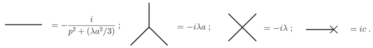
Figure 1: Feynman rules at $\phi_{0}=a$

Let us take a closer look at the case of small tadpoles, that is naturally amenable to a perturbative treatment. This can illustrate a further important subtlety: the diagrams that contribute to this series are not all 1PI, and thus by the usual rules should not all contribute to $\Gamma$. For instance, let us consider the Lagrangian

$${\cal L}\ =\ -\,\frac{1}{2}\,(\partial_{\mu}\phi)^{2}\ -\ \frac{\lambda}{4!}(\phi^{2}-a^{2})^{2}\ +\ c\;\phi\ ,$$ (2.16)

with a Mexican-hat section potential and a driving “magnetic field” represented by the tadpole $c$. The issue is to single out the terms produced in the gaussian expansion of the path integral of eq. (2.16) once the integration variable is shifted about the “wrong” vacuum $\phi_{0}=a$, writing $\phi=a+\chi$, so that

$$e^{\frac{i}{\hbar}\,W[J]}\ =\int[D\phi]\ e^{\frac{i}{\hbar}\int d^{\cal D}x\left(\;-\;\frac{1}{2}\partial_{\mu}\chi\partial^{\mu}\chi\,-\,\frac{\lambda a^{2}}{6}\chi^{2}\,-\,\frac{\lambda a}{3!}\chi^{3}\,-\,\frac{\lambda}{4!}\chi^{4}\,+\,c(a+\chi)\,+\,J(a+\chi)\right)}\ .$$ (2.17)

Notice that, once $\chi$ is rescaled to $\hbar^{1/2}\chi$ in order to remove all powers of $\hbar$ from the gaussian term, in addition to the usual positive powers of $\hbar$ associated to cubic and higher terms, a negative power $\hbar^{-1/2}$ accompanies the tadpole term in the resulting Lagrangian. As a result, the final ${\cal O}(1/\hbar)$ contribution that characterizes the classical vacuum energy results from infinitely many diagrams built with the Feynman rules summarized in fig. 1. The first two non-trivial contributions originate from the three-point vertex terminating on three tadpoles, from the four-point vertex terminating on four tadpoles and from the exchange diagram of fig. 2.

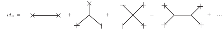
Figure 2: Vacuum energy

As anticipated, tadpoles affect substantially the character of the diagrams contributing to $\Gamma$, and in particular to the vacuum energy, that we shall denote by $\Lambda_{0}$. Beginning from the latter, let us note that, in the presence of a tadpole coupling $c$,

$$e^{-\frac{i}{\hbar}\Lambda_{0}\,{\cal V}}\ =\ \int[D\phi]\ e^{\frac{i}{\hbar}\left(S[\phi]\,+\,\int d^{\cal D}x\;c\phi\right)}\ ,$$ (2.18)

where ${\cal V}$ denotes the volume of space time. Hence, the vacuum energy is actually determined by a power series in $c$ whose coefficients are connected, rather than 1PI, amplitudes, since they are Green functions of W computed for a classical value of the current determined by $c$:

$$-\,\frac{i}{\hbar}\,\Lambda_{0}\,{\cal V}\ =\ \sum_{n}\ \frac{(i\;c)^{n}}{n!\;\hbar^{n}}\ W^{(n)}[\{p_{j}=0\}]\ .$$ (2.19)

A similar argument applies to the higher Green functions of $\Gamma$: the standard Legendre transform becomes effectively in this case

$$W[J+c]\ =\ \Gamma[\bar{\phi}]\ +\ J\bar{\phi}\ ,$$ (2.20)

since the presence of a tadpole shifts the argument of W. However, the l.h.s. of (2.20) contains an infinite series of conventional connected Green functions, and after the Legendre transform only those portions that do not depend on the tadpole $c$ are turned into 1PI amplitudes. The end conclusion is indeed that the contributions to $\Gamma$ that depend on the tadpoles involve arbitrary numbers of connected, but also non 1PI, diagrams.

The vacuum energy is a relatively simple and most important quantity that one can deal with from this viewpoint, and its explicit study will help to clarify the meaning of eq. (2.13). Using eqs. (2.8) and (2.10) one can indeed conclude that, at the classical level,

$$\Lambda_{0}\ =\ -\,\frac{W(J=0)}{\cal V}\ =\ -\,V(\phi_{0})\ -\ \frac{i}{2}\ \Delta\,\left.{\cal D}\right|_{p^{2}=0}\Delta+{\cal O}(\Delta^{3})\ ,$$ (2.21)

an equation that we shall try to illustrate via a number of examples in this paper. The net result of this Subsection is that resummations around a wrong vacuum lead nonetheless to extrema of the effective action. However, it should be clear from the previous derivation that the scalar propagator must be nonsingular, or equivalently the potential must not have an inflection point at $\phi_{0}$, in order that the perturbative corrections about the original wrong vacuum be under control. A related question is whether the resummation flow converges generically towards minima (local or global) or can end up in a maximum. As we shall see in detail shortly, the end point is generally an extremum and not necessarily a local minimum.

2-b. The end point of the resummation flow

The purpose of this Section is to investigate, for some explicit forms of the scalar potential $V(\phi)$ and for arbitrary initial values of the scalar field $\phi_{0}$, the end point reached by the system after classical tadpole resummations are performed. The answer, that will be justified in a number of examples, is as follows: starting from a wrong vacuum $\phi_{0}$, the system typically reaches a nearby extremum (be it a minimum or a maximum) of the potential not separated from it by any inflection. While this is the generic behavior, we shall also run across a notable exception to this simple rule: there exist some peculiar “large” flows, corresponding to special values of $\phi_{0}$, that can actually reach an extremum by going past an inflection, and in fact even crossing a barrier, but are nonetheless captured by the low orders of the perturbative expansion!

An exponential potential is an interesting example that is free of such inflection points, and is also of direct interest for supersymmetry breaking in String Theory. Let us therefore begin by considering a scalar field with the Lagrangian

$${\cal L}\ =\ -\,\frac{1}{2}\,\partial^{\mu}\phi\,\partial_{\mu}\phi\ -\ \alpha\ e^{b\phi}\ ,$$ (2.22)

where for definiteness the two coefficients $\alpha$ and $b$ are both taken to be positive. The actual minimum is reached as $\phi\to-\infty$, where the classical vacuum energy vanishes.

In order to recover this result from a perturbative expansion around a generic “wrong” vacuum $\phi_{0}$, let us shift the field, writing $\phi=\phi_{0}+\chi$. The Feynman rules can then be extracted from

$${\cal L}_{eff}=-\,\frac{1}{2}\ \partial^{\mu}\chi\,\partial_{\mu}\chi\ -\ \frac{\Delta}{b}\ e^{b\chi}\ ,$$ (2.23)

where $\Delta$, the one-point function in the “wrong” vacuum, is defined by

$$-\ \left.\frac{\delta{\cal L}_{eff}}{\delta\phi}\right|_{\phi_{0}}\ =\ \Delta\ =\ \alpha\ b\ e^{b\phi_{0}}\ ,$$ (2.24)

and the first few contributions to the classical vacuum energy are as in fig. 3.

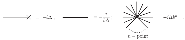
Figure 3: Feynman rules for the exponential potential

It is fairly simple to compute the first few diagrams. For instance, the two-tadpole correction to $-iV(\phi_{0})$ is

$$\ \frac{1}{2}\ \frac{-i}{b\Delta}\ (-i\Delta)^{2}=-\frac{1}{2}\left(\frac{-i\Delta}{b}\right)\ ,$$ (2.25)

while the three-tadpole correction, still determined by a single diagram, is

$$\frac{1}{3!}\ (-i\Delta\ b^{2})\ (-i\Delta)^{3}\left(\frac{-i}{b\Delta}\right)^{3}\ =\ -\ \frac{1}{6}\left(\frac{-i\Delta}{b}\right)\ .$$ (2.26)

On the other hand, the quartic contribution is determined by two distinct diagrams, and equals

$$\frac{1}{4!}\ (-i\Delta\ b^{3})\ (-i\Delta)^{4}\left(\frac{-i}{b\Delta}\right)^{4}+\frac{1}{8}\ (-i\Delta\ b^{2})^{2}\ (-i\Delta)^{4}\left(\frac{-i}{b\Delta}\right)^{5}\ =\ -\ \frac{1}{12}\left(\frac{-i\Delta}{b}\right)\ ,$$ (2.27)

while the quintic contribution originates from three diagrams. Putting it all together, one obtains

$$\Lambda_{0}\ =\ \frac{\Delta}{b}\ \left(1-\frac{1}{2}-\frac{1}{6}-\frac{1}{12}-\frac{1}{20}+\ldots\right)\ =\ \frac{\Delta}{b}\left[1-\sum_{n=1}^{\infty}\frac{1}{n(n+1)}\right]\ .$$ (2.28)

The resulting pattern is clearly identifiable, and suggests in an obvious fashion the series in (2.28). Notice that, despite the absence of a small expansion parameter, in this example the series in (2.28) actually converges to $1$, so that the correct vanishing value for the classical vacuum energy can be exactly recovered from an arbitrary wrong vacuum $\phi_{0}$.

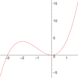
Figure 4: A cubic potential

We can now turn to a more intricate example and consider the model (fig. 4)

$${\cal L}\ =\ -\,\frac{1}{2}(\partial_{\mu}\phi)^{2}\ -\ \frac{m^{2}\phi^{2}}{2}\ -\ \frac{\lambda\phi^{3}}{6}\ ,$$ (2.29)

the simplest setting where one can investigate the role of an inflection. Strictly speaking this example is pathological, since its Hamiltonian is unbounded from below, but for our purpose of gaining some intuition on classical resummations it is nonetheless instructive. The two extrema of the scalar potential $v_{1,2}$ and the inflection point $v_{I}$ are

$$v_{1}=0\ ,\quad v_{2}=-\frac{2m^{2}}{\lambda}\ ,\quad v_{I}=-\frac{m^{2}}{\lambda}\ .$$ (2.30)

Starting from an arbitrary initial value $\phi_{0}$, let us investigate the convergence of the resummation series and the resulting resummed value $\langle\phi\rangle$. A close look at the diagrammatic expansion indicates that

$$\langle\phi\rangle\ =\ \phi_{0}+\ \frac{V^{\prime}}{V^{{}^{\prime\prime}}}\ \sum_{n=0}^{\infty}c_{n}\left[\frac{\lambda V^{\prime}}{(V^{{}^{\prime\prime}})^{2}}\right]^{n}\ \equiv\ \phi_{0}+\frac{V^{\prime}}{V^{{}^{\prime\prime}}}\ f(x)\ ,$$ (2.31)

where the actual expansion variable is

$$x\ =\ \frac{\lambda V^{\prime}}{(V^{{}^{\prime\prime}})^{2}}\ ,$$ (2.32)

to be contrasted with the naive dimensionless expansion variable

$$z=\frac{\lambda\phi_{0}}{m^{2}}\ .$$ (2.33)

According to eq. (2.32), their relation is

$$x=\frac{z(z+2)}{2(z+1)^{2}}\ ,$$ (2.34)

whose inverse is

$$z=-1\ \mp\ \frac{1}{\sqrt{1-2x}}\ ,$$ (2.35)

where the upper sign corresponds to the region $(L)$ to the left of the inflection, while the lower sign corresponds to the region $(R)$ to the right of the inflection. In other words: $\phi_{0}$, and thus the naive variable $z$ of the problem, is actually a double-valued function of $x$, while the actual range covered by $x$ terminates at the inflection.

A careful evaluation of the symmetry factors of various diagrams with variable numbers of tadpole insertions shows that

$$f(x)\ =\ -\,\frac{\sqrt{\pi}}{2}\sum_{n=0}^{\infty}\frac{(-1)^{n}\ 2^{n+1}}{(n+1)!\ \Gamma{(1/2-n)}}\ x^{n}\ ,$$ (2.36)

a series that for $|x|<1/2$ converges to

$$f(x)\ =\ -\,\frac{1}{x}\ +\ \frac{\sqrt{1-2x}}{x}\ .$$ (2.37)

The relation between $z$ and $x$ implies that both $\phi_{0}$ and $V^{{}^{\prime\prime}}$ have two different expressions in terms of $x$ on the two sides of the inflection,

$$V^{{}^{\prime\prime}}=\pm\frac{m^{2}}{\sqrt{1-2x}}\quad,\quad\phi_{0}=-\frac{m^{2}}{\lambda}\mp\frac{m^{2}}{\lambda}\frac{1}{\sqrt{1-2x}}\ ,$$ (2.38)

where the upper signs apply to the region $(L)$ that lies to the left of the inflection, while the lower signs apply to the region $(R)$ that lies to the right of the inflection. Combining (2.37) and (2.38) finally yields the announced result:

$$\langle\phi\rangle\rightarrow 0\quad{\rm in\ the\ (R)\ region:}\quad-\frac{m^{2}}{\lambda}<\phi_{0}<\infty\ ,$$

$$\langle\phi\rangle\rightarrow-\frac{2m^{2}}{\lambda}\quad{\rm for\ in\ (L)\ region:}\quad-\infty<\phi_{0}<-\frac{m^{2}}{\lambda}\ .$$ (2.39)

The resummation clearly breaks down near the inflection point $v_{I}$. In the present case, the series in (2.37) converges for $|x|<1/2$, and this translates into the condition

$$\phi_{0}\in\left(-\infty,-\frac{m^{2}}{\lambda}\left(1+\frac{1}{\sqrt{2}}\right)\right)\ \bigcup\ \left(-\frac{m^{2}}{\lambda}\left(1-\frac{1}{\sqrt{2}}\right),\infty\right)\ .$$ (2.40)

A symmetric interval around the inflection point thus lies outside this region, while in the asymptotic regions $\phi_{0}\rightarrow\pm\infty$ the parameter $x$ tends to $1/2$, a limiting value for the convergence of the series (2.36).

The vacuum energy $\Lambda_{0}$ is another key quantity for this problem. Starting as before from an arbitrary initial value $\phi_{0}$, standard diagrammatic methods indicate that

$$\Lambda_{0}=\ V(\phi_{0})+\ \frac{(V^{\prime})^{2}}{V^{{}^{\prime\prime}}}\ \sum_{n=0}^{\infty}d_{n}\left[\frac{\lambda V^{\prime}}{(V^{{}^{\prime\prime}})^{2}}\right]^{n}\ \equiv\ V(\phi_{0})+\frac{(V^{\prime})^{2}}{V^{{}^{\prime\prime}}}\ h(x)\ .$$ (2.41)

A careful evaluation of the symmetry factors of various diagrams with arbitrary numbers of tadpole insertions then shows that

$$h(x)\ =\ -\,\frac{\sqrt{\pi}}{4}\sum_{n=0}^{\infty}\frac{(-1)^{n}\ 2^{n+2}}{(n+2)!\ \Gamma{(1/2-n)}}\ x^{n}\ ,$$ (2.42)

that for $|x|<1/2$ converges to

$$h(x)\ =\ \frac{1}{3x^{2}}\left[1-3x-(1-2x)^{3/2}\right]\ .$$ (2.43)

The two different relations between $z$ and $x$ in (2.35) that apply to the two regions $(L)$ and $(R)$ finally yield:

$$\Lambda_{0}\rightarrow 0\ ,\quad{\rm in\ the\ (R)\ region}\ -\frac{m^{2}}{\lambda}<\phi_{0}<\infty\ ,$$

$$\Lambda_{0}\rightarrow\frac{2m^{6}}{3\lambda^{2}}\ ,\quad{\rm in\ the\ (L)\ region}\ -\infty<\phi_{0}<-\frac{m^{2}}{\lambda}\ .$$ (2.44)

To reiterate, we have seen how in this model the resummations approach nearby extrema (local minima or maxima) not separated from the initial value $\phi_{0}$ by any inflection.

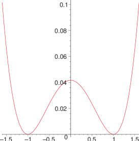
Figure 5: A quartic potential

A physically more interesting example is provided by a real scalar field described by the Lagrangian (fig. 5)

$${\cal L}\ =\ -\,\frac{1}{2}(\partial_{\mu}\phi)^{2}\ -\ \frac{\lambda}{4!}\;(\phi^{2}-a^{2})^{2}\ ,$$ (2.45)

whose potential has three extrema, two of which are a pair of degenerate minima, $v_{1}=-a$ and $v_{3}=+a$, separated by a potential wall, while the third is a local maximum at the origin. Two inflection points are now present,

$$v^{(1)}_{I}=-\frac{a}{\sqrt{3}}\ ,\qquad v^{(2)}_{I}=\frac{a}{\sqrt{3}}\ ,$$ (2.46)

that also form a symmetric pair with respect to the vertical axis.

Starting from an arbitrary initial value $\phi_{0}$, one can again in principle sum all the diagrams, and a closer look shows that there are a pair of natural variables, $y_{1}$ and $y_{2}$, defined as

$$y_{1}\ =\ \phi_{0}\ \frac{\lambda V^{\prime}}{(V^{{}^{\prime\prime}})^{2}}\qquad{\rm and}\qquad y_{2}\ =\ \frac{\lambda{V^{\prime}}^{2}}{(V^{{}^{\prime\prime}})^{3}}\ ,$$ (2.47)

that reflect the presence of the cubic and quartic vertices and depend on the square of $\phi_{0}$. On the other hand, the naive dimensionless variable to discuss the resummation flow is in this case

$$z=\phi_{0}^{2}/{a}^{2}\ ,$$ (2.48)

and eqs. (2.47) imply that

$$y_{1} = 6\,\frac{z(z-1)}{(3z-1)^{2}}\ ,$$ (2.49)

$$y_{2} = 6\,\frac{z(z-1)^{2}}{(3z-1)^{3}}\ .$$ (2.50)

The diagrammatic expansions of $\langle\phi\rangle$ and $\Lambda_{0}$ are now more complicated than in the $\phi^{3}$ example. A careful evaluation of the symmetry factors of various diagrams, however, uncovers an interesting pattern, since

$$\langle\phi\rangle = \phi_{0}+\frac{V^{\prime}}{V^{{}^{\prime\prime}}}\left[-1-\frac{1}{2}\left(y_{1}-\frac{y_{2}}{3}\right)-\frac{1}{2}\left(y_{1}-\frac{y_{2}}{3}\right)\left(y_{1}-\frac{y_{2}}{2}\right)\right.$$

$$- \left.\frac{5}{8}\left(y_{1}-\frac{y_{2}}{3}\right)\left(y_{1}-\frac{2y_{2}}{3}\right)\left(y_{1}-\frac{2y_{2}}{5}\right)\right.$$

$$- \left.\frac{7}{8}\left(y_{1}-\frac{y_{2}}{3}\right)\left(y_{1}^{3}-\frac{5}{3}y_{1}^{2}y_{2}+\frac{55}{63}y_{1}y_{2}^{2}-\frac{55}{378}y_{2}^{3}\right)\right.$$

$$- \frac{21}{16}\ \left.\left(y_{1}-\frac{y_{2}}{3}\right)\left(y_{1}^{4}-\frac{16}{7}y_{1}^{3}y_{2}+\frac{13}{7}y_{1}^{2}y_{2}^{2}-\frac{52}{81}y_{1}y_{2}^{3}+\frac{13}{162}y_{2}^{4}\right)+\cdots\right]\ ,$$

$$\Lambda_{0} = V(\phi_{0})+\frac{(V^{\prime})^{2}}{V^{{}^{\prime\prime}}}\left[-\frac{1}{2}-\frac{1}{6}\left(y_{1}-\frac{y_{2}}{4}\right)-\frac{1}{8}\left(y_{1}-\frac{y_{2}}{3}\right)^{2}-\frac{1}{8}\left(y_{1}-\frac{y_{2}}{3}\right)^{2}\left(y_{1}-\frac{1}{2}y_{2}\right)\right.$$ (2.51)

$$- \frac{7}{48}\left.\left(y_{1}-\frac{y_{2}}{3}\right)^{2}\,\left(y_{1}^{2}-\frac{22}{21}y_{1}y_{2}+\frac{11}{42}y_{2}^{2}\right)\right.$$

$$- \left.\frac{3}{16}\left(y_{1}-\frac{y_{2}}{3}\right)^{2}\left(y_{1}^{3}-\frac{13}{8}y_{1}^{2}y_{2}+\frac{91}{108}y_{1}y_{2}^{2}-\frac{91}{648}y_{2}^{3}\right)+\cdots\right]\ ,$$

where all linear and higher-order corrections in $\langle\phi\rangle$ and all quadratic and higher order corrections in $\Lambda_{0}$ apparently disappear at the special point $y_{1}=y_{2}/3$. Notice that this condition identifies the three extrema $\phi_{0}=\pm a$ and $\phi_{0}=0$, but also, rather surprisingly, the two additional points $\phi_{0}=\pm\frac{a}{2}$. In all these cases the series expansions for $\langle\phi\rangle$ and $\Lambda_{0}$ apparently end after a few terms.

If one starts from a wrong vacuum sufficiently close to one of the extrema, one can convince oneself that, in analogy with the previous example ,

$$\langle\phi\rangle\rightarrow-a\quad,\quad{\rm for\ region\ 1:}\quad-\infty<\phi_{0}<v^{(1)}_{I}\ ,$$

$$\langle\phi\rangle\rightarrow 0\quad,\quad{\rm for\ region\ 2:}\quad v^{(1)}_{I}<\phi_{0}<v^{(2)}_{I}\ ,$$

$$\langle\phi\rangle\rightarrow+a\quad,\quad{\rm for\ region\ 3:}\quad v^{(2)}_{I}<\phi_{0}<\infty\ ,$$ (2.52)

but we have not arrived at a single natural expansion parameter for this problem, an analog of the variable $x$ of the cubic potential. In addition, while these perturbative flows follow the pattern of the previous example, since they are separated by inflections that act like barriers, a puzzling and amusing result concerns the special initial points

$$\phi_{0}=\pm\frac{a}{2}\ .$$ (2.53)

In this case $y_{2}=3y_{1}$ and, as we have seen, apparently all but the first few terms in $\langle\phi\rangle$ and all but the first few terms in $\Lambda_{0}$ vanish. The non-vanishing terms in eq. (2.51) show explicitly that the endpoints of these resummation flows correspond to $\langle\phi\rangle=\pm a$ for $\phi_{0}=\mp\frac{a}{2}$, and that $\Lambda_{0}=0$, so that these two flows apparently “cross” the potential barrier and pass beyond an inflection. One might be tempted to dismiss this phenomenon, since after all this is a case with large tadpoles (and large values of $y_{1}$ and $y_{2}$), that is reasonably outside the region of validity of perturbation theory and hence of the strict range of applicability of eq. (2.51). Still, toward the end of this Subsection we shall encounter a similar phenomenon, clearly within a perturbative setting, where the resummation will unquestionably collapse to a few terms to land at an extremum, and therefore it is worthwhile to pause and devote to this issue some further thought.

Interestingly, the tadpole resummations that we are discussing have a simple interpretation in terms of Newton’s method of tangents, a very effective iterative procedure to derive the roots of non-linear algebraic equations. It can be simply adapted to our case, considering the function $V^{\prime}(\phi)$, whose zeroes are the extrema of the scalar potential. The method begins with guess, a “wrong vacuum” $\phi_{0}$, and proceeds via a sequence of iterations determined by the zeros of the sequence of straight lines

$$y-V^{\prime}(\phi^{(n)})\ =\ V^{{}^{\prime\prime}}(\phi^{(n)})\ (x-\phi^{(n)})\ ,$$ (2.54)

that are tangent to the curve at subsequent points, defined recursively as

$$\phi^{(n+1)}\ =\ \phi^{(n)}\ -\ \frac{V^{\prime}(\phi^{(n)})}{V^{{}^{\prime\prime}}(\phi^{(n)})}\ ,$$ (2.55)

where $\phi^{(n)}$ denotes the $n$-th iteration of the wrong vacuum $\phi^{(0)}=\phi_{0}$.

When applied to our case, restricting our attention to the first terms the method gives

$$\phi^{(1)} = \phi_{0}-\frac{V^{\prime}}{V^{{}^{\prime\prime}}}\ ,$$

$$\phi^{(2)} = \phi^{(1)}-\frac{V^{\prime}(\phi^{(1)})}{V^{{}^{\prime\prime}}(\phi^{(1)})}=\phi_{0}+\frac{V^{\prime}}{V^{{}^{\prime\prime}}}\left[\,-1\ -\ \frac{\frac{V^{\prime}\;V^{{}^{\prime\prime\prime}}}{2(V^{{}^{\prime\prime}})^{2}}-\frac{(V^{\prime})^{2}\;V^{{}^{\prime\prime\prime\prime}}}{6(V^{{}^{\prime\prime}})^{3}}}{1-\frac{V^{\prime}V^{{}^{\prime\prime\prime}}}{(V^{{}^{\prime\prime}})^{2}}+\frac{(V^{\prime})^{2}V^{{}^{\prime\prime\prime\prime}}}{2(V^{{}^{\prime\prime}})^{3}}}\,\right]$$ (2.56)

$$\cong \phi_{0}+\frac{V^{\prime}}{V^{{}^{\prime\prime}}}\biggl{[}-1-\frac{1}{2}(y_{1}-\frac{y_{2}}{3})-\frac{1}{2}(y_{1}-\frac{y_{2}}{3})(y_{1}-\frac{y_{2}}{2})\biggr{]}\ ,$$

where $y_{1}$ and $y_{2}$ are defined in (2.47) and, for brevity, the arguments are omitted whenever they are equal to $\phi_{0}$. Notice the precise agreement with the first four terms in (2.51), that imply that our tadpole resummations have a simple interpretation in terms of successive iterations of the solutions of the vacuum equations $V^{\prime}=0$ by Newton’s method. Notice the emergence of the combination $y_{1}-y_{2}/3$ after the first iteration: as a result, the pattern of eqs. (2.51) continues indeed to all orders.

In view of this interpretation, the non-renormalization points $\phi_{0}=\pm a/2$ acquire a clear geometrical interpretation: in these cases the iteration stops after the first term $\phi^{(1)}$, since the tangent drawn at the original “wrong” vacuum, say at $a/2$, happens to cross the real axis precisely at the extremum on the other side of the barrier, at $\langle\phi\rangle=-a$. Newton’s method can also shed some light on the behavior of the iterations, that stay on one side of the extremum or pass to the other side according to the concavity of the potential, and on the convergence radius of our tadpole resummations, that the second iteration already restricts $y_{1}$ and $y_{2}$ to the region

$$\left|y_{1}\ -\ \frac{y_{2}}{2}\right|\ <\ 1\ .$$ (2.57)

However, the tangent method behaves as a sort of Dyson resummation of the naive diagrammatic expansion, and has therefore better convergence properties. For instance, starting near the non-renormalization point $\phi_{0}\simeq-a/2$, the first iteration lands far away, but close to the minimum $\phi^{(1)}\simeq a$. The second correction, that when regarded as a resummation in (2.51) is large, is actually small in the tangent method, since it is proportional to $(1/16)(y_{1}-y_{2}/3)$. It should be also clear by now that not only the points $\phi_{0}=\pm a/2$, but finite intervals around them, move across the barrier as a result of the iteration. These steps, however, do not have a direct interpretation in terms of Feynman diagram tadpole resummations, since (2.57) is violated, so that the corresponding diagrammatic expansion actually diverges. The reason behind the relative simplicity of the cubic potential (2.29) is easily recognized from the point of view of the tangent method: the corresponding $V^{\prime}(\phi)$ is a parabola, for which Newton’s method never leads to tangents crossing the real axis past an inflection point.

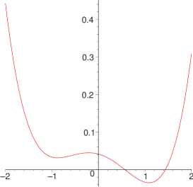
Figure 6: A quartic potential with a “magnetic” deformation

There is a slight technical advantage in returning to the example of eq. (2.16), since for a small magnetic field (tadpole) $c$ (fig. 6) one can expand the complete expressions for the vacuum energy and the scalar v.e.v.’s in powers of the tadpole. The expansions (2.51) still apply, with an obvious change in the one-point function $V^{\prime}$, and their sums should coincide, term by term, with the tadpole resummations obtained starting from the undeformed “wrong” vacua $\phi_{0}=\pm a,0$.

In this case the vacuum energy is given by

$$\Lambda_{0}\ =\ \frac{\lambda}{4!}\,(v^{2}-a^{2})^{2}\ -\ c\;v\ ,$$ (2.58)

where the correct vacuum value $\langle\phi\rangle=v$ is determined by the cubic equation

$$\lambda\frac{v}{6}\;(v^{2}-a^{2})\ -\ c\ =\ 0\ ,$$ (2.59)

that can be easily solved perturbatively in the tadpole $c$, so that if one starts around $\phi_{0}=a$,

$$\Lambda_{0}\ =\ -\,c\;a\ -\ \frac{3c^{2}}{2\lambda a^{2}}\ +\ {\cal O}(c^{3})\ .$$ (2.60)

This result can be also recovered rather simply starting from the wrong vacuum $\phi_{0}=a$ and making use of eq. (2.21), since in this case $\Delta=-c$ and ${\cal D}(p^{2}=0)=-3i/\lambda a^{2}$. However, the cubic equation (2.59) can be also solved exactly in terms of radicals, and in the small tadpole limit its three solutions are real and can be written in the form

$$v\ =\ \frac{2a}{\sqrt{3}}\ \cos\left[\frac{\alpha}{3}+\frac{2\pi k}{3}\right]\qquad(k=0,1,2)\ ,$$ (2.61)

where

$$\cos(\alpha)=\xi\ ,\qquad\sin(\alpha)=\sqrt{1-\xi^{2}}\ ,\quad{\rm with}\quad\xi=\frac{9\sqrt{3}c}{\lambda a^{3}}\ .$$ (2.62)

For definiteness, let us consider a tadpole $c$ that is small and positive, so that the absolute minimum of the deformed potential lies in the vicinity of the original minimum of the Mexican-hat section at $v=a$ and corresponds to $k=0$. We can now describe the fate of the resummations that start from two different wrong vacua:

i) $\phi_{0}=a$. In this case and in the small tadpole limit $\xi<<1$ resummations in the diagrammatic language produce the first corrections

$$\langle\phi\rangle=a+\frac{3c}{\lambda a^{2}}-\frac{27c^{2}}{2\lambda^{2}a^{5}}+\cdots\ .$$ (2.63)

Alternatively, this result could be obtained solving eq. (2.59) in powers of the tadpole $c$ with the initial value $\phi_{0}=a$, so that, once more, starting from a wrong vacuum close to an extremum and resumming one can recover the correct answer order by order in the expansion parameter. In this case both a cubic and a quartic vertex are present, and the complete expression for the vacuum energy, obtained substituting (2.61) in (2.58), is

$$\Lambda_{0}\ =\ \frac{2\;\lambda a^{4}\;\xi}{27}\ \left[\frac{\xi}{16}\,\frac{1}{\cos^{2}\left(\frac{\alpha}{3}\right)}\ -\ \cos\left(\frac{\alpha}{3}\right)\right]\ .$$ (2.64)

This can be readily expanded in a power series in $\xi$, whose first few terms,

$$\Lambda_{0}\ =\ -a\;c\ -\ \frac{\sqrt{3}}{18}\;a\;c\;\xi\ +\ \frac{1}{54}\;a\;c\;\xi^{2}\ -\ \frac{\sqrt{3}}{243}\;a\;c\;\xi^{3}\ +\ {\cal O}(\xi^{4})\ .$$ (2.65)

match precisely the tadpole expansion (2.51).

ii) $\phi_{0}=0$. In this case the first corrections obtained resumming tadpole diagrams are

$$\langle\phi\rangle=-\frac{6c}{\lambda a^{2}}-\frac{216c^{3}}{\lambda^{3}a^{8}}+\cdots\ .$$ (2.66)

The same result can be obtained expanding the solution of (2.59) in powers of the tadpole $c$, starting from the initial value $\phi_{0}=0$. We can now compare (2.61) with (2.51), noting that in this case only the quartic vertex is present, so that $y_{1}=0$. Since $y_{2}=-8\xi^{2}/9$ for $\phi_{0}=0$, the v.e.v. $\langle\phi\rangle$ contains only odd powers of the tadpole $c$, a property that clearly holds in (2.61) as well, since $\xi\rightarrow-\xi$ corresponds to $\alpha\rightarrow\alpha+(2l+1)3\pi$, with $l$ integer and $v\rightarrow-v$ in (2.61). The contributions to $\langle\phi\rangle$ are small and negative, and therefore, starting from a wrong vacuum close to a maximum of the theory, the resummation flow leads once more to a nearby extremum (the local maximum slightly to the left of the origin, in this case), rather than rolling down to the minimum corresponding to the $k=0$ solution of (2.61). The important points in the scalar potential are again the extrema and the inflections, precisely as we had seen in the example with a cubic potential. Barring the peculiar behavior near the points identified by the condition $y_{1}=y_{2}/3$, the scalar field flows in general to the nearest extremum (minimum or maximum) of this potential, without passing through any inflection point along the whole resummation flow. It should be appreciated how the link with Newton’s method associates a neat geometrical interpretation to this behavior.

For $\xi=1$ the two extrema of the unperturbed potential located at $\ v=-a\$ and at $\ v=0\$ coalesce with the inflection at $-a/\sqrt{3}$. If the potential is deformed further, increasing the value of the tadpole, the left minimum disappears and one is left with only one real solution, corresponding to $k=0$. The correct parameterization for $\ \xi>1\$ is $\ \cosh(\alpha)=\xi\$ and $\ \sinh(\alpha)=\sqrt{\xi^{2}-1}\$, and the classical vacuum energy is like in (2.64), but with $\ \cos(\alpha/3)$ replaced by $\cosh(\alpha/3)$. In order to recover the result (2.65) working perturbatively in the “wrong” vacuum $v=a$, one should add the contributions of an infinite series of diagrams that build a power series in $1/\xi$, but this cannot be regarded as a tadpole resummation anymore. The meaning of the parameter $\xi$ should by now have become apparent: it is proportional to the product of the tadpole and the propagator in the wrong vacuum, $V^{\prime}/V^{\prime\prime}$, a natural expansion parameter for problems of this type. Notice that the ratio $V^{\prime}/V^{{}^{\prime\prime}}$ is twice as large (and of opposite sign) at the origin $\phi_{0}=0$ than at $\phi_{0}=a$. Therefore, the tadpole expansion first breaks down around $\phi_{0}=0$. As we have seen, the endpoint of the resummation flow for $\phi_{0}=0$ is the local maximum corresponding to $k=2$ in (2.61), that is reached for $\xi<1$. At $\xi=1$, however, the two extrema corresponding to $k=1$ and $k=2$ coalesce with the inflection at $-a/\sqrt{3}$, and hence there is no possible endpoint for the resummation flow. This is transparent in (2.61), since for $\xi\geq 1$ the $\xi$ expansion clearly breaks down. It should therefore be clear why, if the potential is deformed too extensively, corresponding to $\ \xi>1$, a perturbative expansion around the extrema $\ v=\pm a,0\$ in powers of $\xi$ is no longer possible. Another key issue that should have emerged from this discussion is the need for an independent, small expansion parameter when tadpoles are to be treated perturbatively. In this example, as anticipated, the expansion parameter $\xi$ can be simply related to the potential according to

$$\xi\ =\ \frac{3\sqrt{3}}{a}\ \left|\frac{V^{\prime}}{V^{\prime\prime}}\right|\ ,$$ (2.67)

that is indeed small if $c$ is small.

It is natural to ask about the fate of the points $\phi_{0}=\pm a/2$ of the previous example (2.45) when the magnetic field $c$ is turned on. Using the parameters $y_{i}$ in (2.47), the condition determining these special points, $y_{1}=y_{2}/3$, is equivalent to

$$V^{\prime}\ =\ 3\ \phi_{0}\ V^{{}^{\prime\prime}}\ .$$ (2.68)

It is readily seen that the solutions of this cubic equation are precisely $\phi_{0}=-v/2$, if $v$ denotes, collectively, the three extrema solving (2.59). Hence, in this case $\langle\phi\rangle=-2\phi_{0}=v$, confirming the persistence of these non-renormalization points. In the present case, however, there is a third non-renormalization point, $\phi_{0}=-v_{k=2}/2$, that for small values of $\xi$ is well inside the convergence region. This last point clearly admits an interpretation in terms of tadpole resummations, and the possible existence of effects of this type in String Theory raises the hope that explicit vacuum redefinitions could be constructed in a few steps for special values of the string coupling and of other moduli.

2-c. Branes and tadpoles of codimension one

Models whose tadpoles are confined to lower-dimensional surfaces are of particular interest. In String Theory there are large classes of examples of this type, including brane supersymmetry breaking models [4, 5], intersecting brane models [7] and models with internal fluxes [13]. If the space transverse to the branes is large, the tadpoles are ”diluted” and there is a concrete hope that their corrections to brane observables be small, as anticipated in [5]. In the codimension one case, tadpoles reflect themselves in boundary conditions on the scalar (dilaton) field and hence on its propagator, and as a result their effects on the Kaluza-Klein spectrum and on brane-bulk couplings are nicely tractable.

Let us proceed by considering again simple toy models that display the basic features of lower-dimensional tadpoles. The internal spacetime is taken to be $S^{1}/Z_{2}$, with $S^{1}$ a circle, and the coordinate of the circle is denoted by $y$: in a string realization its two endpoints $y=0$ and $y=\pi R$ would be the two fixed points of the orientifold operation $\Omega^{\prime}=\Omega\ \Pi_{y}$, with $\Pi_{y}$ the parity in $y$. We also let the scalar field interact with a boundary gauge field, so that

$$S=\int d^{4}{\bf x}\int_{0}^{\pi R}dy\biggl{\{}\ -\frac{1}{2}({\partial\phi})^{2}\ -\ \left(T\ \phi\ +\ \frac{m}{2}\ \phi^{2}\ -\ \phi\ {\rm tr\,}(F^{2})\right)\ \delta(y-\pi R)\ \biggr{\}}\ .$$ (2.69)

The Lagrangian of this toy model describes a free massless scalar field living in the bulk, but with a tadpole and a mass-like term localized at one end of the interval $[0,\pi R]$. In String Theory, both the mass-like parameter $m$ and the tadpole $T$ in the examples we shall discuss would be perturbative in the string coupling constant $g_{s}$. Any non-analytic IR behavior associated with the possible emergence of $1/m$ terms would thus signal a breakdown of perturbation theory, according to the discussion presented in the Introduction. Notice that, for dimensional reasons, the mass term is proportional to $m$, rather than to $m^{2}$ as is usually the case for bulk masses.

The starting point is the Kaluza-Klein expansion

$$\phi({\bf x},y)\ =\ \phi_{c}(y)+\sum_{k}\chi_{k}(y)\ \phi_{k}({\bf x})\ ,$$ (2.70)

where $\phi_{c}(y)$ is the classical field and the $\phi_{k}({\bf x})$ are higher Kaluza-Klein modes. The classical field $\ \phi_{c}\ =\ -\ T/m\$ solves the simple differential equation

$$\phi_{c}^{{}^{\prime\prime}}\ =\ 0\$$ (2.71)

in the internal space, with the boundary conditions

$$\phi_{c}^{{}^{\prime}}\ =\ 0\ \qquad{\rm at}\ y=0\ ,$$

$$\phi_{c}^{{}^{\prime}}\ =\ -\ T\ -\ m\ \phi_{c}\ \qquad{\rm at}\ y=\pi R\ ,$$ (2.72)

while the Kaluza-Klein modes satisfy in the internal space the equations

$$\chi_{k}^{{}^{\prime\prime}}\ +\ M_{k}^{2}\ \chi_{k}\ =\ 0\ ,$$ (2.73)

with the boundary conditions

$$\chi_{k}^{{}^{\prime}}\ =\ 0\quad{\rm at}\quad y\ =\ 0\ ,$$

$$\chi_{k}^{{}^{\prime}}\ =\ -\ m\ \chi_{k}\quad{\rm at}\quad{\rm at}\ y\ =\ \pi R\ .$$ (2.74)

The corresponding solutions are then

$$\chi_{k}(y)\ =\ A_{k}\ \cos{(M_{k}y)}\ ,$$ (2.75)

where the masses $M_{k}$ of the Kaluza-Klein modes are determined by the eigenvalue equation

$$M_{k}\tan{(M_{k}\pi R)}\ =\ m\ .$$ (2.76)

The classical vacuum energy can be computed directly working in the “right” vacuum. To this end, one ignores the Kaluza-Klein fluctuations and evaluates the classical action in the correct vacuum, as determined by the zero mode, with the end result that

$$\Lambda_{0}\ =\ -\ \frac{T^{2}}{2m}\ .$$ (2.77)

One can similarly compute in the “right” vacuum the gauge coupling, obtaining

$$\frac{1}{g^{2}}\ =\ -\ \phi_{c}(y=\pi R)\ =\ \frac{T}{m}\ .$$ (2.78)

It is amusing and instructive to recover these results expanding $\phi$ around the “wrong” vacuum corresponding to vanishing values for both $T$ and $m$. The Kaluza-Klein expansion is determined in this case by the Fourier decomposition

$$\phi({\bf x},y)=\frac{1}{\sqrt{\pi R}}\ \sum_{k=0}^{\infty}b_{k}\cos\left(\frac{ky}{R}\right)\ \phi^{(k)}({\bf x})\ ,\$$ (2.79)

where $b_{0}=1$ and $b_{k}=\sqrt{2}$ for $k\neq 0$, that turns the action into

$$S_{KK}\ =\ \int d^{4}{\bf x}\left\{\,-\,\frac{1}{2}\sum_{k,l\geq 0}\phi_{k}\;\mathcal{M}^{2}_{k,l}\;\phi_{l}\ -\ T\sum_{k\geq 0}\frac{b_{k}(-)^{k}}{\sqrt{\pi R}}\,\phi_{k}\right\}\ .$$ (2.80)

Here we are ignoring the kinetic term, since the vacuum energy is determined by the zero momentum propagator, while the mass matrix is

$${\mathcal{M}}^{2}_{kl}\ =\ \frac{k^{2}}{R^{2}}\ \delta_{k,l}\ +\ \frac{m}{\pi R}\ b_{k}b_{l}\ (-)^{k+l}\ .$$ (2.81)

The eigenvalues of this infinite dimensional matrix can be computed explicitly using the techniques in [15]. It is actually a nice exercise to show that the characteristic equation defining the eigenvalues of (2.81) is precisely (2.76), and consequently that the eigenvectors of (2.81) are the fields $\chi_{k}$ defined in (2.75). In fact, multiplying (2.81) by normalized eigenfunctions $\Psi^{\lambda}_{k}$ gives

$$\Psi^{\lambda}_{k}\ =\ (-)^{k}\ \frac{mb_{k}}{\pi R}\ \frac{\sum_{l}b_{l}(-)^{l}\Psi^{\lambda}_{l}}{\lambda^{2}-\frac{k^{2}}{R^{2}}}\ ,$$ (2.82)

so that

$$\langle k|\lambda\rangle\ =\ \Psi_{k}^{\lambda}\ =\ \mathcal{N}_{\lambda}\frac{b_{k}(-)^{k}}{\frac{k^{2}}{R^{2}}-\lambda^{2}}\ .$$ (2.83)

and therefore

$$\sum_{k=0}^{\infty}\frac{b_{k}^{2}}{\lambda^{2}-\frac{k^{2}}{R^{2}}}\ =\ \frac{\pi R}{m}\ .$$ (2.84)

The sum can be related to a well-known representation of trigonometric functions [16],

$${\rm cotg}(\lambda\pi R)\ =\ \frac{\lambda}{\pi R}\ \sum_{k=0}^{\infty}\frac{b_{k}^{2}}{\lambda^{2}-\frac{k^{2}}{R^{2}}}\ ,$$ (2.85)

and hence the eigenvalues of (2.81) coincide with those of (2.76). In order to compute the vacuum energy, one needs in addition the k-component of the eigenvector $|\lambda\rangle$, that can be read from (2.82). The normalization constant $\mathcal{N}_{\lambda}$ in (2.83) is then determined by the condition

$$1\ =\ \langle\lambda|\lambda\rangle\ =\ \mathcal{N}_{\lambda}^{2}\ \sum_{k=0}\frac{b_{k}^{2}}{\left(\frac{k^{2}}{R^{2}}-\lambda^{2}\right)^{2}}\ =\ \frac{\mathcal{N}_{\lambda}^{2}}{2\lambda}\ \frac{d}{d\lambda}\ \sum_{k=0}\frac{b_{k}^{2}}{\frac{k^{2}}{R^{2}}-\lambda^{2}}\ ,$$ (2.86)

that using again eq. (2.76) can be put in the form

$$\mathcal{N}^{2}_{\lambda}\ =\ \frac{2m^{2}\lambda^{2}}{\pi^{2}R^{2}}\ \frac{1}{\lambda^{2}+\alpha^{2}}\ ,$$ (2.87)

with

$$\alpha^{2}=\frac{m}{\pi R}\left(1+\pi R\;m\right)\ .$$ (2.88)

Notice that in the limit $R\,m<<1$, that in a string context, where $m$ would be proportional to the string coupling, would correspond to the small coupling limit [17], the physical masses in (2.76) are approximately determined by the solutions of the linearized eigenvalue equation, so that

$$M_{0}^{2} \cong \frac{m}{\pi R}\ ,$$

$$M_{k}^{2} \cong \frac{k^{2}}{R^{2}}+2\frac{m}{\pi R}\ .$$ (2.89)

One can now recover the classical vacuum energy using eq. (2.21),

$$\Lambda_{0}\ =\ -\frac{i}{2}\,\sum_{k,l}\Delta^{(k)}(y_{1}=\pi R)\,\langle k|{\cal D}({\bf 0}~{};y_{1}=\pi R,y_{2}=\pi R)|l\rangle\,\Delta^{(l)}l(y_{2}=\pi R)\ ,$$ (2.90)

that after inserting complete sets of eigenstates becomes

$$\Lambda_{0}\ =\ -\,\frac{T^{2}}{2\pi R}\sum_{\lambda,k,l}\ b_{k}b_{l}(-)^{k+l}\ \langle k|\Psi_{\lambda}\rangle\ \frac{1}{\lambda^{2}}\ \langle\Psi_{\lambda}|l\rangle\ =\ -\frac{T^{2}}{2\pi R}\sum_{\lambda}\ \frac{\mathcal{N}_{\lambda}^{2}}{\lambda^{2}}\ \left(\sum_{k=0}\frac{b_{k}^{2}}{\frac{k^{2}}{R^{2}}-\lambda^{2}}\right)^{2}\ ,$$ (2.91)

or, equivalently, using eq. (2.84)

$$\Lambda_{0}\ =\ -\,\frac{T^{2}}{\pi R}\ \sum_{\lambda}\frac{1}{\lambda^{2}+\alpha^{2}}\ .$$ (2.92)

The sum over the eigenvalues in (2.92) can be finally computed by a Sommerfeld-Watson transformation, turning it into a Cauchy integral according to

$$\sum_{\lambda}\frac{1}{\lambda^{2}+\alpha^{2}}\ =\ \frac{1}{2}\ \oint\frac{dz}{2\pi i}\ \frac{1}{z^{2}+\alpha^{2}}\ \frac{(1+m\pi R)\sin(\pi Rz)+\pi Rz\cos(\pi Rz)}{z\sin(\pi Rz)-m\cos(\pi Rz)}\ .$$ (2.93)

The path of integration encircles the real axis, but can be deformed to contain only the two poles at $z=\pm i\alpha$. The sum of the corresponding residues reproduces again (2.77), since

$$\frac{1}{2\alpha}\ \frac{(1+m\pi R)\sinh(\pi R\alpha)+\pi R\alpha\cosh(\pi R\alpha)}{\alpha\sinh(\pi R\alpha)+m\cosh(\pi R\alpha)}\ =\ \frac{\pi R}{2m}\ ,$$ (2.94)

where we used the definition of $\alpha$ in (2.88), even though the computation was now effected starting from a wrong vacuum.

It is useful to sort out the contributions to the vacuum energy coming from the zero mode $\Lambda_{0}^{(0)}$ and from the massive modes $\Lambda_{0}^{(m)}$. In a perturbative expansion using eq. (2.89), one finds

$$\Lambda_{0}^{(0)} \cong -\ \frac{T^{2}}{2m}\ +\ \frac{T^{2}}{4}\ \pi R\ ,$$

$$\Lambda_{0}^{(m)} \cong -\ \frac{T^{2}}{4}\ \pi R\ .$$ (2.95)

Notice that the correct result (2.77) for the classical vacuum energy is completely determined by the zero mode contribution, while to leading order the massive modes simply compensate the perturbation introduced by the tadpole, that in String Theory would be interpreted, by open-closed duality, as the one-loop gauge contribution to the vacuum energy. In a similar fashion, in the wrong vacuum the gauge coupling can be read simply from the amplitude with two external background gauge fields going into a dilaton tadpole. In this case there are no other corrections with internal gauge lines, since we are only considering a background gauge field. The result for the gauge couplings is then

$$\frac{1}{g^{2}}\ =\ \frac{T}{\pi R}\sum_{\lambda,k,l}\ b_{k}b_{l}(-)^{k+l}\ \langle k|\Psi_{\lambda}\rangle\ \frac{1}{\lambda^{2}}\ \langle\Psi_{\lambda}|l\rangle\ =\ \frac{T}{\pi R}\sum_{\lambda}\ \frac{\mathcal{N}_{\lambda}^{2}}{\lambda^{2}}\ \left(\sum_{k=0}\frac{b_{k}^{2}}{\frac{k^{2}}{R^{2}}-\lambda^{2}}\right)^{2}\ ,$$ (2.96)

so that using eq. (2.87) for $\ \mathcal{N}^{2}_{\lambda}\$ and performing the sum as above one can again recover the correct answer, displayed in (2.78).

2-d. Branes and tadpoles of higher codimension

Antoniadis and Bachas argued that in orientifold models the quantum corrections to brane observables [18] have a negligible dependence on the moduli of the transverse space for codimension larger than two. This result is due to the rapid falloff of the Green function in the transverse space, but rests crucially on the condition that the global $NS$-$NS$ tadpole conditions be fulfilled. In this Section we would like to generalize the analysis to models with $NS$-$NS$ tadpoles, investigating in particular the sensitivity to scalar tadpoles of the quantum corrections to brane observables. To this end, let us begin by generalizing to higher codimension the example of the previous Subsection, with

$$S=\int d^{4}{\bf x}\int_{0}^{\pi R}d^{n}y\left\{\ -\frac{1}{2}({\partial\phi})^{2}\ -\ \left(T\ \phi\ +\ \frac{m^{2}}{2}\ \phi^{2}\right)\ \delta^{(n)}(y)\right\}\ .$$ (2.97)

The correct vacuum and the correct classical vacuum energy in this example are clearly

$$\phi_{c}\ =\ -\,\frac{T}{m^{2}}\ ,\qquad\Lambda_{0}\ =\ -\ \frac{T^{2}}{2m^{2}}\ .$$ (2.98)

For simplicity, we are considering a symmetric compact space of volume $V_{n}\equiv(\pi R)^{n}$, so that the Kaluza-Klein expansion in the wrong vacuum is

$$\phi({\bf x},y)=\frac{1}{\sqrt{V_{n}}}\ \sum_{{\bf k}}\prod_{i=1}^{n}\left[b_{k_{i}}\cos\left(\frac{k_{i}y_{i}}{R}\right)\right]\ \phi^{({\bf k})}({\bf x})\ .\$$ (2.99)

After the expansion, the action reads

$$S_{KK}\ =\ \int d^{4}{\bf x}\left(-\frac{1}{2}\sum_{{\bf k},{\bf l}}\phi_{\bf k}\,\mathcal{M}^{2}_{{\bf k},{\bf l}}\,\phi_{\bf l}\ -\ T\sum_{{\bf k}}\frac{b_{\bf k}}{\sqrt{V_{n}}}\ \phi_{\bf k}\right)\ ,$$ (2.100)

where, as in the previous Section, we neglected the space-time kinetic term, that does not contribute, and where the mass matrix is

$${\mathcal{M}}^{2}_{{\bf k}{\bf l}}\ =\ \frac{{\bf k}^{2}}{R^{2}}\ \delta_{{\bf k},{\bf l}}\ +\ \frac{m^{2}}{V_{n}}\ b_{\bf k}b_{\bf l}\ .$$ (2.101)

In this case the physical Kaluza-Klein spectrum is determined by the eigenvalues $\lambda$ of the mass matrix (2.101), and hence is governed by the solutions of the “gap equation”

$$1\ =\ \frac{m^{2}}{V_{n}}\sum_{\bf k}\frac{b_{\bf k}^{2}}{\lambda^{2}-{{\bf k}^{2}\over R^{2}}}\ .$$ (2.102)

We thus face a typical problem for Field Theory in all cases of higher codimension, the emergence of ultraviolet divergences in sums over bulk Kaluza-Klein states. In String Theory these divergences are generically cut off at the string scale $|{\bf k}|<RM_{s}$, and in the following we shall adopt this cutoff procedure in all UV dominated sums. In the small tadpole limit $Rm<<1$, approximate solutions to the eigenvalue equation can be obtained, to lowest order, inserting the Kaluza-Klein expansion (2.99) in the action, while the first correction to the masses of the lightest modes can be obtained integrating out, via tree-level diagrams, the heavy Kaluza-Klein states. In doing this, one finds that to first order the physical masses are given by

$$M_{0}^{2} = \frac{m^{2}}{V_{n}}\ \left(1+c\,\frac{m^{2}}{M_{s}^{2}}+\cdots\right)\ ,$$

$$M_{k}^{2} = \frac{k^{2}}{R^{2}}+2\,\frac{m^{2}}{V_{n}}+\cdots\ .$$ (2.103)

The would-be zero mode thus acquires a small mass that, as in the codimension-one example, signals a breakdown of perturbation theory, whereas the corrections to the higher Kaluza-Klein masses are very small and irrelevant for any practical purposes. We would like to stress that the correct classical vacuum energy (2.98) is precisely reproduced, in the wrong vacuum, by the boundary-to-boundary propagation of the single lightest mode, since

$$\Lambda_{0}\ =\ -\,\frac{1}{2}\ \frac{T}{\sqrt{V_{n}}}\,\left(\frac{m^{2}}{V_{n}}\right)^{-1}\frac{T}{\sqrt{V_{n}}}\ ,$$ (2.104)

while the breaking of string perturbation theory is again manifest in the nonanalytic behavior as $m\to 0$, so that the contribution (2.104) is actually classical. On the other hand, as expected, the massive modes give contributions that would not spoil perturbation theory and that, by open-closed duality, in String Theory could be interpreted as brane quantum corrections to the vacuum energy. This conclusion is valid for any brane observable, and for instance can be explicitly checked in this example for the gauge couplings. This strongly suggests that for quantities like differences of gauge couplings for different gauge group factors that, to lowest order, do not directly feel the dilaton zero mode, quantum corrections should decouple from the moduli of the transverse space, as advocated in [18]. The main effect of the tadpoles is then to renormalize the tree-level (disk) value, while the resulting quantum corrections decouple as in their absence.

2-e. On the inclusion of gravity

The inclusion of gravity, that in the Einstein frame enters the low-energy effective field theory of strings via

$$S\ =\ \frac{1}{2k^{2}}\,\int d^{\cal D}x\;\sqrt{-g}\left(R-\frac{1}{2}(\partial\varphi)^{2}\right)\ ,$$ (2.105)

presents further subtleties. First, one is dealing with a gauge theory, and the dilaton tadpole

$$\delta S\ =\ -T\int d^{\cal D}x\ \sqrt{-g}\ e^{b\varphi}\ ,$$ (2.106)

when developed in a power series around the wrong Minkowski vacuum according to

$$g_{\mu\nu}\ =\ \eta_{\mu\nu}\ +\ 2\;k\;h_{\mu\nu}\ ,\qquad\varphi=\varphi_{0}\ +\ \sqrt{2}\;k\;\phi\ ,$$ (2.107)

appears to destroy the gauge symmetry. For instance, up to quadratic order it results in tadpoles, masses and mixings between dilaton and graviton, since

$$T\sqrt{-g}\ e^{b\varphi}\ =\ Te^{b\varphi_{0}}\left[1+kh+b\phi-k^{2}\left(h_{\mu\nu}h^{\mu\nu}-\frac{1}{2}h^{2}\right)+kb\phi h+\frac{b^{2}}{2}\phi^{2}+\ldots\right]\ ,$$ (2.108)

where $h$ denotes the trace of $h_{\mu\nu}$. If these terms were treated directly to define the graviton propagator, no gauge fixing would seem to be needed. On the other hand, since the fully non-linear theory does possess the gauge symmetry, one should rather insist and gauge fix the Lagrangian as in the absence of the tadpole. Even when this is done, however, the resulting propagators present a further peculiarity, that is already seen ignoring the dilaton: the mass-like term for the graviton is not of Fierz-Pauli type, so that no van Dam-Veltman-Zakharov discontinuity [20] is present and a ghost propagates. Finally, the mass term is in fact tachyonic for positive tension, the case of direct relevance for brane supersymmetry breaking, a feature that can be regarded as a further indication of the instability of the Minkowski vacuum.

All these problems notwithstanding, in the spirit of this work it is reasonable to explore some of these features referring to a toy model, that allows to cast the problem in a perturbative setting. This is obtained coupling the linearized Einstein theory with a scalar field, adding to the Lagrangian (2.105)

$$\delta{\cal L}\ =\ -\frac{\lambda}{4!}(\phi^{2}-a^{2})^{2}+\frac{m^{2}}{2}(h_{\mu\nu}h^{\mu\nu}-h^{2})+(\phi^{2}-a^{2})(h^{2}+bh)\ .$$ (2.109)

This model embodies a couple of amusing features: in the correct vacuum $\langle\phi\rangle=a$, the graviton mass is of Fierz-Pauli type and describes five degrees of freedom in ${\cal D}=4$, the vacuum energy vanishes, and no mixing is present between graviton and dilaton. On the other hand, in the wrong vacuum $\langle\phi\rangle=a(1+\epsilon)$, the expected ${\cal O}(\epsilon)$ tadpoles are accompanied not only by a vacuum energy

$$\Lambda_{0}\ =\ \frac{\lambda a^{4}}{6}\,\epsilon^{2}\ ,$$ (2.110)

but also by a mixing between $h$ and $\phi$ and by an ${\cal O}(\epsilon)$ modification of the graviton mass, so that to quadratic order

$$\delta{\cal L}\to-\frac{\lambda}{4!}(4\epsilon^{2}a^{4}+8a^{3}\epsilon\phi+4a^{2}\phi^{2})+\frac{m^{2}}{2}(h_{\mu\nu}h^{\mu\nu}-h^{2})+2\epsilon a^{2}(bh+h^{2})+2ab\phi h\ .$$ (2.111)

Hence, in this model the innocent-looking displacement to the wrong vacuum actually affects the degrees of freedom described by the gravity field, since the perturbed mass term is no more of Fierz-Pauli type. It is instructive to compute the first contributions to the vacuum energy starting from the wrong vacuum. To this end, one only needs the propagators for the tensor and scalar modes at zero momentum to lowest order in $\epsilon$,

$$\langle h_{\mu\nu}h_{\rho\sigma}\rangle_{k=0}\ =\ \frac{i}{2m^{2}}\left[\eta_{\mu\rho}\eta_{\nu\sigma}+\eta_{\mu\sigma}\eta_{\nu\rho}-\frac{4ab-\frac{\lambda am^{2}}{3b}}{2ab{\cal D}+\frac{\lambda am^{2}(1-{\cal D})}{6b}}\eta_{\mu\nu}\eta_{\rho\sigma}\right]\ ,$$

$$\langle h_{\mu\nu}\varphi\rangle_{k=0}\ =\ \frac{i\,\eta_{\mu\nu}}{2ab{\cal D}+\frac{\lambda am^{2}(1-{\cal D})}{6b}}\ ,$$

$$\langle\varphi\varphi\rangle_{k=0}=-\frac{(1-{\cal D})m^{2}}{2ab}\,\frac{i}{2ab{\cal D}+\frac{\lambda am^{2}(1-{\cal D})}{6b}}\ .$$ (2.112)

There are three ${\cal O}(\epsilon^{2})$ corrections to the vacuum energy,

$${\rm a:\quad}\frac{\lambda b\epsilon^{2}a^{4}{\cal D}}{3}\ \frac{1}{2b{\cal D}+\frac{\lambda m^{2}}{6b}(1-{\cal D})}\ ,$$ (2.113)

$${\rm b:\quad}-\ \frac{2}{3}\lambda b\epsilon^{2}a^{4}{\cal D}\ \frac{1}{2b{\cal D}+\frac{\lambda m^{2}}{6b}(1-{\cal D})}\ ,$$ (2.114)

$${\rm c:\quad}-\ \frac{1}{36b}\lambda^{2}\epsilon^{2}a^{4}(1-{\cal D})m^{2}\ \frac{1}{2b{\cal D}+\frac{\lambda m^{2}}{6b}(1-{\cal D})}\ ,$$ (2.115)

coming from tensor-tensor, tensor-scalar and scalar-scalar exchanges, according to eq. (2.21), and their sum is seen by inspection to cancel the contribution from the initial wrong choice of vacuum. Of course, there are also infinitely many contributions that must cancel, order by order in $\epsilon$, and we have verified explicitly that this is indeed the case to ${\cal O}(\epsilon^{3})$. The lesson, once more, is that starting from a wrong vacuum for which the natural expansion parameter $\left|V^{\prime}/V^{\prime\prime}\right|$ is small, one can recover nicely the correct vacuum energy, even if there is a ghost field in the gravity sector, as is the case in String Theory after the emergence of a dilaton tadpole if one insists on quantizing the theory in the wrong Minkowski vacuum.

3. On String Theory with tadpoles

3-a. Evidence for a new link between string vacua

We have already stressed that supersymmetry breaking in String Theory is generally expected to destabilize the Minkowski vacuum [2], curving the background space time. Since the quantization of strings in curved backgrounds is a notoriously difficult problem, it should not come as a surprise that little progress has been made on the issue over the years. There are some selected instances, however, where something can be said, and we would like to begin this Section by discussing a notable example to this effect.

Classical solutions of the low-energy effective action are a natural starting point in the search for vacuum redefinitions, and their indications can be even of quantitative value whenever the typical curvature scales of the problem are well larger than the string scale and the string coupling is small throughout the resulting space time. If the configurations thus identified have an explicit string realization, one can do even better, since the key problem of vacuum redefinitions can then be explored at the full string level. Our starting point are some intriguingly simple classical configurations found in [21]. As we shall see, these solutions allow one to control to some extent vacuum redefinitions at the string level in an interesting case, a circumstance of clear interest to gain new insights into String Theory.

Let us therefore consider the type-I’ string theory, the T-dual version of the type-I theory, with $D8/O8$ brane/orientifold systems that we shall describe shortly, where for simplicity all branes are placed at the end points $y=0$ and $y=\pi R$ of the interval $S^{1}/Z_{2}$, the fixed points of the orientifold operation. Let us also denote by $T_{0}$ ($q_{0}$) the tension ($R-R$ charge) of the $D8/O8$ collection at the origin, and by $T_{1}$ ($q_{1}$) the tension ($R-R$ charge) of the $D8/O8$ collection at the other endpoint $y=\pi R$. The low-energy effective action for this system then reads

$$S = {1\over 2{\kappa}^{2}}\int d^{10}x\,\sqrt{-G}\left[e^{-2\varphi}(R+4({\partial\varphi})^{2})-{1\over 2\times 10!}F_{10}^{2}\right]$$ (3.1)

$$- \int_{y=0}d^{9}x\left(T_{0}\ \sqrt{-\gamma}\ e^{-\varphi}\ +q_{0}\ A_{9}\right)-\int_{y=\pi R}d^{9}x\left(T_{1}\sqrt{-\gamma}\ e^{-\varphi}\ +q_{1}A_{9}\right)\ ,$$

where we have included all lowest-order contributions. If supersymmetry is broken, it was shown in [21] that no classical solutions exist that depend only on the transverse $y$ coordinate, a result to be contrasted with the well-known supersymmetric case discussed by Polchinski and Witten in [17], where such solutions played an important role in identifying the meaning of local tadpole cancellation. It is therefore natural to inquire under what conditions warped solutions can be found that depend on $y$ and on a single additional spatial coordinate $z$, and to this end in the Einstein frame one can start from the ansatz

$$ds^{2}=e^{2A(y,z)}\eta_{\mu\nu}dx^{\mu}dx^{\nu}\ +\ e^{2B(y,z)}(dz^{2}+dy^{2})\ .$$ (3.2)

If the functions $A$ and $B$ and the dilaton $\varphi$ are allowed to depend on $y$ and on $z$, the boundary conditions at the two endpoints $0$ and $\pi R$ of the interval imply the two inequalities [21]

$$T_{0}^{2}\leq q_{0}^{2}\ ,\quad T_{1}^{2}\leq q_{1}^{2}\ ,$$ (3.3)

necessary but not sufficient in general to guarantee that a solution exist. As shown in [21], the actual solution depends on two parameters, $\lambda$ and $\omega$, that can be related to the boundary conditions at $y=0$ and $y=\pi R$ according to

$$\cos(\omega)=-T_{0}/|q_{0}|\ ,\quad\cos(\pi\lambda R+\omega)=T_{1}/|q_{1}|\ ,$$ (3.4)

and reads

$$e^{24A} = e^{b_{0}+5\varphi_{0}/4}\biggl{[}G_{0}+{{3{\kappa}^{2}|q_{0}|}\over{2\lambda}}\,e^{\lambda z}\sin(\lambda|y|+\omega)\biggr{]}\ ,$$

$$e^{24B} = e^{24\lambda z+25b_{0}+5\varphi_{0}/4}\biggl{[}G_{0}+{{3{\kappa}^{2}|q_{0}|}\over{2\lambda}}\,e^{\lambda z}\sin(\lambda|y|+\omega)\biggr{]}\ ,$$

$$e^{\Phi} = e^{-5b_{0}/6-\varphi_{0}/24}\biggl{[}G_{0}+{{3{\kappa}^{2}|q_{0}|}\over{2\lambda}}\,e^{\lambda z}\sin(\lambda|y|+\omega)\biggr{]}^{-{5\over 6}}\ ,$$ (3.5)

where $b_{0}$, $\varphi_{0}$ and $G_{0}$ are integration constants. The $z$ coordinate is noncompact, and as a result the effective Planck mass is infinite in this background. There are singularities for $z\to\pm\infty$ and, depending on the sign of $G_{0}$ and on the numerical values of $\lambda$ and $\omega$, the solution may develop additional singularities at a finite distance from the origin in the $(y,z)$ plane.

This solution can be actually related to the supersymmetric solution of [17]. Indeed, the conformal change of coordinates

$$Y\ =\ {1\over\lambda}\ e^{\lambda z}\,\sin(\lambda y+\omega)\ ,\quad Z\ =\ {1\over\lambda}\ e^{\lambda z}\,\cos(\lambda y+\omega)\ ,$$ (3.6)

or, more concisely

$$Z+i~{}Y\ =\ {e^{i\omega}\over\lambda}\ e^{\lambda(z+i~{}y)}\ ,$$ (3.7)

maps the strip in the $(y,z)$ plane between the two $O$ planes into a wedge in the $(Y,Z)$ plane and yields for $y>0$ the spacetime metric

$$ds^{2}=\left[G_{0}+\frac{3{\kappa}^{2}|q_{0}|}{2}\,Y\right]^{1\over 12}\,\biggl{(}\eta_{\mu\nu}\,dx^{\mu}\,dx^{\nu}+dY^{2}+dZ^{2}\biggr{)}\ .$$ (3.8)

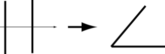
Figure 7: Eq. (3.7) maps a strip in the $(y,z)$ plane to a wedge in the $(Y,Z)$ plane

Notice that (3.8) is the metric derived by Polchinski and Witten [17] in the supersymmetric case, but for one notable difference: here the $Y$ direction is not compact. On the other hand, in the new coordinate system $(Y,Z)$ the periodicity under $y\to y+2\pi R$ reflects itself in the orbifold identification

$$Z+i\,Y\ \to\ e^{2\pi i\lambda R}\ (Z+i\,Y)\ ,$$ (3.9)

a two-dimensional rotation ${\cal R}_{\theta}$ in the $(Y,Z)$ plane by an angle $\theta=2\pi\lambda R$. In addition, the orientifold identification $y\rightarrow-y$ maps into a parity $\Pi_{Y}$ times a rotation ${\cal R}_{2\omega}$ by an angle $2\omega$, so that the new $\Omega$ projection is

$$\Omega^{\prime}\ =\ \Omega\ \Pi_{Y}\ {\cal R}_{2\omega}\ ,$$ (3.10)

where $\Omega$ denotes the conventional world-sheet parity. Notice that both the metric and the dilaton in (3.5) depend effectively on the real part of an analytic function, and thus generally on a pair of real variables, aside from the case of [17], where the function is a linear one, so that one of the real variables actually disappears. This simple observation explains the special role of the single-variable solution of [17] in this context.

As sketched in fig. 7, the exponential mapping turns the region delimited by the two parallel fixed lines of the orientifold operations in the $(y,z)$ plane into a wedge in the $(Y,Z)$ plane, delimited by the two lines

$$\Omega^{\prime}~{}:\ Y = \tan\omega\ Z\ ,$$

$$\Omega^{\prime}~{}{\cal R}_{2\pi\lambda R}:\ Y = \tan(\pi\lambda R+\omega)\ Z\ ,$$ (3.11)

so that the orientifolds and the branes at $y=0$ form an angle $\theta_{0}=\ \omega$ with the $Z$ axis, while those at $y=\pi R$ form an angle $\theta_{1}=\ \pi\lambda R+\omega$. Notice that the orbifold identification (3.9) implies that in general the two-dimensional $(Y,Z)$ plane contains singularities. In order to avoid subtleties of this type, in what follows we restrict our attention to a case where this complication is absent.

The example we have in mind is a variant of the M-theory breaking model of [22]. Its oriented closed part is related by a T-duality to a Scherk-Schwarz deformation of the toroidally compactified IIB spectrum of [22] (our conventions are spelled out in the reviews in [3]), described by

$$\mathcal{T} = (|V_{8}|^{2}+|S_{8}|^{2})\Lambda_{m,2n}+(|O_{8}|^{2}+|C_{8}|^{2})\Lambda_{m,2n+1}$$ (3.12)

$$- (V_{8}\bar{S}_{8}+S_{8}\bar{V}_{8})\Lambda_{m+1/2,2n}-(O_{8}\bar{C}_{8}+C_{8}\bar{O}_{8})\Lambda_{m+1/2,2n+1}\ .$$

Here the $\Lambda$’s are toroidal lattice sums, while the orientifold operation is based on $\Omega^{\prime}=\Omega\Pi_{1}$, with $\Pi_{1}$ the inversion along the circle, corresponding to the Klein-bottle amplitude

$$\mathcal{K}\ =\ \frac{1}{2}\,\left\{(V_{8}-S_{8})W_{2n}\ +\ (O_{8}-C_{8})W_{2n+1}\right\}\ ,$$ (3.13)

where the $W$’s are winding sums, and introduces an $O8_{+}$ plane at $y=0$ and an $\overline{O8}_{+}$ plane at $y=\pi R$. For consistency, these demand that no net $R-R$ charge be introduced, a condition met by N pairs of D8-$\overline{D8}$ branes, where the choice $N=16$ is singled out by the connection with M-theory [22]. A simple extension of the arguments in [23] shows that the unoriented closed spectrum described by (3.12) and (3.13) precisely interpolates between the type I string in the $R\rightarrow\infty$ limit and the type 0B orientifold with the tachyonic orientifold projection of [24], to be contrasted with the non-tachyonic $0^{\prime}B$ projection of [25], in the $R\rightarrow 0$ limit.

In order to obtain a classical configuration as in (3.5), without tachyons in the open sector, one can put the $N$ $\overline{D8}$ branes on top of the $O8_{+}$ planes and the $N$ $D8$ branes on top of the $\overline{O8}_{+}$ planes. This configuration differs from the one emphasized in [22] and related to the phenomenon of “brane supersymmetry”, with the $D8$ on top of the $O8_{+}$ and the $\overline{D8}$ on top of the $\overline{O8}_{+}$, by an overall interchange of the positions of branes and anti-branes. This has an important physical effect: whereas in the model of [22] both the $NS$-$NS$ tadpoles and the $R-R$ charges are locally saturated at the two endpoints, in this case there is a local unbalance of charges and tensions that results in an overall attraction between the endpoints driving the orientifold system toward a vanishing value for the radius $R$.

The resulting open string amplitudes

$$\mathcal{A} = \frac{N^{2}+M^{2}}{2}\ (V_{8}-S_{8})W_{n}+NM(O_{8}-C_{8})W_{n+1/2}\ ,$$

$$\mathcal{M} = -\frac{N+M}{2}\ \hat{V}_{8}W_{n}-\frac{N+M}{2}\hat{S}_{8}(-1)^{n}W_{n}\ ,$$ (3.14)

describe matter charged with respect to an $SO(N)\times SO(M)$ gauge group, where $N=M$ on account of the $R-R$ tadpole conditions, with nine-dimensional massless Majorana fermions in the symmetric representations ($N(N+1)/2$,1) and (1,$M(M+1)/2$) and massive fermions in the bi-fundamental representation ($N,M$). Notice that tachyons appear for small values of $R$. This spectrum should be contrasted with the one of [22] exhibiting “brane supersymmetry”, where the massless fermions are in antisymmetric representations. It is a simple exercise to evaluate tensions and $R-R$ charges at the two ends of the interval:

$$T_{0}\ =\ (N-16)T_{8}\ ,\qquad T_{1}\ =\ (N-16)T_{8}\ ,$$

$$q_{0}\ =\ -\,(N+16)T_{8}\ ,\qquad q_{1}\ =\ (N+16)T_{8}\ .$$ (3.15)

These translate into corresponding values for the parameters $\lambda$ and $\omega$ of the classical solution in (3.4), that in this case are

$$\lambda=\frac{1}{R}\ ,\quad\cos\omega=\frac{16-N}{16+N}\ .$$ (3.16)

Hence, in the new coordinate system (3.6) the orbifold operation (3.9) becomes a $2\pi$ rotation, and can thus be related to the fermion parity $(-1)^{F}$, while the orientifold operation $\Omega^{\prime}$ combines a world-sheet parity with a rotation. Notice also that $\lambda\pi R=\pi$, and therefore the $O_{+}$ and $\overline{O}_{+}$ planes are actually juxtaposed in the $(Y,Z)$ plane along the real axis $Y=0$, forming somehow a bound state with vanishing total $R-R$ charge. To be precise, the $O_{+}$ plane lies along the half-line $Y=0,$ $Z>0,$ while the ${\bar{O}}_{+}$ plane lies along the complementary half-line $Y=0,$ $Z<0.$ The end result is that in the $(Y,Z)$ plane one is describing the $0B$ (or $IIB/(-1)^{F}$) string, subject to the orientifold projection $\Omega^{\prime}=\Omega\Pi_{Y}$, where $Y,$ as already stressed, is here a noncompact coordinate. By our previous arguments, all this is somehow equivalent to the type IIB orientifold compactified on a circle that we started with. In more physical terms, the attraction between the sets of $D(\overline{D})$ branes and $O(\overline{O})$ planes at the ends of the interval drives them to collapse into suitable systems of $D$-branes and $O$-planes carrying no net $R-R$ charge, that should be captured by the static solutions of the effective action (3.1), and these suggest a relation to the $0B$ theory. In this respect, a potentially singular fate of space time opens the way to a sensible string vacuum. We would like to stress, however, that the picture supplied by the classical solution (3.5) is incomplete, since the origin $Y=Z=0$ is actually the site of a singularity. Indeed, the resulting $O$-plane system has no global $R-R$ charge, but has nonetheless a dipole structure: its $Z<0$ portion carries a positive charge, while its $Z>0$ portion carries a negative charge. While we are not able to provide more stringent arguments, it is reasonable to expect that the condensation of the open and closed-string tachyons emerging in the $R\to 0$ limit can drive a natural redistribution of the dipole charges between the two sides, with the end result of turning the juxtaposed $O$ and $\overline{O}$ into a charge-free type-$O$ orientifold plane. If this were the case, not only the resulting geometry of the bulk, but also the $D/O$ systems, would become those of the $0B$ string.

In order to provide further evidence for this, let us look more closely at the type 0B orientifold we identified, using the original ten-dimensional construction of [24]. The 0B torus amplitude is [28]

$$\mathcal{T} = (|O_{8}|^{2}+|V_{8}|^{2}+|S_{8}|^{2}+|C_{8}|^{2})\ ,$$ (3.17)

while the orientifold operation includes the parity $\Omega^{\prime}=\Omega\Pi_{Y}$, so that the Klein-bottle amplitude

$$\mathcal{K}=\frac{1}{2}\ \left(O_{8}+V_{8}-S_{8}-C_{8}\right)\$$ (3.18)

introduces an $O8$ plane at $Y=0$, without $R-R$ charge and with a tension that precisely matches that of the type-IIB $O8$-$\overline{O8}$ bound state. In general the type-0 orientifold planes, being bound states of IIB orientifold planes, have in fact twice their tension. In the present case, the parity $\Pi_{Y}$ along a noncompact coordinate sends one of the orientifold planes to infinity, with the net result of halving the total tension seen in the $(Y,Z)$ plane.

One can also add to this system two different types of brane-antibrane pairs, and the open-string amplitudes read [24]

$$\mathcal{A} = \frac{n_{o}^{2}+n_{v}^{2}+n_{s}^{2}+n_{c}^{2}}{2}\ V_{8}+(n_{o}n_{v}+n_{s}n_{c})\ O_{8}$$

$$- (n_{s}n_{v}+n_{c}n_{o})\ S_{8}-(n_{s}n_{o}+n_{c}n_{v})\ C_{8}\ ,$$

$$\mathcal{M} = -\ \frac{n_{v}+n_{o}+n_{s}+n_{c}}{2}\ \hat{V}_{8}\ ,\$$ (3.19)

while the corresponding $R-R$ tadpole conditions are

$$n_{o}\ =\ n_{v}=\ N\ ,\quad n_{s}\ =\ n_{c}=\ M\ .$$ (3.20)

The gauge group of this type-0 orientifold, $SO(N)^{2}\times SO(M)^{2}$, becomes remarkably similar to that of the type-II orientifold we started from, provided only branes of one type are present, together with the corresponding antibranes, a configuration determined setting for instance $M=0$. The resulting spectrum is then purely bosonic, and the precise statement is that, in the $R\rightarrow 0$ limit, the expected endpoint of the collapse, the spectrum of the type-II orientifold should match the purely bosonic spectrum of this type-0 orientifold, as was the case for their closed sectors. Actually, for the geometry of the $D/O$ configurations this was not totally evident, and the same is true for the open spectrum, due to an apparent mismatch in the fermionic content, but we would like to argue again that a proper account of tachyon condensation does justice to the equivalence.

The open-string tachyon $T_{ai}$ of the type-II orientifold is valued in the bi-fundamental, and therefore carries a pair of indices in the fundamental of the $SO(N)\times SO(N)$ gauge group. In the $R\rightarrow 0$ limit, all its Kaluza-Klein excitations acquire a negative mass squared. These tachyons will naturally condense, with $<T_{ai}>=T(y)\ \delta_{ai}$, where $T(y)$ denotes the tachyonic kink profile, breaking the gauge group to its diagonal $SO(N)$ subgroup, so that, after symmetry breaking and level by level, the fermions will fall in the representations

$$C^{(k+1/2)}~{}:\frac{N(N-1)}{2}+\frac{N(N+1)}{2}\ ,$$

$$S^{(2k)}~{}:\frac{N(N+1)}{2}\ ,\qquad S^{(2k+1)}~{}:\frac{N(N-1)}{2}\ .$$ (3.21)

In the $R\rightarrow 0$ limit the appropriate description of tachyon condensation is in the T-dual picture, and after a T-duality the interactions within the open sector must respect Kaluza-Klein number conservation. Therefore the Yukawa interactions, that before symmetry breaking are of the type

$$S_{(ij)}^{(2k)}C_{ja}^{t,(k+1/2)}T_{ai}^{(k-1/2)}\ ,\qquad S_{(ab)}^{(2k)}C_{bi}^{(k+1/2)}T_{ia}^{t,(k-1/2)}\ ,$$

$$S_{[ij]}^{(2k+1)}C_{ja}^{t,(k+1/2)}T_{ai}^{(k+1/2)}\ ,\qquad S_{[ab]}^{(2k+1)}C_{bi}^{(k+1/2)}T_{ia}^{t,(k+1/2)}\ ,$$ (3.22)

will give rise to the mass terms $S_{(ij)}C_{(ji)}$ , $S_{[ij]}C_{[ji]}$. The conclusion is that the final low-lying open spectra are bosonic on both sides and actually match precisely.

A more direct argument for the equivalence we are proposing would follow from a natural extension of Sen’s description of tachyon condensation [26]. As we have already stressed, the $O8$ and $\overline{O8}$ attract one another and drive the orientifold to a collapse. In the T-dual picture, the $O9$ and $\overline{O9}$ condense into a non-BPS orientifold plane in one lower dimension, that in the $R\rightarrow 0$ limit becomes the type-0 orientifold plane that we have described above. This type of phenomenon can plausibly be related to the closed-string tachyon non-trivial profile in this model, in a similar fashion to what happens for the open-string tachyon kink profile in $D$-$\overline{D}$ systems. At the same time, after T-duality the $D9$ and $\overline{D9}$ branes decay into non-BPS $D8$ branes via the appropriate tachyon kink profile. Due to the new $(-1)^{F}$ operation, these new non-BPS type-II branes match directly the non-BPS type-0 branes discussed in [24, 27], since the $(-1)^{F}$ operation removes the unwanted additional fermions. Let us stress that String Theory can resolve in this fashion the potential singularity associated to an apparent collapse of space time: after tachyon condensation, the $O$-$\overline{O}$ attraction can give birth to a well defined type-0 vacuum.

In this example one is confronted with the ideal situation in which a vacuum redefinition can be analyzed to some extent in String Theory. In general, however, a string treatment in such detail is not possible, and it is therefore worthwhile to take a closer look, on the basis of the intuition gathered from Field Theory, at how the conventional perturbative string setting can be adapted to systems in need of vacuum redefinitions, and especially at what it can teach us about the generic features of the redefinitions. We intend to return to this issue in a future publication [10].

3-b. Threshold corrections and $NS$-$NS$ tadpoles

While $NS$-$NS$ tadpoles ask for classical resummations that are very difficult to perform systematically, it is often possible to identify physical observables for which resummations are needed only at higher orders of perturbation theory. This happens whenever, in the appropriate limit of moduli space (infinite tube length, in the case of disk tadpoles), massless exchanges cannot be attached to the sources.

The one-loop finiteness of certain types of quantum corrections in models with broken supersymmetry and $NS$-$NS$ tadpoles was actually one of the original motivations for our work. One such example is provided by scalar (Wilson line) masses in brane-antibrane or brane supersymmetry breaking models . They can be simply computed from the vacuum energy turning on Wilson lines $\Lambda(a_{i})$, where $A=(e^{2\pi ia_{1}},e^{-2\pi ia_{1}},\cdots e^{2\pi ia_{16}},e^{-2\pi ia_{16}})$ denotes a collection of Wilson lines in a Cartan subalgebra of the $D$-brane gauge group under consideration, so that after T-dualities the $a_{i}$ can be related to $D$-brane displacements in the internal space, and the scalar mass matrix is then proportional to

$${\cal M}_{ij}^{2}={\partial^{2}\Lambda\over\partial a_{i}\partial a_{j}}\ .$$ (3.23)

Since the propagation of massless modes in the tree-level (transverse channel) description of (3.23) is insensitive to the $D$-brane positions $a_{i}$, only massive modes contribute to the mass matrix ${\cal M}_{ij}^{2}$. As a result, in this particular example the UV (IR in the tree-level channel) divergence would first manifest itself at genus $3/2$.

The threshold corrections to gauge couplings, defined by

$${4\pi^{2}\over g^{2}(\mu)}={4\pi^{2}\over g_{0}^{2}}+\Delta(\mu,\Phi_{i})\ ,$$ (3.24)

where $g_{0}$ is the tree-level gauge coupling, are a second interesting observable of this type. These corrections depend on the energy scale $\mu$ and also on the moduli fields $\Phi_{i}$ of the string model under consideration. We can now show that, in a large class of string constructions with $NS$-$NS$ tadpoles, including brane-antibrane pairs and brane supersymmetry breaking models, the one-loop threshold corrections are UV finite, despite the presence of tadpoles. We can also show that, at the one-loop order, the differences of gauge couplings for gauge groups related by Wilson line deformations $W$, $1/g^{2}(W)-1/g^{2}(0)$, quantities that are of direct relevance for unification purposes, are UV finite in any non-supersymmetric string model.

The first example that we would like to discuss is obtained adding N $D5-\overline{D5}$ pairs to the $T^{4}/Z_{2}$ orbifold of the type $I$ superstring [32]. If the additional $N$ $D5$ branes are placed, together with the original 32, at a given fixed point of the orbifold while the $N$ $\overline{D5}$ are placed at a different fixed point, that for simplicity we take to be separated only along one of the internal directions, the resulting gauge group is $U(16)_{9}\otimes[U(16+N)\otimes U(N)]_{5}$. The N pairs generate an $NS$-$NS$ tadpole localized in six dimensions, that would be expected to introduce UV divergences in one-loop threshold corrections.

In order to obtain a field-theory interpretation, one can turn windings into momenta via a pair of $T$-dualities that also convert $D9$ and $D5$ branes into $D7$ and $D3$. Using the background field construction of [31], the one-loop threshold corrections for the ${D3}$ gauge couplings are then found to be [10]

$$\Delta = -\ \frac{4}{v_{3}}\,({\rm Tr}\,Q^{2})\int_{0}^{\infty}\,dl\,(P^{(2)}-P_{e}^{(2)})\$$ (3.25)

$$- (TrQ^{2})\,{N\over 2^{8}\pi^{2}v_{1}v_{2}v_{3}}\int_{0}^{\infty}dl\,{\vartheta_{2}^{4}\over\eta^{12}}\,\left({2\pi^{2}\over 3}+{\vartheta_{2}^{{}^{\prime\prime}}\over\vartheta_{2}}-{\vartheta_{1}^{{}^{\prime\prime\prime}}\over 6\pi\eta^{3}}\right)\,(-1)^{m}P^{(2)}P^{(4)}\,,$$

where $Q$ is a gauge generator for the $D3$ gauge group, $v_{1},v_{2},v_{3}$ are the volumes of the three internal tori, $P^{(2)}$ and $P^{(4)}$ are Kaluza-Klein momentum sums along the torus where the T-duality was performed and along the other two tori, respectively, $P_{e}^{(2)}$ is a corresponding even momentum sum, and $\eta$ and $\vartheta_{i}$ are Jacobi functions. The non-supersymmetric contribution in the second line of (3.25) is IR and UV finite. The UV finiteness can be explained from the supergravity point of view, and we shall return to it below, while the IR finiteness is guaranteed by the separation between the $D3$ and the $\overline{D3}$ in the internal space. In the field theory (large volume) limit the non-supersymmetric contribution is negligible, while the explicit evaluation of the first term in (3.25) was done in [31] and gives

$$\Delta\ =\ -\ {1\over 4}\ b^{({\cal N}=2)}\ln({\sqrt{G}\mu^{2}|\eta(U)|^{4}{\rm Im}U})\ ,$$ (3.26)

where for a rectangular torus of radii $R_{1},R_{2}$, $\sqrt{G}=R_{1}R_{2}$ and ${\rm Im}U=R_{1}/R_{2}$. In (3.26), $b^{({\cal N}=2)}$ denote beta function coefficients for Kaluza-Klein excitations in the compact torus where the T-dualities were performed, that fill ${\cal N}=2$ multiplets. The first, BPS-like contribution in (3.25), is similar to the standard ${\cal N}=2$ one in orientifold models [31], and is finite. The non-supersymmetric one originates from the cylinder and reflects the $D3-\overline{D3}$ interaction between branes and antibranes located at different orbifold fixed points. This explains, in particular, the origin of the alternating factor $(-1)^{m}$. The remarkable property of (3.25) is that the threshold corrections are UV finite, despite the presence of the $NS$-$NS$ tadpole. This can be understood noting that in the $l\rightarrow\infty$ limit the string amplitudes acquire a field-theory interpretation in terms of dilaton and graviton exchanges between $Dp$-branes and $Op$-planes. For parallel localized sources, the relevant terms in the effective Lagrangian are

$$S = \frac{1}{2k^{2}}\int d^{10}x\sqrt{-G}\biggl{\{}R-\frac{1}{2}(\partial\varphi)^{2}-\frac{1}{2(p+2)~{}!}e^{(5-p-2)\varphi/2}F_{p+2}^{2}\biggr{\}}$$ (3.27)

$$- \int_{{\bf y}={\bf y_{i}}}d^{p+1}\xi\biggl{\{}\sqrt{-\gamma}\left[T_{p}e^{(p-3)\varphi/4}+e^{(p-7)\varphi/4}{\rm tr\,}F_{\mu\nu}^{2}\right]+qC^{(p+1)}\biggr{\}}\ ,$$

where ${\bf\xi}$ are brane world-volume coordinates, $q=\pm 1$ distinguishes between branes or $O$-planes and antibranes or $\overline{O}$-planes, $G$ is the 10-dimensional metric, $\gamma$ is the induced metric and $C^{(p+1)}$ denotes a $R$-$R$ form that couples to the branes. The final result for the corrections to gauge couplings, obtained using (3.27) while treating for simplicity the K-K momenta as a continuum, is proportional to

$$T_{p}\int\frac{d^{9-p}k}{(2\pi)^{9-p}}\biggl{\{}-T^{\mu\nu}\,\langle h_{\mu\nu}h_{\rho\sigma}\rangle\,\eta^{\rho\sigma}\ +\ {\rm tr\,}F^{2}\langle\,\varphi\varphi\rangle\,\frac{(p-3)(p-7)}{16}\biggr{\}}\ ,$$ (3.28)

where

$$\langle h_{\mu\nu}h_{\rho\sigma}\rangle\ =\ \frac{1}{k^{2}}\left(\eta_{\mu\rho}\eta_{\nu\sigma}+\eta_{\mu\sigma}\eta_{\nu\rho}-\frac{1}{4}\eta_{\mu\nu}\eta_{\rho\sigma}\right)$$ (3.29)

is the ten-dimensional graviton propagator in de Donder gauge,

$$\langle\varphi\varphi\rangle\ =\ \frac{1}{k^{2}}$$ (3.30)

is the ten-dimensional dilaton propagator, and

$$T_{\mu\nu}={\rm tr\,}\left(F_{\mu\rho}F_{\nu}^{\rho}-\frac{1}{4}\eta_{\mu\nu}F^{2}\right)$$ (3.31)

is the vector energy-momentum tensor. Irrespective of the dilaton tadpole, it can be verified that the dilaton and graviton exchanges in (3.28) cancel precisely, source by source, in the threshold corrections, ensuring that the result is actually finite. Notice that this type of supergravity argument applies to a large class of string models, including the non-tachyonic type $0^{\prime}B$ orientifold and its orbifolds [25].

A second and similar example to this effect is provided by the brane supersymmetry breaking model proposed in [4, 5], that contains 32 $D9$ and 32 $\overline{D5}$ branes, for simplicity at the origin of the internal space, $O9_{+}$ and 16 $O5_{-}$ orientifold planes, so that supersymmetry is broken at the string scale on the $\overline{D5}$. The main difference with respect to the previous example is that the model is tachyon-free for any position of the antibranes in the compact space. In order to display the decoupling of the tadpole, let us take for simplicity all internal dimensions to be transverse to the antibranes, a setting that can be realized performing a pair of T-dualities in the model of [5], that would turn the $\overline{D5}$ branes into $\overline{D3}$ and the $D9$ branes into $D7$. In this case, the one-loop threshold corrections for the $\overline{D3}$ gauge couplings are found to be [10]

$$\Delta = -\,\frac{4}{v_{3}}(TrQ^{2})\int_{0}^{\infty}\ dl\ (P^{(2)}-P_{e}^{(2)})\$$ (3.32)

$$- (TrQ^{2})\ {1\over 8\pi^{2}v_{1}v_{2}v_{3}}\int_{0}^{\infty}dl\ {\vartheta_{2}^{4}\over\eta^{12}}\,\left({2\pi^{2}\over 3}+{\vartheta_{2}^{{}^{\prime\prime}}\over\vartheta_{2}}-{\vartheta_{1}^{{}^{\prime\prime\prime}}\over 6\pi\eta^{3}}\right)\ P_{e}^{(4)}P_{e}^{(2)}\ .$$

The second, non-supersymmetric contribution to (3.32), originates from the Möbius amplitude, but clearly the combinations of terms appearing in (3.25) and (3.32), and actually in any similar computation, are the same. In this example, the non-supersymmetric contribution in the second line of (3.32) is IR divergent, reflecting the presence of massless open-string states in the sector that induces the breaking of supersymmetry. The explicit evaluation of (3.32) gives

$$\Delta\ =\ {1\over 4}\ b^{({\cal N}=0)}\,\ln{M_{s}^{2}\over\mu^{2}}\ -\ {1\over 4}\ b^{({\cal N}=2)}\ln({\sqrt{G_{i}}\mu^{2}|\eta(U)|^{4}{\rm Im}U})\ ,$$ (3.33)

where $M_{s}$ is the string scale and the non-supersymmetric contribution was here evaluated in the field theory limit, and where $b^{({\cal N}=0)}$ denotes the contribution from the supersymmetry breaking sector, so that the total beta function of the model is

$$b\ =\ b^{({\cal N}=0)}\ +\ b^{({\cal N}=2)}\ =\ 3\ .$$ (3.34)

Notice also that, in the limit where the internal volume transverse to the $\overline{D3}$ is large, the second term in (3.25) and the term in the second line of (3.32) that is most relevant as $l\to\infty$ become negligibly small compared to the standard contribution from the supersymmetry breaking sector. The threshold corrections are then dominated by the first terms, that are precisely given by the standard supersymmetric expressions [31], where only the would-be BPS winding states contribute and the string oscillators decouple. Therefore, at the one-loop level, despite the breaking of supersymmetry at the string scale on the antibranes, the threshold corrections are essentially determined by a supersymmetric contribution. This result confirms the conjecture, made in [5], that in brane-antibrane pairs and in brane supersymmetry breaking models threshold corrections in codimension larger than two are essentially given by supersymmetric expressions, due to the supersymmetry of the bulk (closed string) spectrum. Another example of this type is provided by a stack of $D$ branes at orbifold singularities, where the orbifold action on the Chan-Paton factors breaks the gauge group to $SU(3)\otimes SU(2)\otimes U(1)$.

As observed in [33], the one-loop threshold corrections are not UV finite in models with intersecting branes [7]. The supergravity argument in the previous Section fails in this case since the sources ($D$-branes and $O$-planes) present in the compact space are not parallel. Since the brane couplings to bulk fields depend on their spin, the cancellations that we have described for the case of parallel branes/orientifolds cease to occur. However, differences of gauge couplings for gauge groups related by Wilson line breakings $W$, $1/g^{2}(W)-1/g^{2}(0)$, quantities that are of direct relevance for unification purposes, are still UV finite at one-loop, as can be seen from general arguments and will be verified explicitly in [10].

4. Conclusions

Our analysis of tadpoles in Field Theory shows that the endpoint of the classical resummation flow is an extremum of the effective potential, but not necessarily a minimum. In addition, the flow should occur without touching any inflection points, where the resummation procedure breaks down. In the $\phi^{4}$ example, however, we found the peculiar initial points $\phi_{0}=-v/2$, where $v$ are the extrema of the scalar potential, such that only the first terms in the tadpole expansions contribute and the flows terminate at the endpoints $\langle\phi\rangle=v$ on the other side of the potential barrier. Using the link with Newton’s tangent method, we have also associated to this effect a geometrical interpretation: this occurs whenever the tangent to the derivative of the potential, $V^{\prime}$, at the initial “wrong vacuum”, crosses the real axis exactly at an extremum. For the last example considered in Section 2-b one of these points, for small values of the “magnetic field” $c$, lies well within the convergence region of tadpole resummations, so that the effect is perturbative. If this finding were to generalize, one could conceive carrying out the resummation program to the very end both in Field Theory and in String Theory starting from neighborhoods of such points. Simple resummations have been performed explicitly in toy models with localized branes, that affect the bulk fields via boundary conditions, and we have presented an explicit example where a toy model for gravity is taken into account at the first two lowest orders, with a graviton mass term in the wrong vacuum that is not of Fierz-Pauli type, so that a ghost is present in the spectrum, while it is of Fierz-Pauli type in the proper vacuum. Tadpole resummations in the wrong vacuum suffice even in this case to recover the correct results for physical observables.

At the string level, we have provided some evidence for an example of explicit vacuum redefinitions connecting a type-$II$ orientifold with $NS$-$NS$ tadpoles to its correct vacuum, that can be related to a type-0 orientifold. We then showed that, despite the presence of $NS$-$NS$ tadpoles, one-loop threshold corrections are UV finite in a large class of string models with broken supersymmetry, including brane-antibrane pairs, brane supersymmetry breaking models and essentially any type-$II$ or type-0 orientifolds with no closed string tachyons (that would introduce additional divergences in the threshold corrections) containing parallel BPS or non-BPS brane/orientifold configurations.

The UV finiteness of the one-loop results presented in Section 3 would seem to imply that the threshold corrections are insensitive to large tadpoles. This conclusion, however, is likely to be incorrect, since the one-loop finiteness was the result of a delicate cancellation between dilaton and graviton exchanges in the tree-level closed string amplitude. This cancellation is not expected to be preserved at higher orders, and taking into account the proper resummations appears to spoil perturbation theory, yielding a result that, due to the non-analyticity in the dilaton mass, is of the same order as the tree-level disk contribution.

Starting with genus $3/2$ amplitudes [34], Dyson resummations of the propagators are clearly necessary. For example, the higher-genus contributions to Wilson-line masses, normalized to the one-loop (annulus and Möbius) contribution are of order

$$\frac{(\frac{i}{-V^{\,\prime\prime}})^{2}\,(-iV^{\,\prime})\,(-iV^{\,\prime\prime\prime}_{m00})\,\frac{i}{-m^{2}}\,(-iV^{\,\prime})}{\frac{i}{-m^{2}}\,(-iV^{\,\prime})}\ =\ \frac{V^{\,\prime\prime\prime}_{m00}}{V^{\,\prime\prime}}\,\frac{V^{\,\prime}}{V^{\,\prime\prime}}\ ,$$ (4.1)

where we considered for definiteness a higher-order string amplitude whose field theory limit would contain three closed string propagators, two massless and one massive and one cubic disk vertex. In (4.1), $m^{2}$ denotes the mass of the lowest Kaluza-Klein excitations and $V^{\,\prime\prime\prime}_{m00}$ denotes the disk three point function for one massive and two massless closed string fields. Higher-order resummations in this particular example would thus be perturbative in the tadpole only if

$$\left|V^{\,\prime\prime\prime}_{m00}V^{\,\prime}/(V^{\,\prime\prime})^{2}\right|<<1\ .$$ (4.2)

This condition is not satisfied by the exponential scalar potential of String Theory, and therefore formally higher-order contributions would give rise in this case to ${\cal O}(1)$ corrections to the one-loop result. As argued in Section 2-d, however, for codimension larger than two tadpoles effectively decouple from the moduli of the transverse space. If, as in the examples discussed in Section 3, there are additional contributions from states propagating in only one or two transverse dimensions that do not couple to the tadpole to leading order, these are expected to provide the main contributions to Wilson-line masses or threshold corrections, that are reliably computed in string perturbation theory. The dependence on the moduli corresponding to parallel dimensions, on the other hand, does not decouple.

Concerning the gauge couplings, in the class of models discussed in Section 3 the one-loop corrections are UV finite. In any non-supersymmetric model (for instance in intersecting brane models [7]), only massive states contribute to differences of gauge couplings for gauge groups related by Wilson-line deformations $W$, $\Delta(W)\equiv 1/g^{2}(W)-1/g^{2}(0)$, the relevant quantities for unification purposes in Wilson-line GUT breaking models. Consequently, no tadpole divergences manifest themselves in these quantities at one loop. In this case, even at higher genus, closed-string propagators attached to external gauge field lines contain only massive states. In particular, the genus $3/2$ contribution, when compared to the one-loop one, is proportional to $V^{{}^{\prime\prime}}_{0m}/V^{{}^{\prime\prime}}$, and is therefore renormalizing the one-loop correction coming from the second, tadpole dependent term in (3.25). By the previous arguments, for codimension larger than two these terms are negligible compared to the first term given by the standard supersymmetric expressions [31], to which only BPS-like states contribute. In principle, the contributions of parallel dimensions do not decouple, and therefore the dependence on their moduli is not determined reliably by computations in the wrong Minkowski vacuum.

The resummation program that we have initiated in this paper can be of practical use if the endpoint of the resummation flow is a local minimum of the theory. As we saw in Section 2-b, this is not always the case, since depending on the starting point a resummation may well end at a local maximum of the effective potential or may even not converge at all. Therefore, an important constraint for tadpole resummations is to start in an appropriate region, which in String Theory restricts, in particular, the values of the string coupling. Finally, if non-renormalization points like those we encountered in Section 2-b were to exist in a perturbative region and within the convergence radius, “wrong” vacua close to them could lead to significant simplifications and could make resummations not only conceptually important, but also of real practical use. A proper extension of these resummation procedures to String Theory must cope with a number of additional subtleties that are typical of string amplitudes, and is therefore left for future work [10].

Appendix A Mixed propagators

Let us consider the ${\cal D}$-dimensional action

$$S\ = \ \int d^{\mathcal{D}}x\left[\frac{1}{2}h^{\rho\sigma}\square h_{\rho\sigma}-h^{\rho\sigma}\partial_{\sigma}\partial^{\mu}h_{\rho\mu}+h^{\rho\sigma}\partial_{\rho}\partial_{\sigma}h-\frac{1}{2}h\square h+\frac{m^{2}}{2}\left(h_{\rho\sigma}h^{\rho\sigma}-ah^{2}\right)\right]$$ (A1)

$$+ \int d^{\mathcal{D}}x\left[\frac{1}{2}\varphi\left(\square-M^{2}\right)\varphi+2b\varphi h\right]\ ,$$

obtained expanding up to the quadratic order the tadpole potential (2.106), that is also the quadratic part of the linearized Einstein-Hilbert action coupled to a massive scalar field, aside from the mass term for the graviton, that is taken to be of general form. To compute the propagators, one must invert the kinetic operator

$$\left(\begin{array}[]{cc}G_{\mu\nu,\rho\sigma}^{-1}&-2ib\ \eta_{\mu\nu}\\ -2ib\ \eta_{\rho\sigma}&i(p^{2}+M^{2})\\ \end{array}\right)\ ,$$

where

$$G_{\mu\nu,\rho\sigma}^{-1} = \frac{i}{2}[(\eta_{\mu\rho}\eta_{\nu\sigma}+\eta_{\mu\sigma}\eta_{\nu\rho})(p^{2}-m^{2})-2\eta_{\mu\nu}\eta_{\rho\sigma}(p^{2}-am^{2})$$ (A2)

$$- \eta_{\mu\rho}p_{\nu}p_{\sigma}-\eta_{\mu\sigma}p_{\nu}p_{\rho}-\eta_{\nu\rho}p_{\mu}p_{\sigma}-\eta_{\nu\sigma}p_{\mu}p_{\rho}+2\eta_{\mu\nu}p_{\rho}p_{\sigma}+2\eta_{\rho\sigma}p_{\mu}p_{\nu}]\ .$$

The graviton propagator $G_{\mu\nu}$, the dilaton propagator $G_{\phi\phi}$ and the mixed propagator $G_{\mu\nu,\phi}$ can be obtained solving the system

$$G_{\alpha\beta,\mu\nu}G^{-1\mu\nu,\rho\sigma}\ -\ 2ibG_{\alpha\beta,\phi}\eta^{\rho\sigma} = \frac{1}{2}\ (\delta^{\rho}_{\alpha}\delta^{\sigma}_{\beta}\ +\ \delta^{\sigma}_{\alpha}\delta^{\rho}_{\beta})\ ,$$

$$-2b\eta^{\mu\nu}G_{\alpha\beta,\mu\nu}\ +\ (p^{2}+M^{2})G_{\alpha\beta,\phi} = 0\ ,$$

$$G_{\mu\nu,\phi}G^{-1\mu\nu,\rho\sigma}\ -\ 2ib\eta^{\rho\sigma}G_{\phi\phi} = 0\ ,$$

$$-2bG_{\mu\nu,\phi}\eta^{\mu\nu}+(p^{2}+M^{2})G_{\phi\phi} = -\,i\ .$$ (A3)

One can readily fix the general form of the propagators,

$$G_{\alpha\beta,\mu\nu} = A[\eta_{\alpha\mu}\eta_{\beta\nu}+\eta_{\alpha\nu}\eta_{\beta\mu}+B\ \eta_{\alpha\beta}\eta_{\mu\nu}+C(p_{\alpha}p_{\mu}\eta_{\beta\nu}+p_{\alpha}p_{\nu}\eta_{\beta\mu}+p_{\beta}p_{\mu}\eta_{\alpha\nu}+p_{\beta}p_{\nu}\eta_{\alpha\mu})$$ (A4)

$$+ D(p_{\alpha}p_{\beta}\eta_{\mu\nu}+p_{\mu}p_{\nu}\eta_{\alpha\beta})+Ep_{\alpha}p_{\beta}p_{\mu}p_{\nu}]\ ,$$

$$G_{\alpha\beta,\phi} = F\ \eta_{\alpha\beta}+G\ \frac{p_{\alpha}p_{\beta}}{m^{2}}\ ,$$ (A5)

$$G_{\phi\phi} = H\ ,$$ (A6)

and the solution is finally

$$A = -\ \frac{i}{2(p^{2}-m^{2})}\ ,\qquad B\ =\ \frac{2}{{\mathcal{D}}-2}\ \left[-1+\frac{(p^{2}+M^{2})(1-2a)m^{2}+8b^{2}}{\mathcal{Q}}\right]\ ,$$

$$C = -\frac{1}{m^{2}}\ ,\qquad D\ =\ \frac{2}{\cal Q}\left[(p^{2}+M^{2})(1-2a)+\frac{8b^{2}}{m^{2}}\right]\ ,$$

$$E = \frac{{\mathcal{D}}-2}{m^{2}}\ D\ ,\qquad F\ =\ \frac{2ib}{\mathcal{Q}}\ ,$$

$$G = \frac{2ib({\mathcal{D}}-2)}{\mathcal{Q}}\ ,\qquad H\ =\ -\,i\ \frac{p^{2}(1-a)({\mathcal{D}}-2)+m^{2}(1-a{\mathcal{D}})}{\mathcal{Q}}\ ,$$ (A7)

where the denominator is

$$\mathcal{Q}\ =\ (p^{2}+M^{2})\ [p^{2}(1-a)({\mathcal{D}}-2)+m^{2}(1-a{\mathcal{D}})]+\frac{4b^{2}}{m^{2}}\ [p^{2}({\mathcal{D}}-2)+{\mathcal{D}}m^{2}]\ .$$ (A8)

Acknowledgements We are very grateful to M. Berg, who collaborated with us at the early stages of this research and contributed most of the figures. We also benefitted from discussions with C. Angelantonj, D. Anselmi, C. Bachas, C. Becchi, G. Gabadadze, J. Magnen, J. Mourad, G. Passarino, M. Porrati, Ya.S. Stanev, and especially with I. Antoniadis. The work of E.D. was supported in part by the EU contract HPRN-CT-2000-00148, by the CNRS PICS no. 2530 and by the EU Excellence Grant MEXT-CT-2003-509661, while the work of M.N., G.P. and A.S. was supported in part by INFN, by the EU contracts HPRN-CT-2000-00122 and HPRN-CT-2000-00148, by the MIUR-COFIN contract 2003-023852, by the INTAS contract 03-51-6346 and by the NATO grant PST.CLG.978785. The authors are grateful to the CERN Theory Department, to the Scuola Normale Superiore of Pisa, to the CPhT of the École Polytechnique, to the Physics Department of the University of Rome “Tor Vergata” and to the Aspen Center for Physics for the hospitality extended to them at several stages of the present work.

References

- [1] J. Polchinski and Y. Cai, Nucl. Phys. B 296 (1988) 91; M. Bianchi and J. F. Morales, JHEP 0003 (2000) 030 [arXiv:hep-th/0002149].
- [2] W. Fischler and L. Susskind, Phys. Lett. B 171 (1986) 383, Phys. Lett. B 173 (1986) 262. See also: S. R. Das and S. J. Rey, Phys. Lett. B 186 (1987) 328.
- [3] A. Sagnotti, in Cargese ’87, “Non-Perturbative Quantum Field Theory”, eds. G. Mack et al (Pergamon Press, 1988), p. 521, arXiv:hep-th/0208020; G. Pradisi and A. Sagnotti, Phys. Lett. B 216 (1989) 59; P. Horava, Nucl. Phys. B 327 (1989) 461, Phys. Lett. B 231 (1989) 251; M. Bianchi and A. Sagnotti, Phys. Lett. B 247 (1990) 517, Nucl. Phys. B 361 (1991) 519; M. Bianchi, G. Pradisi and A. Sagnotti, Nucl. Phys. B 376 (1992) 365; For reviews see: E. Dudas, Class. Quant. Grav. 17, (2000) R41 [arXiv:hep-ph/0006190]; C. Angelantonj and A. Sagnotti, Phys. Rept. 371 (2002) 1 [Erratum-ibid. 376 (2003) 339] [arXiv:hep-th/0204089].
- [4] S. Sugimoto, Prog. Theor. Phys. 102 (1999) 685 [arXiv:hep-th/9905159].
- [5] I. Antoniadis, E. Dudas and A. Sagnotti, Phys. Lett. B 464 (1999) 38 [arXiv:hep-th/9908023]; C. Angelantonj, Nucl. Phys. B 566 (2000) 126 [arXiv:hep-th/9908064]; G. Aldazabal and A. M. Uranga, JHEP 9910 (1999) 024 [arXiv:hep-th/9908072]; C. Angelantonj, I. Antoniadis, G. D’Appollonio, E. Dudas and A. Sagnotti, Nucl. Phys. B 572 (2000) 36 [arXiv:hep-th/9911081].
- [6] G. Aldazabal, L. E. Ibanez and F. Quevedo, JHEP 0001 (2000) 031 [arXiv:hep-th/9909172]; D. Berenstein, V. Jejjala and R. G. Leigh, Phys. Rev. Lett. 88 (2002) 071602 [arXiv:hep-ph/0105042].
-
[7]
Some related contributions are:
C. Bachas, arXiv:hep-th/9503030; M. Berkooz, M. R. Douglas and R. G. Leigh, Nucl. Phys. B 480 (1996) 265 [arXiv:hep-th/9606139]; N. Ohta and P. K. Townsend, Phys. Lett. B 418 (1998) 77 [arXiv:hep-th/9710129]; R. Blumenhagen, L. Gorlich and B. Kors, Nucl. Phys. B 569 (2000) 209 [arXiv:hep-th/9908130], JHEP 0001 (2000) 040 [arXiv:hep-th/9912204]; G. Pradisi, Nucl. Phys. B 575 (2000) 134 [arXiv:hep-th/9912218]; R. Blumenhagen, L. Goerlich, B. Kors and D. Lust, JHEP 0010 (2000) 006 [arXiv:hep-th/0007024]; C. Angelantonj, I. Antoniadis, E. Dudas and A. Sagnotti, Phys. Lett. B 489 (2000) 223 [arXiv:hep-th/0007090]; C. Angelantonj and A. Sagnotti, arXiv:hep-th/0010279; G. Aldazabal, S. Franco, L. E. Ibanez, R. Rabadan and A. M. Uranga, JHEP 0102 (2001) 047 [arXiv:hep-ph/0011132]; M. Cvetic, G. Shiu and A. M. Uranga, Nucl. Phys. B 615 (2001) 3 [arXiv:hep-th/0107166]; C. Kokorelis, JHEP 0209, 029 (2002) [arXiv:hep-th/0205147]; D. Bailin, G. V. Kraniotis and A. Love, Phys. Lett. B 553 (2003) 79 [arXiv:hep-th/0210219]; G. Honecker, Nucl. Phys. B 666, 175 (2003) [arXiv:hep-th/0303015]; M. Larosa and G. Pradisi, Nucl. Phys. B 667 (2003) 261 [arXiv:hep-th/0305224]. - [8] R. Rohm, Nucl. Phys. B 237 (1984) 553; C. Kounnas and M. Porrati, Nucl. Phys. B 310 (1988) 355; I. Antoniadis, C. Bachas, D. C. Lewellen and T. N. Tomaras, Phys. Lett. B 207 (1988) 441; S. Ferrara, C. Kounnas, M. Porrati and F. Zwirner, Nucl. Phys. B 318 (1989) 75; C. Kounnas and B. Rostand, Nucl. Phys. B 341 (1990) 641; I. Antoniadis, Phys. Lett. B 246 (1990) 377; I. Antoniadis and C. Kounnas, Phys. Lett. B 261 (1991) 369; E. Kiritsis and C. Kounnas, Nucl. Phys. B 503 (1997) 117 [arXiv:hep-th/9703059].
- [9] J. Scherk and J. H. Schwarz, Nucl. Phys. B 153 (1979) 61; E. Cremmer, J. Scherk and J. H. Schwarz, Phys. Lett. B 84 (1979) 83; P. Fayet, Phys. Lett. B 159, 121 (1985).
- [10] M. Berg, E. Dudas, M. Nicolosi, G. Pradisi and A. Sagnotti, work in progress.
- [11] For a review see, for instance, J. P. Blaizot and E. Iancu, Phys. Rept. 359 (2002) 355 [arXiv:hep-ph/0101103].
- [12] M. Peskin and D.V. Schroeder, An Introduction to Quantum Field Theory (Reading, Addison-Wesley, 1995); W. Siegel, “Fields,” arXiv:hep-th/9912205.
- [13] S. B. Giddings, S. Kachru and J. Polchinski, Phys. Rev. D 66 (2002) 106006 [arXiv:hep-th/0105097]; S. Kachru, M. B. Schulz and S. Trivedi, JHEP 0310 (2003) 007 [arXiv:hep-th/0201028]; S. Kachru, R. Kallosh, A. Linde and S. P. Trivedi, Phys. Rev. D 68 (2003) 046005 [arXiv:hep-th/0301240]; R. Blumenhagen, D. Lust and T. R. Taylor, fluxes,” Nucl. Phys. B 663, 319 (2003) [arXiv:hep-th/0303016]; J. F. G. Cascales and A. M. Uranga, JHEP 0305, 011 (2003) [arXiv:hep-th/0303024]; M. Grana, T. W. Grimm, H. Jockers and J. Louis, Nucl. Phys. B 690, 21 (2004) [arXiv:hep-th/0312232]; F. Marchesano and G. Shiu, arXiv:hep-th/0408059; P. G. Camara, L. E. Ibanez and A. M. Uranga, arXiv:hep-th/0408036.
- [14] S. R. Coleman and E. Weinberg, Phys. Rev. D 7 (1973) 1888; R. Jackiw, Phys. Rev. D 9 (1974) 1686.
- [15] K. R. Dienes, E. Dudas and T. Gherghetta, Phys. Rev. D 62 (2000) 105023 [arXiv:hep-ph/9912455]; J. A. Bagger, F. Feruglio and F. Zwirner, Phys. Rev. Lett. 88 (2002) 101601 [arXiv:hep-th/0107128], JHEP 0202 (2002) 010 [arXiv:hep-th/0108010].
- [16] See, for instance, E. Whittaker and G.N. Watson, “A Course of Modern Analysis” (Cambridge, Cambridge Univ. Press).
- [17] J. Polchinski and E. Witten, Nucl. Phys. B 460 (1996) 525 [arXiv:hep-th/9510169].
- [18] I. Antoniadis and C. Bachas, Phys. Lett. B 450 (1999) 83 [arXiv:hep-th/9812093].
- [19] E. Dudas and J. Mourad, Nucl. Phys. B 575 (2000) 3 [arXiv:hep-th/9911019]; E. Accomando, I. Antoniadis and K. Benakli, Nucl. Phys. B 579, 3 (2000) [arXiv:hep-ph/9912287]; S. Cullen, M. Perelstein and M. E. Peskin, Phys. Rev. D 62, 055012 (2000) [arXiv:hep-ph/0001166].
- [20] H. van Dam and M. J. G. Veltman, Nucl. Phys. B 22 (1970) 397; V.I. Zakharov, JETP Lett. 12 (1970) 312; M. Porrati, Phys. Lett. B 534, 209 (2002) [arXiv:hep-th/0203014].
- [21] E. Dudas, J. Mourad and C. Timirgaziu, Nucl. Phys. B 660 (2003) 3 [arXiv:hep-th/0209176], JCAP 0403 (2004) 005 [arXiv:hep-th/0309057]; E. Dudas and C. Timirgaziu, JHEP 0403 (2004) 060 [arXiv:hep-th/0401201].
- [22] I. Antoniadis, E. Dudas and A. Sagnotti, Nucl. Phys. B 544 (1999) 469 [arXiv:hep-th/9807011]; I. Antoniadis, G. D’Appollonio, E. Dudas and A. Sagnotti, Nucl. Phys. B 553 (1999) 133 [arXiv:hep-th/9812118], Nucl. Phys. B 565 (2000) 123 [arXiv:hep-th/9907184].
- [23] J. D. Blum and K. R. Dienes, Nucl. Phys. B 516 (1998) 83 [arXiv:hep-th/9707160].
- [24] M. Bianchi and A. Sagnotti (1990), in [3].
- [25] A. Sagnotti, arXiv:hep-th/9509080, Nucl. Phys. Proc. Suppl. 56B (1997) 332 [arXiv:hep-th/9702093]; C. Angelantonj, Phys. Lett. B 444 (1998) 309 [arXiv:hep-th/9810214]; R. Blumenhagen, A. Font and D. Lust, Nucl. Phys. B 558 (1999) 159 [arXiv:hep-th/9904069].
- [26] A. Sen, JHEP 9808 (1998) 012 [arXiv:hep-th/9805170], arXiv:hep-th/9904207.
- [27] E. Dudas, J. Mourad and A. Sagnotti, Nucl. Phys. B 620, 109 (2002) [arXiv:hep-th/0107081].
- [28] L. J. Dixon and J. A. Harvey, Nucl. Phys. B 274 (1986) 93; N. Seiberg and E. Witten, Nucl. Phys. B 276 (1986) 272.
- [29] I. Antoniadis, K. Benakli and A. Laugier, Nucl. Phys. B 631 (2002) 3 [arXiv:hep-th/0111209].
- [30] I. Antoniadis, K. Benakli and M. Quiros, Nucl. Phys. B 583 (2000) 35 [arXiv:hep-ph/0004091].
- [31] C. Bachas and C. Fabre, Nucl. Phys. B 476 (1996) 418 [arXiv:hep-th/9605028]; I. Antoniadis, C. Bachas and E. Dudas, Nucl. Phys. B 560 (1999) 93 [arXiv:hep-th/9906039]; P. Bain and M. Berg, JHEP 0004 (2000) 013 [arXiv:hep-th/0003185].
- [32] M. Bianchi and A. Sagnotti (1991), in [3]; E. G. Gimon and J. Polchinski, Phys. Rev. D 54 (1996) 1667 [arXiv:hep-th/9601038].
- [33] D. Lust and S. Stieberger, arXiv:hep-th/0302221; D. Lust, P. Mayr, R. Richter and S. Stieberger, Nucl. Phys. B 696, 205 (2004) [arXiv:hep-th/0404134].
- [34] M. Bianchi and A. Sagnotti, Phys. Lett. B 211 (1988) 407, Phys. Lett. B 231 (1989) 389; I. Antoniadis and T. R. Taylor, Nucl. Phys. B 695, 103 (2004) [arXiv:hep-th/0403293].
- [35] A. Hebecker and A. Westphal, Annals Phys. 305 (2003) 119 [arXiv:hep-ph/0212175], arXiv:hep-th/0407014.