hep-th/0410103

Tachyon Dynamics in Open String Theory

Ashoke Sen

Harish-Chandra Research Institute

Chhatnag Road, Jhusi, Allahabad 211019, INDIA

E-mail: ashoke.sen@cern.ch, sen@mri.ernet.in

Abstract

In this review we describe our current understanding of the properties of open string tachyons on an unstable D-brane or brane-antibrane system in string theory. The various string theoretic methods used for this study include techniques of two dimensional conformal field theory, open string field theory, boundary string field theory, non-commutative solitons etc. We also describe various attempts to understand these results using field theoretic methods. These field theory models include toy models like singular potential models and $p$-adic string theory, as well as more realistic version of the tachyon effective action based on Dirac-Born-Infeld type action. Finally we study closed string background produced by the ‘decaying’ unstable D-branes, both in the critical string theory and in the two dimensional string theory, and describe the open string completeness conjecture that emerges out of this study. According to this conjecture the quantum dynamics of an unstable D-brane system is described by an internally consistent quantum open string field theory without any need to couple the system to closed strings. Each such system can be regarded as a part of the ‘hologram’ describing the full string theory.

1 Introduction

This introductory section is divided into two parts. In section 1.1 we give a brief motivation for studying the tachyon dynamics in string theory. Section 1.2 summarizes the organisation of the paper.

1.1 Motivation

Historically, a tachyon was defined as a particle that travels faster than light. Using the relativistic relation $v=p/\sqrt{p^{2}+m^{2}}$ between the velocity $v$, the spatial momentum $p$ and mass $m$ of a particle we see that for real $p$ a tachyon must have negative mass². Clearly neither of these descriptions makes a convincing case for the tachyon.

Quantum field theories offer a much better insight into the role of tachyons. For this consider a scalar field $\phi$ with conventional kinetic term, and a potential $V(\phi)$ which has an extremum at the origin. If we carry out perturbative quantization of the scalar field by expanding the potential around $\phi=0$, and ignore the cubic and higher order terms in the action, we find a particle like state with mass${}^{2}=V^{\prime\prime}(0)$. For $V^{\prime\prime}(0)$ positive this describes a particle with positive mass². But for $V^{\prime\prime}(0)<0$ we have a particle with negative mass², i.e. a tachyon!

In this case however the existence of the tachyon has a clear physical interpretation. For $V^{\prime\prime}(0)<0$, the potential $V(\phi)$ has a maximum at the origin, and hence a small displacement of $\phi$ away from the origin will make it grow exponentially in time. Thus perturbation theory, in which we treat the cubic and higher order terms in the potential to be small, breaks down. From this point of view we see that the existence of a tachyon in a quantum field theory is associated with an instability of the system which causes a breakdown of the perturbation theory. This interpretaion also suggests a natural remedy of the problem. We simply need to expand the potential around a new point in the field space where it has a minimum, and carry out perturbative quantization of the theory around this point. This in turn will give a particle with positive mass² in the spectrum.

Unlike quantum field theories which provide a second quantized description of a particle, conventional formulation of string theory uses a first quantized formalism. In this formulation the spectrum of single ‘particle’ states in the theory are obtained by quantizing the vibrational modes of a single string. Each such state is characterized by its energy $E$ and momentum $p$ besides other quantum numbers, and occasionally one finds states for which $E^{2}-p^{2}<0$. Since $E^{2}-p^{2}$ is identified as the mass² of a particle, these states correspond to particles of negative mass², i.e. tachyons.

The simplest example of such a tachyon appears in the $(25+1)$ dimensional bosonic string theory. This theory has closed strings as its fundamental excitations, and the lowest mass² state of this theory turns out to be tachyonic. One might suspect that this tachyon may have the same origin as in a quantum field theory, i.e. we may be carrying out perturbation expansion around an unstable point, and that the tachyon may be removed once we expand the theory about a stable minimum of the potential. Unfortunately, the first quantized description of string theory does not allow us to test this hypothesis. In particular, whether the closed string tachyon potential in the bosonic string theory has a stable minimum still remains an unsolved problem, and many people believe that this theory is inconsistent due to the presence of the tachyon in its spectrum. Fortunately various versions of superstring theories, defined in (9+1) dimensions, have tachyon free closed string spectrum. These theories are the starting points of most attempts at constructing a unified theory of nature.

Besides closed strings, some string theories also contain open string excitations with appropriate boundary conditions at the two ends of the string. According to our current understanding, open string excitations exist only when we consider a theory in the presence of soliton like configurations known as D-branes[428, 429, 265]. Conversely, inclusion of open string states in the spectrum implies that we are quantizing the theory in the presence of a D-brane. To be more specific, a D-$p$-brane is a $p$-dimensional extended object, and in the presence of such a brane lying along a $p$-dimensional hypersurface $S$, the theory contains open string excitations whose ends are forced to move along the surface $S$. In the presence of $N$ D-branes (not necessarily of the same kind) the spectrum contains $N^{2}$ different types of open string, with each end lying on one of the $N$ D-branes. The physical interpretation of these open string states is that they represent quantum excitations of the system of D-branes.

It turns out that in some cases the spectrum of open string states on a system of D-$p$-branes also contains tachyon. This happens for example on D-$p$-branes in bosonic string theory for any $p$, and D-$p$-branes in type IIA / IIB superstring theories for odd / even values of $p$. Again, from our experience in quantum field theory one would guess that the existence of the open string tachyons represents an instability of the D-brane system whose quantum excitations they describe. The natural question that arises then is: is there a stable minimum of the tachyon potential around which we can quantize the theory and get sensible results?

Although our understanding of this subject is still not complete, last several years have seen much progress in answering this question. These notes are designed to primarily review the main developments in this subject.

1.2 Organisation of the review

This review is organized as follows. In section 2 we give a summary of the main results reviewed in this article. In sections 3 - 6 we analyze time independent classical solutions involving the open string tachyon using various techniques. Section 3 uses the correspondence between two dimensional conformal field theories and classical solutions of the equations of motion in open string field theory. Section 4 is based on direct analysis of the equations of motion of open string field theory. In sections 5 and 6 we discuss application of the methods of boundary string field theory and non-commutative field theory respectively. In section 7 we construct and analyze the properties of time dependent solutions involving the tachyon. In section 8 we describe an effective field theory which reproduces qualitatively some of the results on time independent and time dependent classical solutions involving the tachyon. Section 9 is devoted to the discussion of other toy models, e.g. field theories with singular potential and $p$-adic string theory, which exhibit some of the features of the static solutions involving the open string tachyon. In section 10 we study the effect of closed string emission from the time dependent rolling tachyon background on an unstable D-brane. In section 11 we apply the methods discussed in this review to study the dynamics and decay of an unstable D0-brane in two dimensional string theory, and compare these results with exact description of the system using large $N$ matrix models. Finally in section 12 we propose an open string completeness conjecture and generalized holographic principle which explain some of the results of sections 10 and 11.

Throughout this paper we work in the units:

$$\hbar=c=\alpha^{\prime}=1\,.$$ (1.1)

Thus in this unit the fundamental string tension is $(2\pi)^{-1}$. Also our convention for the space-time metric will be $\eta_{\mu\nu}={\rm diag}(-1,1,\ldots 1)$.

Before concluding this section we would like to caution the reader that this review does not cover all aspects of tachyon condensation. For example we do not address open string tachyon condensation on D$p$-D$p^{\prime}$ brane system or branes at angles[179, 228]. We also do not review various attempts to find possible cosmological applications of the open string tachyon[136, 77, 137, 362, 190]; nor do we address issues involving closed string tachyon condensation[3]. We refer the reader to the original papers and their citations in spires database for learning these subjects.

Finally we would like to draw the readers’ attention to many other reviews where different aspects of tachyon condensation have been discussed. A partial list includes refs.[47, 459, 163, 227, 399, 195, 520, 521, 247]. For some early studies in open string tachyon dynamics, see [35, 36, 37].

2 Review of Main Results

In this section we summarize the main results reviewed in this article. The derivation of these results will be discussed in the rest of this article.

2.1 Static solutions in superstring theory

We begin our discussion by reviewing the properties of D-branes in type IIA and IIB superstring theories. D$p$-branes are by definition $p$-dimensional extended objects on which fundamental open strings can end. It is well known[100, 335, 427] that type IIA/IIB string theory contains BPS D$p$-branes for even / odd $p$, and that these D-branes carry Ramond-Ramond (RR) charges[428]. These D-branes are oriented, and have definite mass per unit $p$-volume known as tension. The tension of a BPS D$p$-brane in type IIA/IIB string theory is given by:

$${\cal T}_{p}=(2\pi)^{-p}\,g_{s}^{-1}\,,$$ (2.1)

where $g_{s}$ is the closed string coupling constant. The BPS D-branes are stable, and all the open string modes living on such a brane have mass${}^{2}\geq 0$. Since these branes are oriented, given a specific BPS D$p$-brane, we shall call a D$p$-brane with opposite orientation an anti-D$p$-brane, or a $\bar{\rm D}p$-brane. The D0-brane in type IIA string theory also has an anti-particle known as $\bar{\rm D}$0-brane, but we cannot describe it as a D0-brane with reversed orientation.

Although a BPS D$p$-brane does not have a negative mass² (tachyonic) mode, if we consider a coincident BPS D$p$-brane - $\bar{\rm D}p$-brane pair, then the open string stretched from the brane to the anti-brane (or vice-versa) has a tachyonic mode[204, 34, 205, 340, 423]. This is due to the fact that the GSO projection rule for these open strings is opposite of that for open strings whose both ends lie on the brane (or the anti-brane). As a result the ground state in the Neveu-Schwarz (NS) sector, which is normally removed from the spectrum by GSO projection, now becomes part of the spectrum, giving rise to a tachyonic mode. Altogether there are two tachyonic modes in the spectrum, – one from the open string stretched from the brane to the anti-brane and the other from the open string stretched from the anti-brane to the brane. The mass² of each of these tachyonic modes is given by

$$m^{2}=-{1\over 2}\,.$$ (2.2)

Besides the stable BPS D$p$-branes, type II string theories also contain in their spectrum unstable, non-BPS D-branes[463, 44, 465, 466, 45]. The simplest way to define these D-branes in IIA/IIB string theory is to begin with a coincident BPS D$p$ – $\bar{\rm D}p$-brane pair in type IIB/IIA string theory, and then take an orbifold of the theory by $(-1)^{F_{L}}$, where ${F_{L}}$ denotes the contribution to the space-time fermion number from the left-moving sector of the world-sheet. Since the RR fields are odd under $(-1)^{F_{L}}$, all the RR fields of type IIB/IIA theory are projected out by the $(-1)^{F_{L}}$ projection. The twisted sector states then give us back the RR fields of type IIA/IIB theory. Since $(-1)^{F_{L}}$ reverses the sign of the RR charge, it takes a BPS D$p$-brane to a $\bar{\rm D}p$-brane and vice versa. As a result its action on the open string states on a D$p$-$\bar{\rm D}p$-brane system is to conjugate the Chan-Paton factor by the exchange operator $\sigma_{1}$. Thus modding out the D$p$ - $\bar{\rm D}p$-brane by $(-1)^{F_{L}}$ removes all open string states with Chan-Paton factor $\sigma_{2}$ and $\sigma_{3}$ since these anti-commute with $\sigma_{1}$, but keeps the open string states with Chan-Paton factors $I$ and $\sigma_{1}$. This gives us a non-BPS D$p$-brane[467].

The non-BPS D-branes have precisely those dimensions which BPS D-branes do not have. Thus type IIA string theory has non-BPS D$p$-branes for odd $p$ and type IIB string theory has non-BPS D$p$-branes for even $p$. These branes are unoriented and carry a fixed mass per unit $p$-volume, given by

$$\widetilde{\cal T}_{p}=\sqrt{2}\,(2\pi)^{-p}\,g_{s}^{-1}\,.$$ (2.3)

The most important feature that distinguishes the non-BPS D-branes from BPS D-branes is that the spectrum of open strings on a non-BPS D-brane contains a single mode of negative mass² besides infinite number of other modes of mass${}^{2}\geq 0$. This tachyonic mode can be identified as a particular linear combination of the two tachyons living on the original brane-antibrane pair that survives the $(-1)^{F_{L}}$ projection, and has the same mass² as given in (2.2). Another important feature that distinguishes a BPS D$p$-brane from a non-BPS D$p$-brane is that unlike a BPS D$p$-brane which is charged under the RR $(p+1)$-form gauge field of string theory, a non-BPS D-brane is neutral under these gauge fields. Various other properties of non-BPS D-branes have been reviewed in [469, 336, 47].

Our main goal will be to understand the dynamics of these tachyonic modes. This however is not a simple task. The dynamics of open strings living on a D$p$-brane is described by a $(p+1)$ dimensional (string) field theory, defined such that the free field quantization of the field theory reproduces the spectrum of open strings on the D$p$-brane, and the S-matrix elements computed from this field theory reproduce the S-matrix elements of open string theory on the D-brane. On a non-BPS D-brane the existence of a single scalar tachyonic mode shows that the corresponding open string field theory must contain a real scalar field $T$ with mass${}^{2}=-1/2$, whereas the same reasoning shows that open string field theory associated with a coincident brane-anti-brane system must contain two real scalar fields, or equivalently one complex scalar field $T$ of mass${}^{2}=-1/2$. However these fields have non-trivial coupling to all the infinite number of other fields in open string field theory, and hence one cannot study the dynamics of these tachyonic modes in isolation. Furthermore since the $|mass^{2}|$ of the tachyonic modes is of the same order of magnitude as that of the other heavy modes of the string, one cannot work with a simple low energy effective action obtained by integrating out the other heavy modes of the string. This is what makes the analysis of the tachyon dynamics non-trivial. Nevertheless, it is convenient to state the results of the analysis in terms of an effective action $S_{eff}(T,\ldots)$ obtained by formally integrating out all the positive mass² fields. This is what we shall do. Here $\ldots$ stands for all the massless bosonic fields, which in the case of non-BPS D$p$-branes include one gauge field and $(9-p)$ scalar fields associated with the transverse coordinates. For D$p$-$\bar{\rm D}p$ brane pair the massless fields consist of two $U(1)$ gauge fields and $2(9-p)$ transverse scalar fields.

First we shall state two properties of $S_{eff}(T,\ldots)$ which are trivially derived from the analysis of the tree level S-matrix:

1. For a non-BPS D-brane the tachyon effective action has a $Z_{2}$ symmetry under $T\to-T$, wheras for a brane-anti-brane system the tachyon effective action has a phase symmetry under $T\to e^{i\alpha}T$.

2. Let $V(T)$ denote the tachyon effective potential, defined such that for space-time independent field configuration, and with all the massless fields set to zero, the tachyon effective action $S_{eff}$ has the form:

   $$-\int d^{p+1}x\,V(T)\,.$$ (2.4)

   In that case $V(T)$ has a maximum at $T=0$. This is a straightforward consequence of the fact that the mass² of the field $T$ is given by $V^{\prime\prime}(T=0)$, and this is known to be negative. We shall choose the additive constant in $V(T)$ such that $V(0)=0$.

The question that we shall be most interested in is whether $V(T)$ has a (local) minimum, and if it does, then how does the theory behave around this minimum? The answer to this question is summarized in the following three ‘conjectures’ [463, 464, 498, 465, 471, 467]:

1. $V(T)$ does have a pair of global minima at $T=\pm T_{0}$ for the non-BPS D-brane, and a one parameter ($\alpha$) family of global minima at $T=T_{0}e^{i\alpha}$ for the brane-antibrane system. At this minimum the tension of the original D-brane configuration is exactly canceled by the negative contribution of the potential $V(T)$. Thus

   $$V(T_{0})+{\cal E}_{p}=0\,,$$ (2.5)

   where

   $${\cal E}_{p}=\cases{\widetilde{\cal T}_{p}\quad\hbox{for non-BPS D$p$-brane}\cr 2{\cal T}_{p}\quad\hbox{for D$p$-$\bar{\rm D}p$ brane pair}}\,.$$ (2.6)

   Thus the total energy density vanishes at the minimum of the tachyon potential. This has been illustrated in Fig.1.

   

   Figure 1: The tachyon potential on an unstable D-brane in superstring theories. The tachyon potential on a brane-antibrane system is obtained by revolving this diagram about the vertical axis.

2. Since the total energy density vanishes at $T=T_{0}$, and furthermore, neither the non-BPS D-brane nor the brane-antibrane system carries any RR charge, it is natural to conjecture that the configuration $T=T_{0}$ describes the vacuum without any D-brane. This in turn implies that in perturbation theory we should not get any physical open string states by quantizing the theory around the minimum of the potential, since open string states live only on D-branes. This is counterintuitive, since in conventional field theories the number of perturbative physical states do not change as we go from one extremum of the potential to another extremum.

   

   Figure 2: The kink solution on a non-BPS D-brane.

3. Although there are no perturbative physical states around the minimum of the potential, the equations of motion derived from the tachyon effective action $S_{eff}(T,\ldots)$ does have non-trivial time independent classical solutions. It is conjectured that these solutions represent lower dimensional D-branes. Some examples are given below:

   1. The tachyon effective action on a non-BPS D$p$-brane admits a classical kink solution as shown in Fig.2. This solution depends on only one of the spatial coordinates, labeled by $x^{p}$ in the figure, such that $T$ approaches $T_{0}$ as $x^{p}\to\infty$ and $-T_{0}$ as $x^{p}\to-\infty$, and interpolates between these two values around $x^{p}=0$. Since the total energy density vanishes for $T=\pm T_{0}$, we see that for the above configuration the energy density is concentrated around a $(p-1)$ dimensional subspace $x^{p}=0$. This kink solution describes a BPS D-$(p-1)$-brane in the same theory[467, 251].

   2. There is a similar solution on a brane-antibrane system, where the imaginary part of the tachyon field is set to zero, and the real part takes the form given in Fig.2. This is not a stable solution, but describes a non-BPS D-$(p-1)$-brane in the same theory[463, 465].

   3. Since the tachyon field $T$ on a D$p$-$\bar{\rm D}p$-brane system is a complex field, one can also construct a vortex solution where $T$ is a function of two of the spatial coordinates (say $x^{p-1}$ and $x^{p}$) and takes the form:

      $$T=T_{0}\,f(\rho)e^{i\theta}\,,$$ (2.7)

      where

      $$\rho=\sqrt{(x^{p-1})^{2}+(x^{p})^{2}},\qquad\theta=\tan^{-1}(x^{p}/x^{p-1})\,,$$ (2.8)

      are the polar coordinates on the $x^{p-1}$-$x^{p}$ plane and the function $f(\rho)$ has the property:

      $$f(\infty)=1,\qquad f(0)=0\,.$$ (2.9)

      Thus the potential energy associated with the solution vanishes as $\rho\to\infty$. Besides the tachyon the solution also contains an accompanying background gauge field which makes the covariant derivative of the tachyon fall off sufficiently fast for large $\rho$ so that the net energy density is concentrated around the $\rho=0$ region. This gives a codimension two soliton solution. This solution describes a BPS D-$(p-2)$-brane in the same theory[465, 346].

   4. If we take a coincident pair of non-BPS D-branes, then the D-brane effective field theory around $T=0$ contains a U(2) gauge field, and there are four tachyon states represented by a $2\times 2$ hermitian matrix valued scalar field transforming in the adjoint representation of this gauge group. The $(ij)$ component of the matrix represents the tachyon in the open string sector beginning on the $i$-th D-brane and ending on the $j$-th D-brane. A family of minima of the tachyon potential can be found by beginning with the configuration $T=T_{0}\pmatrix{1&0\cr 0&-1}$ which represents the tachyon on the first D-brane at its minimum $T_{0}$ and the tachyon on the second D-brane at its minimum $-T_{0}$, and then making an SU(2) rotation. This gives a family of minima of the form $T=T_{0}\,\hat{n}.\vec{\sigma}$, where $\hat{n}$ is a unit vector and $\sigma_{i}$ are the Pauli matrices. At any of these minima of the tachyon potential the SU(2) part of the gauge group is broken to U(1) by the vacuum expectation value of the tachyon.

      This theory contains a ’t Hooft - Polyakov monopole solution[250, 431] which depends on three of the spatial coordinates $\vec{x}$, and for which the asymptotic form of the tachyon and the SU(2) gauge field strengths $F^{a}_{\mu\nu}$ are given by:

      $$T(\vec{x})\simeq T_{0}\,{\vec{\sigma}.\vec{x}\over|\vec{x}|}\,,\qquad F^{a}_{ij}(\vec{x})\simeq\epsilon^{aij}{x^{a}\over|\vec{x}|^{3}}\,.$$ (2.10)

      The energy density of this solution is concentrated around $\vec{x}=0$ and hence this gives a codimension 3 brane. This solution describes a BPS D-$(p-3)$-brane in the same theory[251, 346].

   5. If we consider a system of two D$p$-branes and two $\bar{\rm D}p$-branes, all along the same plane, then the D-brane world-volume theory has an $U(2)\times U(2)$ gauge field, and a $2\times 2$ matrix valued complex tachyon field $T$, transforming in the (2,2) representation of the gauge group. The $(ij)$ component of the matrix represents the tachyon field coming from the open string with ends on the $i$-th D-brane and the $j$-th $\bar{\rm D}$-brane. In this case the minimum of the tachyon potential where the 11 component of the tachyon takes value $T_{0}e^{i\alpha}$ and the 22 component of the tachyon takes value $T_{0}e^{i\beta}$ corresponds to $T=T_{0}\pmatrix{e^{i\alpha}&0\cr 0&e^{i\beta}}$. A family of minima may now be found by making arbitrary U(2) rotations from the left and the right. This gives $T=T_{0}\,U$ with $U$ being an arbitrary $U(2)$ matrix.

      Let $A_{\mu}^{(1)}$ and $A_{\mu}^{(2)}$ denote the gauge fields in the two SU(2) gauge groups. Then we can construct a codimension 4 brane solution where the fields depend on four of the spatial coordinates, and have the asymptotic behaviour:

      $$T\simeq T_{0}\,U(x^{p-3},x^{p-2},x^{p-1},x^{p}),\qquad A_{\mu}^{(1)}\simeq{i}\partial_{\mu}UU^{-1},\qquad A_{\mu}^{(2)}\simeq 0\,,$$ (2.11)

      where $U$ is an SU(2) matrix valued function of four spatial coordinates, corresponding to the identity map (winding number one map) from the surface $S^{3}$ at spatial infinity to the SU(2) group manifold. This describes a BPS D-$(p-4)$-brane in the same theory [465, 346].

   Quite generally if we begin with sufficient number of non-BPS D9-branes in type IIA string theory, or D9-$\bar{\rm D}9$-branes in type IIB string theory, we can describe any lower dimensional D-brane as classical solution in this open string field theory [541, 251, 346]. This has led to a classification of D-branes using a branch of mathematics known as K-theory[541, 251, 173, 212, 46, 419, 530, 420, 460, 143, 162, 382, 220, 68, 424, 544, 451, 152, 348, 260, 196, 357, 384].

2.2 Time dependent solutions in superstring theory

So far we have only discussed time independent solutions of the tachyon equations of motion. One could also ask questions about time dependent solutions. In particular, given that the tachyon potential on a non-BPS D$p$-brane or a D$p$-$\bar{\rm D}p$ pair has the form given in Fig.1, one could ask: what happens if we displace the tachyon from the maximum of the potential and let it roll down towards its minimum? If $T$ had been an ordinary scalar field then the answer is simple: the tachyon field $T$ will simply oscillate about the minimum $T$ of the potential, and in the absence of any dissipative force (as is the case at the classical level) the oscillation will continue for ever. The energy density $T_{00}$ will remain constant during this oscillation, but other components of the energy-momentum tensor, e.g. the pressure $p(x^{0})$, defined through $T_{ij}=p(x^{0})\,\delta_{ij}$ for $1\leq i,j\leq p$, will oscillate about their average value. However for the case of the string theory tachyon the answer is different and somewhat surprising[477, 478]. It turns out that for the rolling tachyon solution on an unstable D-brane the energy density on the brane remains constant as in the case of a usual scalar field, but the pressure, instead of oscillating about an average value, goes to zero asymptotically. More precisely, the non-zero components of $T_{\mu\nu}$ take the form

$$T_{00}={\cal E}\,\delta(x_{\perp}),\qquad T_{ij}=p(x^{0})\,\delta_{ij},\qquad 1\leq i,j\leq p$$

$$p(x^{0})=-{\cal E}_{p}\,\widetilde{f}(x^{0})\,\delta(x_{\perp})\,,$$ (2.12)

where ${\cal E}$ is a constant labelling the energy density on the brane, ${\cal E}_{p}$ is given by (2.6), $\delta(x_{\perp})$ denotes a delta-function in the coordinates transverse to the brane and the function $\widetilde{f}(x^{0})$ vanishes as $x^{0}\to\infty$. In order to give the precise form of $\widetilde{f}(x^{0})$ we need to consider two different cases:

1. ${\cal E}\leq{\cal E}_{p}$: In this case we can label the solution by a parameter $\widetilde{\lambda}$ defined through the relation:

   $$T_{00}={{\cal E}_{p}}\,\cos^{2}(\pi\widetilde{\lambda})\,\delta(x_{\perp}).$$ (2.13)

   $T_{00}$ includes the contribution from the tension of the D-brane(s) as well as the tachyon kinetic and potential energy. Since the total energy density available to the system is less than ${\cal E}_{p}$, – the energy density at the maximum of the tachyon potential describing the original brane configuration, – at some instant of time during its motion the tachyon is expected to come to rest at some point away from the maximum of the potential. We can choose this instant of time as $x^{0}=0$. The function $\widetilde{f}(x^{0})$ in this case takes the form:

   $$\widetilde{f}(x^{0})={1\over 1+e^{\sqrt{2}x^{0}}\sin^{2}(\widetilde{\lambda}\pi)}+{1\over 1+e^{-\sqrt{2}x^{0}}\sin^{2}(\widetilde{\lambda}\pi)}-1\,.$$ (2.14)

   From this we see that as $x^{0}\to\infty$, $\widetilde{f}(x^{0})\to 0$. Thus the pressure vanishes asymptotically.

   Note that for $\widetilde{\lambda}={1\over 2}$ both $T_{00}$ and $p(x^{0})$ vanish identically. Thus this solution has the natural interpretation as the tachyon being placed at the minimum of its potential. The solution for $\widetilde{\lambda}={1\over 2}+\epsilon$ is identical to the one at $\widetilde{\lambda}={1\over 2}-\epsilon$; thus the inequivalent set of solutions are obtained by restricting $\widetilde{\lambda}$ to the range $[-{1\over 2},{1\over 2}]$.

2. ${\cal E}\geq{\cal E}_{p}$: In this case we can label the solutions by a parameter $\widetilde{\lambda}$ defined through the relation:

   $$T_{00}={{\cal E}_{p}}\cosh^{2}(\pi\widetilde{\lambda})\,\delta(x_{\perp})\,.$$ (2.15)

   Since the total energy density available to the system is larger than ${\cal E}_{p}$, at some instant of time during its motion the tachyon is expected to pass the point $T=0$ where the potential has a maximum. We can choose our initial condition such that at $x^{0}=0$ the tachyon is at the maximum of the potential and has a non-zero velocity. The function $\widetilde{f}(x^{0})$ in this case takes the form:

   $$\widetilde{f}(x^{0})={1\over 1+e^{\sqrt{2}x^{0}}\sinh^{2}(\widetilde{\lambda}\pi)}+{1\over 1+e^{-\sqrt{2}x^{0}}\sinh^{2}(\widetilde{\lambda}\pi)}-1\,.$$ (2.16)

   Since as $x^{0}\to\infty$, $\widetilde{f}(x^{0})\to 0$, the pressure vanishes asymptotically.

The energy momentum tensor $T_{\mu\nu}$ given above is computed by studying the coupling of the D-brane to the graviton coming from the closed string sector of the theory. Besides the graviton, there are other massless states in superstring theory, and a D-brane typically couples to these massless fields as well. We can in particular consider the sources $Q$ and $J^{(p)}_{\mu_{1}\ldots\mu_{p}}$ produced by the D-brane for the dilaton $\Phi_{D}$ and RR $p$-form gauge fields $C^{(p)}_{\mu_{1}\ldots\mu_{p}}$ respectively. It turns out that as the tachyon rolls down on a non-BPS D-$p$ brane or a D$p$-$\bar{\rm D}p$-brane pair stretched along the $(x^{1},x^{2},\ldots x^{p})$ hyperplane, it produces a source for the dilaton field of the form:

$$Q(x^{0})={\cal E}_{p}\widetilde{f}(x^{0})\,\delta(x_{\perp})\,,$$ (2.17)

where $\widetilde{f}(x^{0})$ is the same function as defined in (2.14) and (2.16). Furthermore a rolling tachyon on a non-BPS D-$p$-brane produces an RR $p$-form source of the form[479]:

$$J^{(p)}_{1\ldots p}\propto\sin(\widetilde{\lambda}\pi)\left[{e^{x^{0}/\sqrt{2}}\over 1+\sin^{2}(\widetilde{\lambda}\pi)e^{\sqrt{2}x^{0}}}-{e^{-x^{0}/\sqrt{2}}\over 1+\sin^{2}(\widetilde{\lambda}\pi)e^{-\sqrt{2}x^{0}}}\right]\,\delta(x_{\perp})\,,$$ (2.18)

for the case ${\cal E}\leq{\cal E}_{p}$, and

$$J^{(p)}_{1\ldots p}\propto\sinh(\widetilde{\lambda}\pi)\left[{e^{x^{0}/\sqrt{2}}\over 1+\sinh^{2}(\widetilde{\lambda}\pi)e^{\sqrt{2}x^{0}}}+{e^{-x^{0}/\sqrt{2}}\over 1+\sinh^{2}(\widetilde{\lambda}\pi)e^{-\sqrt{2}x^{0}}}\right]\,\delta(x_{\perp})\,,$$ (2.19)

for the case ${\cal E}\geq{\cal E}_{p}$. The sources for other massless fields vanish for this solution.

The assertion that around the tachyon vacuum there are no physical open string states implies that there is no small oscillation of finite frequency around the minimum of the tachyon potential. The lack of oscillation in the pressure is consistent with this result. However the existence of classical solutions with arbitrarily small energy density (which can be achieved by taking $\widetilde{\lambda}$ close to 1/2 in (2.13)) indicates that quantization of open string field theory around the tachyon vacuum does give rise to non-trivial quantum states which in the semi-classical limit are described by the solutions that we have found.

2.3 Static and time dependent solutions in bosonic string theory

Bosonic string theory in (25+1) dimensions has D$p$-branes for all integers $p\leq 25$ with tension[430]

$${\cal T}_{p}=g_{s}^{-1}\,(2\pi)^{-p}\,,$$ (2.20)

where $g_{s}$ as usual denotes the closed string coupling constant and we are using $\alpha^{\prime}=1$ unit. The spectrum of open strings on each of these D-branes contains a single tachyonic state with mass${}^{2}=-1$, besides infinite number of other states of mass${}^{2}\geq 0$. Thus among the infinite number of fields appearing in the string field theory on a D$p$-brane, there is a scalar field $T$ with negative mass². If as in the case of superstring theory we denote by $S_{eff}(T,\ldots)$ the effective action obtained by integrating out the fields with positive mass², and by $V(T)$ the effective potential for the tachyon obtained by restricting to space-time independent field configurations and setting the massless fields to zero, then $V(T)$ will have a maximum at $T=0$. Thus we can again ask: does the potential $V(T)$ have a (local) minimum, and if it does, how does the open string field theory behave around this minimum?

Before we go on to answer these questions, let us recall that bosonic string theory also has a tachyon in the closed string sector, and hence the theory as it stands is inconsistent. Thus one might wonder why we should be interested in studying D$p$-branes in bosonic string theory in the first place. The reason for this is simply that 1) although closed string tachyons make the quantum open string field theory inconsistent due to appearance of closed strings in open string loop diagrams, classical open string field theory is not directly affected by the closed string tachyon, and 2) the classical tachyon dynamics on a bosonic D$p$-brane has many features in common with that on a non-BPS D-brane or a brane-antibrane pair in superstring theory, and yet it is simpler to study than the corresponding problem in superstring theory. Thus studying tachyon dynamics on a bosonic D-brane gives us valuable insight into the more relevant problem in superstring theory.

We now summarise the three conjectures describing the static properties of the tachyon effective action on a bosonic D$p$-brane[468, 471]:

Figure 3: The tachyon effective potential on a D$p$-brane in bosonic string theory.

1. The tachyon effective potential $V(T)$ has a local minimum at some value $T=T_{0}$, and at this minimum the tension ${\cal T}_{p}$ of the original D-brane is exactly canceled by the negative value $V(T_{0})$ of the potential. Thus

   $$V(T_{0})+{\cal T}_{p}=0\,.$$ (2.21)

   The form of the potential has been shown in Fig.3. Note that unlike in the case of superstring theory, in this case the tachyon potential does not have a global minimum.

2. Since the total energy density vanishes at $T=T_{0}$, it is natural to identify the configuration $T=T_{0}$ as the vacuum without any D-brane. This in turn implies that there are no physical perturbative open strings states around the minimum of the potential, since open string states live only on D-branes.

   

   Figure 4: The lump solution on a D$p$-brane in bosonic string theory.

3. Although there are no perturbative physical states around the minimum of the potential, the equations of motion derived from the tachyon effective action $S_{eff}(T,\ldots)$ does have non-trivial time independent classical lump solutions of various codimensions. A codimension $q$ lump solution on a D$p$-brane, for which $T$ depends on $q$ of the spatial coordinates and approaches $T_{0}$ as any one of these $q$ coordinates goes to infinity, represents a D-$(p-q)$-brane of bosonic string theory. An example of a codimension 1 lump solution has been shown in Fig.4.

This summarises the properties of time independent solutions, but one can also ask about time dependent solutions. In particular we can ask: what happens if we displace the tachyon from the maximum of its potential and let it roll? Unlike in the case of superstrings, in this case the potential (shown in Fig.3) is not symmetric around $T=0$, and hence we expect different behaviour depending on whether we have displaced the tachyon to the left (away from the local minimum) or right (towards the local minimum). As in the case of superstring theory, the energy density on the brane remains constant during the motion, but the pressure along the brane evolves in time:

$$p(x^{0})=-{\cal T}_{p}\,\widetilde{f}(x^{0})\,\delta(x_{\perp})\,.$$ (2.22)

In order to specify the form of $\widetilde{f}(x^{0})$ we consider two cases separately.

1. $T_{00}={\cal E}\delta(x_{\perp})$, ${\cal E}\leq{\cal T}_{p}$: In this case we can parametrize $T_{00}$ as:

   $$T_{00}={{\cal T}_{p}}\,\cos^{2}(\pi\widetilde{\lambda})\,\delta(x_{\perp})\,,$$ (2.23)

   and choose the origin of the time coordinate $x^{0}$ such that at $x^{0}=0$ the tachyon has zero velocity and is displaced from $T=0$ by a certain amount determined by the parameter $\widetilde{\lambda}$. Then the function $\widetilde{f}(x^{0})$ appearing in (2.22) is given by[477, 478]:

   $$\widetilde{f}(x^{0})={1\over 1+e^{x^{0}}\sin(\widetilde{\lambda}\pi)}+{1\over 1+e^{-x^{0}}\sin(\widetilde{\lambda}\pi)}-1\,.$$ (2.24)

   Note that $\pm\widetilde{\lambda}$ gives the same $T_{00}$ but different $\widetilde{f}(x^{0})$. This is due to the fact that positive sign of $\widetilde{\lambda}$ corresponds to displacing the tachyon towards the local minimum of the potential, whereas negative value of $\widetilde{\lambda}$ corresponds to displacing $T$ towards the direction in which the potential is unbounded from below. As we can see from (2.24), for positive $\widetilde{\lambda}$ the function $\widetilde{f}(x^{0})$ approaches zero as $x^{0}\to\infty$, showing that the system evolves to a pressureless gas. In particular, for $\widetilde{\lambda}={1\over 2}$,

   $$\widetilde{f}(x^{0})=0\,.$$ (2.25)

   Thus $T_{\mu\nu}$ vanishes identically, and we can identify this solution to be the one where the tachyon is placed at the local minimum of the potential. On the other hand, for negative $\widetilde{\lambda}$, $\widetilde{f}(x^{0})$ blows up at

   $$x^{0}=\ln{1\over|\sin(\widetilde{\lambda}\pi)|}\equiv t_{c}\,.$$ (2.26)

   This shows that if we displace the tachyon towards the direction in which the potential is unbounded from below, the system hits a singularity at a finite time.

2. $T_{00}={\cal E}\delta(x_{\perp})$, ${\cal E}\geq{\cal T}_{p}$: In this case we can parametrize $T_{00}$ as:

   $$T_{00}={{\cal T}_{p}}\,\cosh^{2}(\pi\widetilde{\lambda})\,\delta(x_{\perp})\,.$$ (2.27)

   Then for an appropriate choice of the origin of the time coordinate $x^{0}$ the function $\widetilde{f}(x^{0})$ appearing in (2.22) is given by[477, 478]:

   $$\widetilde{f}(x^{0})={1\over 1+e^{x^{0}}\sinh(\widetilde{\lambda}\pi)}+{1\over 1-e^{-x^{0}}\sinh(\widetilde{\lambda}\pi)}-1\,.$$ (2.28)

   This equation is expected to be valid only for $|\widetilde{\lambda}|\leq\sinh^{-1}1$. Again we see that $\pm\widetilde{\lambda}$ gives the same $T_{00}$ but different $\widetilde{f}(x^{0})$. Positive sign of $\widetilde{\lambda}$ corresponds to pushing the tachyon towards the local minimum of the potential, whereas negative value of $\widetilde{\lambda}$ corresponds to pushing $T$ towards the direction in which the potential is unbounded from below. For positive $\widetilde{\lambda}$ the function $\widetilde{f}(x^{0})$ approaches zero as $x^{0}\to\infty$, showing that the system evolves to a pressureless gas. On the other hand, for negative $\widetilde{\lambda}$, $\widetilde{f}(x^{0})$ blows up at

   $$x^{0}=\ln{1\over|\sinh(\widetilde{\lambda}\pi)|}\,.$$ (2.29)

   This again shows that if we displace the tachyon towards the direction in which the potential is unbounded from below, the system hits a singularity at a finite time.

Bosonic string theory also has a massless dilaton field and we can define the dilaton charge density as the source that couples to this field. As in the case of superstring theory, a rolling tachyon on a D-$p$-brane of bosonic string theory produces a source for the dilaton field

$$Q={\cal T}_{p}\,\widetilde{f}(x^{0})\,\delta(x_{\perp})\,,$$ (2.30)

with $\widetilde{f}(x^{0})$ given by eq.(2.24) or (2.28).

2.4 Coupling to closed strings and the open string completeness conjecture

So far we have discussed the dynamics of the open string tachyon at the purely classical level, and have ignored the coupling of the D-brane to closed strings. Since D-branes act as sources for various closed string fields, a time dependent open string field configuration such as the rolling tachyon solution acts as a time dependent source for closed string fields, and produces closed string radiation. This can be computed using the standard techniques. For unstable Dp-branes with all $p$ directions wrapped on circles, one finds that the total energy carried by the closed string radiation is infinite[326, 170]. However since the initial D$p$-brane has finite energy it is appropriate to regulate this divergence by putting an upper cut-off on the energy of the emitted closed string. A natural choice of this cut-off is the initial energy of the D-brane. In that case one finds that

1. All the energy of the D-brane is radiated away into closed strings even though any single closed string mode carries a small ($\sim g_{s}$) fraction of the D-brane energy.

2. Most of the energy is carried by closed strings of mass $\sim 1/g_{s}$.

3. The typical momentum carried by these closed strings along directions transverse to the D-brane is of order $\sqrt{1/g_{s}}$, and the typical winding charge carried by these strings along directions tangential to the D-brane is also of order $\sqrt{1/g_{s}}$.

From the first result one would tend to conclude that the effect of closed string emission should invalidate the classical open string results on the rolling tachyon system discussed earlier. There are however some surprising coincidences:

1. The tree level open string analysis tell us that the final system associated with the rolling tachyon configuration has zero pressure. On the other hand closed string emission results tell us that the final closed strings have momentum/mass and winding/mass ratio of order $\sqrt{g_{s}}$ and hence pressure/ energy density ratio of order $g_{s}$. In the $g_{s}\to 0$ limit this vanishes. Thus it appears that the classical open string analysis correctly predicts the equation of state of the final system of closed strings into which the system decays.

2. The tree level open string analysis tells us that the final system has zero dilaton charge. By analysing the properties of the closed string radiation produced by the decaying D-brane one finds that these closed strings also carry zero dilaton charge. Thus the classical open string analysis correctly captures the properties of the final state closed strings produced during the D-brane decay.

These results (together with some generalizations which will be discussed briefly in section 12.1) suggest that the classical open string theory already knows about the properties of the final state closed strings produced by the decay of the D-brane[483, 484]. This can be formally stated as an open string completeness conjecture according to which the complete dynamics of a D-brane is captured by the quantum open string theory without any need to explicitly consider the coupling of the system to closed strings. Closed strings provide a dual description of the system. This does not imply that any arbitrary state in string theory can be described in terms of open string theory on an unstable D-brane, but does imply that all the quantum states required to describe the dynamics of a given D-brane are contained in the open string theory associated with that D-brane.

At the level of critical string theory one cannot prove this conjecture. However it turns out that this conjecture has a simple realization in a non-critical two dimensional string theory. This theory has two equivalent descriptions: 1) as a regular string theory in a somewhat complicated background[107, 125] in which the world-sheet dynamics of the fundamental string is described by the direct sum of a free scalar field theory and the Liouville theory with central charge 25, and 2) as a theory of free non-relativistic fermions moving under a shifted inverted harmonic oscillator potential $-{1\over 2}\,q^{2}+{1\over g_{s}}$[207, 73, 193]. Although in the free fermion description the potential is unbounded from below, the ground state of the system has all the negative energy states filled, and hence the second quantized theory is well defined. The map between these two theories is also known. In particular the closed string states in the first desciption are related to the quanta of the scalar field obtained by bosonizing the second quantized fermion field in the second description[101, 491, 208].

In the regular string theory description the theory also has an unstable D0-brane with a tachyonic mode[552]. The classical properties of this tachyon are identical to those discussed in section 2.3 in the context of critical bosonic string theory. In particular one can construct time dependent solution describing the rolling of the tachyon away from the maximum of the potential. Upon taking into account possible closed string emission effects one finds that as in the case of critical string theory, the D0-brane decays completely into closed strings[292].

By examining the coherent closed string field configuration produced in the D0-brane decay, and translating this into the fermionic description using the known relation between the closed string fields and the bosonized fermion, one discovers that the radiation produced by ‘D0–brane decay’ precisely corresponds to a single fermion excitation in the theory. This suggests that the D0-brane in the first description should be identified as the single fermion excitation in the second description of the theory[363, 292, 364]. Thus its dynamics is described by that of a single particle moving under the inverted harmonic oscillator potential with a lower-cutoff on the energy at the fermi level due to Pauli exclusion principle.

Given that the dynamics of a D0-brane in the first description is described by an open string theory, and that in the second description a D0-brane is identified with single fermion excitation, we can conclude that the open string theory for the D0-brane must be equivalent to the single particle mechanics with potential $-{1\over 2}q^{2}+{1\over g_{s}}$, with an additional constraint $E\geq 0$. A consistency check of this proposal is that the second derivative of the inverted harmonic oscillator potential at the maximum precisely matches the negative mass² of the open string tachyon living on the D0-brane[292]. This ‘open string theory’ clearly has the ability to describe the complete dynamics of the D0-brane ı.e. the single fermion excitations. It is possible but not necessary to describe the system in terms of the closed string field, ı.e. the scalar field obtained by bosonizing the second quantized fermion field. This is in complete accordance with the open string completeness conjecture proposed earlier in the context of critical string theory.

3 Conformal Field Theory Methods

In this section we shall analyze time independent solutions involving the open string tachyon using the well known correspondence between classical solutions of equations of motion of string theory, and two dimensional (super-)conformal field theories (CFT). A D-brane configuration in a space-time background is associated with a two dimensional conformal field theory on an infinite strip (which can be conformally mapped to a disk or the upper half plane) describing propagation of open string excitations on the D-brane. Such conformal field theories are known as boundary conformal field theories (BCFT) since they are defined on surfaces with boundaries. The space-time background in which the D-brane lives determines the bulk component of the CFT, and associated with a particular D-brane configuration we have specific conformally invariant boundary conditions / interactions involving various fields of this CFT. Thus for example for a D$p$-brane in flat space-time we have Neumann boundary condition on the $(p+1)$ coordinate fields tangential to the D-brane world-volume and Dirichlet boundary condition on the coordinate fields transverse to the D-brane. Different classical solutions in the open string field theory describing the dynamics of a D-brane are associated with different conformally invariant boundary interactions in this BCFT. More specifically, if we add to the original world-sheet action a boundary term

$$\int dt\,V(t)\,,$$ (3.1)

where $t$ is a parameter labelling the boundary of the world-sheet and $V$ is a boundary vertex operator in the world-sheet theory, then for a generic $V$ the conformal invariance of the theory is broken. But for every $V$ for which we have a (super-)conformal field theory, there is an associated solution of the classical open string field equations. Thus we can construct solutions of equations of motion of open string field theory by constructing appropriate conformally invariant boundary interactions in the BCFT describing the original D-brane configuration. This is the approach we shall take in this section.

In the rest of the section we shall outline the logical steps based on this approach which lead to the results on time independent solutions described in section 2.

3.1 Bosonic string theory

We begin with a space-filling D25-brane of bosonic string theory. We shall show that as stated in the third conjecture in section 2.3, we can regard the D24-brane as a codimension 1 lump solution of the tachyon effective action on the D25-brane. This is done in two steps:

1. First we find the conformally invariant BCFT associated with the tachyon lump solution on a D25-brane. This is done by finding a series of marginal deformations that connects the $T=0$ configuration on the D25-brane to the tachyon lump solution.

2. Next we show that this BCFT is identical to that describing a D-24-brane. This is done by following what happens to the original BCFT describing the D25-brane under this series of marginal deformations.

Thus we first need to find a series of marginal deformations connecting the $T=0$ configuration to the tachyon lump solution on the D-25-brane. This is done as follows:

1. Let us choose a specific direction $x^{25}$ on which the lump solution will eventually depend. For simplicity of notation we shall define $x\equiv x^{25}$. We first compactify $x$ on a circle of radius $R$. The resulting world-sheet theory is conformally invariant for every $R$. This configuration has energy per unit 24-volume given by:

   $$2\pi R{\cal T}_{25}=R{\cal T}_{24}\,.$$ (3.2)

   In deriving (3.2) we have used (2.20).

2. At $R=1$ the boundary operator $\cos X$ becomes exactly marginal [79, 426, 445, 468]. A simple way to see this is as follows. For $R=1$ the bulk CFT has an enhanced $SU(2)_{L}\times SU(2)_{R}$ symmetry. The $SU(2)_{L,R}$ currents $J^{a}_{L,R}$ ($1\leq a\leq 3$) are:

   $$J^{3}_{L}=i\bar{\partial}X_{L},\quad J^{3}_{R}=i\partial X_{R},\quad J^{1}_{L,R}=\cos(2X_{L,R})\quad J^{2}_{L,R}=\sin(2X_{L,R})\,,$$ (3.3)

   where $X_{L}$ and $X_{R}$ denote the left and right moving components of $X$ respectively:

   $$X=X_{L}+X_{R}\,.$$ (3.4)

   For $\alpha^{\prime}=1$ the fields $X_{L}$ and $X_{R}$ are normalized so that

   $$\partial X_{R}(z)\partial X_{R}(w)\simeq-{1\over 2(z-w)^{2}}\,,\qquad\bar{\partial}X_{L}(\bar{z})\bar{\partial}X_{L}(\bar{w})\simeq-{1\over 2(\bar{z}-\bar{w})^{2}}\,.$$ (3.5)

   For definiteness let us take the open string world-sheet to be the upper half plane with the real axis as its boundary. The Neumann boundary condition on $X$ then corresponds to:

   $$X_{L}=X_{R}\quad\to\quad J^{a}_{L}=J^{a}_{R}\,\quad\hbox{for $1\leq a\leq 3$}$$ (3.6)

   on the real axis. Using eqs.(3.3)-(3.6) the boundary operator $\cos X$ can be regarded as the restriction of $J^{1}_{L}$ (or $J^{1}_{R}$) to the real axis. Due to SU(2) invariance of the CFT we can now describe the theory in terms of a new free scalar field $\phi$, related to $X$ by an SU(2) rotation, so that

   $$J^{1}_{L}=i\bar{\partial}\phi_{L},\qquad J^{1}_{R}=i\partial\phi_{R}\,.$$ (3.7)

   Thus in terms of $\phi$ the boundary operator $\cos X=\cos(2X_{L})=\cos(2X_{R})$ is proportional to the restriction of $i\bar{\partial}\phi_{L}$ (or $i\partial\phi_{R}$) at the boundary. This is manifestly an exactly marginal operator, as it corresponds to switching on a Wilson line along $\phi$.

   

   Figure 5: The plot of $T(x)=-\alpha\cos x$ for $\alpha=.5$. This looks like a lump centered around $x=0$, but the height, being equal to $\alpha$, is arbitrary.

   Due to exact marginality of the operator $\cos X$, we can switch on a conformally invariant perturbation of the form:

   $$-\alpha\int dt\cos(X(t))=-i\alpha\int dt\,\bar{\partial}\phi_{L}\,,$$ (3.8)

   where $\alpha$ is an arbitrary constant and $t$ denotes a parameter labelling the boundary of the world-sheet. From the target space view-point switching on a perturbation proportional to $-\cos X$ amounts to giving the tachyon field a vev proportional to $-\cos x$. This in turn can be interpreted as the creation of a lump centered at $x=0$ (see Fig.5). At this stage however the amplitude $\alpha$ is arbitrary, and hence the lump has arbitrary height. Since the boundary perturbation (3.8) is marginal, the energy of the configuration stays constant during this deformation at its initial value at $R=1$, $\alpha=0$. Using (3.2) we get the energy per unit 24-volume to be ${\cal T}_{24}$, i.e. the energy density of a D-24-brane!

   

   Figure 6: Marginal flow in the $R-\alpha$ plane.

3. Since we are interested in constructing a lump solution at $R=\infty$ we need to now take the radius back to infinity. However for a generic $\alpha$, as soon as we switch on a radius deformation, the boundary operator $\cos{X\over R}$ develops a one point function [468]:

   $$\left\langle\cos{X(0)\over R}\right\rangle_{R;\alpha}\propto(R-1)\sin(2\pi\alpha)\,,$$ (3.9)

   for $R\simeq 1$. This indicates that the configuration fails to satisfy the open string field equations and hence no longer describes a BCFT. However if $\alpha=0$ or $1/2$, then the one point function vanishes, not only for $R\simeq 1$ but for all values of $R$ [468]. Thus for these values of $\alpha$ we can get a BCFT for arbitrary $R$. For $\alpha=0$ the resulting configuration is a D-25-brane, whereas for $\alpha=1/2$ we can identify the configuration as a tachyon lump solution on a D-25-brane for any value of $R\geq 1$.

The motion in the $R-\alpha$ plane as we follow the three step process has been shown in Fig.6.

It now remains to show that the BCFT constructed this way with $\alpha=1/2$, $R=\infty$ describes a D-24-brane. For this we need to follow the fate of the BCFT under the three step deformation that takes us from $(\alpha=0,R=\infty)$ to $(\alpha=1/2,R=\infty)$. In the first step, involving reduction of $R$ from $\infty$ to 1, the D25-brane remains a D25-brane. The second step,– switching on the perturbation (3.8), – does introduce non-trivial boundary interaction. It follows from the result of [79, 426, 445, 468] that at $R=1$ the BCFT at $\alpha=1/2$ corresponds to putting a Dirichlet boundary condition on the coordinate field $X$. A simple way to see this is as follows. Since the perturbation $\int dt\cos(X(t))$ is proportional to $\int dtJ^{1}_{L}(t)$, the effect of this perturbation on any closed string vertex operator in the interior of the world-sheet will be felt as a rotation by $2\pi\alpha$ in the $SU(2)_{L}$ group about the 1-axis. For $\alpha=1/2$ the angle of rotation is precisely $\pi$ and hence it changes $X_{L}$ to $-X_{L}$ in any closed string vertex operator inserted in the bulk. By redefining $-X_{L}$ as $X_{L}$ we can ensure that the closed string vertex operators remain unchanged, but as a result of this redefinition the boundary condition on $X$ changes from Neumann to Dirichlet:

$$X_{L}=-X_{R}\,.$$ (3.10)

Thus we can conclude that when probed by closed strings, the perturbed BCFT at $\alpha=1/2$ behaves as if we have Dirichlet boundary condition on $X$.

Since all other fields $X^{\mu}$ for $0\leq\mu\leq 24$ remain unaffected by this deformation, we see that the BCFT at $R=1$, $\alpha=1/2$ indeed describes a D-24-brane with its transverse direction compactified on a circle of radius 1. The subsequent fate of the BCFT under the radius deformation that takes us from $(\alpha=1/2,R=1)$ to $(\alpha=1/2,R=\infty)$ then follows the fate of a D24-brane under such a deformation, i.e. the D24-brane remains a D24 brane as the radius changes. Thus the final BCFT at $R=\infty$ describes a D24-brane in non-compact space-time.

This establishes that a lump solution on a D-25-brane describes a D-24-brane. Note that the argument goes through irrespective of the boundary condition on the coordinates $X^{1},\ldots X^{24}$; thus the same analysis shows that a codimension 1 lump on a D$p$-brane describes a D-$(p-1)$ brane for any value of $p\geq 1$. Repeating this procedure $q$-times we can also establish that a codimension $q$ lump on a D$p$-brane describes a D-$(p-q)$-brane.

This establishes the third conjecture of section 2.3. This in turn indirectly proves conjectures 1 and 2 as well. To see how conjecture 1 follows from conjecture 3, we note that D24-brane, and hence the lump solution, has a finite energy per unit 24-volume. This means that the lump solution must have vanishing energy density as $x^{25}\to\pm\infty$, since otherwise we would get infinite energy per unit 24-volume by integrating the energy density in the $x^{25}$ direction. Thus if $T_{0}$ denotes the value to which $T$ approaches as $x^{25}\to\pm\infty$, then the total energy density must vanish at $T=T_{0}$. Furthermore $T_{0}$ must be a local extremum of the potential in order for the tachyon equation of motion to be satisfied as $x^{25}\to\pm\infty$. This shows the existence of a local extremum of the potential where the total energy density vanishes, as stated in conjecture 1.

To see how the second conjecture arises, note that D24-brane and hence the lump solution supports open strings with ends moving on the $x^{25}=0$ plane. This means that if we go far away from the lump solution in the $x^{25}$ direction, then there are no physical open string excitations in this region. Since the tachyon field configuration in this region is by definition the $T=T_{0}$ configuration, we arrive at the second conjecture that around $T=T_{0}$ there are no physical open string excitations.

Finally we note that our analysis leading to the BCFT associated with the tachyon lump solution is somewhat indirect. One could ask if in the diagram shown in Fig.6 it is possible to go from $\alpha=0$ to $\alpha=1/2$ at any value of $R>1$ directly, without following the circuitous route of first going down to $R=1$ and coming back to the desired value of $R$ after switching on the $\alpha$-deformation. It turn out that it is possible to do this, but not via marginal deformation. For a generic value of $R$, we need to perturb the BCFT describing D25-brane by an operator

$$-\alpha\int dt\,\cos(X(t)/R)\,,$$ (3.11)

which has dimension $R^{-2}$ and hence is a relevant operator for $R>1$. It is known that under this relevant perturbation the original BCFT describing the D25-brane flows into another BCFT corresponding to putting Dirichlet boundary condition on $X$ coordinate [146, 222]. In other words, although for a generic $\alpha$ the perturbation (3.11) breaks conformal invarinance, for a specific value of $\alpha$ corresponding to the infrared fixed point, (3.11) describes a new BCFT describing the D-24-brane. By the usual correspondence between equations of motion in string theory and two dimensional BCFT, we would then conclude that open string field theory on a D-25-brane compactified on a circle of radius $R>1$ has a classical solution describing a D24-brane. This classical solution can be identified as the lump.

The operator $-\cos(X/R)$ looks ill defined in the $R\to\infty$ limit, but the correct procedure is to expand this in powers of $X/R$ and keep the leading term. This amounts to perturbing the D25-brane BCFT by an operator proportional to

$$\int dtX(t)^{2}\,.$$ (3.12)

In the infrared this perturbation takes us to the BCFT of a D24-brane, localized at $x=0$. This result is useful in the study of tachyon condensation in boundary string field theory[180, 317, 318], and will be made use of in section 5.

3.2 Superstring theory

In this section we shall generalize the analysis of section 3.1 to superstring theory showing that various classical solutions involving the tachyon on D9-$\bar{\rm D}9$-brane pair of IIB or non-BPS D9-brane of IIA represent lower dimensional D$p$-branes. For definiteness we shall illustrate in detail the representation of a non-BPS D8-brane of IIB as a kink solution on a D9-$\bar{\rm D}9$-brane pair[465] (case 3(b) in section 2.1), and then briefly comment on the other cases.

The tachyon state on a D9-$\bar{\rm D}9$-brane system comes from open strings with one leg on the D9-brane and the other leg on the $\bar{\rm D}9$-brane. Thus the corresponding vertex operator will carry an off-diagonal Chan-Paton factor which we can take to be the Pauli matrix $\sigma_{1}$ or $\sigma_{2}$. This gives rise to two real tachyon fields $T_{1}$ and $T_{2}$ on the world-volume of this D-brane system, which can be combined into a complex tachyon $T=T_{1}+iT_{2}$. Thus in this convention the coefficients of $\sigma_{1}$ and $\sigma_{2}$ represent the real and imaginary parts respectively of the complex tachyon field. We shall show that a tachyonic kink involving the real part $T_{1}$ of $T$, with the imaginary part set to zero, represents a non-BPS D8-brane.

The vertex operator of the tachyon $T_{1}$ carrying momentum $k$ in the $-1$ picture[157, 158] is given by:

$$V_{-1}(k)=c\,e^{-\phi_{g}}\,e^{ik\cdot X}\otimes\sigma_{1}\,,$$ (3.13)

where $\phi_{g}$ is the bosonic field arising out of bosonization of the $\beta$-$\gamma$ ghost system[158]. As usual this vertex operator is inserted at the boundary of the world sheet. The on-shell condition is

$$k^{2}={1\over 2}\,,$$ (3.14)

showing that the corresponding state has mass${}^{2}=-{1\over 2}$. The same vertex operator in the $0$ picture is

$$V_{0}=-\sqrt{2}\,c\,k\cdot\psi\,e^{ik\cdot X}\otimes\sigma_{1}\,,$$ (3.15)

where $\psi^{\mu}$ is boundary value of the world-sheet superpartners $\psi^{\mu}_{L}$ or $\psi^{\mu}_{R}$ of $X^{\mu}$. On the boundary $\psi^{\mu}_{L}$ and $\psi^{\mu}_{R}$ are equal. The fields $\phi_{g}$ and $\psi^{\mu}$ are normalized so that their left and right-moving components satisfy the operator product expansion:

$$\partial\phi_{gR}(z)\partial\phi_{gR}(w)\simeq-{1\over(z-w)^{2}}\,,\qquad\bar{\partial}\phi_{gL}(\bar{z})\bar{\partial}\phi_{gL}(\bar{w})\simeq-{1\over(\bar{z}-\bar{w})^{2}}\,,$$

$$\psi^{\mu}_{R}(z)\psi^{\nu}_{R}(w)\simeq{\eta^{\mu\nu}\over z-w},\qquad\psi^{\mu}_{L}(\bar{z})\psi^{\nu}_{L}(\bar{w})\simeq{\eta^{\mu\nu}\over\bar{z}-\bar{w}}\,.$$ (3.16)

In order to show that the kink solution involving this tachyon represents a non-BPS D8-brane, we proceed exactly as in the case of bosonic string theory, ı.e. we first find the BCFT associated with the tachyonic kink solution on the D9-$\bar{\rm D}9$-brane pair, and then show that this BCFT is identical to that of a non-BPS D8-brane. In order to find the BCFT associated with the tachyonic kink, we need to identify a series of steps which take us from the $T=0$ configuration to the tachyonic kink configuration. This is done as follows[465]:

1. We first compactify the $x\equiv x^{9}$ direction into a circle of radius $R$. We would like to take the radius to an appropriate critical value (analog of $R=1$ in the bosonic case) where we can create a kink solution via a marginal boundary deformation. However, in order to create a single kink on a circle, we need to have a configuration where the tachyon is anti-periodic along the circle. This can be achieved by switching on half a unit of Wilson line along the circle associated with one of the branes, since the tachyon field is charged under this gauge field. This is a boundary marginal deformation.

   

   Figure 7: The plot of $T_{1}(x)/\alpha$ vs. $x/R$ in the range $(-\pi,\pi)$.

2. In the presence of this Wilson line, a configuration of the form:

   $$T_{1}(x)=\sqrt{2}\,\alpha\,\sin{x\over 2R}\,,$$ (3.17)

   is an allowed configuration and has the shape of a kink solution (see Fig.7). Here the normalization factor of $\sqrt{2}$ has been chosen for convenience. The corresponding vertex operators in the $-1$ and the 0 pictures are given by, respectively,

   $$V_{-1}=ce^{-\phi_{g}}\sin{X\over 2R}\otimes\sigma_{1}\,,$$ (3.18)

   and

   $$V_{0}={i\over\sqrt{2}R}c\,\psi\,\cos{X\over 2R}\otimes\sigma_{1}\,,$$ (3.19)

   where $X\equiv X^{9}$, $\psi\equiv\psi^{9}$. Thus switching on a background tachyon of the form (3.17) corresponds to adding a world sheet perturbation:

   $$i\,{\alpha\over R}\,\int dt\,\psi\,\cos{X\over 2R}\otimes\sigma_{1}\,.$$ (3.20)

   We want to find a critical value of $R$ for which (3.20) represents an exactly marginal deformation so that (3.17) describes a solution to the classical open string field equations for any $\alpha$. The perturbing operator in (3.20) has dimension ${1\over 4R^{2}}+{1\over 2}$. At $R=1/\sqrt{2}$ this operator has dimension 1. Furthermore, one can show that at this radius it becomes an exactly marginal operator[465, 164, 165]. To see this, note that at this radius we can fermionize the space-time boson $X$ and then rebosonise the fermions as follows:

   $$X=X_{L}+X_{R}\,,$$ (3.21)

   $$e^{\pm i\sqrt{2}X_{L}}\sim{1\over\sqrt{2}}\,(\xi_{L}\pm i\eta_{L})\,,\qquad e^{\pm i\sqrt{2}X_{R}}\sim{1\over\sqrt{2}}\,(\xi_{R}\pm i\eta_{R})\,,$$ (3.22)

   $$e^{\pm i\sqrt{2}\phi_{L\atop R}}\sim{1\over\sqrt{2}}\,(\xi_{L\atop R}\pm i\psi_{L\atop R}),\qquad e^{\pm i\sqrt{2}\phi^{\prime}_{L\atop R}}\sim{1\over\sqrt{2}}\,(\eta_{L\atop R}\pm i\psi_{L\atop R})\,,$$ (3.23)

   $$\psi_{R}\xi_{R}=\sqrt{2}\partial\phi_{R},\quad\eta_{R}\xi_{R}=\sqrt{2}\partial X_{R},\quad\psi_{R}\eta_{R}=\sqrt{2}\partial\phi^{\prime}_{R},$$

   $$\psi_{L}\xi_{L}=\sqrt{2}\bar{\partial}\phi_{L},\quad\eta_{L}\xi_{L}=\sqrt{2}\bar{\partial}X_{L},\quad\psi_{L}\eta_{L}=\sqrt{2}\bar{\partial}\phi^{\prime}_{L},$$ (3.24)

   where $\xi_{L}$, $\eta_{L}$ are left-chiral Majorana fermions, $\xi_{R}$, $\eta_{R}$ are right-chiral Majorana fermions, $\phi=\phi_{L}+\phi_{R}$, $\phi^{\prime}=\phi^{\prime}_{L}+\phi^{\prime}_{R}$ are free bosons and $\sim$ in (3.22), (3.23) denotes equality up to cocycle factors. $\xi$, $\eta$, $\phi$, $\phi^{\prime}$ are normalized so that

   $$\xi_{R}(z)\xi_{R}(w)\simeq{1\over z-w}\simeq\eta_{R}(z)\eta_{R}(w),\qquad\xi_{L}(\bar{z})\xi_{L}(\bar{w})\simeq{1\over\bar{z}-\bar{w}}\simeq\eta_{L}(\bar{z})\eta_{L}(\bar{w})\,,$$

   $$\partial\phi_{R}(z)\partial\phi_{R}(w)\simeq-{1\over 2(z-w)^{2}},\qquad\bar{\partial}\phi_{L}(\bar{z})\bar{\partial}\phi_{L}(\bar{w})\simeq-{1\over 2(\bar{z}-\bar{w})^{2}},$$

   $$\partial\phi^{\prime}_{R}(z)\partial\phi^{\prime}_{R}(w)\simeq-{1\over 2(z-w)^{2}},\qquad\bar{\partial}\phi^{\prime}_{L}(\bar{z})\bar{\partial}\phi^{\prime}_{L}(\bar{w})\simeq-{1\over 2(\bar{z}-\bar{w})^{2}}\,.$$ (3.25)

   Eq.(3.22) defines $\xi_{L,R}$ and $\eta_{L,R}$ in terms of $X_{L,R}$, and eq.(3.23) defines $\phi_{L,R}$ and $\phi^{\prime}_{L,R}$ in terms of $\xi_{L,R}$, $\eta_{L,R}$ and $\psi_{L,R}$. (LABEL:efh11.5) follows from (3.22), (3.23) and the usual rules for bosonization. The boundary conditions on various fields, following from Neumann boundary condition on $X$ and $\psi$, and eqs.(3.22) - (LABEL:efh11.5), are:

   $$X_{L}=X_{R},\quad\psi_{L}=\psi_{R},\quad\xi_{L}=\xi_{R},\quad\eta_{L}=\eta_{R},\quad\phi_{L}=\phi_{R},\quad\phi^{\prime}_{L}=\phi^{\prime}_{R}\,.$$ (3.26)

   Using eqs.(3.21)-(3.26) the boundary perturbation (3.20) takes the form:

   $$i\,\sqrt{2}\,{\alpha}\,\int\,dt\,\bar{\partial}\phi_{L}(t)\otimes\sigma_{1}\,.$$ (3.27)

   This corresponds to switching on a Wilson line along the $\phi$ direction and is clearly an exactly marginal deformation. Thus for any value of the coefficient $\alpha$ in (3.27) (and hence in (3.20)) we get a boundary CFT.

3. In order to create a kink solution in the non-compact theory. we need to take the radius $R$ back to infinity after switching on the deformation (3.20). However here we encounter an obstruction; for generic $\alpha$ the boundary vertex operator (3.20) develops a one point function on the upper half plane[465] for $R\neq 1/\sqrt{2}$:

   $$\langle\psi\cos{X\over 2R}(0)\otimes\sigma_{1}\rangle_{UHP}\propto(R-1)\sin(2\pi\alpha)\,.$$ (3.28)

   This is a reflection of the fact that for $R\neq 1/\sqrt{2}$ the operator $\psi\cos(X/2R)$ is no longer marginal. This shows that in order to take the radius back to $\infty$, $\alpha$ must be fixed at 0 or $1/2$. $\alpha=0$ gives us back the original D-brane system, whereas $\alpha=1/2$ gives the kink solution.

To summarize, in order to construct the tachyon kink solution on a D9-$\bar{\rm D}9$ brane pair we first compactify the $x$ direction on a circle of radius $1/\sqrt{2}$ and swich on half unit of Wilson line along $x$ on one of the branes, then switch on the deformation (3.20) and take $\alpha$ to 1/2, and finally take $R$ back to infinity. This gives the construction of the tachyonic kink configuration on a D9-$\bar{\rm D}9$-brane pair as a BCFT. It now remains to show that this BCFT actually describes a non-BPS D8-brane, i.e. the effect of this deformation is to change the Neumann boundary condition on $X$ and $\psi_{L}$, $\psi_{R}$ to Dirichlet boundary condition. This is done by noting that (3.27) is the contour integral of an anti-holomorphic current, and hence the effect of this on a correlation function can be studied by deforming the contour and picking up residues from various operators. Using eqs.(3.21) - (3.23) it is easy to see that for $\alpha=1/2$, the exponential of (3.27) transforms the left-moving fermions $\xi_{L}$, $\eta_{L}$ and $\psi_{L}$ as:

$$\xi_{L}\to-\xi_{L},\qquad\eta_{L}\to\eta_{L},\qquad\psi_{L}\to-\psi_{L}\,.$$ (3.29)

In terms of the original fields, this induces a transformation $\bar{\partial}X_{L}\to-\bar{\partial}X_{L}$, $\psi_{L}\to-\psi_{L}$ on every vertex operator inserted in the interior of the world-sheet. The right-moving world-sheet fields are not affected. By a redefinition $X_{L}\to-X_{L}$, $\psi_{L}\to-\psi_{L}$, we can leave the vertex operators unchanged, but this changes the boundary condition on $X$ and $\psi$ from Neumann to Dirichlet:

$$\bar{\partial}X_{L}=-\partial X_{R},\qquad\psi_{L}=-\psi_{R}\,.$$ (3.30)

This clearly shows that switching on the deformation (3.27) with $\alpha={1\over 2}$ corresponds to creating a D8-brane transverse to the circle of radius $R=1/\sqrt{2}$. Taking the radius back to infinity leaves the D8-brane unchanged.

The analysis can be generalized in many different ways. First of all, since the boundary condition on $X^{0},\ldots X^{8}$ played no role in the analysis, we can choose them to be anything that we like. This establishes in general that a kink solution on a D$p$-$\bar{\rm D}p$-brane pair represents a non-BPS D-$(p-1)$-brane. The analysis showing that a kink solution on a non-BPS D-$p$-brane represents a BPS D-$(p-1)$-brane is essentially identical. We begin with the kink solution on the BPS D$p$-$\bar{\rm D}p$-brane pair in type IIB/IIA theory for $p$ odd/even and mod this out by $(-1)^{F_{L}}$. This converts type IIB/IIA theory to type IIA/IIB theory, the D$p$-$\bar{\rm D}p$-brane pair to a non-BPS D-$p$-brane, and the non-BPS D-$(p-1)$-brane to a BPS D-$(p-1)$-brane. This shows that the kink solution on a non-BPS D-$p$-brane can be identified as a BPS D-$(p-1)$-brane. Finally the analysis showing that a codimension $k$ soliton on a D$p$-$\bar{\rm D}p$-brane pair or a non-BPS D$p$ brane produces a D-$(p-k)$-brane can be done by compactifying $k$ of the coordinates tangential to the original D-brane on a torus $T^{k}$ of appropriate radii, switching on a marginal deformation that creates the codimension $k$ soliton, and finally proving that the BCFT obtained at the end of this marginal deformation is a D-$(p-k)$-brane[346].

3.3 Analysis of the boundary state

Given a boundary CFT describing a D-brane system, we can associate with it a boundary state $|{\cal B}\rangle$[1, 78, 205, 126, 127]. This is a closed string state of ghost number 3, and has the following property. Given any closed string state $|V\rangle$ and the associated vertex operator $V$, the BPZ inner product $\langle{\cal B}|V\rangle$ is given by the one point function of $V$ inserted at the centre of a unit disk $D$, the boundary condition on $\partial D$ being the one associated with the particular boundary CFT under consideration:

$$\langle{\cal B}|V\rangle\propto\langle V(0)\rangle_{D}\,.$$ (3.31)

Note that in order to find the contribution to the boundary state at oscillator level $(N,N)$, we only need to compute the inner product of the boundary state with closed string states of level $(N,N)$. This in turn requires computation of one point function on the disk of closed string vertex operators of level $(N,N)$.

From the definition (3.31) it is clear that the boundary state contains information about what kind of source for the closed string states is produced by the D-brane system under consideration. This has been made more precise in appendix A. There it has been shown that if the boundary state $|{\cal B}\rangle$ associated with a D-brane in bosonic string theory has an expansion of the form:

$$|{\cal B}\rangle=\int{d^{26}k\over(2\pi)^{26}}[\widetilde{F}(k)+(\widetilde{A}_{\mu\nu}(k)+\widetilde{C}_{\mu\nu}(k))\alpha^{\mu}_{-1}\bar{\alpha}^{\nu}_{-1}+\widetilde{B}(k)(b_{-1}\bar{c}_{-1}+\bar{b}_{-1}c_{-1})+\ldots](c_{0}+\bar{c}_{0})c_{1}\bar{c}_{1}|k\rangle\,,$$ (3.32)

where $\widetilde{F}$, $\widetilde{A}_{\mu\nu}=\widetilde{A}_{\nu\mu}$, $\widetilde{C}_{\mu\nu}=-\widetilde{C}_{\nu\mu}$, $\widetilde{B}$ etc. are fixed functions, $\alpha^{\mu}_{-n}$, $\bar{\alpha}^{\mu}_{-n}$ are oscillators of $X^{\mu}$, and $b_{-n}$, $c_{-n}$, $\bar{b}_{-n}$, $\bar{c}_{-n}$ are ghost oscillators, then the energy momentum tensor $T_{\mu\nu}(x)$, defined as the source for the graviton field, is given by

$$T_{\mu\nu}(x)\propto(A_{\mu\nu}(x)+\eta_{\mu\nu}B(x))\,.$$ (3.33)

We shall choose the normalization of $|{\cal B}\rangle$ in such a way that the above equation takes the form:

$$T_{\mu\nu}(x)={1\over 2}\,(A_{\mu\nu}(x)+\eta_{\mu\nu}B(x))\,.$$ (3.34)

Let us apply this to the specific D-brane system studied in section 3.1, namely D-$p$-brane wrapped on a circle of radius 1. We take the directions transverse to the brane to be $x^{1},\ldots x^{25-p}$, and the spatial directions along the brane to be $x^{26-p},\ldots x^{25}$. The boundary state of the initial D-$p$-brane without any perturbation is given by[1, 78, 205, 126, 127]:

$$|{\cal B}\rangle={\cal T}_{p}\,|{\cal B}\rangle_{c=1}\otimes|{\cal B}\rangle_{c=25}\otimes|{\cal B}\rangle_{ghost}\,,$$ (3.35)

where ${\cal T}_{p}$ is the tension of the D$p$-brane as given in (2.20), $|{\cal B}\rangle_{c=1}$ denotes the boundary state associated with the $X^{25}\equiv X$ direction, $|{\cal B}\rangle_{c=25}$ denotes the boundary state associated with the other 25 directions $X^{0},\ldots X^{24}$, and $|{\cal B}\rangle_{ghost}$ denotes the boundary state associated with the ghost direction. We have:

$$|{\cal B}\rangle_{c=25}=\int{d^{25-p}k_{\perp}\over(2\pi)^{25-p}}\,\exp\left(\sum_{\mu,\nu=0}^{25}\sum_{n=1}^{\infty}{1\over n}\eta_{\mu\nu}\,(-1)^{d_{\mu}}\,\alpha^{\mu}_{-n}\bar{\alpha}^{\nu}_{-n}\right)|k_{\parallel}=0,k_{\perp}\rangle\,,$$ (3.36)

$$|{\cal B}\rangle_{ghost}=\exp\left(-\sum_{n=1}^{\infty}(\bar{b}_{-n}c_{-n}+b_{-n}\bar{c}_{-n})\right)(c_{0}+\bar{c}_{0})c_{1}\bar{c}_{1}|0\rangle\,,$$ (3.37)

and,

$$|{\cal B}\rangle_{c=1}=\sum_{m=-\infty}^{\infty}\exp\left(-\sum_{n=1}^{\infty}{1\over n}\alpha_{-n}\bar{\alpha}_{-n}\right)|k=0,w=m\rangle\,,$$ (3.38)

where $d_{\mu}=1$ for Neumann directions and 0 for Dirichlet directions, $k_{\parallel}$ denotes momentum along the D-$p$-brane in directions other than $x^{25}$, $k_{\perp}$ denotes momentum transverse to the D-$p$-brane, $\alpha_{n}$, $\bar{\alpha}_{n}$ without any superscript denote the $X^{25}\equiv X$ oscillators, and $k$ and $w$ denote the momentum and winding number respectively along the circle along $x^{25}$. Let us denote by $x^{M}$ the coordinates other than $x^{25}\equiv x$ along the D-$p$-brane world-volume, and by $x^{m}$ the coordinates transverse to the D-$p$-brane world-volume. We shall choose $M$ to run over the values 0 and $(26-p),\ldots,24$ and $m$ to run over the values $1,\ldots,(25-p)$. Expanding the boundary state in powers of the various oscillators, and comparing this expansion with (3.32), we get the following non-zero components of $A_{\mu\nu}$ and $B$:

$$A_{xx}=-{\cal T}_{p}\,\delta(x_{\perp})\,,\quad A_{MN}=-{\cal T}_{p}\,\eta_{MN}\,\delta(x_{\perp})\,,\quad A_{mn}={\cal T}_{p}\,\delta_{mn}\,\delta(x_{\perp})\,,\quad B=-{\cal T}_{p}\,\delta(x_{\perp})\,.$$ (3.39)

and hence

$$T_{xx}=-{\cal T}_{p}\,\delta(x_{\perp})\,,\qquad T_{MN}=-{\cal T}_{p}\,\eta_{MN}\,\delta(x_{\perp})\,,\qquad T_{mn}=0.$$ (3.40)

This is the energy-momentum tensor associated with a D-25-brane.

We shall now study the change in the boundary state under the deformation of the boundary CFT by the marginal operator (3.8)[79, 445]. Using the boundary condition (3.6) we can rewrite (3.8) as

$$-\alpha\int dt\cos(2X_{L}(t))\,dt=-\alpha\int dtJ^{1}_{L}(t)\,,$$ (3.41)

Adding such a perturbation at the boundary effectively rotates the left-moving world-sheet component of the boundary state by an angle $2\pi\alpha$ about the 1-axis. In particular for $\alpha={1\over 2}$, the effect of this perturbation is a rotation by $\pi$ about the 1-axis which changes $J^{3}_{L}$ to $-J^{3}_{L}$, i.e. $\alpha_{n}$ to $-\alpha_{n}$ in the exponent of (3.38), and also converts the winding number $w=m$ to momentum $k=m$ along $x^{25}$. Thus $|{\cal B}\rangle_{c=1}$ is transformed to:

$$\sum_{m=-\infty}^{\infty}\exp\left(\sum_{n=1}^{\infty}{1\over n}\alpha_{-n}\bar{\alpha}_{-n}\right)|k=m,w=0\rangle\,.$$ (3.42)

The other components of $|{\cal B}\rangle$ given in (3.36), (3.37) remain unchanged. The result is precisely the boundary state associated with a D-$(p-1)$-brane, and the corresponding $T_{\mu\nu}$ computed using (3.32), (3.34) precisely reproduces the energy-momentum tensor of a D-$(p-1)$-brane situated at $x=0$. We shall shortly derive this as a special case of a more general result.

For a general $\alpha$ the effect of this rotation on the boundary state is somewhat complicated but can nevertheless be done by expressing the boundary state in a suitable basis[445]. This analysis gives[79, 445, 477]

$$\displaystyle|{\cal B}\rangle_{c=1} = |k=0\rangle+\sum_{n=1}^{\infty}\sin^{n}(\pi\alpha)\Big{(}|k=n\rangle+|k=-n\rangle\Big{)}-\cos(2\pi\alpha)\alpha_{-1}\bar{\alpha}_{-1}|k=0\rangle$$ (3.43)

$$+\sum_{n=1}^{\infty}\sin^{n}(\pi\alpha)\alpha_{-1}\bar{\alpha}_{-1}\Big{(}|k=n\rangle+|k=-n\rangle\Big{)}+\ldots\,,$$

where $\ldots$ denote terms with oscillator level higher than (1,1) and terms with winding modes. A more detailed discussion of the higher level zero winding number terms will be given in section 7 (see eq.(7.32) and discussion below this equation). Combining (3.43) with (3.36), (3.37), and using eqs.(3.32), (3.35), we get

$$\widetilde{B}(k)=(2\pi)^{p+1}\,{\cal T}_{p}\,\left[-\delta(k)-\sum_{n=1}^{\infty}\Big{(}\delta(k-n)+\delta(k+n)\Big{)}sin^{n}(\alpha\pi)\right]\,\delta(k_{\parallel})\,,$$

$$\widetilde{A}_{xx}(k)=\left[-(2\pi)^{p+1}\,{\cal T}_{p}\,\Big{(}1+\cos(2\pi\alpha)\Big{)}\delta(k)\,\delta(k_{\parallel})-\widetilde{B}(k)\right]\,,$$

$$\widetilde{A}_{xM}=0,\qquad\widetilde{A}_{MN}=\widetilde{B}(k)\,\eta_{MN}\,,\quad\widetilde{A}_{xm}=0,\quad\widetilde{A}_{mn}=-\widetilde{B}(k)\,\delta_{mn},\quad\widetilde{A}_{mM}=0\,.$$

The Fourier transform of these equations give:

$$B=-{\cal T}_{p}\,f(x)\,\delta(x_{\perp})\,,\quad A_{xx}=-{\cal T}_{p}\,g(x)\,\delta(x_{\perp}),\quad A_{MN}=-{\cal T}_{p}\,f(x)\,\eta_{MN}\,\delta(x_{\perp}),$$

$$A_{xM}=0,\quad A_{xm}=0,\quad A_{mn}={\cal T}_{p}\,f(x)\,\delta_{mn}\,\delta(x_{\perp})\,,\quad A_{mM}=0,$$ (3.45)

where

$$\displaystyle f(x) = 1+\sum_{n=1}^{\infty}\,\sin^{n}(\alpha\pi)\,(e^{inx}+e^{-inx})={1\over 1-e^{ix}\sin(\alpha\pi)}+{1\over 1-e^{-ix}\sin(\alpha\pi)}-1\,,$$

$$g(x) = \Big{(}1+\cos(2\pi\alpha)\Big{)}-f(x)\,.$$ (3.46)

In arriving at the right hand side of eqs.(3.3) we have performed the sum over $n$, using the fact that it is a convergent sum for $|\sin(\pi\alpha)|<1$. Using eq.(3.34) the energy momentum tensor $T_{\mu\nu}$ is now given by:

$$T_{xx}=-{\cal T}_{p}\cos^{2}(\pi\alpha)\,\delta(x_{\perp}),\quad T_{MN}=-{\cal T}_{p}\,f(x)\,\eta_{MN}\,\delta(x_{\perp})$$

$$T_{xM}=0,\quad T_{xm}=0,\quad T_{mM}=0,\quad T_{mn}=0\,$$

$$\qquad\qquad\hbox{for}\quad M,N=0,\,(26-p),\ldots 24,\quad m,n=1,\ldots(25-p)\,.$$ (3.47)

This gives the energy momentum tensor associated with the boundary CFT of section 3.1 for arbitrary value of $\alpha$. Note that $T_{xx}$ is $x$ independent. This is a consequence of the conservation law $\partial_{x}T_{xx}+\eta^{MN}\partial_{M}T_{Nx}=0$.

Using (A.17) we can also see that the function $\widetilde{B}(k)$ measures the source of the dilaton field $\widetilde{\phi}(k)$. This suggests that we define the dilaton charge density to be

$$Q(x)=-B(x)={\cal T}_{p}\,f(x)\,\delta(x_{\perp})\,.$$ (3.48)

The overall normalization of $Q$ is a matter of convention.

An interesting limit is the $\alpha\to{1\over 2}$ limit. For $x\neq 2n\pi$ with integer $n$, both $f(x)$ and $g(x)$ can be seen to vanish in this limit. On the other hand for any $\alpha<{1\over 2}$, we can compute $\int_{-\pi}^{\pi}f(x)dx$ by a contour integral, and the answer turns out to be $2\pi$. Thus we would conclude that as $\alpha\to{1\over 2}$, $f(x)$ approaches a delta function concentrated at $x=0$ (and hence also at $2n\pi$). Hence in this limit,

$$T_{xx}=T_{xM}=T_{xm}=T_{mn}=T_{mM}=0,\quad T_{MN}=-2\,\pi\,{\cal T}_{p}\,\delta(x_{\perp})\,\,\eta_{MN}\sum_{n=-\infty}^{\infty}\delta(x-2n\pi)\,.$$ (3.49)

This is precisely the energy momentum tensor of a D-$(p-1)$-brane situated on a circle at $x=0$, since $2\pi\,{\cal T}_{p}$ is the D-$(p-1)$-brane tension ${\cal T}_{p-1}$.

Following the same logic as the one given for the $\alpha\to{1\over 2}$ limit, we can see that for $\alpha\to-{1\over 2}$ we again get a D-$(p-1)$-brane situated on a circle, but this time at $x=\pi$ instead of at $x=0$. Thus (3.49) is now replaced by:

$$T_{xx}=T_{xM}=T_{xm}=T_{mn}=T_{mM}=0,\quad T_{MN}=-2\,\pi\,{\cal T}_{p}\,\delta(x_{\perp})\,\eta_{MN}\,\sum_{n=-\infty}^{\infty}\delta\left(x-(2n+1)\pi\right)\,.$$ (3.50)

A similar analysis can be carried out for the superstring theory as well[151]. Instead of going through the details of the analysis, we quote here the final answer[478]. For the deformed boundary CFT described in section 3.2, the energy-momentum tensor is given by:

$$T_{xx}=-{\cal E}_{p}\,\cos^{2}(\pi\alpha)\,\delta(x_{\perp}),\quad T_{MN}=-{\cal E}_{p}\,f(x)\,\delta(x_{\perp})\,\eta_{MN},$$

$$T_{xM}=T_{xm}=T_{mM}=T_{mn}=0,$$ (3.51)

where $x^{m}$ denote directions transverse to the D-brane, $x^{M}$ denote directions (other than $x$) tangential to the D-brane, ${\cal E}_{p}$ denotes the tension of the original brane system ($\widetilde{\cal T}_{p}$ for the non-BPS D$p$-brane and $2{\cal T}_{p}$ for the brane-antibrane system), and

$$f(x)={1\over 1-e^{i\sqrt{2}x}\sin^{2}(\alpha\pi)}+{1\over 1-e^{-i\sqrt{2}x}\sin^{2}(\alpha\pi)}-1\,.$$ (3.52)

The dilaton charge density is given by:

$$Q(x)={\cal E}_{p}\,f(x)\,\delta(x_{\perp})\,.$$ (3.53)

As $\alpha\to 0$, we get back the energy-momentum tensor of the original D9-brane system. On the other hand, as $\alpha\to{1\over 2}$, $f(x)$ approaches sum of delta functions concentrated at $x=2\pi n/\sqrt{2}$ for integer $n$. Since the $x$ coordinate is compactified on a circle of radius $1/\sqrt{2}$, the resulting $T_{\mu\nu}$ reduces to that of a D-$(p-1)$-brane situated at $x=0$.

Finally, a kink solution on a non-BPS D-$p$-brane (but not on a brane-antibrane pair) also produces a source for the Ramond-Ramond $p$-form gauge field, given by[479]:

$$Q^{(p)}_{M_{1}\ldots M_{p}}\propto\epsilon_{M_{1}\ldots M_{p}}\,\sin(\alpha\pi)\,\left[{e^{ix/\sqrt{2}}\over 1-\sin^{2}(\alpha\pi)e^{\sqrt{2}ix}}+{e^{-ix/\sqrt{2}}\over 1-\sin^{2}(\alpha\pi)e^{-\sqrt{2}ix}}\right]\,\delta(x_{\perp})\,.$$ (3.54)

This result can be derived from the Ramond-Ramond component of the boundary state. In the $\alpha\to{1\over 2}$ limit (3.54) correctly reproduces the RR charge of the D-$(p-1)$-brane located at $x=2\pi n/\sqrt{2}$.

Discussion on various other aspects of conformal field theory methods reviewed in this section can be found in refs.[46, 151, 446, 386, 322, 447, 395, 323, 475, 48, 249, 506, 314].

4 Open String Field Theory

Although the results on tachyon dynamics on a D-brane were stated in section 2 in terms of the effective action obtained by formally integrating out the heavy fields, in general it is difficult to do this in practice. Conformal field theory methods described in the last section provide an indirect way of constructing solutions of the classical equations of motion without knowing the effective action. But if we want a more direct construction of the classical solutions, we need to explicitly take into account the coupling of the tachyon to infinite number of other fields associated with massive open string states. The formalism that allows us to tackle this problem head on is string field theory, – a field theory with infinite number of fields. This will be the topic of discussion of the present section. We begin by reviewing the formulation of first quantized open bosonic string theory, followed by a review of bosonic open string field theory. We then show that this string field theory can be used to test the various conjectures about the tachyon effective field theory. At the end we briefly discuss the case of superstring field theory. An excellent and much more detailed review of string field theory with application to the problem of tachyon condensation can be found in [521].

4.1 First quantized open bosonic string theory

For a given space-time background which is a solution of the classical equations of motion in string theory, we have a two dimensional CFT. This CFT is a direct sum of two CFT’s, the matter CFT of central charge 26, and the ghost CFT of central charge $-26$. The matter CFT depends on the choice of the space-time background, but the ghost CFT is universal and is described by anti-commuting fields $b$, $\bar{b}$, $c$, $\bar{c}$ of conformal dimensions (2,0), (0,2), (1,0) and (0,1) respectively. Physically this conformal field theory describes the propagation of closed string in this space-time background. A D-brane in this space-time background is in one to one correspondence to a two dimensional conformal field theory on the upper half plane (or unit disk) with specific conformally invariant boundary condition on the real axis (unit circle). This conformal field theory describes the propagation of an open string living on the D-brane in this space-time background. The boundary conditions on the matter fields depend on the specific D-brane that we are considering, but those on the ghost fields are universal, and take the form:

$$b=\bar{b},\qquad c=\bar{c}\,,$$ (4.1)

on the real axis. This gives rise to the mode expansion:

$$b=\sum_{n}b_{n}z^{-n-2},\qquad c=\sum_{n}c_{n}z^{-n+1},\qquad\bar{b}=\sum_{n}b_{n}\bar{z}^{-n-2},\qquad\bar{c}=\sum_{n}c_{n}\bar{z}^{-n+1}\,,$$ (4.2)

where $z$ denotes the complex coordinate labelling the upper half-plane. We shall denote by $t$ the coordinate labelling the real axis. The SL(2,R) invariant vacuum $|0\rangle$ of the open string state space satisfies:

$$b_{n}|0\rangle=0\quad\hbox{for}\quad n\geq-1,\qquad c_{n}|0\rangle=0\quad\hbox{for}\quad n\geq 2\,.$$ (4.3)

Let us denote by ${\cal H}$ the vector space of states in the combined matter-ghost BCFT, obtained by acting on $|0\rangle$ the ghost oscillators $b_{-n}$ ($n\geq 2$), $c_{-n}$ ($n\geq-1$) and the matter vertex operators. By the usual state-operator correspondence in BCFT, for every state $|\phi\rangle$ in ${\cal H}$, there is a unique local boundary vertex operator $\phi(t)$ such that

$$\phi(0)|0\rangle=|\phi\rangle\,.$$ (4.4)

The states in ${\cal H}$ can be classified by their ghost numbers, defined through the following rules:

1. $b$, $\bar{b}$ have ghost number $-1$.

2. $c$, $\bar{c}$ have ghost number 1.

3. All matter operators have ghost number 0.

4. The SL(2,R) invariant vacuum $|0\rangle$ has ghost number 0.

We define by ${\cal H}_{n}$ the subspace of ${\cal H}$ containing states of ghost number $n$.

Given a pair of states $|A\rangle,|B\rangle\in{\cal H}$, and the associated vertex operators $A(t)$ and $B(t)$, we define the BPZ inner product between the states as:

$$\langle A|B\rangle=\langle I\circ A(0)B(0)\rangle_{UHP}\,,$$ (4.5)

where $\langle\cdot\rangle_{UHP}$ denotes the correlation function of the BCFT on the upper half plane, $f\circ A(t)$ for any function $f(z)$ denotes the conformal transform of $A(t)$ under the map $f$, and

$$I(z)=-1/z\,.$$ (4.6)

Thus for example if $A(t)$ is a primary operator of weight $h$ then $f\circ A(t)=\left(f^{\prime}(t)\right)^{h}A(f(t))$. It is a well known property of the correlation function of the matter ghost BCFT on the upper half plane that the correlator is non-zero only if the total ghost number of all the operators add up to three. Thus $\langle A|B\rangle$ is non-zero only if the ghost numbers of $|A\rangle$ and $|B\rangle$ add up to three.

Figure 8: Images of the upper half unit disk under the maps $g_{1}$ and $g_{2}$. The solid line gets mapped to the solid line and the dashed line gets mapped to the dashed line.

By a conformal transformation $w=(1+iz)/(1-iz)$ that takes the upper half plane to the unit disk, we can reexpress (4.5) as

$$\langle A|B\rangle=\langle g_{2}\circ A(0)g_{1}\circ B(0)\rangle_{D}\,,$$ (4.7)

where $\langle\cdot\rangle_{D}$ denotes correlation function on a unit disk, and,

$$g_{1}(z)={1+iz\over 1-iz},\qquad g_{2}(z)=-g_{1}(z)\,.$$ (4.8)

An intuitive understanding of the maps $g_{1}$ and $g_{2}$ may be obtained by looking at the image of the upper half unit disk under these maps. This has been shown in Fig.8.

Physical open string states on the D-brane are states in ${\cal H}_{1}$ satisfying the following criteria:

1. The state $|\phi\rangle$ must be BRST invariant:

   $$Q_{B}|\phi\rangle=0\,,$$ (4.9)

   where

   $$Q_{B}={1\over 2\pi i}\left[\ointop c(z)T_{m}(z)dz+\ointop b(z)c\partial c(z)dz\right]\,,$$ (4.10)

   is the BRST charge carrying ghost number 1 and satisfying

   $$(Q_{B})^{2}=0\,.$$ (4.11)

   Here $T_{m}(z)=\sum_{n}L^{(m)}_{n}z^{-n-2}$ stand for the $zz$ component of the world-sheet stress tensor of the matter part of the BCFT describing the D-brane. $\ointop$ denotes a contour around the origin.

2. Two states $|\phi\rangle$ and $|\phi^{\prime}\rangle$ are considered equivalent if they differ by a state of the form $Q_{B}|\Lambda\rangle$:

   $$|\phi\rangle\equiv|\phi\rangle+Q_{B}|\Lambda\rangle\,,$$ (4.12)

   for any state $|\Lambda\rangle\in{\cal H}_{0}$.

Thus physical states are in one to one correspondence with the elements of BRST cohomology in ${\cal H}_{1}$.

In the first quntized formulation there is also a well defined prescription, known as Polyakov prescription, for computing tree and loop amplitudes involving physical open string states as external lines.

4.2 Formulation of open bosonic string field theory

The open string field theory describing the dynamics of a D-brane is, by definition, a field theory satisfying the following two criteria:

1. Gauge inequivalent solutions of the linearized equations of motion are in one to one correspondence with the physical states of the open string.

2. The S-matrix computed using the Feynman rules of the string field theory reproduces the S-matrix computed using Polyalov prescription to all orders in the perturbation theory.

If we are interested in studying only the classical properties of string field theory, we can relax the second constraint a bit by requiring that the S-matrix elements agree only at the tree level. Nevertheless for the open bosonic string field theory that we shall be describing [535], the agreement has been verified to all orders in perturbation theory [192].

The first step in the construction of string field theory will be to decide what corresponds to a general off-shell string field configuration. Usually when one goes from the first to second quantized formulation, the wave-functions / states of the first quantized theory become the field configurations of the second quantized theory. However, a generic off-shell field configuration in the second quantized theory does not satisfy the physical state condition. This condition comes as the linearized equation of motion of the field theory. In the same spirit we should expect that the a generic off-shell string field configuration should correspond to a state in the BCFT without the restriction of BRST invariance, and the physical state condition, i.e. the BRST invariance of the state, should emerge as the linearized equation of motion of the string field theory. This however still does not uniquely fix the space of string field configurations, since we can, for example take this to be the whole of ${\cal H}$, or ${\cal H}_{1}$, or even a subspace of ${\cal H}_{1}$ that contains at least one representative from each BRST cohomology class. It turn out that the simplest form of open string field theory is obtained by taking a general off-shell string field configuration to be a state in ${\cal H}_{1}$, i.e. a state $|\Phi\rangle$ in ${\cal H}$ of ghost number 1 [535].

Since we are attempting to construct a string field theory, one might wonder in what sense a state $|\Phi\rangle$ in ${\cal H}_{1}$ describes a field configuration. To see this we need to choose a basis of states $|\chi_{1,\alpha}\rangle$ in ${\cal H}_{1}$. Then we can expand $|\Phi\rangle$ as

$$|\Phi\rangle=\sum_{\alpha}\phi_{\alpha}|\chi_{1,\alpha}\rangle\,.$$ (4.13)

Specifying $|\Phi\rangle$ is equivalent to specifying the coefficients $\phi_{\alpha}$. Thus the set of numbers $\{\phi_{\alpha}\}$ labels a given string field configuration. Let us for example consider the case of a D$p$-brane in (25+1) dimensional Minkowski space. We define Fock vacuum states $|k\rangle$ labelled by $(p+1)$ dimensional momentum $k$ along the D$p$-brane as:

$$|k\rangle=e^{ik.X(0)}|0\rangle\,.$$ (4.14)

A generic state carrying momentum $k$ will be created by a set of oscillators acting on the state (4.14). Thus in this case the index $\alpha$ in (4.13) includes the $p+1$ dimensional continuous momentum index $\{k^{\mu}\}$ along the D$p$-brane, and a discrete index $r$ which originate from various oscillators, and runs over infinite number of values. Hence we can write:

$$\{\phi_{\alpha}\}\to\{\phi_{\{k^{\mu}\},r}\}\equiv\{\phi_{r}(k^{0},\ldots k^{p})\}\,,\qquad\{|\chi_{1,\alpha}\rangle\}\to\{|\chi_{1,r}(k)\rangle\},\qquad\sum_{\alpha}\to\sum_{r}\,\int\,{d^{p+1}k\over(2\pi)^{p+1}}\,.$$ (4.15)

In other words the string field configuration is labelled by infinite number of functions $\{\phi_{r}(k^{0},\ldots k^{p})\}$. The Fourier transforms

$$\widetilde{\phi}_{r}(x^{0},\ldots x^{p})\equiv\int\,{d^{p+1}k\over(2\pi)^{p+1}}\,e^{ik.x}\,\phi_{r}(k^{0},\ldots k^{p})$$ (4.16)

give rise to infinite number of fields in $(p+1)$ dimensions. Thus we see that the configuration space of string field theory is indeed labelled by infinite number of fields.

For later use we shall now choose some specific normalization convention for the open string states in this theory. We normalize $|k\rangle$ as

$$\langle k|c_{-1}c_{0}c_{1}|k\rangle=(2\pi)^{p+1}\delta(k+k^{\prime})\,.$$ (4.17)

This gives

$$\langle 0|c_{-1}c_{0}c_{1}|0\rangle=(2\pi)^{p+1}\delta(0)=V_{p+1}\,,$$ (4.18)

where $V_{p+1}$ denotes the total volume of the space-time occupied by the D-brane. In arriving at the right hand side of (4.18) we have used the usual interpretation of delta function of momentum at zero argument as the space-time volume. (This can be seen more explicitly by putting the system in a periodic box.) This suggests that given two states $|A\rangle$ and $|B\rangle$, both carrying zero momentum, it is useful to define a modified inner product:

$$\langle A|B\rangle^{\prime}={1\over V_{p+1}}\,\langle A|B\rangle\,.$$ (4.19)

In this convention

$$\langle 0|c_{-1}c_{0}c_{1}|0\rangle^{\prime}=1\,.$$ (4.20)

Let us now turn to the task of constructing an action for the string field theory. Given a string field configuration $|\Phi\rangle$, the action $S(|\Phi\rangle)$ should give a number. The action proposed in [535] is:

$$S=-{1\over g^{2}}\,\left[{1\over 2}\langle\Phi|Q_{B}|\Phi\rangle+{1\over 3}\langle\Phi|\Phi*\Phi\rangle\right]\,.$$ (4.21)

Here $g$ is a constant, known as the open string coupling constant. This is to be distinguished from the closed string coupling constant $g_{s}$ introduced earlier in eq.(2.20) for example. The precise relation between $g$ and $g_{s}$ depends on which D-brane system we are considering and will be discussed later. In general $g_{s}\propto g^{2}$ with the constant of proportionality depending on the brane system on which we are formulating the open string field theory. $Q_{B}$ is the BRST charge defined in (4.10). The BPZ inner product $\langle\cdot|\cdot\rangle$ has been defined earler in eqs.(4.5), (4.7). The only operation appearing on the right hand side of (4.21) that has not been defined so far is the $*$-product $|A*B\rangle$ [535] for $|A\rangle,|B\rangle\in{\cal H}$. We shall define this now.

Figure 9: The images of the upper half unit disk under the maps $h_{1}$, $h_{2}$ and $h_{3}$.

One can show that the BPZ inner product is non-degenerate. Hence $|A*B\rangle$ is completely specified if we specify the inner product $\langle C|A*B\rangle$ for any state $|C\rangle$. This is given as follows:

$$\langle C|A*B\rangle=\langle h_{1}\circ C(0)h_{2}\circ A(0)h_{3}\circ B(0)\rangle_{D}\,,$$ (4.22)

where

$$h_{1}(z)=\left({1+iz\over 1-iz}\right)^{2/3},\qquad h_{2}(z)=e^{-2\pi i/3}h_{1}(z),\qquad h_{3}(z)=e^{-4\pi i/3}h_{1}(z)\,.$$ (4.23)

The $\circ$ operation and $\langle\cdot|\cdot\rangle$ have been defined around eqs.(4.5) - (4.6). $\langle\cdot\rangle_{D}$ denotes correlation function on the unit disk as usual. The images of the upper half unit disk under the maps $h_{1}$, $h_{2}$ and $h_{3}$ are shown in Fig.9.

Using this definition of the $*$-product we can compute the action given in (4.21) for any string field configuration $|\Psi\rangle$. It turns out that $Q_{B}$, $*$ and $\langle\cdot|\cdot\rangle$ satisfy some important identities:

1. $Q_{B}$ is nilpotent:

   $$(Q_{B})^{2}=0\,.$$ (4.24)

2. $Q_{B}$ can be ‘integrated by parts’:

   $$\langle Q_{B}A|B\rangle=-(-1)^{n_{A}}\langle A|Q_{B}|B\rangle\,,$$ (4.25)

   where $n_{A}$ denotes the ghost number of the state $|A\rangle$.

3. $Q_{B}$ distributes over the $*$-product:

   $$Q_{B}|A*B\rangle=(Q_{B}|A\rangle)*|B\rangle+(-1)^{n_{A}}|A\rangle*(Q_{B}|B\rangle)\,.$$ (4.26)

4. The BPZ inner product is symmetric:

   $$\langle A|B\rangle=\langle B|A\rangle\,.$$ (4.27)

5. The quantity $\langle A|B*C\rangle$ is cyclic:

   $$\langle A|B*C\rangle=\langle C|A*B\rangle\,.$$ (4.28)

6. The $*$-product is associative:

   $$(|A\rangle*|B\rangle)*|C\rangle=|A\rangle*(|B\rangle*|C\rangle)\,.$$ (4.29)

These identities can be proved by using the general properties of the matter-ghost BCFT, without restricting ourselves to any specific choice of the matter BCFT. We however do need to use the fact that the matter BCFT has total central charge 26.

Using these identities one can show that the action (4.21) is invariant under an infinitesimal gauge transformation:

$$\delta|\Phi\rangle=Q_{B}|\Lambda\rangle+|\Phi\rangle*|\Lambda-|\Lambda\rangle*|\Phi\rangle\,,$$ (4.30)

where the infinitesimal gauge transformation parameter $|\Lambda\rangle$ is an arbitrary state in ${\cal H}_{0}$. More specifically, if $\{|\chi_{0,s}\rangle\}$ denote a set of basis states in ${\cal H}_{0}$, and if we expand $|\Lambda\rangle$ as

$$|\Lambda\rangle=\sum_{s}\lambda_{s}|\chi_{0,s}\rangle\,,$$ (4.31)

then the coefficients of expansion $\lambda_{s}$ are infinitesimal and represent the gauge transformation parameters. The variation of the action $S$ under the transformation (4.30) vanishes to first order in $\lambda_{s}$.

The equations of motion obtained by requiring $\delta S=0$ under arbitrary variation $\delta|\Phi\rangle$ to first order in $\delta|\Phi\rangle$, gives

$$Q_{B}|\Phi\rangle+|\Phi\rangle*|\Phi\rangle=0\,.$$ (4.32)

Thus at the linearized level the equations of motion take the form:

$$Q_{B}|\Phi\rangle=0\,.$$ (4.33)

This agrees with the physical state condition (4.9). Furthermore, at the linearized level the gauge transformation (4.30) takes the form:

$$\delta|\Phi\rangle=Q_{B}|\Lambda\rangle\,.$$ (4.34)

Thus equivalence under linearized gauge transformation reproduces the equivalence relation (4.12) of the first quantized theory. This shows that gauge inequivalent solutions of the linearized equations of motion of string theory are in one to one correspondence to the physical states of the first quantized theory. This is one of the requirements that the string field theory must satisfy.

It can be shown that the other requirement, that the S-matrix elements involving physical external states computed using the Feynman rules of string field theory reproduce the S-matrix elements computed using Polyakov prescription, is also satisfied by the open string field theory described here [535, 191, 192]. The computation in string field theory requires a gauge fixing. The most commonly used gauge is the Siegel gauge, where we require:

$$b_{0}|\Phi\rangle=0\,.$$ (4.35)

We shall make use of this gauge condition later.

4.3 Reformulation of the tachyon condensation conjectures in string field theory

We shall now reformulate the three conjectures about the tachyon potential on a bosonic D-brane in the language of string field theory. Since the conjectures involve properties of classical solutions of open string field theory (translationally invariant vacuum solution and lump solutions) we shall begin by reviewing certain properties of classical solutions in open string field theory. Let $|\Phi_{cl}\rangle$ denote a specific solution of the classical equations of motion (4.32):

$$Q_{B}|\Phi_{cl}\rangle+|\Phi_{cl}\rangle*|\Phi_{cl}\rangle=0\,.$$ (4.36)

If we want to study string field theory around this classical solution, it is convenient to define shifted field $|\Psi\rangle$ as

$$|\Psi\rangle=|\Phi\rangle-|\Phi_{cl}\rangle\,,$$ (4.37)

and rewrite the original action as

$$S(|\Phi\rangle)=S(|\Phi_{cl}\rangle)+\widetilde{S}(|\Psi\rangle)\,,$$ (4.38)

where

$$\widetilde{S}(|\Psi\rangle)=-{1\over g^{2}}\left[{1\over 2}\langle\Psi|{\cal Q}|\Psi\rangle+{1\over 3}\langle\Psi|\Psi*\Psi\rangle\right]\,,$$ (4.39)

with

$${\cal Q}|A\rangle\equiv Q_{B}|A\rangle+|\Phi_{cl}\rangle*|A\rangle-(-1)^{n_{A}}|A\rangle*|\Phi_{cl}\rangle\,,$$ (4.40)

for any state $|A\rangle\in{\cal H}$. One can show that as long as $|\Phi_{cl}\rangle$ satisfies the equation of motion (4.36), all the identities satisfied by $Q_{B}$, $*$-product and BPZ inner product hold with $Q_{B}$ replaced by ${\cal Q}$. This, in turn shows that $\widetilde{S}(|\Psi\rangle)$ is invariant under a gauge transformation:

$$\delta|\Psi\rangle={\cal Q}|\Lambda\rangle+|\Psi\rangle*|\Lambda\rangle-|\Lambda\rangle*|\Psi\rangle\,.$$ (4.41)

From the structure of the action (4.39) and the gauge transformation law (4.41) it follows that the spectrum of perturbative physical open string states around the solution $|\Phi_{cl}\rangle$, obtained by finding the gauge inequivalent solutions of the linearized equations of motion derived from $\widetilde{S}(|\Psi\rangle)$, is in one to one correspondence with the cohomology of ${\cal Q}$. In other words, they are given by eqs.(4.9), (4.12) with $Q_{B}$ replaced by ${\cal Q}$.

We are now in a position to restate the tachyon condensation conjectures in the language of string field theory. For simplicity we shall restrict our discussion to static D$p$-branes in flat (25+1) dimensional space-time, but many of the results hold for D-branes in more general space-time background.

1. There is a translationally invariant solution $|\Phi_{0}\rangle$ of the string field theory equations of motion:

   $$Q_{B}|\Phi_{0}\rangle+|\Phi_{0}\rangle*|\Phi_{0}\rangle=0\,,$$ (4.42)

   such that

   $$-{1\over V_{p+1}}\,S(|\Phi_{0}\rangle)+{\cal T}_{p}=0\,.$$ (4.43)

   Here $V_{p+1}$ is the volume of the D-brane world-volume. Since for a space-time independent solution the value of the action is given by $-V_{p+1}$ multiplied by the value of the potential at $|\Phi_{0}\rangle$, (4.43) is a restatement of (2.21).

2. Associated with the solution $|\Phi_{0}\rangle$ we have a nilpotent operator ${\cal Q}$ defined through eq.(4.40)

   $${\cal Q}|A\rangle\equiv Q_{B}|A\rangle+|\Phi_{0}\rangle*|A\rangle-(-1)^{n_{A}}|A\rangle*|\Phi_{0}\rangle\,.$$ (4.44)

   Cohomology of ${\cal Q}$ represents the spectrum of physical open string states around $|\Phi_{0}\rangle$. Since we do not expect any physical open string state around the tachyon vacuum solution, the cohomology of ${\cal Q}$ must be trivial.

3. $\forall q$ such that $0<q\leq p$, there should be a solution $|\Phi^{q}\rangle$ of the equations of motion which depends on $q$ of the spatial coordinates and represents a D-$(p-q)$-brane. The requirement that the energy per unit $(p-q)$-volume of this solution agrees with the tension of the D-$(p-q)$-brane gives:

   $$S(|\Phi^{q}\rangle)-S(|\Phi_{0}\rangle)=-V_{p-q+1}{\cal T}_{p-q}\,.$$ (4.45)

   Note that in computing the energy of the solution we take the zero of the energy to be at the tachyon vacuum solution, since by the first conjecture this represents the vacuum without any D-brane. Note also that the solution $|\Phi^{0}\rangle$, which is supposed to describe the original D$p$-brane, is to be identified as the trivial solution ($|\Phi^{0}\rangle=0$). Thus $S(|\Phi^{0}\rangle)=0$, and for $q=0$ eq.(4.45) reduces to (4.43).

4.4 Verification of the first conjecture

In this subsection we shall discuss verification of eq.(4.43). For this we need to study the component form of the action. Expanding the string field $|\Phi\rangle$ in a basis as in (4.13) and substituting it in the expression for the action (4.21), we get

$$S(|\Phi\rangle)=-{1\over g^{2}}\left[{1\over 2}{\cal A}_{\alpha\beta}\phi_{\alpha}\phi_{\beta}+{1\over 3}{\cal C}_{\alpha\beta\gamma}\phi_{\alpha}\phi_{\beta}\phi_{\gamma}\right]$$ (4.46)

$${\cal A}_{\alpha\beta} = \langle\chi_{1,\alpha}|Q_{B}|\chi_{1,\beta}\rangle$$

$${\cal C}_{\alpha\beta\gamma} = \langle h_{1}\circ\chi_{1,\alpha}(0)\,h_{2}\circ\chi_{1,\beta}(0)\,h_{3}\circ\chi_{1,\gamma}(0)\rangle_{D}\,.$$ (4.48)

As discussed before, for a D$p$-brane in flat space-time, the label $\alpha$ can be split into a pair of labels, – a discrete label $r$ and a continuous momentum label $\{k^{\mu}\}$ along directions tangential to the D$p$-brane. Thus $\{\phi_{\alpha}\}$ can be regarded as a set of functions $\{\phi_{r}(k)\}$, and $\sum_{\alpha}$ in the action can be replaced by $\sum_{r}\int d^{p+1}k$. The basis states $\{|\chi_{1,\alpha}\rangle\}$ can be thought of as the set $\{|\chi_{1,r}(k)\rangle\}$ with $|\chi_{1,r}(k)\rangle$ being a state built on the Fock vacuum $|k\rangle$ by the action of various oscillators.

Analysis of the tachyon vacuum solution is simplified due to the fact that the solution is translationally invariant. In momentum space this allows us to write:

$$\phi_{r}(k)=\phi_{r}\,(2\pi)^{p+1}\delta^{(p+1)}(k)\,.$$ (4.49)

Thus the expansion (4.13) can be rerwitten as

$$|\Phi\rangle=\sum_{r}\phi_{r}|\chi_{1,r}\rangle\,,$$ (4.50)

where $\{|\chi_{1,r}\rangle\}\equiv\{|\chi_{1,r}(k=0)\rangle\}$ is a basis of zero momentum states in ${\cal H}_{1}$. The component form of the action restricted to this subspace is given by,

$$S(|\Phi\rangle)=-{1\over g^{2}}\Big{[}{1\over 2}{\cal A}_{rs}\phi_{r}\phi_{s}+{1\over 3}{\cal C}_{rst}\phi_{r}\phi_{s}\phi_{t}\Big{]}\,,$$ (4.51)

where ${\cal A}_{rs}$ and ${\cal C}_{rst}$ are defined in the same way as in (4.4), with the state $\chi_{1,\alpha}$ etc. replaced by $\chi_{1,r}$. Note however that since $|\chi_{1,s}\rangle$ carries zero momentum, both ${\cal A}_{rs}$ and ${\cal C}_{rst}$ carry explicit factors of $V_{p+1}$ due to the normalization condition (4.18), and hence it will be more convenient for our analysis to define new coefficients $A_{rs}$ and $C_{rst}$ by removing this volume factor:

$${\cal A}_{rs}=V_{p+1}A_{rs},\qquad{\cal C}_{rst}=V_{p+1}C_{rst}\,,$$ (4.52)

$$A_{rs}=\langle\chi_{1,r}|Q_{B}|\chi_{1,s}\rangle^{\prime},\qquad C_{rst}=\langle\chi_{1,r}|\chi_{1,s}*\chi_{1,t}\rangle^{\prime}\,,$$ (4.53)

where $\langle\cdot\rangle^{\prime}$ has been defined in (4.19). The action (4.51) now may be written as

$$S(|\Phi\rangle)=-{1\over g^{2}}\,V_{p+1}\,{\cal V}(|\Phi\rangle)\,,$$ (4.54)

where

$$\displaystyle{\cal V}(|\Phi\rangle) = {1\over 2}A_{rs}\phi_{r}\phi_{s}+{1\over 3}C_{rst}\phi_{r}\phi_{s}\phi_{t}$$ (4.55)

$$= {1\over 2}\langle\Phi|Q_{B}|\Phi\rangle^{\prime}+{1\over 3}\langle\Phi|\Phi*\Phi\rangle^{\prime}\,.$$

Conjecture 1, given in (4.43) can now be rewritten as

$${1\over g^{2}}{\cal V}(|\Phi_{0}\rangle)+{\cal T}_{p}=0\,.$$ (4.56)

We can bring this into a more suggestive form by expressing ${\cal T}_{p}$ in terms of $g^{2}$. An expression for ${\cal T}_{p}$ in terms of closed string coupling constant $g_{s}$ has been given in (2.20), but we would like to express this in terms of the open string coupling constant $g$. This can be done in many ways. One way of doing this is to examine the open string field theory action carefully to determine the inertial mass per unit volume of the D-$p$-brane and identify this with ${\cal T}_{p}$. This analysis yields the relation[471]:

$${\cal T}_{p}={1\over 2\pi^{2}g^{2}}\,.$$ (4.57)

Substituting this into (4.56) we get

$$2\pi^{2}{\cal V}(|\Phi_{0})+1=0\,.$$ (4.58)

Thus our task is to begin with the ${\cal V}(|\Phi\rangle)$ given in (4.55), find a local minimum of this expression by varying the various coefficients $\phi_{r}$, and show that the value of ${\cal V}(|\Phi\rangle)$ at the local minimum satisfies (4.58). Several simplifications occur in this computation which allows us to restrict $|\Phi\rangle$ to a subspace smaller than the space of all zero momentum states in ${\cal H}_{1}$. First of all it turns out that the structure of $S(|\Phi\rangle)$ allows a consistent truncation of the action where we restrict $|\Phi\rangle$ to linear combination of states created from the vacuum $|0\rangle$ by the action of the ghost oscillators and matter Virasoro generators [471], instead of letting $|\Phi\rangle$ be an arbitrary linear combination of matter and ghost oscillators acting on the vacuum. We shall call the subspace generated by these states the universal subspace. Second, the ${\cal V}(|\Phi\rangle)$ has a $Z_{2}$ symmetry known as the twist invarince, under which

$$|\Phi\rangle\to(-1)^{L_{0}+1}|\Phi\rangle\,,$$ (4.59)

where $L_{n}$’s denote the total Virasoro generators of the matter-ghost BCFT. If we denote by ‘twist’ the $(-1)^{L_{0}+1}$ eigenvalue of a state, then this $Z_{2}$ symmetry allows us to restrict $|\Phi\rangle$ to twist even sector in our search for the tachyon vacuum solution. Finally, due to the gauge invariance of the action, we can impose a gauge condition. One can show that in the twist even sector the Siegel gauge (4.35) is a good choice of gauge around the point $|\Phi\rangle=0$ [472]. Thus to begin with, we could look for a solution $|\Phi_{0}\rangle$ in the Siegel gauge, and after we have obtained the solution, verify that the Siegel gauge is still a good choice of gauge near the solution $|\Phi_{0}\rangle$. We shall denote by $\widetilde{\cal H}_{1}$ the restricted subspace of ${\cal H}_{1}$ satisfying all these requirements.

Let us define the level of a state $|s\rangle$ to be the difference between the $L_{0}$ eigenvalue $h$ of $|s\rangle$ and the $L_{0}$ eigenvalue of the state $c_{1}|0\rangle$ representing the zero momentum tachyon. Since the latter state has $L_{0}$ eigenvalue $-1$, the level of $|s\rangle$ is given by $(1+h)$. Thus, for example, $c_{1}|0\rangle$ has level 0, $c_{-1}|0\rangle$ and $c_{1}L^{(m)}_{-2}|0\rangle$ has level 2 etc. Using this definition we can partially order the zero momentum basis states in the order of increasing level. Thus for example in $\widetilde{\cal H}_{1}$, $|\Phi\rangle$ can be expanded as:

$$|\Phi\rangle=\phi_{0}c_{1}|0\rangle+\phi_{1}c_{-1}|0\rangle+\phi_{2}L^{(m)}_{-2}c_{1}|0\rangle+\cdots\,,$$ (4.60)

where $\cdots$ involves states of level 4 and higher. Let us now make a drastic approximation where we set all the coefficients other than that of level zero state $c_{1}|0\rangle$ to zero. Substituting this into (4.55) we get

$${\cal V}(\phi_{0})={1\over 2}\,\phi_{0}^{2}\,\,\langle 0|c_{-1}Q_{B}c_{1}|0\rangle^{\prime}+{1\over 3}\,\phi_{0}^{3}\,\,\langle h_{1}\circ c(0)h_{2}\circ c(0)h_{3}\circ c(0)\rangle^{\prime}_{D}\,.$$ (4.61)

The relevant correlation functions can be easily evaluated and give

$${\cal V}(\phi_{0})=-{1\over 2}\,\phi_{0}^{2}+{1\over 3}\,\left({3\sqrt{3}\over 4}\right)^{3}\,\phi_{0}^{3}\,.$$ (4.62)

This has a local minimum at $\phi_{0}=(4/3\sqrt{3})^{3}$, and at this minimum,

$$2\pi^{2}{\cal V}(\phi_{0})=-(2\pi^{2})(4/3\sqrt{3})^{6}/6\simeq-.684\,.$$ (4.63)

This is about $68\%$ of the conjectured answer $-1$ given in (4.58).

This is the beginning of a systematic approximation scheme known as the level truncation[307, 308, 309, 472, 376, 169]. We define the level of a coefficient $\phi_{r}$ to be the level of the state $|\chi_{1,r}\rangle$ that it multiplies in the expansion of $|\Phi\rangle$. We now define a level $(M,N)$ approximation to ${\cal V}(|\Phi\rangle)$ as follows:

1. Keep all fields $\phi_{r}$ of level $\leq M$.

2. Keep all terms in the action for which the sum of the levels of all fields in that term is $\leq N$. Thus for example at level (2,4) we shall include interaction terms of the form 0-0-0, 0-0-2, 0-2-2 but ignore interaction terms of the form 2-2-2.

3. This gives an expression for ${\cal V}(|\Phi\rangle)$ involving finite number of fields and finite number of terms. We find a (local) minimum of this ${\cal V}(|\Phi\rangle)$ and evaluate the value of ${\cal V}(|\Phi\rangle)$ at this minimum.

This defines the level $(M,N)$ approximation to ${\cal V}(|\Phi_{0}\rangle)$. In order for this to be a sensible approximation scheme, we need to ensure that the answer converges as we increase the values of $M,N$. In actual practice this method converges quite rapidly. For example the value of $-2\pi^{2}{\cal V}(|\Phi_{0}\rangle)$ in level $(L,2L)$ approximation increases monotonically towards 1 as we increase the value of $L$ up to $L=10$, reaching the value .9991 at $L=10$ [376]. However beyond level 12 the value of $-2\pi^{2}{\cal V}(|\Phi_{0}\rangle)$ overshoots the expected value 1, and continiue to increase with $L$ till about level 18 approximation[169]. Nevertheless analysis of the tachyon potential obtained by integrating out all fields other than $\phi_{0}$ shows that $-2\pi^{2}{\cal V}(|\Phi_{0}\rangle)$ eventually turns back and approaches the expected value 1 from above [519, 169].

Since the solution is constructed in the Siegel gauge, we need to verify that Siegel gauge is a valid gauge choice for this solution. Operationally what this amounts to is the following. In arriving at the solution, we have made sure that the variation $\delta S$ of the action under a variation $\delta|\Phi\rangle$ vanishes to first order in $\delta|\Phi\rangle$ around the solution, provided $\delta|\Phi\rangle$ satisfies the Siegel gauge condition $b_{0}\delta|\Phi\rangle=0$. In order to check that the solution satisfies the full string field theory equations of motion we need to make sure that $\delta S$ vanishes to first order in $\delta|\Phi\rangle$ even if $\delta|\Phi\rangle$ does not satisfy the Siegel gauge condition. To check this, we can simply take the first order variation of ${\cal V}(|\Phi\rangle)$ with respect to components of $|\Phi\rangle$ which violate Siegel gauge condition and verify that these derivatives vanish when evaluated in the background of the solution $|\Phi_{0}\rangle$ found using the level truncation scheme. This has been checked explicitly in refs.[239, 169].

4.5 Verification of the second and third conjectures

We shall now briefly discuss the verification of the second and the third conjectures. Of these the analysis of the third conjecture, eq.(4.45), proceeds in a way very similar to that of the first conjecture[113, 377, 114, 378]. The main difference is that since the solution depends on $q$ of the spatial coordinates, we can no longer restrict $|\Phi\rangle$ to be in the zero momentum sector for finding the solution $|\Phi^{q}\rangle$; instead we must allow $|\Phi\rangle$ to carry momentum along these $q$ directions. The analysis can be simplified by compactifying the $q$ directions along which we want the lump to form. This makes the momenta in these directions discrete, and as a result $|\Phi\rangle$ can still be expanded in the discrete basis.

The explicit construction of the solution now proceeds via a modified level truncation scheme where the level of a state, given by $(L_{0}+1)$, includes not only the oscillator contribution but also the contribution to $L_{0}$ due to the momentum along the compact directions. The level $(M,N)$ approximation is defined exactly as before, and for finite $(M,N)$ we still have a finite number of variables with respect to which we need to extremize the action. For $q=1$ the result converges fast towards the expected value as we increase the level of approximation [377]. In particular, the tension of the soliton becomes independent of the radius of compactification, as is expected of a D-brane whose transverse direction is compactified. The convergence is also reasonably good for $q=2$ [114, 378]. Today the best available results for the tension of the codimension $q$ lump solution for $q=1$ and $q=2$ differ from their conjectured values by $1\%$ [377] and $13\%$ [114, 378] respectively. For larger values of $q$ the number of fields below a given level increases rapidly, slowing down the convergence. The number of fields also increases rapidly as we increase the radius of compactification since states carrying different momenta become closely spaced in level. Nevertheless the analysis has been done for different radii, and the tension of the resulting lump solution has been shown to be independent of the radius to a very good approximation as is expected of a D-brane.

All the lump solutions described above have been constructed in the Siegel gauge. For the codimension one lump, the validity of the Siegel gauge choice has been tested in [389].

For verifying conjecture 2, we need to check that ${\cal Q}$ defined in eq.(4.44) has trivial cohomology. This can be done as follows [138]:

1. Take the best available value of $|\Phi_{0}\rangle$ obtained using the level truncation scheme and construct ${\cal Q}$ from there using eq.(4.44).

2. Construct solutions of ${\cal Q}|A\rangle=0$ by taking $|A\rangle$ to be arbitrary linear combinations of states up to a certain level.

3. Show that for every such $|A\rangle$, there is a state $|B\rangle$ such that $|A\rangle={\cal Q}|B\rangle$.

There is however a further complication due to the fact that $|\Phi_{0}\rangle$ obtained in the level truncation scheme is only an approximate solution of the equations of motion, and as a result ${\cal Q}$ defined in eq.(4.44) does not square to zero exactly when we use this approximate value of $|\Phi_{0}\rangle$. Hence a state $|A\rangle={\cal Q}\,|B\rangle$ does not satisfy ${\cal Q}|A\rangle=0$ exactly. We can circumvent this problem by using an approximate rather than an exact analysis of the ${\cal Q}$-cohomology[138]. Given a state $|A\rangle$ satisfying ${\cal Q}|A\rangle=0$, we check if there is a state $|B\rangle$ such that the ratio of the norm of $(|A\rangle-{\cal Q}|B\rangle)$ to the norm of $|A\rangle$ can be made small. Of course there is no natural norm in the space of the string field since the BPZ inner product of ghost number 1 state with itself vanishes by ghost charge conservation, but we could use several different artificial norms (e.g. by explicitly inserting a factor of $c_{0}$ in the BPZ inner product), and check if the final conclusion is sensitive to the choice of the norm. It was found in [138] that if we carry out this analysis in a subspace which includes string states up to a given oscillator level $L$, and carrying momentum $k$ with $|k^{2}|\leq L$, then all ${\cal Q}$ closed states are also ${\cal Q}$-exact to within 1% accuracy. This gives numerical evidence for the absence of the physical open string states around the tachyon vacuum.

A somewhat different approach to this problem has been suggested in [194]. Various other aspects of tachyon condensation in bosonic open string field theory have been discussed in refs.[517, 221, 113, 437, 110, 473, 518, 453, 105, 454, 240, 147, 139, 140, 366, 333, 401, 511, 116, 455, 167, 512, 288, 513, 514, 410, 489, 546, 276].

4.6 Superstring field theory

In this subsection we shall briefly discuss the use of superstring field theory in verifying the conjectured properties of the tachyon potential in superstring theory. For this discussion we shall use the Berkovits version of superstring field theory[54, 55, 58, 59]. An alternative approach to this problem based on various cubic versions of superstring field theory[536, 17, 18, 434] has been proposed in [118, 19, 20], but we shall not discuss it here.

We shall begin by reviewing the formulation of first quantized open superstring theory on a non-BPS D-brane[44, 465, 466] in a convention which will facilitate the formulation of superstring field theory[54, 55, 57]. We restrict ourselves to the Neveu-Schwarz (NS) sector of the theory, since only the bosonic fields arising in this sector are involved in the construction of the classical solutions describing the tachyon vacuum and various lower dimensional D-branes. In the first quantized formulation the bulk world-sheet theory is given by a $c=15$ superconformal field theory together with a set of anticommuting ghosts $b$, $c$, $\bar{b}$, $\bar{c}$ and commuting ghosts $\beta$, $\gamma$, $\bar{\beta}$, $\bar{\gamma}$. The fields $\beta,\gamma$ can be replaced by a pair of fermions $\xi,\eta$, and a scalar $\phi_{g}$ through the relations[158]

$$\beta=\partial\xi e^{-\phi_{g}},\qquad\gamma=\eta e^{\phi_{g}}\,.$$ (4.64)

$\xi$ and $\eta$ have dimensions (0,0) and (1,0) respectively, whereas $\phi_{g}$ is a chiral scalar field with background charge so that $\langle e^{q\phi_{g}(0)}\rangle_{D}$ is non-zero only for $q=-2$. There are similar relations involving the anti-holomorphic fields. The fields $\xi$, $\eta$ and $\phi_{g}$ are normalized such that

$$\xi(z)\eta(w)\simeq{1\over z-w}\,,\qquad\partial\phi_{g}(z)\partial\phi_{g}(w)\simeq-{1\over(z-w)^{2}}\,,$$ (4.65)

with a similar relation among the anti-holomorphic components. Since the open string vertex operators will involve the boundary values of various fields, and since on the boundary the holomorphic and the anti-holomorphic ghost fields are set equal, we shall not need to refer to the anti-holomorphic ghost fields explicitly. The ghost number ($n_{g}$) and the picture number ($n_{p}$) assignments of various fields are defined as follows:

$$b:\quad n_{g}=-1,n_{p}=0,\qquad c:\quad n_{g}=1,n_{p}=0\,,$$

$$e^{q\phi_{g}}:\quad n_{g}=0,n_{p}=q\,,$$

$$\xi:\quad n_{g}=-1,n_{p}=1,\qquad\eta:\quad n_{g}=1,n_{p}=-1\,.$$

The matter fields as well as the SL(2,R) invariant vacuum carry zero ghost and picture number. The GSO operator is given by:

$$(-1)^{F}(-1)^{q}\,,$$ (4.67)

where $F$ denotes the world-sheet fermion number of the matter fields, and $q$ denotes the $\phi_{g}$ momentum.

The physical open string states are states of ghost number 1, with each physical state having different representations in different picture numbers[158]. Furthermore, they are required to satisfy the following conditions:

1. $|\phi\rangle$ is BRST invariant:

   $$Q_{B}|\phi\rangle=0\,,$$ (4.68)

   where $Q_{B}$ is the BRST charge defined as

   $$Q_{B}=\oint dz\,j_{B}(z)=\oint dz\Bigl{\{}c\bigl{(}T_{m}+T_{\xi\eta}+T_{\phi_{g}})+c\partial cb+\eta\,e^{\phi_{g}}\,G_{m}-\eta\partial\eta e^{2\phi_{g}}b\Bigr{\}}\,,$$ (4.69)

   $$T_{\xi\eta}=\partial\xi\,\eta,\quad T_{\phi_{g}}=-{1\over 2}\partial\phi_{g}\partial\phi_{g}-\partial^{2}\phi_{g}\,.$$ (4.70)

   $T_{m}$ is the matter stress tensor and $G_{m}$ is the matter superconformal generator.

2. Two states $|\phi\rangle$ and $|\phi^{\prime}\rangle$ are considered to be equivalent if they differ by $Q_{B}|\Lambda\rangle$ for some state $|\Lambda\rangle$:

   $$|\phi\rangle\equiv|\phi\rangle+Q_{B}|\Lambda\rangle\,.$$ (4.71)

3. $|\phi\rangle$ can be either GSO odd or GSO even. The vertex operators of GSO even states are accompanied by Chan-Paton factors $I$ ($I$ being the $2\times 2$ identity matrix), whereas vertex operators of GSO odd states are accompanied by Chan-Paton factor $\sigma_{1}$. This rule is inherited from the parent brane-antibrane system for which the GSO even states carry Chan-Paton facors $I$ and $\sigma_{3}$ and GSO odd states carry Chan-Paton factors $\sigma_{1}$ and $\sigma_{2}$. The $(-1)^{F_{L}}$ projection removes the states carrying Chan-Paton factors $\sigma_{2}$ and $\sigma_{3}$.

4. The field $\xi$ appears in the vertex operators for physical states only through its derivatives. In terms of the state $|\phi\rangle$ it means that $|\phi\rangle$ is annihilated by $\eta_{0}$, where $\eta_{n}$, $\xi_{n}$ denote the modes of the fields $\eta$ and $\xi$ defined through the expansion

   $$\eta(z)=\sum_{n}\eta_{n}z^{-n-1},\qquad\xi(z)=\sum_{n}\xi_{n}z^{-n}\,.$$ (4.72)

This condition given in item 4 above gives what is known as the small picture representation of the physical states[53]. For the formulation of the superstring field theory it is more convenient to use the big picture[54, 55] where given a state $|\phi\rangle$ satisfying the conditions given above, we use the state $\xi_{0}|\phi\rangle$ to represent the same physical state. In terms of vertex operators this corresponds to multiplying the vertex operator in the small picture representation by $\xi$. Thus for example a representation of the on-shell tachyon vertex operator carrying momentum $k$ in the small picture is $ce^{-\phi_{g}}e^{ik.X}\otimes\sigma_{1}$. The same vertex operator in the big picture will be given by $\xi\,ce^{-\phi_{g}}e^{ik.X}\otimes\sigma_{1}$. According to our convention given in (LABEL:ei2) the small picture representation is in picture number $-1$ whereas the big picture representation is in picture number 0.

Let us now turn to the construction of open superstring field theory. As in the case of bosonic string theory, a general open string field configuration $\widehat{\Phi}$ is represented by a state in the world-sheet boundary conformal field theory which do not satisfy all the requirements of a physical state. It turns out that the choice of a general off-shell field configuration in superstring field theory is as follows. In the NS sector it contains two components, a GSO even component $\Phi_{+}$ accompanied by a Chan-Paton factor $I$ and a GSO odd component $\Phi_{-}$ accompanied by the Chan-Paton factor $\sigma_{1}$. Both $\Phi_{+}$ and $\Phi_{-}$ are required to have picture number 0 and ghost number 0. Thus we can write:

$${\widehat{\Phi}}=\Phi_{+}\otimes I+\Phi_{-}\otimes\sigma_{1}\,.$$ (4.73)

The string field theory action to be given below will involve calculating correlation functions inolving the vertex operators $\Phi_{\pm}$. In manipulating these correlation functions, we need to keep in mind that the string field components in the NS sector are always grassman even, whereas the open string vertex operators which these components multiply in the expression of $\Phi_{\pm}$ may be grassman even or grassman odd depending on the world-sheet fermion number carried by the vertex operator. In particular the fermion $\psi^{\mu}$ associated with the matter BCFT, and $b$, $c$, $\xi$, $\eta$ and $e^{q\phi_{g}}$ for odd $q$ are grassman odd fields. Using eqs.(LABEL:ei2), (4.67) one can then show that $\Phi_{+}$ is grassman even whereas $\Phi_{-}$ is grassman odd. In particular, the zero momentum tachyon vertex operator $\xi ce^{-\phi_{g}}\otimes\sigma_{1}$ is GSO odd and grassman odd. Note the extra factor of $\xi$ in the tachyon vertex operator compared to the conventions used in section 3. This is due to the fact that we are using the big picture.

The BRST charge $\widehat{Q}_{B}$ acting on the string field and the operator $\widehat{\eta}_{0}$ is defined by:

$$\widehat{Q}_{B}=Q_{B}\otimes\sigma_{3},\qquad\widehat{\eta}_{0}=\eta_{0}\otimes\sigma_{3}\,.$$ (4.74)

Also, given a set of open string vertex operators ${\widehat{A}}_{1},\ldots{\widehat{A}}_{n}$ on a non-BPS D$p$-brane, we define:

$$\langle\langle\widehat{A}_{1}\ldots\widehat{A}_{n}\rangle\rangle=Tr\Bigl{\langle}f^{(n)}_{1}\circ{\widehat{A}}_{1}(0)\cdots f^{(n)}_{n}\circ{\widehat{A}}_{n}(0)\Bigr{\rangle}_{D}\,,$$ (4.75)

where the trace is over the internal CP matrices, and

$$f^{(n)}_{k}(z)=e^{2\pi i(k-1)\over n}\Big{(}{1+iz\over 1-iz}\Big{)}^{2/n}\,\quad\hbox{for}\quad n\geq 1.$$ (4.76)

$\langle\cdot\rangle_{D}$ denotes correlation function on a unit disk as usual.

In terms of these quantities the open superstring field theory action on a non-BPS D-brane can be written as[56, 57],

$$S={1\over 4g^{2}}\Bigl{\langle}\Bigl{\langle}(e^{-{\widehat{\Phi}}}{\widehat{Q}_{B}}e^{{\widehat{\Phi}}})(e^{-{\widehat{\Phi}}}{\widehat{\eta}_{0}}e^{\widehat{\Phi}})-\int_{0}^{1}ds(e^{-s{\widehat{\Phi}}}\partial_{s}e^{s{\widehat{\Phi}}})\{(e^{-s{\widehat{\Phi}}}{\widehat{Q}_{B}}e^{s{\widehat{\Phi}}}),(e^{-s{\widehat{\Phi}}}{\widehat{\eta}_{0}}e^{s{\widehat{\Phi}}})\}\Bigr{\rangle}\Bigr{\rangle}\,,$$ (4.77)

where we have divided the overall normalization by a factor of two in order to compensate for the trace operation on the internal matrices. $s$ in the second term is just an integration parameter. By expanding the various exponentials in a Taylor series expansion, and explicitly carrying out the $s$ integral for each term one can represent the action as a power series expansion in the string field. This is given in eq.(4.82).

(4.77) can be shown to be invariant under the infinitesimal gauge transformation[56]

$$\delta e^{{\widehat{\Phi}}}=({\widehat{Q}_{B}}\widehat{\Omega})e^{{\widehat{\Phi}}}+e^{{\widehat{\Phi}}}({\widehat{\eta}_{0}}\widehat{\Omega}^{\prime})\,,$$ (4.78)

where the infinitesimal gauge transformation parameters $\widehat{\Omega}$ and $\widehat{\Omega}^{\prime}$ are states with $(n_{g},n_{p})$ values $(-1,0)$ and $(-1,1)$ respectively. The internal CP indices carried by the gauge parameters are as follows

$$\widehat{\Omega}=\Omega_{+}\otimes\sigma_{3}+\Omega_{-}\otimes i\sigma_{2}\,,\qquad\widehat{\Omega}^{\prime}=\Omega^{\prime}_{+}\otimes\sigma_{3}+\Omega^{\prime}_{-}\otimes i\sigma_{2}\,.$$ (4.79)

The GSO even $\Omega_{+}$, $\Omega^{\prime}_{+}$ are Grassmann odd, while the GSO odd $\Omega_{-}$, $\Omega^{\prime}_{-}$ are Grassmann even. The proof of invariance of (4.77) under (4.78) can be carried out by straightforward algebraic manipulations[56, 57].

An analysis similar to that in the case of bosonic string theory shows that with the normalization we have used here, the tension of the non-BPS D$p$-brane is given by:

$${\cal T}_{p}={1\over 2\pi^{2}g^{2}}\,.$$ (4.80)

Thus in order to prove the first conjecture about the tachyon potential we need to show the existence of a solution $|{\widehat{\Phi}}_{0}\rangle$ of the equations of motion derived from the string field theory action, such that

$$S(|{\widehat{\Phi}}_{0}\rangle)=V_{p+1}\,{1\over 2\pi^{2}g^{2}}\,,$$ (4.81)

where $V_{p+1}$ is the volume of the D$p$-brane world-volume.

The calculation proceeds as in the case of bosonic string theory using the level truncation scheme[56, 57]. For this we need to first expand the action (4.77) in a power series expansion in the string field. This gives

$$S={1\over 2g^{2}}\sum_{M,N=0}^{\infty}{1\over(M+N+2)!}{M+N\choose N}(-1)^{N}\left\langle\left\langle({\widehat{Q}_{B}}{\widehat{\Phi}}){\widehat{\Phi}}^{M}({\widehat{\eta}_{0}}{\widehat{\Phi}}){\widehat{\Phi}}^{N}\right\rangle\right\rangle\,.$$ (4.82)

As in the case of bosonic string theory, for finding the tachyon vacuum solution we can restrict the string field to the universal subspace created from the SL(2,R) invariant vacuum by the action of the ghost oscillators and matter super-Virasoro generators. The string field theory action in this universal subspace is invariant under a $Z_{2}$ twist symmetry, which, acting on a vertex operator of conformal weight $h$, has an eigenvalue given by $(-1)^{h+1}$ for even $2h$, and $(-1)^{h+{1\over 2}}$ for odd $2h$. Using this symmetry, and the fact that the zero momentum tachyon vertex operator $\xi ce^{-\phi_{g}}\otimes\sigma_{1}$ is twist even, we can restrict the string field to twist even sector for finding the tachyon vacuum solution. Finally, we choose the gauge conditions

$$b_{0}{\widehat{\Phi}}=0,\qquad\xi_{0}{\widehat{\Phi}}=0\,,$$ (4.83)

for fixing the gauge symmetries generated by $\widehat{\Omega}$ and $\widehat{\Omega}^{\prime}$ respectively.

We can now proceed to find the tachyon vacuum solution using the level truncation scheme as in the case of bosonic string theory. Since the zero momentum tachyon state has conformal weight $-{1\over 2}$, we define the level of the state (and the coefficient multiplying it) to be ${1\over 2}+h$ where $h$ is the conformal weight of the state. It turns out that although the action (4.82) has infinite number of terms, up to a given level only a finite number of terms contribute due to various charge conservation[57]. This allows us to express the action to a given level of approximation as a finite order polynomial in a finite number of string fields. The resulting action is then extremized with respect to the component fields to find the vacuum solution $|{\widehat{\Phi}}_{0}\rangle$.

The result for $S(|{\widehat{\Phi}}_{0}\rangle)$ converges rapidly to the expected value (4.81). At level (0,0) approximation, where we keep only the zero momentum tachyon vertex operator $\xi ce^{-\phi_{g}}\otimes\sigma_{1}$, the action contains two terms, proportional to $t^{2}$ and $t^{4}$ respectively, where $t$ is the coefficient of $\xi ce^{-\phi_{g}}\otimes\sigma_{1}$ in the expansion of ${\widehat{\Phi}}$. By minimizing the action with respect to $t$, we get $\pi^{2}/16$ (about 60%) times the expected answer[56]. At level $(3/2,3)$ we get about 85% of the conjectured answer[57] and at level (2,4) we get 89% of the conjectured answer[117, 255].

Figure 10: The tachyon potential $v(t)=V(t)/{\cal T}_{p}$ in level (3/2, 3) approximation (solid line). For reference we also show the zeroeth order potential (dashed line).

In this case we can also try to integrate out all the fields other than the tachyon $t$ labelling the coefficient of $\xi ce^{-\phi_{g}}\otimes\sigma_{1}$ and obtain a tachyon effective potential. To level (3/2, 3), this can be done analytically. The shape of the tachyon potential at level (0,0) and level (3/2, 3) has been shown in Fig.10. From this we can clearly see the emergence of the double well shape of the potential.

In principle, the conjecture describing a codimension one D-brane as a kink solution on the non-BPS D$p$-brane can be analyzed following a procedure similar to that in the case of bosonic open string theory. Similarly the verification of the absence of physical open string states around the tachyon vacuum can also be carried out in a manner similar to that in the case of bosonic string theory. However in practice, due to technical complexities involved in these analyses, not much work has been done in these directions.

Various other aspects of tachyon condensation in open superstring field theory have been discussed in [400, 330, 293, 404, 256].

4.7 Vacuum String Field Theory

The analysis of section 4.3 shows that it should be possible to reformulate string field theory by expanding the action around the tachyon vacuum solution $|\Phi_{0}\rangle$. The resulting string field theory action should have the same form as the original string field theory action with cubic interaction, but in the quadratic term the BRST operator $Q_{B}$ is replaced by another operator ${\cal Q}$:

$$\widetilde{S}(|\Psi\rangle)=-{1\over g^{2}}\left[{1\over 2}\langle\Psi|{\cal Q}|\Psi\rangle+{1\over 3}\langle\Psi|\Psi*\Psi\rangle\right]\,.$$ (4.84)

$|\Psi\rangle$ as usual is a state of ghost number 1 of the first quantized open string living on the original D-brane. For future reference we shall call the boundary conformal field theory associated with this D-brane BCFT₀. In order to determine the precise form of ${\cal Q}$, we need to know the analytic form of the solution $|\Phi_{0}\rangle$ describing the tachyon vacuum. Given that no analytic expression for $|\Phi_{0}\rangle$ is known at present, we could ask if it is possible to guess a form for ${\cal Q}$ which satisfies all the conditions and conjectures described in section 4.3. A general form of ${\cal Q}$ proposed in [438, 442, 241, 166] is:

$${\cal Q}=\sum_{n=0}^{\infty}a_{n}\left(c_{n}+(-)^{n}\,c_{-n}\right)\,,$$ (4.85)

where $a_{n}$ are some coefficients and $c_{n}$ are the usual ghost oscillators. The important point to note is that ${\cal Q}$ is independent of the matter part of the BCFT. For any choice of the $a_{n}$’s, this ${\cal Q}$ can be shown to satisfy the conditions (4.24) - (4.26) with $Q_{B}$ replaced by ${\cal Q}$, as is required for the gauge invariance of the theory. Further it has vanishing cohomology in the Fock space. To see this note that if $a_{0}\neq 0$, then given any solution $|\psi\rangle$ of the equation ${\cal Q}|\psi\rangle=0$ we have $|\psi\rangle={\cal Q}(a_{0})^{-1}b_{0}|\psi\rangle$. If $a_{0}=0$, but $a_{m}\neq 0$ for some $m$, we can write $|\psi\rangle={1\over 2a_{m}}{\cal Q}((-1)^{m}b_{m}-b_{-m})|\psi\rangle$. Hence $|\psi\rangle$ is ${\cal Q}$ trivial.

It now remains to find the classical solutions predicted by the first and the third conjecture in this field theory. Clearly the tachyon vacuum solution corresponds to the configuration $|\Psi\rangle=0$. Thus the non-trivial solution we need to look for are those describing various D-branes, including the original D-brane associated with BCFT₀. In order to find them, we look for classical solutions of the form:

$$\Psi=\Psi_{g}\otimes\Psi_{m}\,,$$ (4.86)

where $\Psi_{g}$ denotes a state obtained by acting with the ghost oscillators on the SL(2,R) invariant vacuum of the ghost sector of BCFT₀, and $\Psi_{m}$ is a state obtained by acting with matter vertex operators on the SL(2,R) invariant vacuum of the matter sector of BCFT₀. If we denote by $*^{g}$ and $*^{m}$ the star product in the ghost and matter sector respectively, the equations of motion

$${\cal Q}\Psi+\Psi*\Psi=0\,$$ (4.87)

factorize as

$${\cal Q}\Psi_{g}=-K\Psi_{g}*^{g}\Psi_{g}\,,$$ (4.88)

and

$$\Psi_{m}=K^{-1}\,\Psi_{m}*^{m}\Psi_{m}\,,$$ (4.89)

where $K$ is an arbitrary constant that can be changed by scaling $\psi_{g}$ and $\psi_{m}$ in opposite directions. We further assume that the ghost part $\Psi_{g}$ is universal for all D-$p$-brane solutions. Under this assumption the ratio of energies associated with two different D-brane solutions, with matter parts $\Psi_{m}^{\prime}$ and $\Psi_{m}$ respectively, is given by:

$${{\cal E}^{\prime}\over{\cal E}}={\widetilde{S}(\Psi_{g}\otimes\Psi_{m}^{\prime})\over\widetilde{S}(\Psi_{g}\otimes\Psi_{m})}={\langle\Psi_{m}^{\prime}|\Psi_{m}^{\prime}\rangle_{m}\over\langle\Psi_{m}|\Psi_{m}\rangle_{m}}\,,$$ (4.90)

with $\langle\cdot|\cdot\rangle_{m}$ denoting BPZ inner product in the matter BCFT. Thus the ghost part drops out of this calculation. The equation (4.89) for the mattter part tells us that $|\Psi_{m}\rangle$ is a projector under the $*$-product in the matter sector up to a constant of proportionality.

Figure 11: The geometry used for defining the right hand side of eq.(4.91). The thin part of the real line has boundary conditions / interactions relevant to BCFT₀, and the thick part of the real line has boundary conditions / interactions relevant to BCFT.

General methods for constructing such projectors have been developed in [310, 439, 440, 209, 441, 210, 168]. Let BCFT denote some boundary conformal field theory with the same bulk world-sheet action as BCFT₀, i.e. both BCFT and BCFT₀ represent D-branes in the same space-time background. Consider now a state $|\Psi_{m}^{BCFT}\rangle$ in the matter part of BCFT₀, defined through the relation:

$$\langle\Psi_{m}^{BCFT}|\phi\rangle=\langle f\circ\phi(0)\rangle^{\prime}_{BCFT}$$ (4.91)

for any state $|\phi\rangle$ in the matter part of BCFT₀. Here $f(\xi)$ is the conformal map

$$f(\xi)=\tan^{-1}\xi\,,$$ (4.92)

and $\langle\cdot\rangle^{\prime}_{BCFT}$ denotes correlation function of the matter theory on the upper half plane, with the boundary condition associated with BCFT₀ in the range $-{\pi\over 4}-\epsilon\leq x\leq{\pi\over 4}+\epsilon$ and the boundary condition / interaction associated with some other boundary conformal field theory BCFT in the range ${\pi\over 4}+\epsilon<x<\infty$ and $-\infty<x<-{\pi\over 4}-\epsilon$. Here $\epsilon$ is a small positive number which should be taken to zero at the end. The geometry has been shown in Fig.11 with the thin part of the real line having boundary conditions / interactions relevant to BCFT₀, and the thick part of the real line having boundary conditions / interactions relevant to BCFT. Note that since $f(0)=0$, the vertex operator $\phi$ is inserted at the origin where we have boundary condition associated with BCFT₀. This is consistent with the fact that $|\phi\rangle$ is a state in BCFT₀. It was shown in [441] that $|\Psi_{m}\rangle$ defined in (4.91) satisfy the projector equation (4.89), with a constant $K$ that is independent of the choice of BCFT. Furthermore, if we denote by $|\Psi_{m}^{BCFT^{\prime}}\rangle$ a state defined through eq.(4.91) with BCFT replaced by another boundary conformal field theory BCFT^′ (with the same bulk CFT as BCFT or BCFT₀), one can show that the ratio

$${\langle\Psi_{m}^{BCFT}|\Psi_{m}^{BCFT}\rangle\over\langle\Psi_{m}^{BCFT^{\prime}}|\Psi_{m}^{BCFT^{\prime}}\rangle}\,,$$ (4.93)

is equal to the ratio of tensions of the D-branes associated with BCFT and BCFT^′ respectively[441]. (4.90) then suggests that we identify

$$|\Psi_{g}\rangle\times|\Psi_{m}^{BCFT}\rangle$$ (4.94)

as the classical solution in vacuum string field theory describing the D-brane associated with BCFT. In particular the D-brane associated with BCFT₀ is described by the state $|\Psi_{g}\rangle\times|\Psi_{m}^{BCFT_{0}}\rangle$ where in the computation of $|\Psi_{m}^{BCFT_{0}}\rangle$ the correlation function on the right hand side of (4.91) is calculated with the boundary condition associated with BCFT₀ along the whole real axis.

The conformal map $f$ defined in (4.92) has the property that it maps the point $i$ to $\infty$, and the points $\pm 1$ to $\pm{\pi\over 4}$. If we think of the open string to be situated along the unit semi-circle on the upper half plane, then the point $i$ is the mid-point of the open string, and the map $f$ sends the mid-point to $\infty$ which is a point on the boundary of the world-sheet. It turns out that this is the important property that makes the state $|\Psi_{m}^{BCFT}\rangle$ into a projector[168]. One can construct other conformal transformations which map the mid-point of the open string to the boundary, and these have also been used to construct projectors of the $*$-algebra using formula similar to (4.91) [168]. It is generally believed that different projectors associated with different conformal maps but same BCFT give gauge equivalent solutions, so that we have one inequivalent solution for a given BCFT.

Note that in the discussion so far we did not have to know anything about the coefficients $a_{n}$ in (4.85). It turns out that various consistency conditions leads to a unique choice of ${\cal Q}$ up to a constant of proportionality:

$${\cal Q}=\gamma c(i)\,,$$ (4.95)

where $\gamma$ is a constant. The coefficient $\gamma$ can be fixed by requiring that the classical solutions described above not only reproduces the ratios of various D-brane tensions, but also give the overall normalization of the tension correctly. Unfortunately this leads to a singular coefficient $\gamma$[166]. This indicates that vacuum string field theory described by the kinetic term (4.95) must be related to the original open string field theory expanded around the tachyon vacuum by a singular field redefinition[166]. A complete understanding of this regularization procedure remains a challenge as of today, although there has been quite a lot of progress[408, 409].

Various other aspects of vacuum string field theory have been discussed in [109, 286, 390, 242, 383, 414, 229, 443, 444, 287, 435, 21, 355, 415, 61, 416, 411, 243, 22, 436, 132, 456, 359, 62, 23, 254, 402, 433, 83, 244, 159, 63, 403, 245, 293, 360, 306, 294, 135, 42, 64, 246, 65, 161, 421, 66, 67].

5 Boundary String Field Theory

So far we have discussed two different approaches to studying the problem of tachyon condensation, – the approach based on the correspondence between two dimensional conformal field theories and classical solutions of string field theory equations of motion, and the direct approach based on the analysis of classical equations of motion of open string field theory. Although it is generally believed that these two approaches are equivalent, this equivalence is not manifest. In particular there is no known procedure for finding an explicit solution of the string field theory equations of motion associated with a given two dimensional conformal field theory (or vice versa). In this section we shall discuss a different version of string field theory which makes the relationship between these two approaches more explicit[539, 540, 337, 492, 493]. This version of string field theory has been given the name boundary string field theory (BSFT). We shall restrict our discussion to bosonic string theory only; for boundary string field theory associated with superstring theory see [318, 354, 185].

As in the case of the cubic string field theory, the open string field in boundary string field theory is a state $|\Phi\rangle$ of ghost number 1 of the first quantized open string. We can associate with it a boundary vertex operator $\Phi$ of ghost number 1. Let $\{\chi_{1,\alpha}\}$ denote a complete set of vertex operators of ghost number 1, so that we can expand $\Phi$ as

$$\Phi=\sum_{\alpha}\varphi_{\alpha}\chi_{1,\alpha}\,.$$ (5.1)

$\{\varphi_{\alpha}\}$ are the dynamical variables of the string field theory. We also define

$$|V\rangle=b_{-1}|\Phi\rangle\,,$$ (5.2)

and let $V$ be the vertex operator associated with $|V\rangle$. Clearly $V$ has ghost number 0. The boundary string field theory action $S_{B}$ is a function of the variables $\{\varphi_{\alpha}\}$ given by the solution to the equation[539]

$${\partial S_{B}\over\partial\varphi_{\alpha}}=-{{\cal T}_{p}\over 2}\,\int{d\theta\over 2\pi}\,\int{d\theta^{\prime}\over 2\pi}\,\langle\chi_{1,\alpha}(\theta)\,\{Q_{B},\Phi(\theta^{\prime})\}\rangle_{V}\,.$$ (5.3)

Here ${\cal T}_{p}$ is the tension of the D-$p$-brane, $Q_{B}$ is the usual BRST charge defined as the contour integral of the BRST currents $j_{B}(z)$, $\bar{j}_{B}(\bar{z})$, and $\langle\cdot\rangle_{V}$ denotes the correlation function in the two dimensional field theory on a unit disk, described by the world-sheet action:

$$s_{Bulk}+\int_{0}^{2\pi}\,{d\theta\over 2\pi}\,V(\theta)\,.$$ (5.4)

Here the angle $\theta$ parametrizes the boundary of the disk, and $s_{Bulk}$ denotes the bulk world-sheet action involving matter and ghost fields. In computing $\langle\cdot\rangle_{V}$ we must use unnormalized correlation functions with the convention that in the absence of any boundary deformation,

$$-{1\over 2}\,\langle c(P)\partial c(P)\partial^{2}c(P)\rangle_{V=0}=V_{p+1}\,,$$ (5.5)

where $P$ is any point on the disk and $V_{p+1}$ is the volume of space-time along the D-$p$-brane whose dynamics we are describing. Note that although in general the conformal invariance is broken by the boundary interaction term for the action (5.4), the theory in the bulk is still conformally invariant, and hence $j_{B}(z)$, $\bar{j}_{B}(\bar{z})$ in the bulk are well defined. This can be used to define $Q_{B}$ appearing in (5.3). The overall normalization constant in (5.3) is fixed by comparing the open string amplitudes computed from the action (5.3) with those computed using the world-sheet theory[540] or in cubic open string field theory[184].

This gives the BSFT action for a given string field configuration $|\Phi\rangle$. The expression for the action simplifies for special class of $|\Phi\rangle$ of the form

$$\Phi=cV_{m}\,,$$ (5.6)

where $V_{m}$ is a linear combination of primary operators in the matter BCFT. Let $\{V_{mj}\}$ denote a complete set of primary vertex operators in the matter part of the BCFT, so that we can expand $V_{m}$ as

$$V_{m}=\sum_{j}\lambda_{j}V_{mj}\,.$$ (5.7)

If $\Delta_{j}$ denotes the conformal weight of $V_{mj}$ then

$$\{Q_{B},\Phi(\theta)\}=-\sum_{j}(\Delta_{j}-1)\lambda_{j}V_{mj}(\theta)c\partial c(\theta)\,.$$ (5.8)

(5.3) now gives:

$${\partial S_{B}\over\partial\lambda_{i}}=-{{\cal T}_{p}\over 2}\,\sum_{j}(\Delta_{j}-1)\,\lambda_{j}\,\int{d\theta\over 2\pi}\,\int{d\theta^{\prime}\over 2\pi}\,\langle\,c(\theta)\,V_{mi}(\theta)\,c(\theta^{\prime})\,\partial c(\theta^{\prime})\,V_{mj}(\theta^{\prime})\,\rangle_{V}\,.$$ (5.9)

This equation however is not covariant under a change in the coordinate system $\lambda_{i}$ labelling the two dimensional quantum field theories and holds only in a special coordinate system in which the relation (5.8) continues to hold even in the deformed theory described by the action (5.4). A covariant version of this equation which is independent of the way we choose the parameters $\vec{\lambda}$ labelling $V_{m}$ takes the form[492]

$${\partial S_{B}\over\partial\lambda_{i}}\propto\sum_{j}\,\beta^{j}(\vec{\lambda})G_{ij}(\vec{\lambda})\,,$$ (5.10)

where $\beta^{j}$ is the beta-function determining the renormalization group flow of $\lambda^{j}$ and $G_{ij}$ is the Zamolodchikov metric in the space of two dimensional theories deformed by boundary vertex operators in the matter sector. For the parametrization of $V_{m}$ given in (5.7) and a suitable renormalization scheme we have

$$\beta^{j}(\vec{\lambda})\propto(\Delta_{j}-1)\lambda_{j},\qquad\langle c(\theta)V_{mi}(\theta)c(\theta^{\prime})\partial c(\theta^{\prime})V_{mj}(\theta^{\prime})\rangle_{V}\propto G_{ij}(\vec{\lambda})\,,$$ (5.11)

and (5.10) agrees with (5.9). Eq.(5.10) makes it clear that a conformally invariant two dimensional field theory in the matter sector, for which $\beta^{j}$’s vanish, corresponds to a solution of the BSFT equations of motion.

There is however a difficulty in defining the action using (5.3) for string field configurations associated with vertex operators of dimension $>1$ since they give rise to non-renormalizable world-sheet field theory. For this reason a systematic quantization procedure for this field theory has not yet been developed. Fortunately in our analysis of tachyon condensation using classical BSFT we shall not need to deal with such operators. In particular in order to study classical solutions in BSFT involving the tachyon field, we shall focus on the string field configurations $|\Phi\rangle$ of the form

$$\Phi=cT(X)$$ (5.12)

where $T(x)$ is some function which has the interpretation of being the tachyon profile in BSFT. In this case $V=T(X)$ and

$$\{Q_{B},\Phi\}=\{Q_{B},cT(X)\}=c\,\partial c\,(\Box_{X}+1)T(X)\,,$$ (5.13)

where

$$\Box_{x}=\eta^{\mu\nu}{\partial\over\partial x^{\mu}}{\partial\over\partial x^{\nu}}\,.$$ (5.14)

First consider the case of constant tachyon $T=a$. In this case $\Phi(\theta)=a\,c(\theta)$ and $V(\theta)=a$ (multiplied by the the identity operator $I$ in the world-sheet theory). This gives

$$\int_{0}^{2\pi}\,{d\theta\over 2\pi}\,V(\theta)=a\,.$$ (5.15)

Thus the world-sheet correlation functions are the same as the ones in the original theory except for a factor of $e^{-a}$. This in particular shows that the right hand side of (5.3) vanishes for $a\to\infty$ and hence in this limit we have a solution of the equations of motion. In order to find the value of the action as $a\to\infty$ we note that, using $\{Q_{B},c(z)\}=c\partial c(z)$, (5.3) gives

$${\partial S_{B}\over\partial a}=-{{\cal T}_{p}\over 2}\,a\,e^{-a}\,\int{d\theta\over 2\pi}\,\int{d\theta^{\prime}\over 2\pi}\,\langle c(\theta)\,c\partial c(\theta^{\prime})\rangle\,,$$ (5.16)

where the correlation function on the right hand side now has to be calculated in the original theory. Using

$$\langle c(\theta)\,c\partial c(\theta^{\prime})\rangle=-V_{p+1}\,|e^{i\theta}-e^{i\theta^{\prime}}|^{2}=-4V_{p+1}\,\sin^{2}{\theta-\theta^{\prime}\over 2}\,,$$ (5.17)

we get

$${\partial S_{B}\over\partial a}={\cal T}_{p}\,V_{p+1}\,a\,e^{-a}\,.$$ (5.18)

This gives[180, 317]

$$S_{B}(a)=-V_{p+1}\,{\cal T}_{p}\,(a+1)\,e^{-a}\,,$$ (5.19)

up to an additive constant. Since $-S_{B}/V_{p+1}$ can be identified as the potential, we see that the tachyon potential as a function of $a$ is given by

$${\cal V}(a)={\cal T}_{p}\,(a+1)\,e^{-a}\,.$$ (5.20)

Thus the difference between the values of the potential at the maximum $a=0$ and the local minimum at $a=\infty$ is given by ${\cal T}_{p}$, in accordance with the conjecture 1.

In order to see how a D-$q$-brane may be obtained as a solution of the BSFT equations of motion on a D-$p$-brane, we consider a more general tachyon profile[317]

$$T=a+\sum_{i=q+1}^{p}u_{i}(x^{i})^{2}\,.$$ (5.21)

This corresponds to a boundary deformation of the form (5.4) with

$$V=a+\sum_{i=q+1}^{p}u_{i}(X^{i})^{2}\,.$$ (5.22)

Since this term is quadratic in the fields, the world-sheet theory is still exactly solvable. In particular on the unit disk the normalized two point function of the $X^{i}$’s in the presence of this boundary deformation is given by[540]:

$$\displaystyle{\cal G}_{ij}\left(\theta,\theta^{\prime}\right) \equiv \langle X^{i}(\theta)X^{j}(\theta^{\prime})c\partial c\partial^{2}c(P)\rangle_{V}/\langle c\partial c\partial^{2}c(P)\rangle_{V}$$

$$= \left[-2\ln\Big{|}1-e^{i(\theta^{\prime}-\theta)}\Big{|}+{1\over 2u_{i}}-4u_{i}\sum_{k=1}^{\infty}{1\over k(k+2u_{i})}\,\cos\left(k(\theta-\theta^{\prime})\right)\right]\,\delta_{ij}\,.$$

Here $P$ is any point on the disk. The only role of the $c\partial c\partial^{2}c$ factor in this expression is to soak up the ghost zero modes. Defining

$$:(X^{i}(\theta))^{2}:=\lim_{\theta^{\prime}\to\theta}\left(X^{i}(\theta^{\prime})X^{i}(\theta)+2\,\ln\Big{|}1-e^{i(\theta^{\prime}-\theta)}\Big{|}\right)$$ (5.24)

we get

$$\langle:(X^{i}(\theta))^{2}:c\partial c\partial^{2}c(P)\rangle_{V}/\langle c\partial c\partial^{2}c(P)\rangle_{V}={1\over 2u_{i}}-4u_{i}\sum_{k=1}^{\infty}{1\over k(k+2u_{i})}\,.$$ (5.25)

This may be rewritten as[540]

$$\langle:(X^{i}(\theta))^{2}:c\partial c\partial^{2}c(P)\rangle_{V}/\langle c\partial c\partial^{2}c(P)\rangle_{V}=-{d\over du_{i}}\ln Z_{1}(2u_{i})\,,$$ (5.26)

where

$$Z_{1}(v)=\sqrt{v}e^{\gamma v}\Gamma(v)\,.$$ (5.27)

$\gamma$ is the Euler number. The partition function $\langle c\partial c\partial^{2}c(P)\rangle_{V}$ on the disk in the presence of the boundary deformation $\int{d\theta\over 2\pi}V(\theta)$ with $V(\theta)$ given by (5.22) is now obtained by solving the equation:

$${\partial\langle c\partial c\partial^{2}c(P)\rangle_{V}\over\partial u_{i}}=-\int{d\theta\over 2\pi}\,\langle:(X^{i}(\theta))^{2}:c\partial c\partial^{2}c(P)\rangle_{V}=\langle c\partial c\partial^{2}c(P)\rangle_{V}\,{d\over du_{i}}\ln Z_{1}(2u_{i})\,.$$ (5.28)

A solution to this equation is given by

$$-{1\over 2}\,\langle c\partial c\partial^{2}c(P)\rangle_{V}=e^{-a}\,V_{q+1}\,(2\pi)^{(p-q)/2}\,\prod_{i=q+1}^{p}Z_{1}(2u_{i})\,,$$ (5.29)

where $V_{q+1}$ denotes the volume of the $(q+1)$ dimensional space-time spanned by $x^{0}$, $x^{1}$, $\ldots$ $x^{q}$. Note that the differential equation (5.28) determines only the $u_{i}$ dependence of the right hand side of (5.29), and does not determine its dependence on $a$ or the overall normalization. The $a$ dependence is fixed trivially by noting that its presence gives rise to an additive constant $a$ in the world-sheet action and hence a multiplicative factor of $e^{-a}$ in any unnormalized correlation function. The constant part of the normalization factor is determined by requiring that the answer reduces to $V_{p+1}$ for $a=u_{i}=0$ in accordance with (5.5). This is however somewhat subtle since the right hand side of (5.29) contains a factor of $V_{q+1}$ instead of $V_{p+1}$. The reason for this is that for non-zero $u_{i}$’s the integration over the zero modes $\int dx^{i}$ for $i=q+1,\ldots p$ is replaced by:

$$\int dx^{i}e^{-u_{i}(x^{i})^{2}}=\sqrt{\pi/u_{i}}\,.$$ (5.30)

Thus in the $u_{i}\to 0$ limit, we should make the replacement

$$V_{q+1}\prod_{i=q+1}^{p}\sqrt{\pi/u_{i}}\quad\longrightarrow\quad V_{p+1}\,.$$ (5.31)

With this prescription the right hand side of (5.29) reduces to $V_{p+1}$ for $a\to 0$, $u_{i}\to 0$ in accordance with (5.5).

In order to calculate $S_{B}(a,\vec{u})$ using (5.3) for the field configuration (5.21) we need to compute $\{Q_{B}\,,\,c(\theta^{\prime})(X^{i}(\theta^{\prime}))^{2}\}$. This is done using (5.13). Since $\Box_{X}(X^{i})^{2}=2$, we get

$$\{Q_{B}\,,\,c(\theta^{\prime})(X^{i}(\theta^{\prime}))^{2}\}=c\partial c(\theta^{\prime})\left(2+(X^{i}(\theta^{\prime}))^{2}\right)\,.$$ (5.32)

Thus (5.3) gives

$${\partial S_{B}\over\partial u_{i}}=-{{\cal T}_{p}\over 2}\,\int{d\theta\over 2\pi}\,\int{d\theta^{\prime}\over 2\pi}\,\left\langle c(\theta)(X^{i}(\theta))^{2}\,c\partial c(\theta^{\prime})\left(a+\sum_{i=q+1}^{p}\,u_{i}\left(2+(X^{i}(\theta^{\prime}))^{2}\right)\right)\right\rangle_{V}\,.$$ (5.33)

Also

$${\partial S_{B}\over\partial a}=-{{\cal T}_{p}\over 2}\,\int{d\theta\over 2\pi}\,\int{d\theta^{\prime}\over 2\pi}\,\left\langle c(\theta)\,c\partial c(\theta^{\prime})\left(a+\sum_{i=q+1}^{p}\,u_{i}\left(2+(X^{i}(\theta^{\prime}))^{2}\right)\right)\right\rangle_{V}\,.$$ (5.34)

The right hand side of (5.34) can be easily evaluated using eqs.(5.26), (5.29). For example, we have

$$\langle c(\theta)c\partial c(\theta^{\prime})\rangle_{V}=2\,\sin^{2}\left({\theta-\theta^{\prime}\over 2}\right)\,\langle c\partial c\partial^{2}c(P)\rangle_{V}\,,$$ (5.35)

$$\left\langle c(\theta)c\partial c(\theta^{\prime})\left(X^{i}(\theta^{\prime})\right)^{2}\right\rangle_{V}=2\,\sin^{2}\left({\theta-\theta^{\prime}\over 2}\right)\,\langle c\partial c\partial^{2}c(P)\rangle_{V}\left(-{d\over du_{i}}\ln Z_{1}(2u_{i})\right)\,.$$ (5.36)

The correlation function appearing in (5.33) can also be evaluated with the help of Wick’s theorem using the propagator (5) for the $X^{i}$-fields. The result for $S_{B}$, obtained after integrating eqs.(5.33), (5.34) is given by[540]

$$S_{B}(a,\vec{u})=-{\cal T}_{p}\,V_{q+1}\,(2\pi)^{(p-q)/2}\,\left(a+1+2\sum_{i}u_{i}-\sum_{i}u_{i}{\partial\over\partial u_{i}}\right)e^{-a}\prod_{i}Z_{1}(2u_{i})\,.$$ (5.37)

In order to find a solution of the equations of motion with non-vanishing $\{u_{i}\}$, we first solve for $\partial S_{B}/\partial a=0$. This gives:

$$a=\left(-2\sum u_{i}+\sum u_{i}{\partial\over\partial u_{i}}\right)\ln Z_{1}(2u_{i})\,.$$ (5.38)

Substituting this back into (5.37) gives

$$S_{B}=-{\cal T}_{p}\,V_{q+1}\,(2\pi)^{(p-q)/2}\,\prod_{i}\,\exp\left[2u_{i}-u_{i}{\partial\over\partial u_{i}}\ln Z_{1}(2u_{i})+\ln Z_{1}(2u_{i})\right]\,.$$ (5.39)

Using the definition of $Z_{1}(v)$ given in (5.27) one can show that $-S_{B}$ is a monotone decreasing function of $u_{i}$ and hence has minima at $u_{i}=\infty$. Using Stirling’s formula one gets, for large $u$,

$$\ln Z_{1}(2u)\simeq 2u\ln(2u)-2u+2\gamma u+\ln\sqrt{2\pi}\,.$$ (5.40)

This gives, at $u_{i}=\infty$,

$$S_{B}=-{\cal T}_{p}\,V_{q+1}\,(2\pi)^{p-q}\,.$$ (5.41)

This describes a $q$-dimensional brane along $x^{1},\ldots x^{q}$ with tension

$${\cal T}_{p}\,(2\pi)^{p-q}\,.$$ (5.42)

This is precisely the tension of a D-$q$-brane. Thus we see that BSFT on a D-$p$-brane contains as a classical solution D-$q$-branes with $q\leq p$, in accordance with the third conjecture.

Various other aspects of open string tachyon condensation in boundary string field theory have been discussed in [97, 13, 181, 385, 528, 108, 313, 507, 505, 522, 297, 508, 82, 298, 531, 272, 9, 494, 38, 98, 26, 182, 532, 334, 14, 10, 206, 258, 268, 259, 529, 16, 238, 397].

6 Non-commutative Solitons

In closed string theory constant anti-symmetric gauge field configuration $B_{\mu\nu}$ describes a pure gauge configuration. However this has non-trivial effect on the dynamics of a D-brane situated in such a background. For simplicity let us consider the case where only the spatial components of the $B_{\mu\nu}$ field are non-zero, and the closed string metric is the flat Minkowski metric. It was shown in [131, 457, 461, 543] that if $S(\{\phi_{r}\})$ denotes the complete tree level open string field theory action on a D-brane in the absence of anti-symmetric tensor field background, with $\phi_{r}$ denoting various components of string fields, then the open string field theory action in the presence of the anti-symmetric tensor field background is obtained by replacing in $S(\{\phi_{r}\})$ the original closed string metric $\eta_{\mu\nu}$ by a new ‘open string metric’ $G_{o\mu\nu}$, and all ordinary products between two field combinations $A$ and $B$ by the star product:

$$A*B\equiv\exp\left({i\over 2}\theta^{\mu\nu}\partial_{x^{\mu}}\partial_{y^{\nu}}\right)A(x)B(y)\bigg{|}_{x=y}\,.$$ (6.1)

The anti-symmetric tensor $\theta^{\mu\nu}$ and the symmetric open string metric $G_{o}^{\mu\nu}$ along the D-brane world-volume are given by the equation:

$$G_{o}^{\mu\nu}+{1\over 2\pi}\,\theta^{\mu\nu}=\left((\eta+B)^{-1}\right)_{\mu\nu}\,.$$ (6.2)

Here $B_{\mu\nu}$ on the right hand side is the pull-back of the anti-symmetric tensor field on the D-brane world-volume. There is also a change in the effective string coupling constant[461] causing a change in the overall normalization of the action. We shall determine this indirectly through eq.(6.12) below.

A simplification occurs in the limit of large $B_{\mu\nu}$. For simplicity let us consider the case where only the $1-2$ component of $B_{\mu\nu}$ is non-zero, with $x^{1}$ and $x^{2}$ being directions tangential to the D-brane, and we take $B_{12}\equiv B$ to be large. In this limit:

$$G_{o}^{11}=G_{o}^{22}\simeq{1\over B^{2}},\qquad G_{o}^{12}=G_{o}^{21}=0,\qquad\theta^{12}=-\theta^{21}\simeq-{2\pi\over B}\,.$$ (6.3)

Note that in the $B\to\infty$ limit $G_{o}^{ij}/\theta^{12}$ vanishes for $i,j=1,2$. Since after replacing $\eta^{\mu\nu}$ by $G_{o}^{\mu\nu}$ in $S(\{\phi_{r}\})$ all explicit derivatives with respect to the $x^{1}$ and $x^{2}$ coordinates in $S(\{\phi_{r}\})$ are contracted with the metric $G_{o}^{ij}$, we see that such derivative terms may be neglected in the large $B$ limit. If we focus on classical solutions of the effective action which depend only on these two coordinates, then we can simply drop all explicit derivative terms from the effective action, keeping only the implicit derivatives coming through the definition of the star-product (6.1). In other words if $-\int d^{p+1}x\,V(\{\phi_{r}\})$ denotes the part of the original action $S(\{\phi_{r}\})$ without any derivative terms, then in order to look for solutions which depend only on $x^{1}$ and $x^{2}$ in the presence of a strong anti-symmetric tensor field in the 1-2 plane, we can work with the string field theory action:

$$-C\int d^{p+1}x\,V_{*}(\{\phi_{r}\})\,,$$ (6.4)

where the subscript $*$ in $V$ denotes that all the products of fields inside $V$ are to be interpreted as star product, and the constant $C$ takes into account the change in the overall normalization of the action due to the $\sqrt{-\det G_{o}}$ term that will multiply the Lagrangian density, and the overall change in the normalization of the action due to the change in the string coupling constant. The equations of motion now are:

$$(\partial_{s}V)_{*}(\{\phi_{r}\})=0\,.$$ (6.5)

For later convenience we shall choose the string field $\{\phi_{r}\}$ such that $\{\phi_{r}=0\}$ denotes the tachyon vacuum, and $V(\{\phi_{r}\})$ vanishes at $\{\phi_{r}=0\}$. This convention is different from the one used in section 4 for example, where $\{\phi_{r}=0\}$ describes the original D-brane on which the string field theory is formulated.

A general method for constructing soliton solutions to eq.(6.5) was developed in [198]. Suppose $\{\phi^{(0)}_{r}\}$ denotes a translationally invariant configuration corresponding to a local extremum of the tachyon potential:

$$\partial_{s}V(\{\phi^{(0)}_{r}\})=0\,.$$ (6.6)

In particular we can choose $\{\phi^{(0)}_{r}\}$ to be the configuration describing the original D-brane on which open string field theory is defined. Now suppose $f(x^{1},x^{2})$ denotes a function such that

$$f*f=f\,.$$ (6.7)

Then for

$$\phi_{r}(x)=\phi^{(0)}_{r}\,f(x^{1},x^{2})\,,$$ (6.8)

we have

$$(\partial_{s}V)_{*}(\{\phi_{r}\})=\partial_{s}V(\phi^{(0)}_{r})\,f(x^{1},x^{2})=0\,.$$ (6.9)

Thus (6.8) is a solution of (6.5). For this solution

$$V_{*}(\{\phi_{r}(x)\})=V(\{\phi^{(0)}_{r}\})\,f(x^{1},x^{2})\,.$$ (6.10)

Thus from eq.(6.4) we see that the energy per unit $(p-2)$-volume associated with this solution, obtained by integrating the energy density $CV_{*}(\{\phi_{r}(x)\})$ over $x^{1}$ and $x^{2}$, is:

$$C\,V(\{\phi^{(0)}_{r}\})\,\int\,dx^{1}\,dx^{2}\,f(x^{1},x^{2})\,.$$ (6.11)

This allows us to construct space dependent solutions by starting with a translationally invariant solution. We shall now show that if we take $\phi^{(0)}_{r}$ to be the translationally invariant solution describing the original D-brane, then for a suitable choice of $f$ satisfying (6.7), (6.8) represents a soliton solution describing a codimension 2 D-brane[104, 223, 543]. In this case $V(\{\phi^{(0)}_{r}\})$ denotes the tension ${\cal T}_{p}$ of the original D-brane on which we have formulated the string field theory in the absence of any background anti-symmetric tensor field. Also due to eq.(6.4) $CV(\{\phi^{(0)}_{r}\})$ should describe the tension of the D-brane in the presence of the background $B$-field. Since in the presence of the $B$-field the tension of a D-brane gets multipled by a factor of $\sqrt{-\det(\eta+B)}$ which in the present example takes the value $\sqrt{1+B^{2}}\simeq B$ for large $B$, we have

$$C\,V(\{\phi^{(0)}_{r}\})=B\,{\cal T}_{p}\,.$$ (6.12)

Thus (6.11) takes the form:

$$B\,{\cal T}_{p}\,\int\,dx^{1}\,dx^{2}\,f(x^{1},x^{2})\,.$$ (6.13)

This is the energy per unit $(p-2)$-volume of the solution (6.8).

An $f$ satisfying (6.7) is given by[198]:

$$f(x^{1},x^{2})=2\exp\left(-{B\over 2\pi}\left((x^{1})^{2}+(x^{2})^{2}\right)\right)\,.$$ (6.14)

This can be checked by rewriting (6.7) in terms of Fourier transform of $f$, and noting that if $\widetilde{A}(k)$, $\widetilde{B}(k)$ and $\widetilde{A*B}(k)$ denote the Fourier transforms of $A(x)$, $B(x)$ and $A*B(x)$ respectively, then eq.(6.1) takes the form

$$\widetilde{A*B}(k)=\int{d^{p+1}q\over(2\pi)^{p+1}}\,\exp\left(-{i\over 2}\,\Theta^{\mu\nu}q_{\mu}(k-q)_{\nu}\right)\widetilde{A}(q)\widetilde{B}(k-q)\,.$$ (6.15)

In this case

$$\int dx^{1}dx^{2}f(x^{1},x^{2})={4\pi^{2}\over B}\,,$$ (6.16)

and hence the tension of the codimension 2 solution, as given by (6.13), is

$$4\pi^{2}\,{\cal T}_{p}\,.$$ (6.17)

This is precisely the tension of a D-$(p-2)$-brane. This shows that we can identify the non-commutative soliton given in eqs.(6.8), (6.14) with a codimension two D-brane, in accordance with conjecture 3.

Eq.(6.7) for $f$ is the requirement that $f$ is a projection operator under the star product. The $f$ given in (6.14) describes a rank one projector[198]. In general, if we take $f$ to be a rank $n$ projector, it describes a configuration of $n$ D-$(p-2)$-branes. By making appropriate choice of $f$, one can construct multi-soliton solutions describing multiple D-branes located at arbitrary points in the transverse space[198, 200]. We shall not discuss this construction, and refer the interested reader to the original literature.

Various other aspects of non-commutative tachyon condensation have been discussed in [278, 199, 462, 248, 350, 474, 6, 312, 413, 338, 226, 41, 351, 289, 261, 497, 224, 361, 225, 387, 367, 128, 111, 96, 213, 527, 230, 356, 311, 523, 2, 332, 509, 86, 33].

7 Time Dependent Solutions

In this section we shall begin by outlining a general procedure for constructing time dependent solutions in string theory describing time evolution of a field (or a set of fields) from a given ‘initial condition’, and then apply this to the construction of time dependent solutions describing the rolling of the tachyon on an unstable D-brane system away from the maximum of the potential. Our discussion will closely follow that in [480]. Throughout this analysis we shall restrict our attention to time independent closed string background for which the matter part of the bulk CFT is given by the direct sum of the theory of a free scalar (super-)field $X^{0}$ representing the time coordinate and a unitary conformal field theory of central charge $c=25$ ($\hat{c}=9$).

7.1 General procedure

Let us begin with some general unstable D-brane system with a tachyonic field $\phi$ of mass${}^{2}=-m^{2}$. This could either describe the tachyons of the kind we discussed earlier, or more general tachyon, e.g. the tachyon on a D2-D0-brane system coming from open strings stretched from the D0 to the D2-brane. Since $\phi$ is tachyonic, its potential $V(\phi)$ has a maximum at $\phi=0$ with $V^{\prime\prime}(0)=-m^{2}$. If $\phi$ had been described by the action of a standard scalar field theory with two derivative kinetic term plus a potential term, then the motion of $\phi$ away from the maximum will be characterized by two parameters, the initial value of $\phi$ and its first time derivative.^, However, given that string field theory action has inifinite number of time (and space) derivatives, it is not a priori clear if such a set of solutions can be constructed in string theory as well. We shall now argue that it is indeed possible to construct a similar set of solutions in string theory; and give an algorithm for constructing these solutions.

The construction will be carried out by using the well-known correspondence between the solutions of classical equations of motion in string theory and two dimensional conformal field theories. Boundary conformal field theories associated with time dependent open string field configurations involve boundary interaction terms which depend on the time coordinate field $X^{0}$ in a non-trivial manner. Since such conformal field theories are difficult to analyze directly, we shall first construct a solution that depends non-trivially on a space-like coordinate $x$ and then replace $x$ by $ix^{0}$. The new configuration will represent a time dependent solution of the equations of motion. All we need to ensure is that the solution obtained this way is real.

Whereas this gives a general procedure for constructing time dependent solutions in string theory, we are looking for a specific kind of time dependent solution, – that which describes the rolling of $\phi$ away from the maximum of $V(\phi)$. So the next question is: which particular euclidean solution should we begin with in order to generate such time dependent solutions? The clue to this answer comes from looking at the solution of the linearized equation of motion near the maximum of the potential. Since the higher derivative terms in string field theory are all in the interaction term, they do not affect the linerarized equation of motion for $\phi$, which takes the standard form:

$$(\partial_{0}^{2}+m^{2})\phi\simeq 0\,.$$ (7.1)

Using time translation invariance we can choose the boundary condition on $\phi$ to be either

$$\phi=\lambda,\quad\partial_{0}\phi=0,\quad\hbox{at}\quad x^{0}=0,$$ (7.2)

or

$$\phi=0,\quad\partial_{0}\phi=m\lambda,\quad\hbox{at}\quad x^{0}=0\,.$$ (7.3)

For a conventional scalar field (7.2) holds when the total energy density of the system is less than $V(0)$ so that the field comes to rest at a point away from 0 and (7.3) holds when the total energy density of the system is larger than $V(0)$ so that the field $\phi$ passes 0 with non-zero velocity during its motion. We shall see that the same interpretation holds for open string field theory as well. For the boundary condition (7.2) the solution to (7.1) is given by:

$$\phi(x^{0})\simeq\lambda\cosh(mx^{0})\,,$$ (7.4)

whereas for the boundary condition (7.3) the solution is:

$$\phi(x^{0})\simeq\lambda\sinh(mx^{0})\,.$$ (7.5)

Both solutions are valid for small $\lambda$ and finite $x^{0}$ i.e. as long as $\phi$ is small. Thus the one parameter family of solutions of the full string field theory equations of motion that we are looking for must have the property that for small $\lambda$ it reduces to the form (7.4) or (7.5).

For definiteness we shall from now on concentrate on the class of solutions with total energy density less than $V(0)$, but the analysis can be easily generalized to the other case. We now note that (7.4) can be obtained from the Euclidean solution:

$$\phi(x)\simeq\lambda\cos(mx)\,,$$ (7.6)

under the replacement $x\to ix^{0}$. Thus we need to search for a one parameter family of euclidean solutions which for small value of the parameter $\lambda$, reduces to (7.6). Given such a one parameter family of solutions, we can construct one parameter family of time dependent solutions by the replacement $x\to ix^{0}$.

To proceed further, we shall, for definiteness, concentrate on the bosonic string theory, although the analysis can be easily generalized to the superstring theory. Since the tachyon has mass${}^{2}=-m^{2}$, the zero momentum tachyon vertex operator $V_{\phi}$ must have dimension $(1-m^{2})$ so that $V_{\phi}e^{ik.X}$ has dimension 1 for $k^{2}=m^{2}$. For small $\lambda$, switching on the background (7.6) corresponds to deforming the original boundary CFT by a boundary perturbation of the form:

$$\lambda\,\int dt\,V_{\phi}(t)\,\cos(mX(t))\,,$$ (7.7)

where $t$ denotes a parameter labelling the boundary of the world-sheet. Since $V_{\phi}\cos(mX)$ has conformal dimension 1, the deformed theory represents a conformal field theory to first order in $\lambda$. In order to construct a one parameter family of solutions of the string field theory equations of motion, we need to construct a family of conformal field theories labelled by $\lambda$, which to first order in $\lambda$ agrees with the deformed theory (7.7).

In special cases, $V_{\phi}\cos(mX)$ may represent an exactly marginal operator in string field theory, in which case (7.7) represents a conformal field theory even for finite $\lambda$, and our task is over. However even in this case, for finite $\lambda$ the parameter $\lambda$ appearing in (7.7) may not agree exactly with the value of $T$ at $x^{0}=0$ (which in turn depends on the precise definition of the tachyon field, and varies between different formulations of string field theory for example.) Thus it is more appropriate to label the perturbation as

$$\widetilde{\lambda}\,\int dt\,V_{\phi}(t)\,\cos(mX(t))\,,$$ (7.8)

with $\widetilde{\lambda}=\lambda+{\cal O}(\lambda^{2})$.

In the generic case $V_{\phi}\cos(mX)$ is not an exactly marginal operator since its $\beta$-function $\beta_{\widetilde{\lambda}}$ will have contribution of order $\widetilde{\lambda}^{3}$ and higher. In this case we proceed as follows. Instead of considering the deformation (7.8), we consider deformation by the operator:

$$\widetilde{\lambda}\,\int dt\,V_{\phi}(t)\,\cos(\omega X(t))\,,$$ (7.9)

where $\omega$ is a constant that will be fixed shortly. Since the perturbing operator has dimension $(\omega^{2}-m^{2}+1)$, $\beta_{\widetilde{\lambda}}$ now receives contribution linear in $\widetilde{\lambda}$, and the full $\beta$-function is given by:

$$\beta_{\widetilde{\lambda}}=(\omega^{2}-m^{2})\widetilde{\lambda}+g(\omega,\widetilde{\lambda})\,,$$ (7.10)

where $g(\omega,\widetilde{\lambda})$ denotes higher order contribution to the $\beta$-function. We now adjust $\omega$ so that the right hand side of (7.10) vanishes. Since $g(\omega,\widetilde{\lambda})\sim\widetilde{\lambda}^{3}$, we can get a solution of the form:

$$\omega=m+{\cal O}(\widetilde{\lambda}^{2})\,.$$ (7.11)

This gives a way to generate a one parameter family of boundary CFT’s labelled by $\widetilde{\lambda}$, which for small $\widetilde{\lambda}$ corresponds to the solution (7.6) with $\lambda\simeq\widetilde{\lambda}$. Given this conformal field theory, we can calculate the energy momentum tensor and sources of other massless fields like the dilaton, anti-symmetric tensor field etc. from the boundary state associated with this BCFT. (If the deformed boundary CFT is solvable then we can find an exact expression for the boundary state as in section 3.3; otherwise we may need to compute it as a perturbation series in $\widetilde{\lambda}$.)

Note that in the above analysis we have not included the $\beta$-functions for any operator other than the original perturbing operator. In order to get a conformal field theory we need to ensure that the $\beta$-function for every other operator also vanishes. What we have done here is to implicitly assume that the other operators have been ‘integrated out’ (in a space-time sense) so that we can talk in terms of the ‘effective’ $\beta$-function of this single operator $V_{\phi}\cos(\omega X)$. To see explicily what this means let $\{{\cal O}_{i}\}$ denote a complete set of boundary operators in the theory other than $V_{\phi}\cos(\omega X)$, and let $h_{i}$ be the conformal weight of ${\cal O}_{i}$. We add to the action the boundary term

$$\sum_{i}\,g_{i}\,\int dt\,{\cal O}_{i}(t)\,,$$ (7.12)

besides (7.9). Then the $\beta$-function $\beta_{i}$ of $g_{i}$ and $\beta_{\widetilde{\lambda}}$ have the form:

$$\beta_{i}=(h_{i}-1)g_{i}+F_{i}(\omega,\vec{g},\widetilde{\lambda})\,,\qquad\beta_{\widetilde{\lambda}}=(\omega^{2}-m^{2})\widetilde{\lambda}+F(\omega,\vec{g},\widetilde{\lambda})\,.$$ (7.13)

$F_{i}$ and $F$ contains terms quadratic and higher order in $g_{i}$ and $\widetilde{\lambda}$. From this we see that as long as $h_{i}\neq 1$, we can solve for the $g_{i}$’s and $(\omega-m)$ in power series in $\widetilde{\lambda}$ beginning at quadratic or higher order. In particular we can first solve the $\beta_{i}=0$ equations to express each $g_{i}$ as a function of $\widetilde{\lambda}$, and substitute this back into the expression for $\beta_{\widetilde{\lambda}}$ to get an equation of the form (7.10). This procedure of ‘integrating out’ the other operators breaks down if there are operators of dimension $\simeq 1$ other than $V_{\phi}\cos(\omega X)$ since in this case we can no longer solve the $\beta_{i}=0$ equations to express $g_{i}$ as a power series in $\widetilde{\lambda}$. This difficulty is of course a reflection of the well known difficulty in integrating out the massless fields.

In particular we can consider operators $\partial X$ or $V_{\phi}\sin(\omega X)$ both of which will have dimension $\simeq 1$. Fortunately both these operators are odd under $X\to-X$, and hence are not generated in the operator product of $V_{\phi}\cos(\omega X)$ with itself, since the latter operator is even under $X\to-X$. In the generic case we do not expect any other dimension $\simeq 1$ operator to appear in the operator product of $V_{\phi}\cos(\omega X)$ with itself, but there may be special cases where such operators do appear.

In order to generate the time dependent solution, we now make the replacement $X\to iX^{0}$. This corresponds to deforming the original boundary CFT by the operator

$$\widetilde{\lambda}\,\int dt\,V_{\phi}(t)\,\cosh(\omega X^{0}(t))\,.$$ (7.14)

$\omega$ is determined in terms of $\widetilde{\lambda}$ by the same equation as in the euclidean case. The corresponding energy-momentum tensor and sources of other massless fields are also obtained by the making the replacement $x\to ix^{0}$ in the corresponding expressions in the euclidean theory.

This illustrates the general method for constructing a one parameter family of solutions labelled by $\widetilde{\lambda}$ which reduce to (7.4) for small $\widetilde{\lambda}$. In order to generate another one parameter family of BCFT labelled by $\widetilde{\lambda}$ which reduce to (7.5) for small $\widetilde{\lambda}$, we simply make a replacement $X^{0}\to X^{0}-i{\pi\over 2\omega}$, $\widetilde{\lambda}\to i\widetilde{\lambda}$ in the solution derived above. This corresponds to deforming the original BCFT by the operator:

$$\widetilde{\lambda}\,\int dt\,V_{\phi}(t)\,\sinh(\omega X^{0}(t))\,,$$ (7.15)

and hence corresponds to a solution of the form (7.5) for small $\widetilde{\lambda}$ since $\omega\to m$ as $\widetilde{\lambda}\to 0$.

It is clear that the same method can be used to construct time dependent solutions describing rolling of tachyons on unstable D-brane systems in superstring theory as well. The method can also be generalized to describe simultaneous rolling of multiple tachyons[480].

7.2 Specific applications

We shall now apply the general method discussed in the last section to describe the rolling of spatially homogeneous tachyon field configuration on a D$p$-brane of bosonic string theory lying along $x^{0},x^{26-p},\ldots,x^{25}$[477, 478]. In this case the vertex operator $V_{\phi}$ of the zero momentum tachyon is just the identity operator, and the tachyon has mass${}^{2}=-1$. As a result, to lowest order in $\widetilde{\lambda}$, the analog of the perturbation (7.8) in the euclidean theory is given by:

$$\widetilde{\lambda}\,\int dt\,\cos(X(t))\,.$$ (7.16)

This is identical to the perturbation (3.8) with $\widetilde{\lambda}$ identified to $-\alpha$ and represents an exactly marginal deformation of the original BCFT. As a result, the deformation (7.16) represents a BCFT for finite $\widetilde{\lambda}$ as well. Put another way, in this case eq.(7.11) is replaced by

$$\omega=m=1\,,$$ (7.17)

for all $\widetilde{\lambda}$.

Making the replacement $X\to iX^{0}$ we see that the rolling tachyon solution is given by perturbing the original BCFT by the operator:

$$\widetilde{\lambda}\,\int dt\,\cosh(X^{0}(t))\,.$$ (7.18)

The energy-momentum tensor $T_{\mu\nu}$ and the dilaton charge density $Q$ associated with this solution can be obtained by making the replacement $X\to iX^{0}$, $X^{0}\to-iX^{25}$, $\alpha\to-\widetilde{\lambda}$ in (3.3), (LABEL:efg22), (3.48). This gives:

$$Q={\cal T}_{p}\,\widetilde{f}(x^{0})\,\delta(x_{\perp})\,,\qquad T_{00}={\cal T}_{p}\,\cos^{2}(\pi\widetilde{\lambda})\,\delta(x_{\perp}),\quad$$

$$T_{MN}=-{\cal T}_{p}\,\widetilde{f}(x^{0})\,\delta_{MN}\,\delta(x_{\perp})\quad\hbox{for}\quad(26-p)\leq M,N\leq 25\,,$$ (7.19)

with all other components of $T_{\mu\nu}$ being zero. Here

$$\widetilde{f}(x^{0})=f(ix^{0})\big{|}_{\alpha=-\widetilde{\lambda}}={1\over 1+e^{x^{0}}\sin(\widetilde{\lambda}\pi)}+{1\over 1+e^{-x^{0}}\sin(\widetilde{\lambda}\pi)}-1\,.$$ (7.20)

This reproduces (2.22)-(2.24) and (2.30) after taking into account the fact that the results in section 2 were quoted for a D$p$-brane lying along $x^{0},x^{1},\ldots x^{p}$, whereas the results obtained here are for D$p$-branes lying along $x^{0}$, $x^{26-p}$, $\ldots$ $x^{25}$.

As discussed in the previous subsection, the other one parameter family of solutions, valid when the total energy carried by the tachyon field configuration is larger than the tension of the D-brane, is obtained by making the replacement $x^{0}\to x^{0}-i\pi/2$, $\widetilde{\lambda}\to i\widetilde{\lambda}$. Making these replacements in (LABEL:ehx4), (7.20) gives the non-zero components of the energy momentum tensor and the dilaton charge density $Q(x)$ to be

$$Q={\cal T}_{p}\,\widetilde{f}(x^{0})\,\delta(x_{\perp})\,,\qquad T_{00}={\cal T}_{p}\,\cosh^{2}(\pi\widetilde{\lambda})\,\delta(x_{\perp}),$$

$$T_{MN}=-{\cal T}_{p}\,\widetilde{f}(x^{0})\,\delta_{MN}\,\delta(x_{\perp})\quad\hbox{for}\quad(26-p)\leq M,N\leq 25\,,$$ (7.21)

where

$$\widetilde{f}(x^{0})={1\over 1+e^{x^{0}}\sinh(\widetilde{\lambda}\pi)}+{1\over 1-e^{-x^{0}}\sinh(\widetilde{\lambda}\pi)}-1\,.$$ (7.22)

This reproduces (2.22), (2.27), (2.28), (2.30).

The analysis in the case of D$p$-$\bar{\rm D}p$-brane pair in superstring theory proceeds in an identical manner. If the total energy per unit $p$-volume is less than ${\cal E}_{p}$ where ${\cal E}_{p}$ is the tension of the original brane system, we need to switch on a tachyon background

$$T=\sqrt{2}\,{\widetilde{\lambda}}\,\cosh(X^{0}/\sqrt{2})\,.$$ (7.23)

This is related to the background (3.17) for $R=1/\sqrt{2}$ by the replacement

$$x\to ix^{0}+\pi/\sqrt{2}\,,\qquad\alpha\to\widetilde{\lambda}\,,$$ (7.24)

and hence represents an exactly marginal deformation of the theory. Making these replacements in (LABEL:efg24)-(3.53), we get the non-zero components of $T_{\mu\nu}$ and the dilaton charge density $Q$ to be:

$$\displaystyle T_{00} = {\cal E}_{p}\,\cos^{2}(\pi\widetilde{\lambda})\,\delta(x_{\perp}),$$

$$T_{MN} = -{\cal E}_{p}\,\widetilde{f}(x^{0})\,\delta_{MN}\,\delta(x_{\perp})\quad\hbox{for}\quad(10-p)\leq M,N\leq 9\,,$$

$$Q(x) = {\cal E}_{p}\,\widetilde{f}(x^{0})\,\delta(x_{\perp})\,,$$ (7.25)

$$\widetilde{f}(x^{0})={1\over 1+e^{\sqrt{2}x^{0}}\sin^{2}(\widetilde{\lambda}\pi)}+{1\over 1+e^{-\sqrt{2}x^{0}}\sin^{2}(\widetilde{\lambda}\pi)}-1\,.$$ (7.26)

This reproduces (LABEL:e2.11)-(2.14) and (2.17) after taking into account the fact that the results of section 2 were quoted for a brane-antibrane system along $x^{0},\ldots x^{p}$ whereas here the original brane-antibrane system is taken to be along $x^{0}$, $x^{10-p},\ldots x^{9}$.

For total energy $>{\cal E}_{p}$ we need to switch on a tachyon background

$$T=\sqrt{2}\,{\widetilde{\lambda}}\,\sinh(X^{0}/\sqrt{2})\,.$$ (7.27)

This is related to (7.23) by the replacement $x^{0}\to x^{0}-i\pi/\sqrt{2}$, $\widetilde{\lambda}\to i\widetilde{\lambda}$. Making these replacements in (7.2), (7.26) gives

$$\displaystyle T_{00} = {\cal E}_{p}\,\cosh^{2}(\pi\widetilde{\lambda})\,\delta(x_{\perp}),$$

$$T_{MN} = -{\cal E}_{p}\,\widetilde{f}(x^{0})\,\delta_{MN}\,\delta(x_{\perp})\quad\hbox{for}\quad(10-p)\leq M,N\leq 9\,,$$

$$Q(x) = {\cal E}_{p}\,\widetilde{f}(x^{0})\,\delta(x_{\perp})\,,$$ (7.28)

with

$$\widetilde{f}(x^{0})={1\over 1+e^{\sqrt{2}x^{0}}\sinh^{2}(\widetilde{\lambda}\pi)}+{1\over 1+e^{-\sqrt{2}x^{0}}\sinh^{2}(\widetilde{\lambda}\pi)}-1\,.$$ (7.29)

All other components of $T_{\mu\nu}$ vanish. This reproduces (2.15) - (2.17).

Similar method can be used for getting the corresponding results for the non-BPS D-brane. In fact since a non-BPS D-brane is obtained by modding out a brane-antibrane system by $(-1)^{F_{L}}$, and since $T_{\mu\nu}$ is invariant under this transformation, the results for the sources for NS-NS sector fields produced by non-BPS D-brane are identical to those on a D-$\bar{\rm D}$ pair except for a change in the overall normalization. Information about the sources for the RR fields associated with the rolling tachyon background on a non-BPS D-brane, as given in eqs.(2.18), can be obtained from eq.(3.54) by the replacement (7.24). (2.19) may be obtained from (2.18) by the replacement $x^{0}\to x^{0}-i\pi/\sqrt{2}$, $\widetilde{\lambda}\to i\widetilde{\lambda}$.

The boundary state can also be used to determine the source terms for massive closed string states. For this we need to find the complete boundary state in the euclidean theory and replace $X$ by $iX^{0}$. We shall illustrate this in the context of bosonic string theory, but in principle the same procedure works for superstring theory. The $|{\cal B}\rangle_{c=25}$ and $|{\cal B}\rangle_{ghost}$ parts of the boundary state are given by eqs.(3.36) and (3.37) respectively. Thus the non-trivial part is $|{\cal B}\rangle_{c=1}$. The complete expression for $|{\cal B}\rangle_{c=1}$ for a general deformation parameter $\widetilde{\lambda}$ can be obtained by following the procedure outlined in section 3.3[79, 445]. In order to describe the results we need to review a few facts about the spectrum of the $c=1$ conformal field theory described by a single non-compact scalar field $X$. This theory contains a set of Virasoro primary states labelled by SU(2) quantum numbers $(j,m)$ and have the form[124]

$$|j,m\rangle=\widehat{\cal P}_{j,m}\,e^{2\,i\,m\,X(0)}|0\rangle\,,$$ (7.30)

where $\widehat{\cal P}_{j,m}$ is some combination of the $X$ oscillators of level $(j^{2}-m^{2},j^{2}-m^{2})$. Thus $|j,m\rangle$ carries $X$-momentum $2m$ and $(L_{0},\bar{L}_{0})$ eigenvalue $(j^{2},j^{2})$. For any given primary state $|j,m\rangle$ we have an associated Virasoro Ishibashi state[257] $|j,m\rangle\rangle$, defined as the unique linear combination of the primary $|j,m\rangle$ and all Virasoro descendants of $|j,m\rangle$ such that $L_{n}-\bar{L}_{-n}$ annihilate the state for every $n$. We shall normalize the Ishibashi states so that when we express $\exp\left(\sum_{n=1}^{\infty}\,{1\over n}\alpha_{-n}\bar{\alpha}_{-n}\right)e^{2imX(0)}|0\rangle$ as a linear combination of the Ishibashi states built on various primaries, the state $|j,m\rangle\rangle$ appears with coefficient 1 for every $j\geq|m|$:

$$\exp\left(\sum_{n=1}^{\infty}\,{1\over n}\alpha_{-n}\bar{\alpha}_{-n}\right)e^{2imX(0)}|0\rangle=\sum_{j\geq|m|}|j,m\rangle\rangle\,.$$ (7.31)

For the deformation (7.16) $|{\cal B}\rangle_{c=1}$ may be expressed in terms of these Ishibashi states as[79, 445, 488]

$$|{\cal B}\rangle_{c=1}=\exp\left(\sum_{n=1}^{\infty}\,{1\over n}\alpha_{-n}\bar{\alpha}_{-n}\right)\,f(X(0))\,|0\rangle+|\widetilde{\cal B}\rangle_{c=1}\,,$$ (7.32)

where

$$f(x)={1\over 1+\sin(\pi\widetilde{\lambda})e^{ix}}+{1\over 1+\sin(\pi\widetilde{\lambda})e^{-ix}}-1\,,$$ (7.33)

$$|\widetilde{\cal B}\rangle_{c=1}=\sum_{j\geq 1}\,\sum_{m=-j+1}^{j-1}\,f_{j,m}(\widetilde{\lambda})\,|j,m\rangle\rangle\,,$$ (7.34)

$$f_{j,m}(\widetilde{\lambda})=D^{j}_{m,-m}(2\pi\widetilde{\lambda})\,{(-1)^{2m}\over D^{j}_{m,-m}(\pi)}-(-1)^{2m}\,\sin^{2|m|}(\pi\widetilde{\lambda})\,.$$ (7.35)

$D^{j}_{m,m^{\prime}}(\theta)$ are the representation matrices of the SU(2) group element $e^{i\theta\sigma_{1}/2}$ in the spin $j$ representation.

If $|\widehat{\cal B}\rangle_{c=1}$ denotes the continuation of $|\widetilde{\cal B}\rangle_{c=1}$ to the Minkowski space, then the complete boundary state $|{\cal B}\rangle$ in the Minkowski space may be expressed as:

$$|{\cal B}\rangle=|{\cal B}_{1}\rangle+|{\cal B}_{2}\rangle\,,$$ (7.36)

where

$$\displaystyle|{\cal B}_{1}\rangle = {\cal T}_{p}\,\exp\left(-\sum_{n=1}^{\infty}\,{1\over n}\alpha^{0}_{-n}\bar{\alpha}^{0}_{-n}\right)\,\widetilde{f}(X^{0}(0))\,|0\rangle$$ (7.37)

$$\otimes\int{d^{25-p}k_{\perp}\over(2\pi)^{25-p}}\,\exp\left(\sum_{n=1}^{\infty}\sum_{s=1}^{25}(-1)^{d_{s}}\,{1\over n}\,\alpha^{s}_{-n}\bar{\alpha}^{s}_{-n}\right)|\vec{k}_{\parallel}=0,\vec{k}_{\perp}\rangle\,$$

$$\otimes\exp\left(-\sum_{n=1}^{\infty}(\bar{b}_{-n}c_{-n}+b_{-n}\bar{c}_{-n})\right)(c_{0}+\bar{c}_{0})c_{1}\bar{c}_{1}|0\rangle\,,$$

and

$$\displaystyle|{\cal B}_{2}\rangle = {\cal T}_{p}\,|\widehat{\cal B}\rangle_{c=1}\,\otimes\int{d^{25-p}k_{\perp}\over(2\pi)^{25-p}}\,\exp\left(\sum_{n=1}^{\infty}\sum_{s=1}^{25}(-1)^{d_{s}}\,{1\over n}\,\alpha^{s}_{-n}\bar{\alpha}^{s}_{-n}\right)|\vec{k}_{\parallel}=0,\vec{k}_{\perp}\rangle\,$$ (7.38)

$$\otimes\exp\left(-\sum_{n=1}^{\infty}(\bar{b}_{-n}c_{-n}+b_{-n}\bar{c}_{-n})\right)(c_{0}+\bar{c}_{0})c_{1}\bar{c}_{1}|0\rangle\,.$$

$d_{s}$ is an integer which is zero for Dirichlet directions and one for Neumann directions. $\widetilde{f}(x^{0})=f(ix^{0})$ is given in (7.20).

$|{\cal B}_{1}\rangle$ produces source terms proportional to $\widetilde{f}(x^{0})$ for various closed string fields, and hence these sources fall off to zero as $x^{0}\to\pm\infty$. On the other hand since $|\widetilde{\cal B}\rangle_{c=1}$ is a linear combination of Virasoro descendants over higher level primaries, and since these primaries occur at discrete values of momenta, these terms cannot be reorganized by summing over momenta as in eq.(3.3). Thus its Minkowski version $|\widehat{\cal B}\rangle_{c=1}$ will involve linear combinations of Virasoro descendants of $\exp\left(\pm nX^{0}(0)\right)|0\rangle$ for integer $n$ and $|{\cal B}_{2}\rangle$, which contains $|\widehat{\cal B}\rangle_{c=1}$, will have source terms for various higher level closed string fields which grow exponentially [412, 94, 418]. Thus $|{\cal B}_{2}\rangle$ has the form:

$$|{\cal B}_{2}\rangle={\cal T}_{p}\,\sum_{n=-\infty}^{\infty}\,\sum_{N=1}^{\infty}\,\int{d^{25-p}k_{\perp}\over(2\pi)^{25-p}}\,\widehat{\cal O}^{(n)}_{N}\,(c_{0}+\bar{c}_{0})\,c_{1}\,\bar{c}_{1}\,e^{nX^{0}(0)}\,|k^{0}=0,\vec{k}_{\parallel}=0,\vec{k}_{\perp}\rangle\,,$$ (7.39)

where $\widehat{\cal O}^{(n)}_{N}$ is some fixed combination of negative moded oscillators of total level $(N,N)$. We shall return to a discussion of these terms in sections 10 and 11.

An interesting limit to consider is the $\widetilde{\lambda}\to{1\over 2}$ limit. As pointed out in eq.(2.25), in this limit $\widetilde{f}(x^{0})$ vanishes, and hence $|{\cal B}_{1}\rangle$ vanishes. It is also easy to see using (7.35) that $f_{j,m}(1/2)=0$. Thus in the $\widetilde{\lambda}\to{1\over 2}$ limit $|\widehat{\cal B}\rangle_{c=1}$, its analytic continuation $|\widetilde{\cal B}\rangle_{c=1}$ and hence $|{\cal B}_{2}\rangle$ vanishes. This shows that at $\widetilde{\lambda}={1\over 2}$ not only the sources for the massless closed string fields vanish, but the sources for all the massive closed string fields also vanish. This is consistent with the identification of the $\widetilde{\lambda}={1\over 2}$ point as the vacuum without any D-brane.

It is easy to verify that $|{\cal B}_{1}\rangle$ is BRST invariant, i.e.

$$(Q_{B}+\bar{Q}_{B})|{\cal B}_{1}\rangle=0\,.$$ (7.40)

Indeed we have the stronger relation

$$(Q_{B}+\bar{Q}_{B})\,\bigg{[}\exp\left(-\sum_{n=1}^{\infty}{1\over n}\alpha^{0}_{-n}\bar{\alpha}^{0}_{-n}\right)|k^{0}\rangle\otimes\exp\left(\sum_{n=1}^{\infty}\sum_{s=1}^{25}(-1)^{d_{s}}\,{1\over n}\,\alpha^{s}_{-n}\bar{\alpha}^{s}_{-n}\right)|\vec{k}_{\parallel}=0,\vec{k}_{\perp}\rangle\,$$

$$\qquad\qquad\otimes\exp\left(-\sum_{n=1}^{\infty}(\bar{b}_{-n}c_{-n}+b_{-n}\bar{c}_{-n})\right)(c_{0}+\bar{c}_{0})c_{1}\bar{c}_{1}|0\rangle\,\bigg{]}$$

$$=0\,,$$ (7.41)

for any $k^{0}$ and $\vec{k}_{\perp}$. Thus $(Q_{B}+\bar{Q}_{B})|{\cal B}_{1}\rangle$, which may be expressed as a linear combination of the states appearing on the left hand side of (LABEL:estrong), also vanishes. Since $|{\cal B}\rangle=|{\cal B}_{1}\rangle+|{\cal B}_{2}\rangle$ is BRST invariant, this shows that $|{\cal B}_{2}\rangle$ is also BRST invariant:

$$(Q_{B}+\bar{Q}_{B})|{\cal B}_{2}\rangle=0\,.$$ (7.42)

From (LABEL:estrong) it follows that $|{\cal B}_{1}\rangle$ given in (7.37) is BRST invariant for any choice of the function $\widetilde{f}(x^{0})$. Thus the BRST invariance of $|{\cal B}_{1}\rangle$ does not impose any condition on the time dependence $\widetilde{f}(x^{0})$ of this boundary state. In contrast the time dependence of the boundary state $|{\cal B}_{2}\rangle$ is fixed by the requirement of BRST invariance[488, 490] since in the $c=1$ conformal field theory the primary states $|j,m\rangle$ for $|m|<j$ exist only for integer $X$-momentum $2m$. This suggests that the coefficients of $|j,m\rangle\rangle$ appearing in $|{\cal B}_{2}\rangle$ can be thought of as conserved charges[488, 30]. We shall discuss this point in detail in the context of two dimensional string theory in section 11 where we shall also identify these charges with appropriate conserved charges in the matrix model description of the theory.

Before we conclude this section we note that in principle we should be able to study the time dependent solutions described here in string field theory by starting with the euclidean solution describing the lump or a kink on a circle of appropriate radius (1 for bosonic string theory and $1/\sqrt{2}$ for superstring) and then making an inverse Wick rotation[379, 160, 24]. So far however this has not yielded any useful insight into the structure of these solutions. Various other approaches to studying these time dependent solutions in string field theory have been discussed in [299, 500, 349, 458, 153, 141, 142]

Other aspects of time dependent classical solutions describing rolling of the tachyon away from the maximum of the potential have been discussed in refs.[502, 236, 148, 458, 153, 87].

8 Effective Action Around the Tachyon Vacuum

A question that arises naturally out of the studies in the previous sections is: Is it possible to describe the physics around the tachyon vacuum by a low energy effective action? Given that the tachyon field near the top of the potential has a mass² of the order of the string scale, one wouldn’t naively expect any such action to exist. Furthermore, since around the tachyon vacuum we do not expect to get any physical open string states, there is no S-matrix with which we could compare the predictions of the effective action. Thus it would seem that not only is it unlikely that we have a low energy effective action describing the physics around the tachyon vacuum, but that the very question does not make sense due to the absence of physical states around such a vacuum.

We should keep in mind however that in string theory there is another way of checking the correctness of the classical effective action, – namely by demanding that the solutions of the classical equations of motion derived from this effective action should correspond to appropriate conformal field theories. In particular for open string theory the classical solutions should be in one to one correspondence with conformally invariant boundary deformations of the world-sheet theory. As we saw in section 7, there are families of known time dependent solutions around the tachyon vacuum labelled by the parameter $\widetilde{\lambda}$, and we could ask if it is possible to construct an effective action that reproduces these solutions. Also the effective action must have the property that perturbative quantization of the theory based on this action should fail to give rise to any physical particle like states. We shall show that it is indeed possible to construct an effective action satisfying these criteria at a qualitative level. However we shall not be able to derive this effective action from first principles e.g. by comparison with any S-matrix elements, or make any definitive statement about the region of validity of this effective action. Some attempts to partially justify the validity of this effective action has been made in [319, 398].

8.1 Effective action involving the tachyon

We begin with the purely tachyonic part of the action, ignoring the massless fields on the D-brane world-volume. In this case the proposed action around the tachyon vacuum is given by[174, 273, 52, 479, 175, 176, 177, 178, 496, 295]:

$$\displaystyle S = \int d^{p+1}x\,{\cal L}\,,$$

$${\cal L} = -V(T)\,\sqrt{1+\eta^{\mu\nu}\partial_{\mu}T\partial_{\nu}T}\,=\,-V(T)\,\sqrt{-\det A}\,,$$ (8.1)

where

$$A_{\mu\nu}=\eta_{\mu\nu}+\partial_{\mu}T\partial_{\nu}T\,.$$ (8.2)

The potential $V(T)$ has a maximum at $T=0$ and has the asymptotic form

$$V(T)\simeq e^{-\alpha T/2}\quad\hbox{for large $T$}\,,$$ (8.3)

with

$$\displaystyle\alpha = 1\qquad\hbox{for bosonic string theory}$$ (8.4)

$$= \sqrt{2}\qquad\hbox{for superstring theory}\,.$$

In this parametrization the potential has a minimum at infinity. The energy momentum tensor can be computed from the action (8.1) by first minimally coupling it to a background metric, and then calculating the functional derivative of the action with respect to the background metric. The result is given by

$$T_{\mu\nu}={V(T)\,\partial_{\mu}T\partial_{\nu}T\over\sqrt{1+\eta^{\rho\sigma}\partial_{\sigma}T\partial_{\rho}T}}-V(T)\,\eta_{\mu\nu}\,\sqrt{1+\eta^{\rho\sigma}\partial_{\rho}T\partial_{\sigma}T}\,.$$ (8.5)

We shall first verify that the action (8.1) produces the correct large $x^{0}$ behaviour of the pressure for spatially homogeneous, time dependent field configurations. For such configurations the conserved energy density is given by

$$T_{00}=V(T)(1-(\partial_{0}T)^{2})^{-1/2}\,.$$ (8.6)

Since $T_{00}$ is conserved, and $V(T)\to 0$ for large $T$, we see that for any given $T_{00}$, as $T\to\infty$, $\partial_{0}T\to 1$ and hence $T\to x^{0}~{}+$ constant. In particular using (8.3) we can show that for large $x^{0}$ the solution has the form

$$T=x^{0}+Ce^{-\alpha x^{0}}+{\cal O}(e^{-2\alpha x^{0}})\,,$$ (8.7)

after shifting the origin of $x^{0}$ so as to remove the additive constant that might otherwise appear in the expression for $T$. One way to check that (8.7) gives the correct form of the solution is to note that the leading contribution to $T_{00}$ computed from this configuration remains constant in time:

$$T_{00}\simeq{1\over\sqrt{2\alpha C}}\,.$$ (8.8)

The pressure associated with this configuration is given by:

$$p=T_{11}=-V(T)(1-(\partial_{0}T)^{2})^{1/2}\simeq-\sqrt{2\alpha C}e^{-\alpha x^{0}}\,.$$ (8.9)

Using the choice of $\alpha$ given in eq.(8.4) one can see that (8.9) is in precise agreement with the asymptotic forms of (2.24) and (2.28) for the bosonic string or (2.14) and (2.16) for the superstring for large $x^{0}$. In particular the pressure vanishes asymptotically.

Given the success of the effective action in reproducing the asymptotic form of $T_{\mu\nu}$, it is natural to ask if it can also reproduce the sources for the dilaton and the RR fields associated with the rolling tachyon solution on an unstable D-brane. For this we need to know how the dilaton $\Phi_{D}$ and the RR $p$-form fields $C^{(p)}$ couple to this effective field theory. For a non-BPS D-brane of type II string theory, following coupling to $\Phi_{D}$, $C^{(p)}$ and the string metric $G_{\mu\nu}$ seems to reproduce qualitatively the dilaton and RR source terms and $T_{\mu\nu}$ associated with a rolling tachyon solution:

$$S=-\int d^{p+1}x\,e^{-\Phi_{D}}\,V(T)\,\sqrt{-\det{\bf A}}+\int W(T)\,dT\wedge C^{(p)}\,,$$ (8.10)

$${\bf A}_{\mu\nu}=G_{\mu\nu}+\partial_{\mu}T\partial_{\nu}T\,,$$ (8.11)

where $W(T)$ is some even function of $T$ which goes to zero asymptotically as $e^{-T/\sqrt{2}}$[541, 251, 469, 479]. The sources for $G_{\mu\nu}$, $\Phi_{D}$ and $C^{(p)}$ can be calculated by varying this action with respect to these closed string fields and then setting $G_{\mu\nu}=\eta_{\mu\nu}$, $\Phi_{D}=0$, $C^{(p)}=0$. The source for $G_{\mu\nu}$ gives us back the $T_{\mu\nu}$ given in (8.5) whereas the sources for $\Phi_{D}$ and $C^{(p)}$, evaluated for the asymptotic solution (8.7) reproduces the asymptotic form of the exact stringy answers (2.17) - (2.19). For a D-$p$-brane in bosonic string theory and a D-$\bar{\rm D}$ system of type II string theory the coupling to the Ramond-Ramond field $C^{(p)}$ is absent from (8.10), but the dilaton coupling has the same form.

8.2 Classical solutions around the tachyon vacuum

Next we shall demonstrate the absence of perturbative states upon quantization of the theory around the tachyon vacuum. Since a priori it is not clear how to quantize a non-linear theory of this type, we shall use a pragmatic definition of the absence of perturbative states. Since in conventional field theory perturbative states are associated with plane wave solutions, we shall assume that absence of perturbative quantum states implies absence of plane-wave solutions (which are not pure gauge) and vice versa. Thus we need to show the absence of plane-wave solutions around the tachyon vacuum in this theory.

This leads us to the analysis of classical solutions in this theory. Since around the tachyon vacuum $V(T)=0$ and hence the action (8.1) vanishes, it is more convenient to work in the Hamiltonian formalism[188, 548, 341, 214, 342, 476, 343, 479, 189]. Defining the momentum conjugate to $T$ as:

$$\Pi(x)={\delta S\over\delta(\partial_{0}T(x))}={V(T)\partial_{0}T\over\sqrt{1-(\partial_{0}T)^{2}+(\vec{\nabla}T)^{2}}}\,,$$ (8.12)

we can construct the Hamiltonian $H$:

$$H=\int d^{p}x\,(\Pi\partial_{0}T-{\cal L})\equiv\int d^{p}x\,{\cal H},\qquad{\cal H}=T_{00}=\sqrt{\Pi^{2}+(V(T))^{2}}\,\sqrt{1+(\vec{\nabla}T)^{2}}\,.$$ (8.13)

The equations of motion derived from this hamiltonian take the form:

$$\partial_{0}\Pi(x)=-{\delta H\over\delta T(x)}=\partial_{j}\bigg{(}\sqrt{\Pi^{2}+V^{2}}\,{\partial_{j}T\over\sqrt{1+(\vec{\nabla}T)^{2}}}\bigg{)}-{V(T)V^{\prime}(T)\over\sqrt{\Pi^{2}+V^{2}}}\,\sqrt{1+(\vec{\nabla}T)^{2}}\,,$$ (8.14)

$$\partial_{0}T(x)={\delta H\over\delta\Pi(x)}={\Pi\over\sqrt{\Pi^{2}+V^{2}}}\,\sqrt{1+(\vec{\nabla}T)^{2}}\,.$$ (8.15)

In the limit of large $T$ (i.e. near the tachyon vacuum) at fixed $\Pi$, we can ignore the $V^{2}\simeq e^{-\alpha T}$ term, and the Hamiltonian and the equations of motion take the form:

$$H=\int d^{p}x\,|\Pi|\sqrt{1+(\vec{\nabla}T)^{2}}\,,$$ (8.16)

$$\partial_{0}\Pi(x)=\partial_{j}\bigg{(}|\Pi|\,{\partial_{j}T\over\sqrt{1+(\vec{\nabla}T)^{2}}}\bigg{)}\,,$$ (8.17)

$$\partial_{0}T(x)={\Pi\over|\Pi|}\,\sqrt{1+(\vec{\nabla}T)^{2}}\,.$$ (8.18)

From (8.18), we see that in this limit we have $(\partial_{0}T)^{2}-(\vec{\nabla}T)^{2}=1$.

These equations can be rewritten in a suggestive form by defining[479]

$$u_{\mu}\equiv-\partial_{\mu}T,\qquad\epsilon(x)\equiv|\Pi(x)|/\sqrt{1+(\vec{\nabla}T)^{2}}\,.$$ (8.19)

Eqs.(8.17), (8.18) then take the form:

$$\eta^{\mu\nu}u_{\mu}u_{\nu}=-1,\qquad\partial_{\mu}(\epsilon(x)u^{\mu})=0\,.$$ (8.20)

Expressed in terms of these new variables, $T_{\mu\nu}$ given in (8.5) take the form:

$$T_{\mu\nu}=\epsilon(x)u_{\mu}u_{\nu}\,,$$ (8.21)

where we have used eq.(8.15) and the small $V(T)$ approximation. We now note that (8.20), (8.21) are precisely the equations governing the motion of non-rotating, non-interacting dust, with $u_{\mu}$ interpreted as the local $(p+1)$-velocity vector[479], and $\epsilon(x)$ interpreted as the local rest mass density. Conversely, any configuration describing flow of non-rotating, non-interacting dust can be interpreted as a solution of the equations of motion (8.17), (8.18).

It is now clear that there are no plane wave solutions in this classical theory. For example if we begin with an initial static configuration with an inhomogeneous distribution of energy, this disturbance does not propagate. On the other hand a plane wave solution always propagates. Thus the particular field theory described here does not have any plane wave solution, and is not expected to have any perturbative physical state upon quantization.

Given this large class of classical solutions in the effective field theory, we can now ask if there are boundary conformal field theories corresponding to these solutions. Existence of such boundary conformal field theories is a necessary condition for the validity of the effective action description due to the correspondence between classical solutions of open string field theory and two dimensional boundary conformal field theories. As we have seen, a classical solution of the effective field theory at late time corresponds to a configuration of non-rotating, non-interacting dust. The latter on the other hand can be thought of as a configuration of massive particles moving around freely in space. As there is no lower bound to the density of the dust in the effective field theory, there is no lower bound to the masses of these particles. Are there boundary CFT’s corresponding to such configurations? It turns out that the answer is in the affirmative. To see this consider a non-BPS D0-brane (in bosonic or type IIB string theory) or a D0-$\bar{\rm D}$0 pair (in type IIA string theory) and set up the rolling tachyon solution on this. This allows us to construct a configuration of arbitrary energy by adjusting the parameter $\widetilde{\lambda}$ in eq.(2.13) or (2.23) for $p=0$. With the help of Lorentz transformation, we can now construct a configuration where this 0-brane system is moving with arbitrary velocity. Since at open string tree level different D-branes do not interact with each other, we can also construct a configuration by superposing an arbitrary number of such 0-brane systems with arbitrary mass and velocity distribution. Such configurations precisely describe a configuration of non-interacting dust, i.e. classical solutions of the field theory described by the action (8.1) at late time.

8.3 Inclusion of other massless bosonic fields

On a non-BPS D$p$-brane world volume we have, besides the tachyonic field and infinite tower of massive fields, a U(1) gauge field $A_{\mu}$ ($0\leq\mu\leq p$), and a set of scalar fields $Y^{I}$, one for each direction $y^{I}$ transverse to the D-brane ($(p+1)\leq I\leq D$, $D$ being 9 for superstring theory and 25 for bosonic string theory). One could try to generalize (8.1) by including these massless fields in the action. The proposed form of the action is[174]

$$S=\int d^{p+1}x\,{\cal L}\,,\qquad\qquad{\cal L}=-V(T)\,\sqrt{-\det A}\,,$$ (8.22)

where

$$A_{\mu\nu}=\eta_{\mu\nu}+\partial_{\mu}T\partial_{\nu}T+F_{\mu\nu}+\partial_{\mu}Y^{I}\partial_{\nu}Y^{I}\,,$$ (8.23)

$$F_{\mu\nu}=\partial_{\mu}A_{\nu}-\partial_{\nu}A_{\mu}\,,$$ (8.24)

and $V(T)$ has the same form as in (8.3) for large $T$. The action described in (8.22), (8.23) satisfies the requirement that for $T=0$ where $V(T)$ has a maximum it reduces to the usual Dirac-Born-Infeld form. Furthermore, this action obeys various restrictions involving the universality of the tachyon potential[470, 471] and T-duality invariance[52]. As we shall see later, this form of the action can also be supersymmetrized easily.

Coupling of this action to background string metric $G_{\mu\nu}$, anti-symmetric tensor field $B_{\mu\nu}$ and the dilaton $\Phi_{D}$ is given by:

$$S=-\int d^{p+1}x\,e^{-\Phi_{D}}\,V(T)\,\sqrt{-\det{\bf A}}\,,$$ (8.25)

where

$$\displaystyle{\bf A}_{\mu\nu} = G_{\mu\nu}+B_{\mu\nu}+\partial_{\mu}T\partial_{\nu}T+F_{\mu\nu}+\partial_{\mu}Y^{I}\partial_{\nu}Y^{I}\,$$ (8.26)

$$+(G_{IJ}+B_{IJ})\partial_{\mu}Y^{I}\partial_{\nu}Y^{J}+(G_{\mu I}+B_{\mu I})\partial_{\nu}Y^{I}+(G_{I\nu}+B_{I\nu})\partial_{\mu}Y^{I}\,.$$

Using this action we can compute the source terms for various closed string fields produced by the brane. For the non-BPS D-brane of type II string theory there is also a coupling to the RR fields that generalizes (8.10), but we shall not describe it here.

The dynamics of this brane is again best described in the Hamiltonian formalism. If we denote by $p^{I}$ the momentum conjugate to $Y^{I}$, by $\Pi$ the momentum conjugate to $T$ and by $\Pi^{i}$ the momentum conjugate to $A_{i}$ ($1\leq i\leq p$), and consider the limit of large $T$ where we can ignore the $V(T)$ term, the Hamiltonian of the system described by the action (8.22) - (8.24) is given by[188],

$$H=\int d^{p}x\,{\cal H}\,,$$ (8.27)

$${\cal H}=\sqrt{\Pi^{i}\Pi^{i}+p_{I}p_{I}+\Pi^{2}+\Pi^{i}\partial_{i}Y^{I}\Pi^{j}\partial_{j}Y^{I}+\Pi^{i}\partial_{i}T\Pi^{j}\partial_{j}T+b_{i}b_{i}}\,,$$ (8.28)

where

$$b_{i}\equiv F_{ij}\,\Pi^{j}+p_{I}\,\partial_{i}Y^{I}+\Pi\,\partial_{i}T\,.$$ (8.29)

Furthermore the $\Pi^{i}$’s satisfy a constraint:

$$\partial_{i}\Pi^{i}=0\,.$$ (8.30)

A particular classical solution of the equations of motion derived from this Hamiltonian is given by:

$$\Pi^{1}=f(\vec{x}_{\perp}),\qquad\Pi^{i}=0\quad\hbox{for}\quad i\geq 2,\qquad\Pi=0,\qquad A_{1}=x^{0}\,,$$ (8.31)

with all other fields set to zero. Here $\vec{x}_{\perp}$ denotes coordinates along the D$p$-brane world-volume transverse to $x^{1}$, and $f(\vec{x}_{\perp})$ denotes an arbitrary function which is everywhere positive. In particular if we choose $f(\vec{x}_{\perp})=\delta(\vec{x}_{\perp})$ we get a string like object along the $x^{1}$ direction localized at $\vec{x}_{\perp}=0$. Using (8.25), (8.26) it can be shown that this string acts as a source for the anti-symmetric tensor field $B_{\mu\nu}$ like a fundamental string, and has the same mass to charge ratio as that of the fundamental string[49, 188]. Furthermore the classical dynamics of this string-like solution that follows from the Hamiltonian given in (8.28) is described exactly by the Nambu-Goto action[223, 188, 327, 476] . In particular, even if we begin with a D$p$-brane that breaks the full Lorentz invariance of the string theory, the dynamics of this string-like solution has the full Lorentz invariance[476].

This tends to suggest that the effective field theory described by the action (8.22), (8.23), which was proposed for describing the tree level open string dynamics on an unstable D-brane system, contains closed strings as classical solutions. This interpretation, however, cannot be quite correct due to various reasons, one of them being that the same effective action contains solutions describing continuous distribution of electric flux as given in (8.31), while the fundamental strings must carry quantized flux. An interpretation, proposed in [483, 484, 547] is that the classical solution of the open string effective action should be trusted only for energy densities of order $1/g_{s}$. In the $g_{s}\to 0$ limit this corresponds to a very high density of flux and energy, and the effective field theory represents average properties of a dense system of closed strings. This interpretation is consistent with the general open string completeness conjecture to be discussed in section 12.

8.4 Supersymmetrization of the effective action

We now turn to the issue of supersymmetrization of the action (8.22) in the case of type IIA or type IIB string theory in (9+1) dimensions. For this we shall first rewrite the action (8.22) in a slightly different way. We introduce a set of 10 scalar fields $X^{M}$ instead of $(9-p)$ scalar fields $Y^{I}$ and take the action:

$$S=\int d^{p+1}x\,{\cal L}\,,\qquad\qquad{\cal L}=-V(T)\,\sqrt{-\det A}\,,$$ (8.32)

where

$$A_{\mu\nu}=\partial_{\mu}T\partial_{\nu}T+F_{\mu\nu}+\eta_{MN}\partial_{\mu}X^{M}\partial_{\nu}X^{N}\,.$$ (8.33)

$\eta_{MN}$ is the (9+1)-dimensional Minkowski metric. This action is invariant under an arbitrary reparametrization of the world-volume coordinates $\{x^{\mu}\}$. We can fix this reparametrization invariance by choosing the gauge condition:

$$X^{\mu}=x^{\mu}\quad\hbox{for}\quad 0\leq\mu\leq p\,.$$ (8.34)

If we furthermore call the coordinates $X^{I}$ to be $Y^{I}$ for $(p+1)\leq I\leq 9$, we recover the action (8.22).

We shall now write down the supersymmetric generalization of the action (8.32), (8.33) [470, 550]. To do this we first need to know the spectrum of massless fermions on the world-volume of a non-BPS D$p$-brane. For type IIA string theory the massless fermionic fields on the world volume theory can be thought of as a single non-chiral Majorana spinor $\theta$ of the (9+1)-dimensional Lorentz group, whereas for type IIB string theory we have a pair of chiral spinors $\theta_{A}$ ($A=1,2$) of the (9+1)-dimensional Lorentz group. We shall concentrate on the type IIA theory first. Let us define:

$$\Pi^{M}_{\mu}=\partial_{\mu}X^{M}-\bar{\theta}\Gamma^{M}\partial_{\mu}\theta\,,$$ (8.35)

$${\cal G}_{\mu\nu}=\eta_{MN}\Pi_{\mu}^{M}\Pi_{\nu}^{N}\,,$$ (8.36)

and

$${\cal F}_{\mu\nu}=F_{\mu\nu}-[\bar{\theta}\Gamma_{11}\Gamma_{M}\partial_{\mu}\theta(\partial_{\nu}X^{M}-{1\over 2}\bar{\theta}\Gamma^{M}\partial_{\nu}\theta)-(\mu\leftrightarrow\nu)]\,,$$ (8.37)

where $\Gamma^{M}$ denote the ten dimensional gamma matrices and $\Gamma_{11}$ is the product of all the gamma matrices. The supersymmetric world-volume action on the non-BPS D-brane is given by:

$$S=\int d^{p+1}x\,{\cal L}\,,\qquad\qquad{\cal L}=-V(T)\,\sqrt{-\det{\cal A}}\,,$$ (8.38)

where

$${\cal A}_{\mu\nu}=\partial_{\mu}T\partial_{\nu}T+{\cal F}_{\mu\nu}+{\cal G}_{\mu\nu}\,.$$ (8.39)

In fact, both ${\cal G}_{\mu\nu}$ and ${\cal F}_{\mu\nu}$ and hence the action $S$ given in (8.38) can be shown to be invariant under the supersymmetry transformation[5]:

$$\delta_{\epsilon}\theta=\epsilon,\qquad\delta_{\epsilon}X^{M}=\bar{\epsilon}\Gamma^{M}\theta,\qquad\delta_{\epsilon}T=0\,,$$

$$\delta_{\epsilon}A_{\mu}=\bar{\epsilon}\Gamma_{11}\Gamma_{M}\theta\,\partial_{\mu}X^{M}-{1\over 6}(\bar{\epsilon}\Gamma_{11}\Gamma_{M}\theta\,\bar{\theta}\Gamma^{M}\partial_{\mu}\theta+\bar{\epsilon}\Gamma_{M}\theta\,\bar{\theta}\Gamma_{11}\Gamma^{M}\partial_{\mu}\theta)\,,$$ (8.40)

where the supersymmetry transformation parameter $\epsilon$ is a Majorana spinor of SO(9,1) Lorentz group.

Since the gauge conditions (8.34) are not invariant under supersymmetry transformation, once we fix this gauge, a supersymmetry transformation must be accompanied by a compensating world-volume reparametrization. For any world-volume field $\Phi$, this corresponds to a modified supersymmetery transformation law:

$$\widehat{\delta}_{\epsilon}\Phi=\delta_{\epsilon}\Phi-\bar{\epsilon}\Gamma^{\mu}\theta\,\partial_{\mu}\Phi\,.$$ (8.41)

Let us now turn to non-BPS D$p$-branes in type IIB string theory. As mentioned earlier, in this case the world-volume theory contains a pair of Majorana-Weyl spinors $\theta_{1}$ and $\theta_{2}$ of SO(9,1) Lorentz group. For definiteness we shall take these spinors to be right-handed. Let us define

$$\theta=\pmatrix{\theta_{1}\cr\theta_{2}}\,,$$ (8.42)

and let $\tau_{3}$ denote the matrix $\pmatrix{I&\cr&-I}$ acting on $\theta$, where $I$ denotes the identity matrix acting on $\theta_{1}$ and $\theta_{2}$. We also define

$$\widehat{\Gamma}^{M}=\pmatrix{\Gamma^{M}&0\cr 0&\Gamma^{M}}\,,$$ (8.43)

$$\Pi^{M}_{\mu}=\partial_{\mu}X^{M}-\bar{\theta}\widehat{\Gamma}^{M}\partial_{\mu}\theta\,,$$ (8.44)

$${\cal G}_{\mu\nu}=\eta_{MN}\Pi_{\mu}^{M}\Pi_{\nu}^{N}\,,$$ (8.45)

and

$${\cal F}_{\mu\nu}=F_{\mu\nu}-[\bar{\theta}\tau_{3}\widehat{\Gamma}_{M}\partial_{\mu}\theta(\partial_{\nu}X^{M}-{1\over 2}\bar{\theta}\widehat{\Gamma}^{M}\partial_{\nu}\theta)-(\mu\leftrightarrow\nu)]\,.$$ (8.46)

The supersymmetric world-volume action is then given by:

$$S=\int d^{p+1}x\,{\cal L}\,,\qquad\qquad{\cal L}=-V(T)\,\sqrt{-\det{\cal A}}\,,$$ (8.47)

where

$${\cal A}_{\mu\nu}=\partial_{\mu}T\partial_{\nu}T+{\cal F}_{\mu\nu}+{\cal G}_{\mu\nu}\,.$$ (8.48)

Both ${\cal G}_{\mu\nu}$ and ${\cal F}_{\mu\nu}$ and hence the action is invariant under the supersymmetry transformation:

$$\delta_{\epsilon}\theta=\epsilon,\qquad\delta_{\epsilon}X^{M}=\bar{\epsilon}\widehat{\Gamma}^{M}\theta,$$

$$\delta_{\epsilon}A_{\mu}=\bar{\epsilon}\tau_{3}\widehat{\Gamma}_{M}\theta\partial_{\mu}X^{M}-{1\over 6}(\bar{\epsilon}\tau_{3}\widehat{\Gamma}_{M}\theta\,\bar{\theta}\widehat{\Gamma}^{M}\partial_{\mu}\theta+\bar{\epsilon}\widehat{\Gamma}_{M}\theta\,\bar{\theta}\tau_{3}\widehat{\Gamma}^{M}\partial_{\mu}\theta)\,,$$ (8.49)

where the supersymmetry transformation parameter $\epsilon$ is given by $\pmatrix{\epsilon_{1}\cr\epsilon_{2}}$, with $\epsilon_{1}$ and $\epsilon_{2}$ both right-handed Majorana spinor of SO(9,1) Lorentz group.

As before, if we choose to work with a gauge fixed action, then the supersymmetry transformations have to be modified by including a compensating gauge transformation as in (8.41).

Just as (8.10), (8.11) describe the coupling of the massless closed string fields to the open string tachyon, we can generalize the supersymmetric action described in this section to include coupling to the complete set of massless closed string fields. This can be done by following the general procedure developed in [51] (see also [526, 80, 4, 81, 5]), but we shall not describe this construction here.

8.5 Kink solutions of the effective field theory

The effective field theory described by the action (8.1) provides a good description of the rolling tachyon solution at late time when $|T|$ becomes large and $|\dot{T}|$ approaches 1. Since for a non-BPS D-brane or a D-$\bar{\rm D}$ system in superstring theory a kink solution interpolates between the vacua at $T=\pm\infty$, and hence $T$ must pass through 0, there is no reason to expect this effective field theory to provide a good description of the kink solution. Nevertheless, we shall now see that the effective field theory provides a good description of the kink solution as well. Our discussion will follow the analysis of [325, 482, 295, 8].

To begin with we shall not commit ourselves to any specific form of $V(T)$ except that it is symmetric under $T\to-T$ and falls off to 0 asymptotically with the behaviour given in (8.3). We look for a solution that depends on one spatial direction $x\equiv x^{p}$ and is time independent. For such a system:

$$T_{xx}=-V(T)/\sqrt{1+(\partial_{x}T)^{2}}\,,\qquad T_{\mu x}=0,$$

$$T_{\mu\nu}=-V(T)\,\sqrt{1+(\partial_{x}T)^{2}}\,\eta_{\mu\nu}\,,\quad\hbox{for}\quad 0\leq\mu,\nu\leq(p-1)\,.$$ (8.50)

The energy-momentum conservation gives,

$$\partial_{x}T_{xx}=0\,.$$ (8.51)

Thus $T_{xx}$ is independent of $x$. Since for a kink solution $T\to\pm\infty$ as $x\to\pm\infty$, and $V(T)\to 0$ in this limit, we see that $T_{xx}$ must vanish for all $x$. This, in turn, shows that we must have[295]

$$T=\pm\infty\quad\hbox{or}\quad\partial_{x}T=\infty\quad\hbox{(or both)}\quad\hbox{for all $x$}\,.$$ (8.52)

Clearly the solution looks singular. We shall now show that despite this singularity, the solution has finite energy density which is independent of the way we regularize the singularity, and for which the energy density is localized on a codimension 1 subspace, just as is expected of a D$(p-1)$-brane. For this let us consider the following field configuration:

$$T(x)=f(ax)\,,$$ (8.53)

where $f(x)$ is an odd, monotone increasing function of $x$ that approaches $\pm\infty$ as $x\to\pm\infty$ but is otherwise arbitrary, and $a$ is a constant that we shall take to $\infty$ at the end. Clearly in this limit we have $T=\infty$ for $x>0$ and $T=-\infty$ for $x<0$, therby producing a singular kink.

Let us compute the energy momentum tensor associated with the configuration (8.53). From (LABEL:ezsol1) we see that the non-zero components are:

$$\displaystyle T_{xx} = -V(f(ax))/\sqrt{1+a^{2}(f^{\prime}(ax))^{2}}\,,$$

$$T_{\mu\nu} = -V(f(ax))\,\sqrt{1+a^{2}(f^{\prime}(ax))^{2}}\,\eta_{\mu\nu}\,,\quad 0\leq\mu,\nu\leq(p-1).$$ (8.54)

Clearly in the $a\to\infty$ limit, $T_{xx}$ vanishes everywhere since the numerator vanishes and the denominator blows up. Hence the conservation law (8.51) is automatically satisfied. This in turn shows that this configuration is a solution of the equations of motion in this limit.

From (8.5) we see furthermore that in the $a\to\infty$ limit, we can write $T_{\mu\nu}$ as:

$$T_{\mu\nu}=-a\,\eta_{\mu\nu}\,V(f(ax))\,f^{\prime}(ax)\,.$$ (8.55)

Thus the integrated $T_{\mu\nu}$, associated with the codimension 1 soliton, is given by:

$$T^{tot}_{\mu\nu}=-a\,\eta_{\mu\nu}\,\int_{-\infty}^{\infty}\,dx\,V(f(ax))\,f^{\prime}(ax)=-\eta_{\mu\nu}\,\int_{-\infty}^{\infty}\,dy\,V(y)\,,$$ (8.56)

where $y=f(ax)$. This shows that the final answer depends only on the form of $V(y)$ and not on the shape of the function $f(x)$ used to describe the soliton. It is also clear from the exponential fall off in $V(y)$ for large $y$ that most of the contribution to $T^{tot}_{\mu\nu}$ is contained within a finite range of $y$. The relation $y=f(ax)$ then implies that the contribution comes from a region of $x$ integral of width $1/a$ around $x=0$. In the $a\to\infty$ limit such a distribution approaches a $\delta$-function. Thus the energy density associated with this solution is given by:

$$T_{\mu\nu}=-\eta_{\mu\nu}\,\delta(x)\,\int_{-\infty}^{\infty}\,dy\,V(y)\,.$$ (8.57)

This is precisely what is expected of a D-$(p-1)$-brane, provided the integral $\int_{-\infty}^{\infty}\,dy\,V(y)$ equals the tension of the D-$(p-1)$-brane. For comparison, we recall that $V(0)$ denotes the tension of a D$p$-brane.

One can check that the solution constructed this way satisfies the complete set of equations of motion of the effective field theory. Furthermore one can construct the world-volume effective action on this kink solution, and this turns out to be exactly the Dirac-Born-Infeld action, as is expected if the kink has to describe a BPS D-$(p-1)$-brane[482, 324, 25]. We shall not discuss this construction in detail, and refer the reader to the original papers.

So far in our discussion we have not committed ourselves to a specific form of $V(T)$. It turns out that we can get a lot more quantitative agreement with string theory results if we choose[280, 329, 326]:

$$V(T)=\widetilde{\cal T}_{p}/\cosh(T/\sqrt{2})\,.$$ (8.58)

Here for definiteness we have considered the case of a non-BPS D-$p$-brane. The overall normalization of $V$ has been adjusted so that $V(0)$ reproduces the tension of this brane. We now note that:

1. If we expand the action around $T=0$ and keep terms up to quadratic order in $T$, we find that the field $T$ describes a particle of mass${}^{2}=-{1\over 2}$. This agrees with the mass² of the tachyon on an unstable D-brane in superstring theory.

2. The tension of the kink solution in the effective field theory is now given by:

   $$\int_{-\infty}^{\infty}dy\,V(y)=\sqrt{2}\pi\widetilde{\cal T}_{p}\,.$$ (8.59)

   This gives the correct tension of a BPS D-$(p-1)$-brane.

3. $V(T)$ given in (8.58) has the behaviour given in (8.3), (8.4) for large $T$.

Finally, it was shown in [326] that this effective field theory admits a one parameters family of solutions of the form

$$T=\sqrt{2}\sinh^{-1}\left({\lambda}\sin\left({x\over\sqrt{2}}\right)\right)\,,$$ (8.60)

where $x$ denotes any of the spatial coordinates on the D-$p$-brane. These are precisely the analogs of the solutions (3.17) for $R=1/\sqrt{2}$. Thus the effective field theory has solutions in one to one correspondence with the family of BCFT’s associated with marginal deformations of the original BCFT. The moduli space of these solutions in the effective field theory closely resembles the moduli space of the corresponding BCFT’s but they are not identical[486]. This shows that the effective field theory does not reproduce quantitatively all the features of the classical solutions in the full open string theory.

Various other aspects of the tachyon effective action described in this section have been discussed in refs.[279, 231, 388, 232, 233, 365, 74, 144, 392, 88, 274, 331, 235, 92, 237, 417, 281, 70, 282, 316, 549, 95, 358, 283, 60, 300, 71, 148, 301, 394, 89, 43, 302, 145, 303, 99, 284, 7, 320, 39, 321, 90, 91, 40]

9 Toy Models for Tachyon Condensation

In section 8 we have discussed a specific form of effective field theory that reproduces many of the features of the tachyon dynamics on an unstable D-brane. In this section we describe two other types of field theory models which share some properties of the tachyon dynamics in the full string theory, namely absence of physical states around the tachyon vacuum, and lower dimensional branes as solitons. The first of these models will be based on singular potential but regular kinetic term, while the second type of model will be based on smooth potential but non-local kinetic term. Both these classes of models mimick many of the properties of the time independent solutions of the tachyon effective action in open string theory. However unlike the model described in section 8 these models do not seem to reproduce the features of the time dependent solutions involving the open string tachyon. For this reason we shall restrict our analysis to time independent solutions only. For some analysis of time dependent solutions in these models, see [379, 545, 533].

9.1 Singular potential model

Let us consider a field theory of a scalar field $\phi$ in $(p+1)$ dimensions, described by the action[368]:

$$S=-\int d^{p+1}x\left[{1\over 2}\eta^{\mu\nu}\partial_{\mu}\phi\partial_{\nu}\phi+V(\phi)\right]$$ (9.1)

where

$$V(\phi)=-{1\over 4}\phi^{2}\ln\phi^{2}\,.$$ (9.2)

The potential has a local maximum at $\phi=e^{-1/2}$. At this point

$$V(e^{-1/2})={1\over 4e},\qquad V^{\prime\prime}(e^{-1/2})=-1\,.$$ (9.3)

This shows that the scalar field excitation around the maximum describes a tachyonic mode with mass${}^{2}=-1$. The potential also has minimum at $\phi=0$ where it vanishes. The second derivative of the potential is infinite at $\phi=0$, showing that there is no finite mass scalar particle obtained by perturbative quantization of this theory around this minimum. This is consistent with the second conjecture. The difference between the values of the potential at the minimum and the local maximum can be thought of as the tension of the $p$-brane that the $\phi=e^{-1/2}$ solution describes.

We now examine the classical soliton solutions in this field theory. As already mentioned, it has a translationally invariant vacuum solution $\phi=0$ and a translationally invariant solution $\phi=e^{-1/2}$ corresponding to a local maximum of the potential. But the theory also has codimension $(p-q)$ lump solutions, given by[368]:

$$\phi=F\left(\sqrt{(x^{q+1})^{2}+\cdots+(x^{p})^{2}}\right)\,,$$ (9.4)

where

$$F(\rho)=\exp\left(-{1\over 4}\rho^{2}+{1\over 2}(p-q-1)\right)\,.$$ (9.5)

The tension of this $q$-brane solution is given by:

$${\cal T}_{q}={1\over 4}e^{p-q-1}(2\pi)^{(p-q)/2}\,.$$ (9.6)

Thus

$${\cal T}_{q}/{\cal T}_{q+1}=\sqrt{2\pi}e\,.$$ (9.7)

This is independent of $q$. This reproduces the string theoretic feature that the ratio of the tension of a D-$q$-brane and D-$(q-1)$-brane is independent of $q$.

Given the lump solution (9.4), (9.5), we can anlyze the spectrum of small fluctuations around the solution. For a codimension $(p-q)$ lump the spectrum coincides with that of $(p-q)$ dimensional harmonic oscillator[368] up to an overall additive constant. To be more specific, the spectrum of excitations on a codimension $(p-q)$ lump is labelled by $(p-q)$ integers $(n_{1},\cdots n_{p-q})$, and the mass² of the states associated with these excitations are given by:

$$m_{n_{1},\cdots n_{p-q}}^{2}=(n_{1}+\cdots n_{p-q}-1)\,.$$ (9.8)

This shows that on each of these D-$q$-branes the lowest excitation mode, corresponding to $n_{1}=\ldots=n_{p-q}=0$, is tachyonic and has mass${}^{2}=-1$. This is again in accordance with the results in the bosonic string theory that the mass² of the tachyonic mode on any D-$q$-brane has the same value $-1$ independent of the value of $q$.

Various generalizations of these models as well as other field theory models can be found in refs.[134, 554, 369, 370, 262, 277, 115, 263, 15, 373, 252, 422, 253].

9.2 $p$-adic string theory

The $p$-adic open string theory is obtained from ordinary bosonic open string theory on a D-brane by replacing, in the Koba-Nielson amplitude, the integral over the real world-sheet coordinates by $p$-adic integral associated with a prime number $p$[154, 155, 149, 72]. We shall not review this construction here. For our purpose it will be sufficient to know that in this case there is an exact expression for the tachyon effective action which reproduces correctly all the tree level amplitudes involving the tachyon. This effective action for the tachyon on a Dirichlet $(d-1)$-brane is given by[72, 150]:

$$\displaystyle S = \int d^{d}x\,{\cal L}$$ (9.9)

$$= {1\over g^{2}}{p^{2}\over p-1}\int d^{d}x\left[-{1\over 2}\phi\,p^{-{1\over 2}\Box}\,\phi+{1\over p+1}\,\phi^{p+1}\right]\,,$$

where $\Box$ denotes the $d$ dimensional Laplacian, $\phi$ is the tachyon field (after a rescaling and a shift), and $g$ is the open string coupling constant. The potential of the model, defined as $-{\cal L}$ evaluated for spatially homogeneous field configurations, is given by:

$$V(\phi)={1\over g^{2}}{p^{2}\over p-1}\left[{1\over 2}\phi^{2}-{1\over p+1}\phi^{p+1}\right]\,.$$ (9.10)

This has a local minimum at $\phi=0$ and maxima at $\phi^{p-1}=1$.

The classical equation of motion derived from the action (9.9) is

$$p^{-{1\over 2}\Box}\phi=\phi^{p}\,.$$ (9.11)

Different known solutions of this equation are as follows[72]:

• The configuration $\phi=0$ is a local minimum of $V(\phi)$ with $V(0)=0$. We shall identify this solution with the tachyon vacuum configuration. By definition we have taken the energy density of this vacuum to be zero.

  To analyze the spectrum of perturbative physical excitations around $\phi=0$ we examine the linearized equation of motion around this point:

  $$p^{-{1\over 2}\Box}\phi=0\,.$$ (9.12)

  If we look for a plane-wave solution of this equation of the form:

  $$\phi=\phi_{0}e^{ik.x}\,,$$ (9.13)

  then eq.(9.12) gives

  $$p^{{1\over 2}k^{2}}=0\,.$$ (9.14)

  This has no solution for finite $k^{2}$. Thus there are no perturbative physical excitations around the configuration $\phi=0$. This is in accordance with conjecture 2 if we identify the $\phi=0$ configuration as the vacuum without any D-brane.

• The configuration $\phi=1$, being the maximum of $V(\phi)$, represents the original D-brane configuration around which we quantized the string. We shall call this the D-$(d-1)$-brane solution. The energy density associated with this configuration, which can be identified as the tension ${\cal T}_{d-1}$ of the D-$(d-1)$-brane according to the first conjecture on open string tachyon dynamics, is given by

  $${\cal T}_{d-1}=-{\cal L}(\phi=1)={1\over 2g^{2}}{p^{2}\over p+1}\,.$$ (9.15)

  Unfortunately in $p$-adic string theory there is no independent method of calculating the tension of the D-$(d-1)$-brane and compare this with (9.15) to verify the first conjecture.

  The linearized equation of motion around the $\phi=1$ solution is found by defining $\chi\equiv(\phi-1)$ and expanding (9.11) to first order in $\chi$. This gives:

  $$\left(p^{-{1\over 2}\Box}-p\right)\chi=0\,.$$ (9.16)

  This has plane wave solutions of the form

  $$\chi=\chi_{0}e^{ik.x}\,,$$ (9.17)

  provided $k^{2}=2$. Thus the excitation around the point $\phi=1$ describes a tachyonic mode with mass${}^{2}=-2$.

• The configuration:

  $$\phi(x)=f(x^{q+1})f(x^{q+2})\cdots f(x^{d-1})\equiv F^{(d-q-1)}(x^{q+1},\ldots,x^{d-1})\,,$$ (9.18)

  with

  $$f(\eta)\equiv p^{1\over 2(p-1)}\exp\left(-{1\over 2}\,{p-1\over p\ln p}\,\eta^{2}\right)\,,$$ (9.19)

  describes a soliton solution with energy density localized around the hyperplane $x^{q+1}=\cdots=x^{d-1}=0$. Indeed, by using the identity

  $$p^{-{1\over 2}\partial_{\eta}^{2}}f(\eta)=\left(f(\eta)\right)^{p}$$ (9.20)

  one can show that (9.18), (9.19) solves the classical equations of motion (9.11). (9.20) in turn can be proven easily by working in the Fourier transformed space.

  We shall call (9.18) the solitonic $q$-brane solution. Let us denote by $x_{\perp}=(x^{q+1},\ldots,x^{d-1})$ the coordinates transverse to the brane and by $x_{\parallel}=(x^{0},\ldots,x^{q})$ those tangential to it. The energy density per unit $q$-volume of this brane, which can be identified as its tension ${\cal T}_{q}$, is given by

  $${\cal T}_{q}=-\int d^{d-q-1}x_{\perp}\;{\cal L}(\phi=F^{(d-q-1)}(x_{\perp}))={1\over 2g_{q}^{2}}\,{p^{2}\over p+1}\,,$$ (9.21)

  where,

  $$g_{q}=g\left[{p^{2}-1\over 2\pi\,p^{2p/(2p-1)}\ln p}\right]^{(d-q-1)/4}\,.$$ (9.22)

From eqs.(9.15),(9.21) and (9.22) we see that the ratio of the tension of a $q$-brane and a $(q-1)$-brane is

$${{\cal T}_{q}\over{\cal T}_{q-1}}=\left[{2\pi\,p^{2p\over p-1}\ln p\over p^{2}-1}\right]^{-{1\over 2}}\,.$$ (9.23)

This is independent of $q$. Since this is also a feature of the D-branes in ordinary bosonic string theory, it suggests that the solitonic $q$-branes of $p$-adic string theory should have interpretation as D-branes. Unfortunately so far we do not have an independent way of calculating the tension of a D-$q$-brane in $p$-adic string theory for arbitrary $q$ and verify (9.23) explicitly. However, as we shall show now, the spectrum of fluctuations around a solitonic $q$-brane does match the spectrum of open strings on a $p$-adic D-$q$-brane.

We can study fluctuations around a solitonic $p$-brane solution by taking the following ansatz for the field $\phi$:

$$\phi(x)=F^{(d-q-1)}(x_{\perp})\psi(x_{\parallel})\,,$$ (9.24)

with $F^{(d-q-1)}(x_{\perp})$ as defined in (9.18), (9.19). For $\psi=1$ this describes the solitonic $q$-brane. Fluctuations of $\psi$ around 1 denote fluctuations of $\phi$ localized on the soliton; thus $\psi(x_{\parallel})$ can be regarded as one of the fields on its world-volume. We shall call this the tachyon field on the solitonic $q$-brane world-volume. Substituting (9.24) into (9.11) and using (9.20) we get

$$p^{-{1\over 2}\Box_{\parallel}}\psi=\psi^{p}\,,$$ (9.25)

where $\Box_{\parallel}$ denotes the $(q+1)$ dimensional Laplacian involving the world-volume coordinates $x_{\parallel}$ of the $q$-brane. Any solution of eq.(9.25), after being substituted into eq.(9.24), gives a solution to the original equation of motion (9.11). The action involving $\psi$ can be obtained by substituting (9.24) into (9.9):

$$\displaystyle S_{q}(\psi) = S\left(\phi=F^{(d-q-1)}(x_{\perp})\psi(x_{\parallel})\right)$$ (9.26)

$$= {1\over g_{q}^{2}}{p^{2}\over p-1}\int d^{q+1}x_{\parallel}\left[-{1\over 2}\psi p^{-{1\over 2}\Box_{\parallel}}\psi+{1\over p+1}\psi^{p+1}\right]\,,$$

where $g_{q}$ has been defined in eq.(9.22). (9.25), (9.26) are precisely the tachyon equation of motion and tachyon effective action (up to an overall normalization) that we would have gotten by quantizing the open $p$-adic string on a D-$q$-brane directly. This correspondence continues to hold for other massless and massive excitations on the solitonic brane as well[183, 371]. This is a strong indication that these solitonic $q$-brane solutions on the world-volume of the D-$(d-1)$-brane actually describe lower dimensional D-$q$-brane, in accordance with conjecture 3.

Various other aspects of tachyon condensation in $p$-adic string theory have been studied in [372, 545, 380, 39, 186, 187].

10 Closed String Emission from ‘Decaying’ D-branes

So far we have carried out our analysis in tree level open string theory. Although we have used the coupling of closed strings to D-branes to determine the sources for various closed string fields and construct the boundary state associated with a D-brane, we have not treated the closed strings as dynamical objects and studied what kind of closed string background the D-brane produces. In this section we shall address this problem in the context of time dependent solutions associated with the rolling tachyon configuration on an unstable D-brane [326, 170, 488]. For simplicity we shall restrict our analysis to bosonic string theory only, but the results can be generalized to superstring theories as well.

A brief review of some aspects of closed string field theory has been given in appendix A. We begin with the closed string field equation in the presence of a D-brane, as given in eq.(A.6):

$$2\,(Q_{B}+\bar{Q}_{B})\,|\Psi_{c}\rangle=K\,g_{s}^{2}\,|{\cal B}\rangle\,.$$ (10.1)

As described in appendix A, the closed string field $|\Psi_{c}\rangle$ is represented by a ghost number two state in the CFT on the full complex plane (which is conformally equivalent to a cylinder) satisfying the constraints (A.2). $g_{s}$ is the closed string coupling constant, $K$ is a numerical constant determined in eq.(A.8), and $|{\cal B}\rangle$ is the boundary state associated with the D-brane. Noting that $|{\cal B}\rangle$ is BRST invariant, and that $\{Q_{B}+\bar{Q}_{B},b_{0}+\bar{b}_{0}\}=(L_{0}+\bar{L}_{0})$, we can write down a solution to equation (10.1) as:

$$|\Psi_{c}\rangle=K\,g_{s}^{2}\,[2(L_{0}+\bar{L}_{0})]^{-1}\,(b_{0}+\bar{b}_{0})\,|{\cal B}\rangle\,.$$ (10.2)

This solution satisfies the Siegel gauge condition and Siegel gauge equations of motion:

$$(b_{0}+\bar{b}_{0})|\Psi_{c}\rangle=0\,,\qquad 2(L_{0}+\bar{L}_{0})|\Psi_{c}\rangle=Kg_{s}^{2}(b_{0}+\bar{b}_{0})|{\cal B}\rangle\,.$$ (10.3)

We can of course construct other solutions which are gauge equivalent to this one by adding to $|\Psi_{c}\rangle$ terms of the form $(Q_{B}+\bar{Q}_{B})|\Lambda\rangle$. However even within Siegel gauge, the right hand side of (10.2) is not defined unambiguously due to the presence of the zero eigenvalues of the operator $(L_{0}+\bar{L}_{0})$. Thus we need to carefully choose a prescription for defining the right hand side of (10.2). A natural prescription (known as the Hartle-Hawking prescription) is to begin with the solution of the associated equations of motion in the Euclidean theory where there is a unique solution to eq.(10.2) (which therefore satisfies the full equation (10.1)) and then analytically continue the result to the Minkowski space along the branch passing through the origin $x^{0}=0$[326, 170, 50]. This is the prescription we shall follow.

We shall now describe the results obtained using this formalism. This will be carried out in two steps:

1. First we describe the closed string background produced by the $|{\cal B}_{1}\rangle$ component of the boundary state as defined in (7.37).

2. We then discuss the computation of the closed string background produced by the $|{\cal B}_{2}\rangle$ component of the boundary state associated with the rolling tachyon solution.

10.1 Closed string radiation produced by $|{\cal B}_{1}\rangle$

Let us denote by $|\Psi_{c}^{(1)}\rangle$ and $|\Psi_{c}^{(2)}\rangle$ the closed string field configurations produced by $|{\cal B}_{1}\rangle$ and $|{\cal B}_{2}\rangle$ as given in (7.37) and (7.38) respectively. We begin with the analysis of $|\Psi_{c}^{(1)}\rangle$. Let us define $\widehat{A}_{N}$ to be an operator of level $(N,N)$ acting on closed string states, composed of negative moded oscillators of $X^{0}$, $X^{s}$, $b$, $c$, $\bar{b}$ and $\bar{c}$ such that

$$\exp\left[\sum_{n=1}^{\infty}\,\left(-{1\over n}\alpha^{0}_{-n}\bar{\alpha}^{0}_{-n}+\sum_{s=1}^{25}(-1)^{d_{s}}\,{1\over n}\,\alpha^{s}_{-n}\bar{\alpha}^{s}_{-n}-(\bar{b}_{-n}c_{-n}+b_{-n}\bar{c}_{-n})\right)\right]=\sum_{N=0}^{\infty}\widehat{A}_{N}\,.$$ (10.4)

Here $\widehat{A}_{0}=1$. Then $|{\cal B}_{1}\rangle$ given in (7.37) can be expressed as

$$|{\cal B}_{1}\rangle={\cal T}_{p}\,\int{d^{25-p}k_{\perp}\over(2\pi)^{25-p}}\,\sum_{N=0}^{\infty}\,\widehat{A}_{N}\,(c_{0}+\bar{c}_{0})\,c_{1}\,\bar{c}_{1}\,\widetilde{f}\left(X^{0}(0)\right)\,|k^{0}=0,\vec{k}_{\parallel}=0,\vec{k}_{\perp}\rangle\,.$$ (10.5)

In terms of the operators $\widehat{A}_{N}$, the result for $|\Psi_{c}^{(1)}\rangle$ is given by:

$$|\Psi_{c}^{(1)}\rangle=2\,K\,g_{s}^{2}\,{\cal T}_{p}\,\int{d^{25-p}k_{\perp}\over(2\pi)^{25-p}}\,\sum_{N\geq 0}\,\widehat{A}_{N}\,h^{(N)}_{\vec{k}_{\perp}}(X^{0}(0))\,c_{1}\,\bar{c}_{1}\,|k^{0}=0,k_{\parallel}=0,\vec{k}_{\perp}\rangle\,,$$ (10.6)

where $h^{(N)}_{\vec{k}_{\perp}}(x^{0})$ satisfies:

$$\left(\partial_{0}^{2}+\vec{k}_{\perp}^{2}+4(N-1)\right)\,h^{(N)}_{\vec{k}_{\perp}}(x^{0})=\widetilde{f}(x^{0})\,.$$ (10.7)

It is easy to see that (10.6) satisfies eq.(10.3) since acting on a level $(N,N)$ state the operator $(L_{0}+\bar{L}_{0})$ takes the form of a differential operator $-{1\over 2}\Box+2(N-1)$. It can also be shown explicitly that (10.6) actually satisfies the full set of equations (10.1) with $|{\cal B}\rangle$ replaced by $|{\cal B}_{1}\rangle$[488].

The result for $h^{(N)}_{\vec{k}_{\perp}}(x^{0})$ following the Hartle-Hawking prescription is[326, 170, 488]

$$h^{(N)}_{\vec{k}_{\perp}}(x^{0})={i\over 2\omega^{(N)}_{\vec{k}_{\perp}}}\,\left[\int_{C}\,e^{-i\omega^{(N)}_{\vec{k}_{\perp}}(x^{0}-x^{\prime 0})}\widetilde{f}(x^{\prime 0})dx^{\prime 0}-\int_{C^{\prime}}e^{i\omega^{(N)}_{\vec{k}_{\perp}}(x^{0}-x^{\prime 0})}\widetilde{f}(x^{\prime 0})dx^{\prime 0}\right]\,,$$ (10.8)

with

$$\omega^{(N)}_{\vec{k}_{\perp}}=\sqrt{\vec{k}_{\perp}^{2}+4(N-1)}\,.$$ (10.9)

Here the contour $C$ runs from $i\infty$ to the origin along the imaginary $x^{\prime 0}$ axis, and then to $x^{0}$ along the real $x^{\prime 0}$ axis, and the contour $C^{\prime}$ runs from $-i\infty$ to the origin along the imaginary $x^{\prime 0}$ axis, and then to $x^{0}$ along the real $x^{\prime 0}$ axis. These are known as the Hartle-Hawking contours. It is easy to see that $h^{(N)}_{\vec{k}_{\perp}}$ given in (10.8) satisfies (10.7).

Since we shall be interested in the asymptotic form of the closed string fields in the $x^{0}\to\infty$ limit, we can take the contours $C$ and $C^{\prime}$ to run all the way to $+\infty$ along the real $x^{\prime 0}$ axis. By closing the contours in the first and the fourth quadrangles respectively, we can easily show that[216, 326] as $x^{0}\to\infty$,

$$\displaystyle\int_{C}\,e^{i\omega^{(N)}_{\vec{k}_{\perp}}x^{\prime 0}}\widetilde{f}(x^{\prime 0})dx^{\prime 0}\to-{i\pi\over\sinh(\pi\omega^{(N)}_{\vec{k}_{\perp}})}e^{-i\omega^{(N)}_{\vec{k}_{\perp}}\ln\sin(\pi\widetilde{\lambda})}\,,$$

$$\int_{C^{\prime}}\,e^{-i\omega^{(N)}_{\vec{k}_{\perp}}x^{\prime 0}}\widetilde{f}(x^{\prime 0})dx^{\prime 0}\to{i\pi\over\sinh(\pi\omega^{(N)}_{\vec{k}_{\perp}})}e^{i\omega^{(N)}_{\vec{k}_{\perp}}\ln\sin(\pi\widetilde{\lambda})}\,.$$ (10.10)

Thus in this limit

$$h^{(N)}_{\vec{k}_{\perp}}(x^{0})\to{\pi\over\sinh(\pi\omega^{(N)}_{\vec{k}_{\perp}})}\,{1\over 2\omega^{(N)}_{\vec{k}_{\perp}}}\,\left[e^{-i\omega^{(N)}_{\vec{k}_{\perp}}(x^{0}+\ln\sin(\pi\widetilde{\lambda}))}+e^{i\omega^{(N)}_{\vec{k}_{\perp}}(x^{0}+\ln\sin(\pi\widetilde{\lambda}))}\right]\,.$$ (10.11)

Substituting this into (10.6) we get

$$\displaystyle|\Psi_{c}^{(1)}\rangle \to 2\,K\,g_{s}^{2}\,{\cal T}_{p}\,\int{d^{25-p}k_{\perp}\over(2\pi)^{25-p}}\,\sum_{N\geq 0}\,{\pi\over\sinh(\pi\omega^{(N)}_{\vec{k}_{\perp}})}\,{1\over 2\omega^{(N)}_{\vec{k}_{\perp}}}\,\widehat{A}_{N}\,c_{1}\,\bar{c}_{1}\,\,$$

$$\left[e^{-i\omega^{(N)}_{\vec{k}_{\perp}}\,\ln\sin(\pi\widetilde{\lambda})}|k^{0}=\omega^{(N)}_{\vec{k}_{\perp}},\vec{k}_{\parallel}=0,\vec{k}_{\perp}\rangle+e^{i\omega^{(N)}_{\vec{k}_{\perp}}\,\ln\sin(\pi\widetilde{\lambda})}|k^{0}=-\omega^{(N)}_{\vec{k}_{\perp}},\vec{k}_{\parallel}=0,\vec{k}_{\perp}\rangle\right]\,.$$

Since $\widetilde{f}(x^{0})$ vanishes as $x^{0}\to\infty$, in this limit we should be left with pure closed string background satisfying free field equations of motion $(Q_{B}+\bar{Q}_{B})|\Psi_{c}^{(1)}\rangle=0$, i.e. on-shell closed string field configuration[170]. This can be verified explicitly[170, 488].

One amusing point to note is that (10.1) does not vanish even in the $\widetilde{\lambda}\to{1\over 2}$ limit, although the boundary state $|{\cal B}_{1}\rangle$ vanishes in this limit. This is because in the euclidean theory the boundary state $|{\cal B}_{1}\rangle$ for $\widetilde{\lambda}={1\over 2}$ represents an array of D-branes with Dirichlet boundary condition on $X=iX^{0}$, located at $x=(2n+1)\pi$. This produces a non-trivial background in the euclidean theory, which, upon the replacement $x\to ix^{0}$, produces a source free closed string background in the Minkowski theory[170].

(10.1) gives the on-shell closed string radiation produced by the rolling tachyon background. In appendix B we have computed the energy ${\cal E}$ per unit $p$-volume carried by this radiation. The answer is

$${\cal E}=\sum_{N}{\cal E}_{N}=4\,K\,(g_{s}{\cal T}_{p})^{2}\,\sum_{N}\,s_{N}\,\int{d^{25-p}k_{\perp}\over(2\pi)^{25-p}}\,{\pi^{2}\over\sinh^{2}(\pi\omega^{(N)}_{\vec{k}_{\perp}})}\,,$$ (10.13)

where $s_{N}$ is defined through the generating function:

$$\displaystyle\sum_{N}s_{N}\,q^{2N} = {1\over 2}\,\langle 0|\exp\left[\sum_{m=1}^{\infty}\sum_{s=1}^{24}(-1)^{d_{s}}\,{1\over m}\,\alpha^{s}_{m}\bar{\alpha}^{s}_{m}\right]q^{L_{0}^{matter}+\bar{L}_{0}^{matter}}$$ (10.14)

$$\exp\left[\sum_{n=1}^{\infty}\sum_{r=1}^{24}(-1)^{d_{r}}\,{1\over n}\,\alpha^{r}_{-n}\bar{\alpha}^{r}_{-n}\right]\,|0\rangle^{\prime\prime}_{matter}\,.$$

Here $\langle\cdot|\cdot\rangle^{\prime\prime}_{matter}$ denotes the BPZ inner product in the matter sector with the normalization convention $\langle 0|0\rangle^{\prime\prime}_{matter}=1$. $d_{s}$ is an integer which can take values 0 or 1 but the final answer is independent of $d_{s}$. The $N$-th term ${\cal E}_{N}$ in the sum in eq.(10.13) gives the total energy carried by all the closed string modes at level $(N,N)$.

Since $g_{s}{\cal T}_{p}\sim 1$, $K$ is a numerical constant determined using eq.(A.8), and $s_{N}$ is a dimensionless number we see that for a fixed $N$, ${\cal E}_{N}$ is of order 1. Thus the total energy per unit $p$-volume carried by closed string states of a given mass² level is of order unity. Since for small $g_{s}$ this is much smaller that ${\cal T}_{p}\sim(g_{s})^{-1}$ – the tension of the D-$p$-brane – we see that the amount of energy per unit $p$-volume carried by the closed string modes at a given level is much smaller than the tension of the brane. However the question that we need to address is whether the total energy density ${\cal E}$ carried by all the modes of the closed string is also small compared to ${\cal T}_{p}$. For this we need to estimate the large $N$ behaviour of $s_{N}$ and also need to carry out the momentum integral in (10.13). Let us first do the momentum integral. Since for large $N$, $m_{N}\equiv\sqrt{4(N-1)}$ is large, (10.9) reduces to

$$\omega^{(N)}_{\vec{k}_{\perp}}\simeq m_{N}+{\vec{k}_{\perp}^{2}\over 2m_{N}}\,.$$ (10.15)

This gives

$$\sinh(\pi\omega^{(N)}_{\vec{k}_{\perp}})\simeq{1\over 2}\exp\left(\pi m_{N}+\pi\,{\vec{k}_{\perp}^{2}\over 2m_{N}}\right)\,.$$ (10.16)

The integration over $\vec{k}_{\perp}$ then becomes gaussian integral and gives:

$$\int{d^{25-p}k_{\perp}\over(2\pi)^{25-p}}\,\,\left({\pi\over\sinh(\pi\omega^{(N)}_{\vec{k}_{\perp}})}\right)^{2}\simeq 4\pi^{2}\,{1\over(2\pi)^{25-p}}\exp(-4\pi\sqrt{N})\,(4N)^{(25-p)/4}\,.$$ (10.17)

The dominant contribution comes from $|k_{\perp}|\sim(m_{N})^{1/2}$.

To find the large $N$ behaviour of $s_{N}$, we note from (10.14) that $2s_{N}$ simply counts the number of closed string states at oscillator level $(N,N)$ which are created by identical combination of $X^{s}$ oscillators in the left and the right sector. Alternatively this can be regarded as the number of states at oscillator level $N$ created by the 24 right moving oscillators $\alpha^{s}_{-n}$ acting on the Fock vacuum. For large $N$ this is given by[326]:

$$2s_{N}\simeq{1\over\sqrt{2}}\,N^{-27/4}\,\exp(4\pi\sqrt{N})\,.$$ (10.18)

Substituting (10.17) and (10.18) into (10.13) we get:

$${\cal E}_{N}\simeq\,K\,(g_{s}{\cal T}_{p})^{2}\,\pi^{2}\,{2^{(30-p)/2}\over(2\pi)^{25-p}}\,N^{-1/2-p/4}\,,$$ (10.19)

for large $N$. Thus ${\cal E}=\sum_{N}{\cal E}_{N}$ is divergent for $p\leq 2$. This shows that the total amount of energy per unit $p$-volume carried by all the closed string modes during the rolling of the tachyon is infinite[326, 170]!

From now on we shall focus on the $p=0$ case. For this the results obtained so far may be summarized as follows:

1. Total amount of energy in closed string modes below any given mass level is finite. More precisely (10.19) for $p=0$ shows that the total energy carried by the closed string modes of mass less than some fixed value $M$ is proportional to $\sum_{N\leq M^{2}/4}N^{-1/2}\sim M$.

2. The total amount of energy in all the closed string modes is infinite since the sum over $N$ diverges.

3. The contribution to the energy of a closed string mode of mass $m_{N}$ comes predominantly from modes with momentum $|\vec{k}_{\perp}|\sim(m_{N})^{1/2}$.

Of course since the D0-brane has a finite energy, the total energy carried by the closed string fields cannot really be infinite. We should expect that once the backreaction of the closed string emission process on the rolling of the tachyon is taken into account there will be a natural upper cut-off on the sum over $N$ so that we get a finite answer. In particular since the original D0-brane has energy of order $1/g_{s}$, it suggests that the backreaction of the closed string emission on the rolling tachyon solution will put a natural cut-off of order $1/g_{s}$ on the emitted closed string modes. In that case the results of the calculation may be reinterpreted as follows:

1. All the energy of the D0-brane is converted into closed string radiation.

2. Most of the energy is stored in the closed string modes of mass $\sim g_{s}^{-1}$. This follows from the fact that the total energy carried by all closed string modes of mass$\leq M$ is of order $M$, and for $M<<g_{s}^{-1}$ this energy is small compared to $g_{s}^{-1}$.

3. Typical momentum of these closed string modes is of order $g_{s}^{-1/2}$.

If we have a D-$p$-brane with all its tangential directions compactified on a torus, then it is related to the D0-brane via T-duality, and hence we expect that similar results will hold for this system as well. In particular since under a T-duality transformation momentum along a circle gets mapped to the winding charge along the dual circle, we expect the following results:

1. All the energy of the D$p$-brane wrapped on a torus is converted into closed string radiation.

2. Most of the energy is stored in the closed string modes of mass $\sim g_{s}^{-1}$.

3. For these closed string modes, the typical momentum along directions transverse to the brane and typical winding along directions tangential to the brane are of order $g_{s}^{-1/2}$.

These results suggest that the effect of closed string emission from a D-brane produces a large backreaction and invalidates the classical open string analysis. However a different interpretation based on the open string completeness conjecture will be discussed in section 12.1.

10.2 Closed string fields produced by $|{\cal B}_{2}\rangle$

We now turn to the analysis of closed string fields generated by $|{\cal B}_{2}\rangle$ given in (7.39). Since the state $\widehat{\cal O}^{(n)}_{N}\,(c_{0}+\bar{c}_{0})\,c_{1}\,\bar{c}_{1}\,e^{nX^{0}(0)}\,|\vec{k}_{\perp}\rangle$ appearing in (7.39) is an eigenstate of $2(L_{0}+\bar{L}_{0})$ with eigenvalue $(4(N-1)+n^{2}+\vec{k}_{\perp}^{2})$, the natural choice of the closed string field produced by $|{\cal B}_{2}\rangle$, obtained by replacing $|{\cal B}\rangle$ by $|{\cal B}_{2}\rangle$ in eq.(10.2), is

$$\displaystyle|\Psi_{c}^{(2)}\rangle = 2\,K\,g_{s}^{2}\,{\cal T}_{p}\,\sum_{n\in Z}\,\sum_{N=1}^{\infty}\,\int\,{d^{25-p}k_{\perp}\over(2\pi)^{25-p}}\,\left(4(N-1)+n^{2}+\vec{k}_{\perp}^{2}\right)^{-1}$$ (10.20)

$$\qquad\qquad\qquad\qquad\qquad\,\widehat{\cal O}^{(n)}_{N}\,c_{1}\,\bar{c}_{1}\,e^{nX^{0}(0)}\,|k^{0}=0,\vec{k}_{\parallel}=0,\vec{k}_{\perp}\rangle\,.$$

Clearly, this is the result that we shall get if we begin with the closed string background produced by the boundary state in the euclidean theory and then analytically continue it to the Minkowski space.

Since the source for the closed string fields produced by $|{\cal B}_{2}\rangle$ is localized at $\vec{x}_{\perp}=0$, $|\Psi^{(2)}_{c}\rangle$ should satisfy source free closed string field equations away from the origin. It is easy to see that this is indeed the case[488]. The space-time interpretation of this state for a given value of $n$ is that it represents a field which grows as $e^{nx^{0}}$. For positive $n$ this diverges as $x^{0}\to\infty$ and for negative $n$ this diverges as $x^{0}\to-\infty$. On the other hand in the transverse spatial directions the solution falls off as $G(\vec{x}_{\perp},\sqrt{4(N-1)+n^{2}})$ where $G(\vec{x}_{\perp},m)$ denotes the Euclidean Green’s function of a scalar field of mass $m$ in $(25-p)$ dimensions. Since $G(\vec{x}_{\perp},m)\sim e^{-m|\vec{x}_{\perp}|}/|\vec{x}_{\perp}|^{(24-p)/2}$ for large $|\vec{x}_{\perp}|$, we see that in position space representation the closed string field associated with the state $\widehat{\cal O}^{(n)}_{N}c_{1}\bar{c}_{1}|k\rangle$ behaves as

$$\exp\left(nx^{0}-\sqrt{4(N-1)+n^{2}}\,|\vec{x}_{\perp}|\right)/|\vec{x}_{\perp}|^{(24-p)/2}\,$$ (10.21)

for large $|\vec{x}_{\perp}|$. Thus at any given time $x^{0}$, the field associated with $\widehat{\cal O}^{(n)}_{N}c_{1}\bar{c}_{1}|k\rangle$ is small for $|\vec{x}_{\perp}|>>nx^{0}/\sqrt{4(N-1)+n^{2}}$ and large for $|\vec{x}_{\perp}|<<nx^{0}/\sqrt{4(N-1)+n^{2}}$. We can view such a field configuration as a disturbance propagating outward in the transverse directions from $\vec{x}_{\perp}=0$ at a speed of $n/\sqrt{4(N-1)+n^{2}}$. For $N>1$ this is less than the speed of light but approaches the speed of light for fields for which $N-1<<n^{2}$.

(10.21) shows that for any $\vec{x}_{\perp}$, the closed string field configuration eventually grows to a value much larger than 1, and hence the linearized closed string field equation which we have used for this computation is no longer valid. This also suggests that the classical open string analysis of the rolling tachyon solution will suffer a large backreaction due to these exponentially growing closed string fields. However a different interpretation of this phenomenon will be discussed in section 12.1 in the context of open string completeness conjecture.

We have already seen earlier that $|\widehat{\cal B}\rangle_{c=1}$ and hence $|{\cal B}_{2}\rangle$ vanishes for $\widetilde{\lambda}={1\over 2}$. As a result the operators $\widehat{\cal O}^{(n)}_{N}$ defined through (7.39) vanish, and hence $|\Psi_{c}^{(2)}\rangle$ given in (10.20) also vanishes. Thus in the $\widetilde{\lambda}\to{1\over 2}$ limit the $|\Psi_{c}^{(1)}\rangle$ given in (10.1) is the only contribution to the closed string background. This of course is manifestly finite in the $x^{0}\to\infty$ limit (although, as we have seen, it carries infinite energy).

There is an alternative treatment[216] of the boundary state associated with the rolling tachyon solution in which the exponentially growing contributions to $|{\cal B}_{2}\rangle$ are absent altogether. This follows a different analytic continuation prescription in which instead of beginning with the Euclidean $c=1$ theory of a scalar field $X$, we begin with a theory with $c>1$ by giving the scalar field $X$ a small amount of background charge. We then analytically continue the results to the Minkowski space and then take the $c\to 1$ limit. In the context of the 26 dimensional critical string theory that we have been discussing, we do not have any independent way of deciding which of the analytic continuation procedure is correct. We shall however see in section 11 that at least in the context of two dimensional string theory the exponentially growing terms in $|{\cal B}_{2}\rangle$ do carry some physical information about the system.

Other aspects of closed string field produced by unstable D-branes and other time dependent configurations have been discussed in [69, 85, 315, 285, 450, 406, 534, 84, 75, 407, 329, 76, 119, 405, 501, 452, 271, 393, 267, 344, 516, 32, 218, 345, 305].

11 D0-brane Decay in Two Dimensional String Theory

In the last few sections we have discussed various aspects of the dynamics of unstable D-branes in critical string theory. Due to the complexity of the problem our analysis has been restricted mostly to the level of disk amplitudes. In this section we shall study the process of D-brane decay in two dimensional string theory[363, 292, 364, 510, 133]. One of the reasons for doing this is that in this theory we can carry out the analysis in two different ways: 1) by regarding this as an ordinary string theory[304, 107, 125] and applying the techniques developed in the earlier sections for studying the dynamics of unstable D-branes, and 2) by using an exact description of the theory in terms of matrix model[207, 73, 193]. We shall see that the matrix model results agree with the open string tree level analysis in the appropriate limit, and allows us to extend the results beyond tree level. In section 12 we shall see that these all order results lend support to the open string completeness conjecture that will be formulated in that section.

11.1 Two dimensional string theory

We begin by reviewing the bulk conformal field theory associated with the two dimensional string theory. The world-sheet action of this CFT is given by the sum of three separate components:

$$s=s_{L}+s_{X^{0}}+s_{ghost}\,,$$ (11.1)

where $s_{L}$ denotes the Liouville field theory with central charge 25, $s_{X^{0}}$ denotes the conformal field theory of a single scalar field $X^{0}$ describing the time coordinate and $s_{ghost}$ denotes the usual ghost action involving the fields $b$, $c$, $\bar{b}$ and $\bar{c}$. Of these $s_{X^{0}}$ and $s_{ghost}$ are familiar objects. The Liouville action $s_{L}$ on a flat world-sheet is given by:

$$s_{L}=\int d^{2}z\left({1\over 2\pi}\,\partial_{z}\varphi\partial_{\bar{z}}\varphi+\mu e^{2\varphi}\right)$$ (11.2)

where $\varphi$ is a world-sheet scalar field and $\mu$ is a constant parametrizing the theory. We shall set $\mu=1$ by shifting $\varphi$ by ${1\over 2}\ln\mu$. The scalar field $\varphi$ carries a background charge $Q=2$ which is not visible in the flat world-sheet action (11.2) but controls the coupling of $\varphi$ to the scalar curvature on a curved world-sheet. This is equivalent to switching on a background dilaton field

$$\Phi_{D}=Q\varphi=2\varphi\,.$$ (11.3)

The resulting theory has a central charge

$$c=1+6Q^{2}=25\,.$$ (11.4)

Note that for large negative $\varphi$ the potential term in (11.2) becomes small and $\varphi$ behaves like a free scalar field with background charge. Also in this region the string coupling constant $e^{\Phi_{D}}$ is small.

For our analysis we shall not use the explicit world-sheet action (11.2), but only use the abstract properties of the Liouville field theory described in [129, 130, 551, 552, 524, 269, 525, 270]. In particular the property of the bulk conformal field theory that we shall be using is that it has a one parameter ($P$) family of primary vertex operators, denoted by $V_{Q+iP}$, of conformal weight:

$$\left({1\over 4}(Q^{2}+P^{2}),{1\over 4}(Q^{2}+P^{2})\right)=\left(1+{1\over 4}P^{2},1+{1\over 4}P^{2}\right)\,.$$ (11.5)

A generic $\delta$-function normalizable state of the bulk Liouville field theory is given by a linear combination of the secondary states built over the primary

$$|P\rangle=V_{Q+iP}(0)|0\rangle\,,\quad P\quad\hbox{real}\,,$$ (11.6)

where $|0\rangle$ denotes the SL(2,C) invariant vacuum in the Liouville field theory.

For large negative $\varphi$ the world-sheet scalar field $\varphi$ behaves like a free field, and hence one might expect that the primary vertex operators in this region take the form $e^{iP\varphi}$. There are however two subtleties. First, due to the linear dilaton background, the delta-function normalizable vertex operators are not of the form $e^{iP\varphi}$ but of the form $e^{(Q+iP)\varphi}$. Also due to the presence of the exponentially growing potential for large positive $\varphi$ we effectively have a wall that reflects any incoming wave into an outgoing wave of equal and opposite $\varphi$-momentum. Thus a primary vertex operator should be an appropriate linear superposition of $e^{(Q+iP)\varphi}$ and $e^{(Q-iP)\varphi}$ for large negative $\varphi$. $V_{Q+iP}$ represents precisely this vertex operator. In particular for $Q=2$, $V_{2+iP}$ has the asymptotic form

$$V_{2+iP}\simeq e^{(2+iP)\varphi}-\left({\Gamma(iP)\over\Gamma(-iP)}\right)^{2}e^{(2-iP)\varphi}\,.$$ (11.7)

With this choice of normalization the primary states $|P\rangle$ satisfy

$$\langle P|P^{\prime}\rangle_{liouville}=2\pi\left(\delta(P+P^{\prime})-\left({\Gamma(iP)\over\Gamma(-iP)}\right)^{2}\delta(P-P^{\prime})\right)\,,$$ (11.8)

where $\langle\cdot|\cdot\rangle_{liouville}$ denotes BPZ inner product in the Liouville sector. From this analysis we see that the $V_{2+iP}$ and $V_{2-iP}$ should not be regarded as independent vertex operators. Instead there is an identification[130, 551]

$$V_{2+iP}\equiv-\left({\Gamma(iP)\over\Gamma(-iP)}\right)^{2}\,V_{2-iP}\,.$$ (11.9)

The closed string field $|\Psi_{c}\rangle$ in this two dimensional string theory is a ghost number 2 state satisfying (A.2) in the combined state space of the ghost, Liouville and $X^{0}$ field theory. We can expand $|\Psi_{c}\rangle$ as

$$|\Psi_{c}\rangle=\int_{0}^{\infty}{dP\over 2\pi}\,\int_{-\infty}^{\infty}\,{dE\over 2\pi}\,\widetilde{\phi}(P,E)\,c_{1}\bar{c}_{1}e^{-iEX^{0}(0)}|P\rangle+\cdots\,,$$ (11.10)

where $\cdots$ denote higher level terms. Note that due to the reflection symmetry (11.9) we have restricted the range of $P$ integration to be from 0 to $\infty$. $\widetilde{\phi}$ may be regarded as the Fourier transform of a scalar field $\phi(\varphi,x^{0})$:

$$\phi(\varphi,x^{0})=\int_{0}^{\infty}{dP\over 2\pi}\int_{-\infty}^{\infty}\,{dE\over 2\pi}\,e^{-iEx^{0}}\,\left(e^{iP\varphi}-\left({\Gamma(iP)\over\Gamma(-iP)}\right)^{2}\,e^{-iP\varphi}\right)\,\widetilde{\phi}(P,E)$$ (11.11)

for large negative $\varphi$. $\phi(\varphi,x^{0})$ is known as the closed string tachyon field. Despite its name, it actually describes a massless particle in this $(1+1)$ dimensional string theory, since the condition that the state $c_{1}\bar{c}_{1}e^{-iEX^{0}(0)}|P\rangle$ is on-shell is $E^{2}-P^{2}=0$. This is the only physical closed string field in this theory. The condition that $\phi(\varphi,x^{0})$ is real translates to the following condition on $\widetilde{\phi}(P,E)$:

$$\widetilde{\phi}(P,E)=-\left({\Gamma(-iP)\over\Gamma(iP)}\right)^{2}\,\widetilde{\phi}^{*}(P,-E)\,.$$ (11.12)

We shall normalize $|\Psi_{c}\rangle$ so that its kinetic term is given by:

$$-\langle\Psi_{c}|c_{0}^{-}(Q_{B}+\bar{Q}_{B})|\Psi_{c}\rangle\,.$$ (11.13)

Substituting (11.10) into (11.13) and using (11.8) we see that the kinetic term for $\widetilde{\phi}$ is given by:

$${1\over 2}\,\int_{0}^{\infty}{dP\over 2\pi}\,\int_{-\infty}^{\infty}{dE\over 2\pi}\,\widetilde{\phi}(P,-E)(P^{2}-E^{2})\widetilde{\phi}(P,E)\,\left({\Gamma(iP)\over\Gamma(-iP)}\right)^{2}\,.$$ (11.14)

Using (11.11) this may be expressed as

$$-{1\over 2}\int dx^{0}\,\int d\varphi\,(\partial_{0}\phi\partial_{0}\phi-\partial_{\varphi}\phi\partial_{\varphi}\phi)\,,$$ (11.15)

in the large negative $\varphi$ region. Thus $\phi$ is a scalar field with conventional normalization.

If we define a new field

$$\widetilde{\psi}(P,E)=\left({\Gamma(iP)\over\Gamma(-iP)}\right)\,\widetilde{\phi}(P,E)\,,$$ (11.16)

then (11.14) may be written as

$${1\over 2}\,\int_{0}^{\infty}{dP\over 2\pi}\,\int_{-\infty}^{\infty}\,{dE\over 2\pi}\,\widetilde{\psi}(P,-E)(P^{2}-E^{2})\widetilde{\psi}(P,E)\,.$$ (11.17)

If we consider the Fourier transform $\psi(\varphi,x^{0})$ of $\widetilde{\psi}$, defined through

$$\psi(\varphi,x^{0})=\int_{0}^{\infty}{dP\over 2\pi}\int_{-\infty}^{\infty}\,{dE\over 2\pi}\,e^{-iEx^{0}}\,\left(e^{iP\varphi}-e^{-iP\varphi}\right)\,\widetilde{\psi}(P,E)$$ (11.18)

for large negative $\varphi$, then the action in terms of $\psi$ takes the form:

$$-{1\over 2}\int dx^{0}\,\int d\varphi\,(\partial_{0}\psi\partial_{0}\psi-\partial_{\varphi}\psi\partial_{\varphi}\psi)\,.$$ (11.19)

Thus $\psi$ is also a scalar field with conventional normalization. Also the reality condition (11.12) guarantees that the field $\psi(\varphi,x^{0})$ defined in (11.18) is real. Although in the momentum space $\widetilde{\psi}$ and $\widetilde{\phi}$ are related to each other by multiplication by a phase factor, this translates to a non-local relation between the two fields in the position space.

11.2 D0-brane and its boundary state in two dimensional string theory

The two dimensional string theory also has an unstable D0-brane obtained by putting an appropriate boundary condition on the world-sheet field $\varphi$, and the usual Neumann boundary condition on $X^{0}$ and the ghost fields[292, 364]. Since $\varphi$ is an interacting field in the world-sheet theory, it is more appropriate to describe the corresponding boundary CFT associated with the Liouville field by specifying its abstract properties. The relevant properties are as follows:

1. The open string spectrum in this boundary CFT is described by a single Virasoro module built over the SL(2,R) invariant vacuum state.

2. In the Liouville theory the one point function on the disk of the closed string vertex operator $V_{Q+iP}$ is given by[552, 292]:

   $$\langle V_{Q+iP}\rangle_{D}={2\ C\over\sqrt{\pi}}\,i\,\sinh(\pi P)\,{\Gamma(iP)\over\Gamma(-iP)}\,,$$ (11.20)

   where $C$ is a normalization constant to be determined in eq.(11.27).

Since $V_{Q+iP}$ for any real $P$ gives the complete set of primary states in the theory, we get the boundary state associated with the D0-brane to be:

$$\displaystyle|{\cal B}\rangle = {1\over 2}\,\exp\left(\sum_{n=1}^{\infty}{1\over n}\alpha^{0}_{-n}\bar{\alpha}^{0}_{-n}\right)|0\rangle\,\otimes\,\int_{0}^{\infty}{dP\over 2\pi}\,\langle V_{Q-iP}\rangle_{D}|P\rangle\rangle$$ (11.21)

$$\otimes\,\exp\left(-\sum_{n=1}^{\infty}(\bar{b}_{-n}c_{-n}+b_{-n}\bar{c}_{-n})\right)(c_{0}+\bar{c}_{0})c_{1}\bar{c}_{1}|0\rangle\,,$$

where $|P\rangle\rangle$ denotes the Ishibashi state in the Liouville theory, built on the primary $|P\rangle\equiv V_{Q+iP}(0)|0\rangle$. The normalization constant $C$ is determined by requiring that if we eliminate $|\Psi_{c}\rangle$ from the combined action

$$-\langle\Psi_{c}|c_{0}^{-}(Q_{B}+\bar{Q}_{B})|\Psi_{c}\rangle+\langle\Psi_{c}|c_{0}^{-}|{\cal B}\rangle\,,$$ (11.22)

using its equation of motion, then the resulting value of the action reproduces the one loop open string partition function $Z_{open}$ on the D0-brane. In fact, in this case the contribution from the higher closed string modes cancel (with the contribution from $b$ and $c$ oscillators cancelling the contribution from the $X^{0}$ oscillator and the Liouville Virasoro generators). Thus we can restrict $|\Psi_{c}\rangle$ to only the closed string tachyon mode given in eq.(11.10). Substituting (11.10) into (11.22), and expressing the result in terms of the field $\widetilde{\psi}(P,E)$ defined in (11.16), we get

$$-{1\over 2}\,\int_{0}^{\infty}{dP\over 2\pi}\,\int_{-\infty}^{\infty}\,{dE\over 2\pi}\,\widetilde{\psi}(P,-E)(P^{2}-E^{2})\,\widetilde{\psi}(P,E)+\int_{0}^{\infty}{dP\over 2\pi}\langle V_{Q+iP}\rangle_{D}\,{\Gamma(-iP)\over\Gamma(iP)}\,\widetilde{\psi}(P,0)\,.$$ (11.23)

Eliminating $\widetilde{\psi}$ using its equation of motion and requiring that the answer is equal to $Z_{open}$ gives

$$\displaystyle Z_{open} = -{1\over 2}\,T\,\int_{0}^{\infty}{dP\over 2\pi}\,\left(\langle V_{Q+iP}\rangle_{D}\right)^{2}\,{1\over P^{2}}\,\left({\Gamma(-iP)\over\Gamma(iP)}\right)^{2}$$ (11.24)

$$= {2C^{2}\over\pi}\,T\,\int_{0}^{\infty}{dP\over 2\pi}\,\sinh^{2}(\pi P)\,{1\over P^{2}}\,,$$

where $T=2\pi\delta(E=0)=\int dx^{0}$ denotes the total length of the time interval. We can rewrite this as

$$Z_{open}={2C^{2}\over\pi}\,T\,\int_{0}^{\infty}ds\int_{0}^{\infty}{dP\over 2\pi}\,e^{-sP^{2}}\,{1\over 4}\,(e^{2\pi P}+e^{-2\pi P}-2)\,.$$ (11.25)

After doing the $P$ integral and making a change of variable $t=\pi/2s$ we get

$$\displaystyle Z_{open} = {T\over 4\sqrt{2}\pi}\,C^{2}\,\int_{0}^{\infty}{dt\over t^{3/2}}\left(e^{2\pi t}-1\right)$$ (11.26)

$$= TC^{2}\int_{0}^{\infty}\,{dt\over 2t}\,\int_{-\infty}^{\infty}\,{dE\over 2\pi}\,e^{-2\pi tE^{2}}\,\left(e^{2\pi t}-1\right)\,.$$

This can be regarded as the one loop open string amplitude with the open string spectrum consisting of a single tachyonic mode of mass${}^{2}=-1$ and a single gauge field, provided we choose[292]

$$C=1\,.$$ (11.27)

Thus this choice of normalization reproduces the result that the open string spectrum in the Liouville sector consists of a single Virasoro module built over the SL(2,R) invariant vacuum . The open string tachyon is associated with the state $c_{1}|0\rangle$ and the gauge field is associated with the state $\alpha^{0}_{-1}c_{1}|0\rangle$.

We can now add a boundary interaction term $\widetilde{\lambda}\,\int dt\cosh(X^{0}(t))$ to deform the free field theory involving the coordinate $X^{0}$ to the rolling tachyon boundary CFT, and leave the Liouville and the ghost parts unchanged. This gives a rolling tachyon solution on the D0-brane in two dimensional string theory. As in the critical string theory, we divide the boundary state into two parts, $|{\cal B}_{1}\rangle$ and $|{\cal B}_{2}\rangle$, with

$$\displaystyle|{\cal B}_{1}\rangle = {1\over 2}\,\exp\left(-\sum_{n=1}^{\infty}{1\over n}\alpha^{0}_{-n}\bar{\alpha}^{0}_{-n}\right)\widetilde{f}(X^{0}(0))|0\rangle\,\otimes\,\int_{0}^{\infty}{dP\over 2\pi}\,\langle V_{Q-iP}\rangle_{D}\,|P\rangle\rangle$$ (11.28)

$$\otimes\exp\left(-\sum_{n=1}^{\infty}(\bar{b}_{-n}c_{-n}+b_{-n}\bar{c}_{-n})\right)(c_{0}+\bar{c}_{0})c_{1}\bar{c}_{1}|0\rangle$$

$$\equiv {1\over 2}\,\int_{0}^{\infty}{dP\over 2\pi}\,\langle V_{Q-iP}\rangle_{D}\,\sum_{N}\,\check{A}_{N}(P)\,\widetilde{f}(X^{0}(0))(c_{0}+\bar{c}_{0})c_{1}\bar{c}_{1}|P\rangle\,,$$

and

$$\displaystyle|{\cal B}_{2}\rangle = {1\over 2}\,|\widehat{\cal B}\rangle_{c=1}\,\otimes\,\int_{0}^{\infty}{dP\over 2\pi}\,\langle V_{Q-iP}\rangle_{D}\,|P\rangle\rangle$$ (11.29)

$$\otimes\exp\left(-\sum_{n=1}^{\infty}(\bar{b}_{-n}c_{-n}+b_{-n}\bar{c}_{-n})\right)(c_{0}+\bar{c}_{0})c_{1}\bar{c}_{1}|0\rangle\,$$

$$\equiv {1\over 2}\,\sum_{n\in Z}\,\sum_{N=1}^{\infty}\,\int_{0}^{\infty}{dP\over 2\pi}\,\langle V_{Q-iP}\rangle_{D}\,\check{\cal O}^{(n)}_{N}(P)\,(c_{0}+\bar{c}_{0})\,c_{1}\,\bar{c}_{1}\,e^{nX^{0}(0)}\,|P\rangle\,.$$

Here $|\widehat{\cal B}\rangle_{c=1}$ is the inverse Wick rotated version of $|\widetilde{B}\rangle_{c=1}$ as defined in eq.(7.34), and $\check{A}_{N}(P)$ and $\check{\cal O}^{(n)}_{N}(P)$ are operators of level $(N,N)$, consisting of non-zero mode ghost and $X^{0}$ oscillators, and the Virasoro generators of the Liouville theory. The $P$ dependence of $\check{A}_{N}$ and $\check{O}^{(n)}_{N}$ originates from the fact that the Virasoro Ishibashi state in the Liouville sector, when expressed as a linear combination of Liouville Virasoro generators acting on the primary $|P\rangle$, has $P$ dependent coefficients.

As in the case of critical string theory, it is easy to show that $|{\cal B}_{1}\rangle$ and ${\cal B}_{2}\rangle$ are separately BRST invariant.

(11.28) and (11.29) shows that the sources for the various closed string fields in the momentum space are proportional to $\langle V_{Q-iP}\rangle_{D}$. It is instructive to see what they correspond to in the position space labelled by the Liouville coordinate $\varphi$. We concentrate on the large negative $\varphi$ region. In this region $V_{Q+iP}$ takes the form (11.7) and

$$|P\rangle\rangle\sim\widehat{\cal O}_{L}(P)\,\left(e^{2\varphi(0)+iP\varphi(0)}|0\rangle-\left({\Gamma(iP)\over\Gamma(-iP)}\right)^{2}e^{2\varphi(0)-iP\varphi(0)}\right)|0\rangle\,,$$ (11.30)

where $\widehat{\cal O}_{L}(P)$ is an appropriate operator in the Liouville field theory which is even under $P\to-P$. Thus the source terms are of the form

$$\int_{0}^{\infty}{dP\over 2\pi}\,\left(e^{2\varphi+iP\,\varphi}-\left({\Gamma(iP)\over\Gamma(-iP)}\right)^{2}e^{2\varphi-iP\,\varphi}\right)\langle V_{Q-iP}\rangle_{D}\,\widehat{O}_{L}(P)|0\rangle\otimes|s\rangle_{X^{0},g}$$ (11.31)

$$\propto \int_{-\infty}^{\infty}{dP\over 2\pi}\,e^{2\varphi+iP\,\varphi}\,\,\sinh(\pi P)\,{\Gamma(-iP)\over\Gamma(iP)}\,\widehat{O}_{L}(P)|0\rangle\otimes|s\rangle_{X^{0},g}\,,$$

where $|s\rangle_{X^{0},g}$ denotes some state in the $X^{0}$ and ghost CFT. As it stands the integral is not well defined since $\sinh(\pi P)$ blows up for large $|P|$. For negative $\varphi$, we shall define this integral by closing the contour in the lower half plane, and picking up the contribution from all the poles enclosed by the contour. Since the poles of $\Gamma(-iP)$ at $P=-in$ are cancelled by the zeroes of $\sinh(\pi P)$ we see that the integrand has no pole in the lower half plane and hence the integral vanishes. Thus the boundary state $|{\cal B}_{1}\rangle$ and $|{\cal B}_{2}\rangle$ given in (11.28) and (11.29) do not produce any source term for large negative $\varphi$. This in turn leads to the identification of this system as a D0-brane that is localized in the Liouville direction[292].

Following arguments similar to those for the critical string theory given at the end of section 7, one can show that the time dependence of various terms in the $|{\cal B}_{2}\rangle$ component of the boundary state is fixed by the requirement of BRST invariance. This indicates that $|{\cal B}_{2}\rangle$ encodes information about conserved charges. To see explicitly what these conserved charges correspond to, we first need to express $|{\cal B}_{2}\rangle$ in a more suggestive form. Making the replacement $x\to ix^{0}$ in eq.(7.30) we get

$$|j,m\rangle=\widehat{\cal P}_{j,m}\,e^{-2mX^{0}(0)}|0\rangle\,,$$ (11.32)

where it is understood that in $\widehat{\cal P}_{j,m}$ we replace the $\alpha_{n}$’s by $i\alpha^{0}_{n}$’s. Let us define $\widehat{\cal N}_{j,m}$ to be an operator made of $\alpha^{0}_{-n}$, $\bar{\alpha}^{0}_{-n}$ for $n>0$ such that the Ishibashi state $|j,m\rangle\rangle$ in the Minkowski $c=1$ theory is given by:

$$|j,m\rangle\rangle=\widehat{\cal N}_{j,m}\,e^{-2mX^{0}(0)}\,|0\rangle\,.$$ (11.33)

We also define $\widehat{\cal R}_{j,m}(P)$ as

$$\widehat{\cal R}_{j,m}(P)=\widehat{\cal N}_{j,m}\,\widehat{\cal O}_{L}(P)\,\exp\left(-\sum_{n=1}^{\infty}(\bar{b}_{-n}c_{-n}+b_{-n}\bar{c}_{-n})\right)\,,$$ (11.34)

where $\widehat{\cal O}_{L}(P)$ has been defined in eq.(11.30). From eqs.(11.33), (11.34) it is clear that $\widehat{\cal R}_{j,m}(P)$ does not have any explicit $\widetilde{\lambda}$ dependence. We now use eqs.(11.29), (11.30) and (7.34) to express $|{\cal B}_{2}\rangle$ as

$$|{\cal B}_{2}\rangle={1\over 2}\,\sum_{j=1}^{\infty}\,\sum_{m=-(j-1)}^{j-1}\,\int_{0}^{\infty}{dP\over 2\pi}\,\langle V_{Q-iP}\rangle_{D}\,f_{j,m}(\widetilde{\lambda})\,\widehat{\cal R}_{j,m}(P)\,(c_{0}+\bar{c}_{0})c_{1}\bar{c}_{1}e^{-2mX^{0}(0)}\,|k^{0}=0,P\rangle\,,$$ (11.35)

where $f_{j,m}(\widetilde{\lambda})$ has been defined in eq.(7.35).

If we now generalize the source term so that the boundary state has the same operator structure but arbitrary time dependence:

$$|{\cal B}_{2}\rangle^{\prime}={1\over 2}\,\sum_{j=1}^{\infty}\,\sum_{m=-(j-1)}^{j-1}\,\int_{0}^{\infty}{dP\over 2\pi}\,\langle V_{Q-iP}\rangle_{D}\,\widehat{\cal R}_{j,m}(P)\,(c_{0}+\bar{c}_{0})c_{1}\bar{c}_{1}\,g_{j,m}(X^{0}(0))\,|k^{0}=0,P\rangle\,,$$ (11.36)

then requiring $(Q_{B}+\bar{Q}_{B})|{\cal B}_{2}\rangle^{\prime}=0$ gives:

$$\partial_{0}\left(e^{2mx^{0}}g_{j,m}(x^{0})\right)=0\,.$$ (11.37)

Thus $e^{2mx^{0}}g_{j,m}(x^{0})$ can be thought of as a conserved charge which takes value $f_{j,m}(\widetilde{\lambda})$ for $|{\cal B}_{2}\rangle$ given in (11.35). In particular the total energy carried by the system is proportional to the conserved charge $g_{1,0}$[490] and is given by

$$E={1\over g_{s}}\,\cos^{2}(\pi\widetilde{\lambda})\,.$$ (11.38)

This is the analog of eq.(LABEL:ehx4) for the critical string theory. The $\widetilde{\lambda}=0$ configuration represents the original D0-brane which has mass $1/g_{s}$ in our convention for $g_{s}$.

Note that this procedure for identifying the conserved charges requires a priori knowledge of the boundary state and hence does not provide us with a systematic method for computing these charges for an arbitrary boundary state. Such a systematic procedure was developed in [490] where it was shown how given any boundary state in the two dimensional string theory one can construct infinite number of conserved charges. Applying this method to the present problem one finds that the conserved charges are proportional to the combinations $f_{j,m}(\widetilde{\lambda})-f_{j-1,m}(\widetilde{\lambda})$ for $|m|\leq j-2$, and $f_{j,m}(\widetilde{\lambda})$ for $|m|=j-1$. By taking appropriate linear combinations of these charges one can construct conserved charges whose values are directly given by $f_{j,m}(\widetilde{\lambda})$.

11.3 Closed string background produced by $|{\cal B}_{1}\rangle$

We now calculate the closed string field produced by this time dependent boundary state[292, 488]. The contribution from the $|{\cal B}_{1}\rangle$ part of the boundary state can be easily computed as in the case of critical string theory, and in the $x^{0}\to\infty$ limit takes the form:

$$|\Psi_{c}^{(1)}\rangle\to\int_{0}^{\infty}{dP\over 2\pi}\langle V_{Q-iP}\rangle_{D}\,\sum_{N}\check{A}_{N}(P)\,h^{(N+1)}_{P}(X^{0}(0))c_{1}\bar{c}_{1}|P\rangle\,,$$ (11.39)

where $h^{(N)}_{\vec{k}_{\perp}}(x^{0})$ has been defined in (10.8). The $(N+1)$ in the superscript of $h$ in (11.39) can be traced to the fact that in this theory a level $(N,N)$ state has mass${}^{2}=4N$ whereas in the critical string theory a level $(N,N)$ state had mass${}^{2}=4(N-1)$.

Since the source terms represented by $|{\cal B}_{1}\rangle$ vanish as $x^{0}\to\infty$, in this limit $|\Psi_{c}^{(1)}\rangle$ is on-shell, i.e. it is annihilated by the BRST charge $(Q_{B}+\bar{Q}_{B})$. Since the only physical states in the theory come from the closed string ‘tachyon’ field, it must be possible to remove all the other components of $|\Psi_{c}^{(1)}\rangle$ by an on shell gauge transformation of the form $\delta|\Psi_{c}\rangle=(Q_{B}+\bar{Q}_{B})|\Lambda\rangle$ by suitably choosing $|\Lambda\rangle$. Thus the non-trivial contribution to $|\Psi_{c}^{(1)}\rangle$ is encoded completely in the field $\widetilde{\phi}(P,E)$ defined through eq.(11.10). Furthermore, since the action of $Q_{B}$ and $\bar{Q}_{B}$ does not mix states of different levels, the gauge transformation that removes the $N>0$ components of $|\Psi_{c}^{(1)}\rangle$ does not modify the $N=0$ component. Using (11.39), the expression for $h^{(1)}_{P}$ from (10.11), (10.9), expression for $\langle V_{Q-iP}\rangle_{D}$ from (11.20), the definition of $\widetilde{\phi}(P,E)$ from (11.10), and the fact that $\check{A}_{N=0}=1$, we get the following expression for the closed string tachyon field $\widetilde{\phi}(P,x^{0})$ in the $x^{0}\to\infty$ limit[292]

$$\displaystyle\widetilde{\phi}(P,x^{0}\to\infty) = -{\pi\over\sinh(\pi\omega_{P})}\,{1\over 2\omega_{P}}\,{2\over\sqrt{\pi}}\,i\,\sinh(\pi P)\,{\Gamma(-iP)\over\Gamma(iP)}$$ (11.40)

$$\qquad\,\left[e^{-i\omega_{P}(x^{0}+\ln\sin(\pi\widetilde{\lambda}))}+e^{i\omega_{P}(x^{0}+\ln\sin(\pi\widetilde{\lambda}))}\right]\,,$$

where $\omega_{P}=|P|$. As stated in footnote 46, $\widetilde{\phi}(P,x^{0})$ denotes the Fourier transform of $\widetilde{\phi}(P,E)$ in the variable $E$. (11.40) can be simplified as

$$\widetilde{\phi}(P,x^{0}\to\infty)=-i\,{\sqrt{\pi}\over P}\,{\Gamma(-iP)\over\Gamma(iP)}\,\left[e^{-iP(x^{0}+\ln\sin(\pi\widetilde{\lambda}))}+e^{iP(x^{0}+\ln\sin(\pi\widetilde{\lambda}))}\right]\,.$$ (11.41)

The position space representation $\phi(\varphi,x^{0})$ of this field, as defined through (11.11), is somewhat complicated. However the expression simplifies if we use the field $\psi(\varphi,x^{0})$ to represent this configuration. Eq. (11.16) and (11.41) gives

$$\widetilde{\psi}(P,x^{0}\to\infty)=-i\,{\sqrt{\pi}\over P}\,\left[e^{-iP(x^{0}+\ln\sin(\pi\widetilde{\lambda}))}+e^{iP(x^{0}+\ln\sin(\pi\widetilde{\lambda}))}\right]\,.$$ (11.42)

Its Fourier transform, defined in (11.18), is given by

$$\psi(\varphi,x^{0})=-\sqrt{\pi}[H(x^{0}+\ln\sin(\pi\widetilde{\lambda})-\varphi)-H(x^{0}+\ln\sin(\pi\widetilde{\lambda})+\varphi)]\,,$$ (11.43)

where $H$ denotes the step function:

$$H(u)=\cases{1\quad\hbox{for}\quad u>0\cr 0\quad\hbox{for}\quad u<0}\,.$$ (11.44)

Eq.(11.43) is valid only in the $x^{0}\to\infty$ limit. Since $\varphi<0$, in this limit the first term goes to a constant and we get

$$\psi(\varphi,x^{0})=\sqrt{\pi}\,H(x^{0}+\varphi+\ln\sin(\pi\widetilde{\lambda}))+\hbox{constant}\,.$$ (11.45)

Thus we see that the $\psi$ field background produced by the rolling tachyon configuration takes the form of a single step function of height $\sqrt{\pi}$ in the $x^{0}\to\infty$ limit. Since $\psi(\varphi,x^{0})$ is a scalar field with conventional kinetic term for large negative $\varphi$, (11.45) carries infinite energy as in the case of critical string theory due to the infinite spatial gradient at $\varphi=-x^{0}-\ln\sin(\pi\widetilde{\lambda})$[292]. Thus one would again be tempted to conclude that all the energy of the D0-brane is converted to closed string radiation, thereby invalidating the tree level open string analysis. In this case however there is a simple interpretation of this infinity as will be discussed in sections 11.5 and 12.

This finishes our discussion of closed string field configuration produced by the $|{\cal B}_{1}\rangle$ component of the boundary state.

11.4 Closed string background produced by $|{\cal B}_{2}\rangle$

We shall now discuss the closed string background produced by $|{\cal B}_{2}\rangle$[488]. This can be analyzed in the same way as in the case of critical string theory. We begin with the expression (11.29) of $|{\cal B}_{2}\rangle$. Since $\check{\cal O}^{(n)}_{N}(P)\,(c_{0}+\bar{c}_{0})\,c_{1}\,\bar{c}_{1}\,e^{nX^{0}(0)}\,|P\rangle$ in this expression is an eigenstate of $2(L_{0}+\bar{L}_{0})$ with eigenvalue $(4N+n^{2}+P^{2})$, we can choose the closed string field produced by $|{\cal B}_{2}\rangle$ to be:

$$|\Psi_{c}^{(2)}\rangle=\sum_{n\in Z}\,\sum_{N=2}^{\infty}\,\int_{0}^{\infty}\,{dP\over 2\pi}\,\langle V_{Q-iP}\rangle_{D}\,\left(4N+n^{2}+P^{2}\right)^{-1}\,\check{\cal O}^{(n)}_{N}(P)\,c_{1}\,\bar{c}_{1}\,e^{nX^{0}(0)}\,|P\rangle\,.$$ (11.46)

This corresponds to closed string field configurations which grow as $e^{nx^{0}}$ for large $x^{0}$.

A special class of operators among the $\check{O}^{(n)}_{N}$’s are those which involve only excitations involving the $\alpha^{0}$, $\bar{\alpha}^{0}$ oscillators and correspond to higher level primaries of the $c=1$ conformal field theory. As described before, these primaries are characterized by SU(2) quantum numbers $(j,m)$ with $j\geq 1$, $-j<m<j$, and has dimension $(j^{2},j^{2})$. From (7.34), (7.30) and (11.29) we see that the contribution to $|{\cal B}_{2}\rangle$ from these primary states has the form:

$${1\over 2}\,\sum_{j\geq 1}\,\sum_{m=-j+1}^{j-1}\,\int_{0}^{\infty}\,{dP\over 2\pi}\,\langle V_{Q-iP}\rangle_{D}\,f_{j,m}(\widetilde{\lambda})\,\widehat{\cal P}_{j,m}\,(c_{0}+\bar{c}_{0})\,c_{1}\,\bar{c}_{1}\,e^{-2mX^{0}(0)}\,|P\rangle\,.$$ (11.47)

The level of the operators $\widehat{\cal P}_{j,m}$ is

$$N=(j^{2}-m^{2})\,.$$ (11.48)

Thus the $|\Psi^{(2)}_{c}\rangle$ produced by this part of $|{\cal B}_{2}\rangle$ takes the form:

$$|\bar{\Psi}_{c}^{(2)}\rangle=\sum_{j,m}\,f_{j,m}(\widetilde{\lambda})\,\int_{0}^{\infty}\,{dP\over 2\pi}\,\langle V_{Q-iP}\rangle_{D}\,(4j^{2}+P^{2})^{-1}\,\widehat{\cal P}_{j,m}\,c_{1}\,\bar{c}_{1}\,e^{-2mX^{0}(0)}\,|P\rangle\,.$$ (11.49)

As in the case of critical string theory, it is instructive to study the behaviour of $|\Psi^{(2)}_{c}\rangle$ in the position space characterized by the Liouville coordinate $\varphi$ instead of the momentum space expression given in (11.46). We concentrate on the large negative $\varphi$ region as usual. Let us first focus on the $|\bar{\Psi}^{(2)}_{c}\rangle$ part of $|\Psi^{(2)}_{c}\rangle$ as given in (11.49). If $|\Psi\rangle$ contains a term

$$\int_{0}^{\infty}{dP\over 2\pi}\,\widehat{\cal P}_{j,m}\,c_{1}\bar{c}_{1}\,\widetilde{\psi}_{j,m}(P,X^{0}(0))\,|P\rangle\,,$$ (11.50)

then the corresponding position space representation $\psi_{j,m}(\varphi,x^{0})$ of this field is defined to be

$$\psi_{j,m}(\varphi,x^{0})=\int_{0}^{\infty}{dP\over 2\pi}\,\widetilde{\psi}_{j,m}(P,x^{0})\,\left[e^{2\varphi+iP\varphi}-\left(\Gamma(iP)\over\Gamma(-iP)\right)^{2}\,e^{2\varphi-iP\varphi}\right]\,.$$ (11.51)

Comparing (11.50) with (11.49), and using (11.51) and the expression for $\langle V_{Q-iP}\rangle$ given in (11.20), we get

$$\displaystyle\psi_{j,m}(\varphi,x^{0}) = f_{j,m}(\widetilde{\lambda})\,e^{-2mx^{0}}\,\int_{0}^{\infty}{dP\over 2\pi}\,(4j^{2}+P^{2})^{-1}\,\langle V_{Q-iP}\rangle_{D}$$

$$\qquad\left[e^{2\varphi+iP\,\varphi}-\left({\Gamma(iP)\over\Gamma(-iP)}\right)^{2}\,e^{2\varphi-iP\varphi}\right]\,$$

$$= -{2\over\sqrt{\pi}}\,i\,f_{j,m}(\widetilde{\lambda})\,e^{-2mx^{0}}\,\int_{-\infty}^{\infty}{dP\over 2\pi}\,e^{2\varphi+iP\,\varphi}\,(4j^{2}+P^{2})^{-1}\,\sinh(\pi P)\,{\Gamma(-iP)\over\Gamma(iP)}\,.$$

This integral is not well defined since $\sinh(\pi P)$ blows up for large $|P|$. As in the analysis of (LABEL:esource), for negative $\varphi$ we shall define this integral by closing the contour in the lower half plane, and picking up the contribution from all the poles. Since the poles of $\Gamma(-iP)$ at $P=-in$ are cancelled by the zeroes of $\sinh(\pi P)$, the only pole that the integral has in the lower half plane is at $P=-2ij$. Evaluating the residue at this pole, we get

$$\psi_{j,m}(\varphi,x^{0})={1\over\left((2j)!\right)^{2}}\,\sqrt{\pi}\,f_{j,m}(\widetilde{\lambda})\,e^{-2mx^{0}+2(1+j)\varphi}\,.$$ (11.53)

In the language of string field theory, this corresponds to

$$|\bar{\Psi}_{c}^{(2)}\rangle=\sum_{j,m}\,{\sqrt{\pi}\over\left((2j)!\right)^{2}}\,f_{j,m}(\widetilde{\lambda})\,\widehat{\cal P}_{j,m}\,e^{-2mX^{0}(0)}|0\rangle_{X^{0}}\otimes e^{2(1+j)\varphi(0)}|0\rangle_{L}\otimes c_{1}\,\bar{c}_{1}|0\rangle_{ghost}\,.$$ (11.54)

The states appearing in (11.54) are precisely the discrete states of two dimensional string theory[339, 537] (after the replacement $X^{0}\to-iX$).

Contribution to $|\Psi_{c}^{(2)}\rangle$ from the terms in $|{\cal B}_{2}\rangle$ involving excitations by Liouville Virasoro generators have been analyzed in [490]. Since we shall not need these results for later analysis we refer the reader to the original paper for details.

11.5 Matrix model description of the two dimensional string theory

The two dimensional string theory described above also has an alternative description to all orders in perturbation theory as a matrix model[207, 73, 193]. This matrix description, in turn, can be shown to be equivalent to a theory of infinite number of non-interacting fermions, each moving in an inverted harmonic oscillator potential with hamiltonian

$$h(q,p)={1\over 2}(p^{2}-q^{2})+{1\over g_{s}}\,,$$ (11.55)

where $(q,p)$ denotes a canonically conjugate pair of variables. The coordinate variable $q$ is related to the eigenvalue of an infinite dimensional matrix, but this information will not be necessary for our discussion. Clearly $h(q,p)$ has a continuous energy spectrum spanning the range $(-\infty,\infty)$. The vacuum of the theory corresponds to all states with negative $h$ eigenvalue being filled and all states with positive $h$ eigenvalue being empty. Thus the fermi surface is the surface of zero energy. Since we shall not go beyond perturbation theory, we shall ignore the effect of tunneling from one side of the barrier to the other side and work on only one side of the barrier. For definiteness we shall choose this to be the negative $q$ side. In the semi-classical limit, in which we represent a quantum state by an area element of size $\hbar$ in the phase space spanned by $p$ and $q$, we can restrict ourselves to the negative $q$ region, and represent the vacuum by having the region $(p^{2}-q^{2})\leq-{2\over g_{s}}$ filled, and rest of the region empty[425, 121] (see Fig.12). In this picture the fermi surface in the phase space corresponds to the curve:

$${1\over 2}(p^{2}-q^{2})+{1\over g_{s}}=0\,.$$ (11.56)

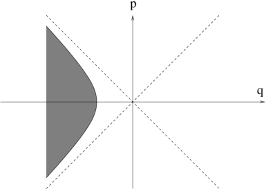
Figure 12: Semi-classical representation of the vacuum state in the matrix model.

If $\Psi(q,t)$ denotes the second quantized fermion field describing the above non-relativistic system, then the massless ‘tachyon’ field in the closed string sector is identified with the scalar field obtained by the bosonization of the fermion field $\Psi$[101, 491, 208]. The precise correspondence goes as follows. The classical equation of motion satisfied by the field $\Psi(q,x^{0})$ has the form:

$$i{\partial\Psi\over\partial x^{0}}+{1\over 2}\,{\partial^{2}\Psi\over\partial q^{2}}+{1\over 2}\,q^{2}\Psi-{1\over g_{s}}\,\Psi=0\,.$$ (11.57)

We now define the ‘time of flight’ variable $\tau$ that is related to $q$ via the relation:

$$q=-\sqrt{2\over g_{s}}\,\cosh\tau\,,\qquad\tau<0\,.$$ (11.58)

$|\tau|$ measures the time taken by a zero energy classical particle moving under the Hamiltonian (11.55) to travel from $-\sqrt{2\over g_{s}}$ to $q$. We also define

$$v(q)=-\sqrt{q^{2}-{2\over g_{s}}}=\sqrt{2\over g_{s}}\,\sinh\tau\,.$$ (11.59)

$|v(q)|$ gives the magnitude of the classical velocity of a zero energy particle when it is at position $q$. Using these variables, it is easy to see that for large negative $\tau$ the solution to eq.(11.57) takes the form:

$$\Psi(q,x^{0})={1\over\sqrt{-2v(q)}}\,\left[e^{-i\int^{q}v(q^{\prime})dq^{\prime}+i\pi/4}\,\Psi_{R}(\tau,x^{0})+e^{i\int^{q}v(q^{\prime})dq^{\prime}-i\pi/4}\,\Psi_{L}(\tau,x^{0})\right]\,,$$ (11.60)

where $\Psi_{L}$ and $\Psi_{R}$ satisfy the field equations:

$$(\partial_{0}-\partial_{\tau})\,\Psi_{L}(\tau,x^{0})=0,\qquad(\partial_{0}+\partial_{\tau})\,\Psi_{R}(\tau,x^{0})=0\,.$$ (11.61)

Thus at large negative $\tau$ we can regard the system as a theory of a pair of chiral fermions, one left-moving and the other right-moving. Of course there is an effective boundary condition at $\tau=0$ which relates the two fermion fields, since a particle coming in from $\tau=-\infty$ will be reflected from $\tau=0$ and will go back to $\tau=-\infty$. Since $\tau$ ranges from 0 to $-\infty$, we can interprete $\Psi_{R}$ as the incoming wave and $\Psi_{L}$ as the outgoing wave.

Eq.(11.61) shows that $\Psi_{L}$ and $\Psi_{R}$ represent a pair of relativistic fermions for large negative $\tau$. Thus we can bosonize them into a pair of chiral bosons $\chi_{L}$ and $\chi_{R}$. This pair of chiral bosons may in turn be combined into a full scalar field $\chi(\tau,x^{0})$ which satisfy the free field equation of motion for large negative $\tau$ and satisfies an appropriate boundary condition at $\tau=0$. If $\chi$ is defined with the standard normalization, then for large negative $\tau$ a single right moving fermion is represented by the configuration[93, 353]

$$\chi=\sqrt{\pi}\,H(x^{0}-\tau)\,,$$ (11.62)

and a single left-moving fermion is represented by the configuration

$$\chi=\sqrt{\pi}\,H(x^{0}+\tau)\,,$$ (11.63)

where $H(u)$ denotes the step function defined in (11.44).

The field $\chi(\tau,x^{0})$ is related to the tachyon field $\phi(\varphi,x^{0})$ in the continuum description of string theory by a non-local field redefinition[381]. In momentum space the relation is[432, 290, 123, 396]:

$$\widetilde{\chi}(P,E)={\Gamma(iP)\over\Gamma(-iP)}\,\widetilde{\phi}(P,E)\,.$$ (11.64)

Using (11.16) this gives

$$\widetilde{\chi}(P,E)=\psi(P,E)\,,$$ (11.65)

and hence

$$\chi(\tau,x^{0})=\psi(\tau,x^{0})\,.$$ (11.66)

Using (11.45) and (11.66) we see that the background $\chi$ associated with a rolling tachyon solution is given by

$$\chi(\tau,x^{0})=\sqrt{\pi}\,H(x^{0}+\tau+\ln\sin(\pi\widetilde{\lambda}))$$ (11.67)

for large positive $x^{0}$ and large negative $\varphi$. According to (11.63) this precisely represents a single left-moving (outgoing) fermion. This shows that the non-BPS D0-brane of the two dimensional string theory can be identified as a state of the matrix theory where a single fermion is excited from the fermi level to some energy $>0$[363, 364, 292].

The classical configuration (11.67) has infinite energy in the scalar field theory. In the fermionic description this infinite energy is the result of infinite quantum uncertainty in momentum for a sharply localized particle in the position space. Thus the classical limit of the fermionic theory does not have this infinite energy. This is the origin of the apparent discrepancy between the classical open string calculation of the D0-brane energy which gives a finite answer (11.38) and the classical closed string calculation which gives infinite answer[292]. We hope that a similar interpretation can be given for the infinite energy carried by the closed string configuration produced by a ‘decaying’ D-brane in the critical string theory as discussed in section 10.1.

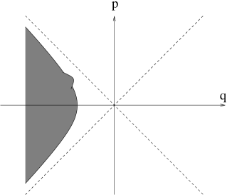
Figure 13: Semiclassical representation of a closed string tachyon field configuration in the matrix model.

Note that strictly speaking the above analysis, leading to the identification of the D0-brane with the single fermion excitation, holds only close to the fermi level, i.e. near $\widetilde{\lambda}=1/2$. From the continuum viewpoint this requirement comes from the fact that the effect of $|{\cal B}_{2}\rangle$ which has not been taken into account so far, can be ignored only in the $\widetilde{\lambda}\to{1\over 2}$ limit. From the matrix model side this requirement comes due to the fact that the bosonization of the fermion system in terms of a single scalar field holds only for excitations close to the fermi level[425]. Nevertheless it is natural to assume that the correspondence between a D0-brane and single fermion excitations continues to hold for general $\widetilde{\lambda}$. In this description the D0-brane with the tachyon field sitting at the maximum of the potential corresponds to the configuration $p=0$, $q=0$. The mass of the D0-brane is then given by $h(0,0)=1/g_{s}$. On the other hand the rolling tachyon solution in open string theory, characterized by the parameter $\widetilde{\lambda}$, corresponds to the phase space trajectory

$$q=-\sqrt{2\over g_{s}}\,\sin(\pi\widetilde{\lambda})\,\cosh x^{0},\qquad p=-\sqrt{2\over g_{s}}\,\sin(\pi\widetilde{\lambda})\,\sinh x^{0}$$ (11.68)

as can be seen by comparing the energies of the rolling tachyon system (eq.(11.38)) and the system described by the Hamiltonian (11.55). The $\widetilde{\lambda}\to{1\over 2}$ limit corresponds to a trajectory at the fermi level.

We can now use this correspondence to find an interpretation for the exponentially growing component $|\Psi^{(2)}_{c}\rangle$ of the string field produced by $|{\cal B}_{2}\rangle$. Since $|{\cal B}_{2}\rangle$ contains information about the conserved charges, what we need is the identification of these charges in the matrix model. An infinite set of conserved charges of this type do indeed exist in the quantum theory of a single fermion described by (11.55). These are of the form[491, 381, 375, 537, 102, 538, 31, 291, 264, 122]:

$$e^{(k-l)x^{0}}(p+q)^{l}(q-p)^{k}\,,$$ (11.69)

where $k$ and $l$ are integers. Requiring that the canonical transformations generated by these charges preserve the fermi level $h(q,p)=0$ [537] gives us a more restricted class of charges:

$$h(q,p)\,e^{(k-l)x^{0}}(p+q)^{l}(q-p)^{k}=\left({1\over 2}(p^{2}-q^{2})+{1\over g_{s}}\right)\,e^{(k-l)x^{0}}(p+q)^{l}(q-p)^{k}\,.$$ (11.70)

Thus it is natural to identify these with linear combinations of the charges $e^{2mx^{0}}g_{j,m}(x^{0})$ in the continuum theory. In order to find the precise relation between these charges we can first compare the explicit $x^{0}$ dependence of the two sets of charges. This gives:

$$k-l=2m\,.$$ (11.71)

Thus the conserved charge $e^{2mx^{0}}g_{j,m}(x^{0})$ should correspond to some specific linear combination of the charges given in (11.70) subject to the condition (11.71):

$$g_{j,m}(x^{0})\leftrightarrow g_{s}\,\left({1\over 2}(p^{2}-q^{2})+{1\over g_{s}}\right)\,\sum_{k\in Z\atop k\geq 0,2m}\,\left({2\over g_{s}}\right)^{m-k}\,a^{(j,m)}_{k}\,(q-p)^{k}(q+p)^{k-2m}\,.$$ (11.72)

Here $a^{(j,m)}_{k}$ are constants and the various $g_{s}$ dependent normalization factors have been introduced for later convenience. In order to find the precise form of the coefficients $a_{k}^{(j,m)}$ we compare the $\widetilde{\lambda}$ dependence of the two sides for the classical trajectory (11.68). Since for this trajectory

$$q\pm p=-\sqrt{2\over g_{s}}\,\sin(\pi\widetilde{\lambda})\,e^{\pm x^{0}}\,,$$ (11.73)

and $g_{j,m}(x^{0})=e^{-2mx^{0}}\,f_{j,m}(\widetilde{\lambda})$, we have:

$$f_{j,m}(\widetilde{\lambda})=(-1)^{2m}\,\left(1-\sin^{2}(\pi\widetilde{\lambda})\right)\,\sum_{k\in Z\atop k\geq 0,2m}\,a^{(j,m)}_{k}\,\sin^{2k-2m}(\pi\widetilde{\lambda})\,.$$ (11.74)

Thus by expanding $f_{j,m}(\widetilde{\lambda})$ given in (7.35) in powers of $\sin(\pi\widetilde{\lambda})$ we can determine the coefficients $a^{(j,m)}_{k}$. One consistency check for this procedure is that on the right hand side the expansion in powers of $\sin(\pi\widetilde{\lambda})$ starts at order $\sin^{2|m|}(\pi\widetilde{\lambda})$. It can be verified that the expansion of $f_{j,m}(\widetilde{\lambda})$ also starts at the same order. The other consistency check is that the right hand side of (11.74) vanishes at $\widetilde{\lambda}={1\over 2}$, which is also the case for $f_{j,m}(\widetilde{\lambda})$. One can also show [488, 490] that these relations are invertible, i.e. the charges $h(q,p)\,(q-p)^{2m+l}\,(q+p)^{l}$ may be expressed as linear combinations of $g_{j,m}(x^{0})$ for $|m|+1\leq j\leq m+l+1$. This shows that the conserved charges $g_{j,m}(x^{0})$ in the continuum theory contains information about the complete set of symmetry generators in the matrix model description of the D0-brane.

Given that the boundary state $|{\cal B}_{2}\rangle$ carries information about the conserved charges, the closed string field produced by $|{\cal B}_{2}\rangle$ must also carry the same information. These can be regarded as the analog of the long range electric or gravitational field produced by a particle carrying charge or mass. Ref.[490] gives a systematic procedure for relating the conserved charges to the asymptotic closed string field configuration at large negative $\varphi$ associated with the discrete states.

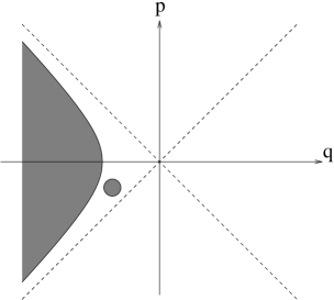
Figure 14: Semi-classical representation of a state of the D0-brane in the matrix model.

In the context we note that by carefully examining the bosonization rules for a fermion moving under the influence of inverted harmonic oscillator potential, ref.[103] has argued that in order to describe the motion of a single fermion in the language of closed string theory, we need to switch on infinite number of closed string fields besides the tachyon. The essential point is that whereas a closed string tachyon mode describes a deformation of the fermi surface of the form shown in Fig.13, the D0-brane is represented by a blob in the phase space disconnected from the Fermi surface as in Fig.14. We believe that the presence of the additional closed string background (11.54) associated with the discrete states is a reflection of this effect. As a consistency check we note that at $\widetilde{\lambda}=1/2$ the additional background (11.54) vanish. This is expected to be true in the matrix model description as well since in this limit the blob merges with the fermi sea[103].

To summarize, we see that a D0-brane in the continuum two dimensional string theory is described in the matrix model as a single fermion excited from the fermi level to some positive energy state. This provides a satisfactory picture of the D0-brane. But this correspondence also raises a puzzle. In the matrix model there is another natural class of states, namely the single hole states, which correspond to a single fermion exited from some state below the fermi level to the fermi level. One might expect that just like the single fermion states, the single hole states should also have some natural description in the continuum string theory. So far however we do not have a completely satisfactory description of these states in the matrix model. Some proposal for what these states might correspond to have been made in [133, 171]. According to this proposal the boundary state describing a hole is obtained by analytically continuing the boundary state of a rolling tachyon configuration to $\widetilde{\lambda}={1\over 2}+i\alpha$ for a real parameter $\alpha$ and then changing the overall sign of the boundary state. Although this produces the right values for the conserved charges carried by the hole, neither the space-time nor the world-sheet interpretation of these states is very clear[490]. An alternative suggestion, according to which the hole states correspond to ordinary D0-branes moving under the influence of the linear dilaton background has been put forward in [490]. We hope that this question will be resolved in the near future.

11.6 D0-brane decay in type 0B string theory

Although two dimensional bosonic string theory provides a useful arena for studying the decay of D0-branes beyond leading order in perturbation theory, it suffers from one problem; the theory, although well defined to all orders in string perturbation theory, is not non-perturbatively stable. In the continuum description of the D0-brane this is due to the fact that the tachyon potential on the D0-brane, while having a local minimum at some positive value of the tachyon field, is expected to be unbounded from below on the negative side. The problem associated with this can be seen for example in the analysis of the time dependent solutions where the tachyon rolling on the wrong side of the potential causes a divergence in the dilaton charge at a finite time. In the matrix model description the instability is related to the fact that the fermi level is filled on only one side of the potential leaving the other side empty. Such a vacuum, while perturbatively stable, is non-perturbatively unstable. Hence while the matrix model - two dimensional string theory correspondence illustrates many aspects of D0-brane decay in perturbation theory, it does not allow us to go beyond perturbation theory.

On the matrix model side there is an easy way to solve the problem, – we just fill the fermi level on both sides. This will have the feature that the spectrum of closed strings, which represent excitations around the fermi level, will be doubled since now we can excite fermion hole pairs on either side of the potential. In particular bosonizing the fermion field on the two sides of the potential we should either find two different asymptotic regions with a massless scalar field living in each of these regions, or find one asymptotic region with two massless scalar fields living in this region. This is clearly not the two dimensional bosonic string theory that we have discussed so far which has only one asymptotic region ($\varphi\to-\infty$) with one massless scalar field. Is there some other two dimensional string theory that corresponds to this particular matrix model? It turns out that the answer is yes: it is two dimensional type 0B string theory[510, 133, 515].

The local world sheet dynamics of type 0 string theories is identical to that of type II string theories, i.e. it has both left and right moving world-sheet supersymmetry. Thus the critical dimension for this theory is 10, which is equivalent to saying the matter part of the theory must have $\hat{c}=10$. The difference with type II string theories comes in the GSO projection rules. Whereas the type II string theories have separate GSO projection on the left and the right sector, type 0 theories have one combined GSO projection[430]. Due to modular invariance this then requires that the theory contains NS-NS and RR sector states, but no NS-R or R-NS sector states. In other words, the closed string sector does not contain fermions! As in the case of type II string theories, we can construct two types of type 0 string theories, 0A and 0B, which differ from each other in the sign of the GSO projection operator in the RR sector.

As in the case of bosonic string theory where we can construct a two dimensional string theory by replacing 25 of the scalar fields by a Liouville theory with total central charge 25, we can also construct two dimensional type 0A and 0B string theories by replacing nine of the space-like world-sheet superfields by a super-Liouville theory. This theory contains a single superfield with exponential potential and background charge such that it describes a super-conformal field theory with $\hat{c}=9$. This gives rise to the so called two dimensional type 0 string theories. In particular type 0B theory has two independent massless scalar fields in the closed string spectrum, one coming from the RR sector and the other coming from the NS-NS sector. Thus it is natural to conjecture that this two dimensional string theory is equivalent to the matrix model described earlier, with the two scalars being identified with appropriate linear combinations of the excitations on the fermi level on two sides of the potential[510, 133]. This is verified by computing the S-matrix involving these fields in the type 0B theory and comparing them with the predictions of the matrix model[123, 120]. The only subtle point to keep in mind is that the matrix model Hamiltonian (11.55) seems to correspond to type 0B theory with $\alpha^{\prime}=1/2$ rather than $\alpha^{\prime}=1$. We shall work in this unit in the rest of this section.

It turns out that the type 0B string theory has an unstable D0-brane that corresponds to Dirichlet boundary condition on the Liouville coordinate, and the usual Neumann boundary condition on the time coordinate. The open string spectrum on this brane has a tachyonic mode. In the $\alpha^{\prime}=1$ unit the tachyon has mass${}^{2}=-{1\over 2}$ as in the case of unstable D-branes of superstring theory, but in the $\alpha^{\prime}={1\over 2}$ unit that we are using the tachyon has mass${}^{2}=-1$. This agrees with the tachyon mass² obtained by quantizing the inverted harmonic oscillator Hamiltonian (11.55) around $q=0$. We can also construct the rolling tachyon solution by switching on tachyon background proportional to $\cosh x^{0}$ or $\sinh x^{0}$. The world-sheet analysis is identical to that in the case of unstable D-branes in superstring theory except for the scaling of $\alpha^{\prime}$. In particular we can construct the boundary state describing this D0-brane following the procedure discussed earlier and use this to study closed string radiation from the D0-brane. The result gives a kink configuration of the type given in eq.(11.67) showing that the D0-brane is naturally identified with single fermion excitations in the theory[510, 133].

Thus we see that we now have an example of a completely consistent two dimensional string theory and its matrix model description. This allows us to study aspects of D0-brane dynamics in this theory not only to all orders in perturbation theory but also non-perturbatively. We hope that this can be used to derive useful insight into the dynamics of unstable D-branes in critical string theories, particularly in the context of the open string completeness conjecture to be discussed in section 12.

Various other aspects of D0-brane decay in two dimensional string theory have been discussed in [217, 106, 12, 266].

12 Open String Completeness Conjecture

The straightforward analysis of closed string emission from unstable D0-branes (or D$p$-branes wrapped on $T^{p}$) tell us that all the energy of the D0-brane is radiated away into closed strings, both in the critical string theory and in the two dimensional string theory. Naively this would suggest that the backreaction due to the closed string emission process invalidates the classical open string results. However we shall argue in this section that results obtained from the tree level open string theory actually give dual description of the closed string emission process.

12.1 Open string completeness in the critical string theory

We begin our discussion by analyzing the results for D-brane decay in critical string theory. In order to illustrate the proposed duality between open string and closed string description, let us compare the properties of the emitted closed strings from an unstable D$p$-brane wrapped on $T^{p}$ with those infered from the tree level open string analysis[170, 483, 275, 484]. First of all, tree level open string analysis tells us that the final system has:

$$Q/T_{00}=0\,,$$ (12.1)

where $Q$ and $T_{00}$ denote the dilaton charge density and energy density of the system respectively. On the other hand by examining the closed string world-sheet action in the background string metric $G_{\mu\nu}$, the anti-symmetric tensor field $B_{\mu\nu}$ and the dilaton $\Phi_{D}$ at zero momentum,

$$S_{world-sheet}={1\over 2\pi}\,\int d^{2}z(G_{\mu\nu}(X)+B_{\mu\nu}(X))\partial_{z}X^{\mu}\partial_{\bar{z}}X^{\nu}\,,$$ (12.2)

we see that the closed string world-sheet does not couple to the zero momentum dilaton. This shows the final state closed strings carry zero total dilaton charge. Hence the dilaton charge of the final state closed strings agrees with that computed in the open string description.

Next we note that the tree level open string analysis tells us that the final system has:

$$p/T_{00}=0\,,$$ (12.3)

where $p$ denotes the pressure of the system. On the other hand, closed string analysis tells us that the final closed strings have mass $m$ of order $1/g_{s}$, momentum $k_{\perp}$ transverse to the D-brane of order $1/\sqrt{g_{s}}$ and winding $w_{\parallel}$ tangential to the D-brane of order $1/\sqrt{g_{s}}$. For such a system the ratio of transverse pressure to the energy density is of order $(k_{\perp}/m)^{2}\sim g_{s}$ and the ratio of tangential pressure to the energy density is of order $-(w_{\parallel}/m)^{2}\sim-g_{s}$. Since both these ratios vanish in the $g_{s}\to 0$ limit, we again see that the pressure of the final state closed strings match the result computed in the open string description.

Such agreements between open and closed string results also hold for more general cases, e.g. in the decay of unstable branes in the presence of electric field. Consider, for example, the decay of a D$p$-brane along $x^{1},\ldots x^{p}$ plane, with an electric field $e$ along the $x^{1}$ axis. In this case the final state is characterized by its energy-momentum tensor $T_{\mu\nu}$, source $S_{\mu\nu}$ for anti-symmetric tensor field $B_{\mu\nu}$ and the dilaton charge density $Q$. One can show that in the $x^{0}\to\infty$ limit[391, 448, 449]:

$$T^{00}=|\Pi|\,e^{-1}\,\delta(\vec{x}_{\perp})\,,\quad T^{11}=-|\Pi|\,e\,\delta(\vec{x}_{\perp})\,,\quad S^{01}=\Pi\,\delta(\vec{x}_{\perp})\,,$$ (12.4)

where $\Pi$ is a parameter labelling the solution. All other components of $T_{\mu\nu}$ and $S_{\mu\nu}$, as well as the dilaton charge vanishes in this limit. It can be shown that these tree level open string results again agree exactly with the properties of the final state closed strings into which the D-brane decays[484, 219].

Since in all these cases the tree level open string results for various properties of the final state agree with the properties of the closed strings produced in the decay of the brane, we are led to conjecture that the tree level open string theory provides a description of the rolling tachyon system which is dual to the description in terms of closed string emission[483, 484].^, This is different from the usual open closed duality where one loop open string theory contains information about closed strings. In order to put this conjecture on a firmer footing, one must show that it arises from a more complete conjecture involving full quantum open string theory on an unstable D-brane. The full conjecture, suggested in [485, 487], takes the following form:

There is a quantum open string field theory (OSFT) that describes the full dynamics of an unstable Dp-brane without an explicit coupling to closed strings. Furthermore, Ehrenfest theorem holds in the weakly coupled OSFT; the classical results correctly describe the time evolution of the quantum expectation values.

Since the conjecture in essence says that quantum open string theory is fully capable of describing the complete dynamics of an unstable D-brane, we call this the open string completeness conjecture. Stated this way, this conjecture also embodies the usual perturbative open-closed string duality for a stable D-brane where the open string loop amplitudes contain information about closed string exchange processes. In this case the quantum open string field theory is fully capable of reproducing the open string scattering amplitudes at least to all orders in perturbation theory[192, 156]. For example for this system quantum open string theory gives rise to the cylinder contribution to the string partition function at one loop order. Coupling closed strings to this system as in eqs.(A.4), (A.5) will ensure that by eliminating the closed string fields by their classical equations of motion we get the cylinder amplitude again as in eq.(A.8). This gives a clear indication that including closed strings in open string field theory amounts to double counting.

Note that this open string completeness conjecture does not imply that the quantum open string theory on a given system of unstable (or stable) D-branes gives a complete description of the full string theory. It only states that this open string field theory describes a quantum mechanically consistent subsector of the full string theory, and is fully capable of describing the quantum dynamics of the D-brane. One of the consequences of this correspondence is that the notion of naturalness of a solution may differ dramatically in the open and the closed string description. A solution describing the decay of a single (or a few) unstable D-branes may look highly contrived in the closed string description, since a generic deformation of this background in closed string theory may not be describable by the dynamics of a single D-brane, and may require a large (or even infinite) number of D-branes for its description in open string theory.

In our discussion of the properties of the closed string states emitted from a ‘decaying’ D-brane we have so far only included closed string radiation produced by the $|{\cal B}_{1}\rangle$ component of the boundary state. Hence our analysis is valid only in the $\widetilde{\lambda}\to{1\over 2}$ limit when the closed string background produced by $|{\cal B}_{2}\rangle$ vanishes. As we have seen in section 10.2, for $\widetilde{\lambda}\neq{1\over 2}$ the closed string fields produced by the $|{\cal B}_{2}\rangle$ component of the boundary state grow exponentially with time. Naively, this exponential growth of the closed string field configurations again indicates the breakdown of classical open string description at late time. However in the spirit of the open string completeness conjecture proposed here it is more natural to seek an alternative interpretation. What this may be indicating is an inadequacy of the weakly coupled closed string description rather than an inadequacy of the open string description. As an analogy we can cite the example of closed string field configurations produced by static stable D-branes. Often the field configuration is singular near the core of the brane. However we do not take this as an indication of the breakdown of the open string description. Instead it is a reflection of the inadequacy of the closed string description.

While in critical string theory the open string completeness remains a conjecture, we shall see in the next subsection that this is bourne out quite clearly in the two dimensional string theory.

12.2 Open string completeness in two dimensional string theory

The analysis of section 11.3 shows that a rolling tachyon configuration on a D0-brane in two dimensional string theory produces an infinitely sharp kink of the closed string tachyon field. Since this carries infinite energy, we might naively conclude that all the energy of the D0-brane is converted to closed string radiation and hence the results of tree level open string analysis cannot be trusted. The analysis of section 11.4 shows that for $\widetilde{\lambda}\neq{1\over 2}$ the closed string field configuration produced by the $|{\cal B}_{2}\rangle$ component of the boundary state grows exponentially with time. This is again a potential source for large backreaction on the tree level open string results.

On the other hand we have seen in section 11.5 that a D0-brane in two dimensional string theory can be identified in the matrix model description as a single fermion excitation from the fermi level to some energy level above 0. Since the fermions are non-interacting, the states with a single excited fermion do not mix with any other states in the theory (say with states where two or more fermions are excited above the fermi level or hole states where a fermion is excited from below the fermi level to the fermi level). As a result, the quantum states of a D0-brane are in one to one correspondence with the quantum states of the single particle Hamiltonian

$$h(q,p)={1\over 2}(p^{2}-q^{2})+{1\over g_{s}}\,,$$ (12.5)

with one additional constraint, – the spectrum is cut off sharply for energy below zero due to Pauli exclusion principle. Since by definition quantum open string field theory on a D-brane is a field theory that describes the dynamics of that D-brane, we see that in the matrix model description the ‘quantum open string field theory’ for a single D0-brane is described by the inverted harmonic oscillator hamiltonian (12.5) with all the negative energy states removed by hand[485]. The classical limit of this quantum Hamiltonian is described by the classical Hamiltonian (12.5), with a sharp cut-off on the phase space variables:

$${1\over 2}(p^{2}-q^{2})+{1\over g_{s}}\geq 0\,.$$ (12.6)

This is the matrix model description of ‘classical open string field theory’ describing the dynamics of a D0-brane.

Clearly the quantum system described above provides us with a complete description of the dynamics of a single D0-brane. In particular there is no need to couple this system explicitly to closed strings, although closed strings could provide an alternative description of the D0-brane as a kink solution in the closed string ‘tachyon’ field (as given in (11.67)). This is in accordance with the open string completeness conjecture discussed in section 12.1. From this it is clear that it is a wrong notion to think in terms of backreaction of closed string fields on the open string dynamics. Instead we should regard the closed string background produced by the D-brane as a way of characterizing the open string background (although the open string theory itself is sufficient for this purpose). For example, in the present context, we can think of the closed string tachyon field $\chi(\tau,x^{0})$ at late time as the expectation value of the operator

$$\hat{\chi}(\tau,x^{0})\equiv\sqrt{\pi}\,H\left(-\hat{q}(x^{0})-\sqrt{2\over g_{s}}\cosh\tau\right)\,$$ (12.7)

in the quantum open string theory on a single D0-brane, as described by (12.5), (12.6). In (12.7) $\hat{q}$ denotes the position operator in the quantum open string theory. When we calculate the expectation value of $\hat{\chi}$ in the quantum state whose classical limit is described by the trajectory (11.68), we can replace $\widehat{q}$ by its classical value $q=-\sqrt{2\over g_{s}}\sin(\pi\widetilde{\lambda})\cosh(x^{0})$. This gives

$$\langle\hat{\chi}(\tau,x^{0})\rangle=\sqrt{\pi}\,H\left(\sqrt{2\over g_{s}}\,\sin(\pi\widetilde{\lambda})\,\cosh(x^{0})-\sqrt{2\over g_{s}}\cosh\tau\right)\simeq\sqrt{\pi}\,H(x^{0}+\tau+\ln\sin(\pi\widetilde{\lambda}))\,,$$ (12.8)

for large $x^{0}$ and negative $\tau$. This reproduces (11.67).

In a similar spirit we note that while the naive analysis of the closed string field configuration produced by the $|{\cal B}_{2}\rangle$ component of the boundary state indicates that the exponentially growing closed string fields produce large backreaction and hence invalidates the analysis based on open string theory, the results of section 11.5 clearly point to a different direction. According to these results the exponentially growing terms in $|{\cal B}_{2}\rangle$ are simply consequences of the conserved charges a D0-brane carries, which in turn may be calculated completely within the framework of the open string (field) theory. Thus these exponentially growing terms do not in any way point to an inadequacy of the open string description of D0-brane dynamics.

Various other aspects of the open string completeness conjecture in the context of two dimensional string theory have been discussed in [112, 11, 352].

12.3 Generalized holographic principle

We have seen in the previous two subsections that the analysis of unstable D-brane ‘decay’ in critical string theory as well as in the two dimensional string theory points to the conjecture that the quantum open string field theory on a given D-brane describes complete quantum dynamics of the D-brane. However generically a given D-brane system does not have the ability to describe an arbitrary state in string theory, – it carries only partial information about the full theory. This conjecture makes it clear that open string field theory on a single or a finite number of D-branes must be encoding information about the full string theory in a highly non-local manner. For example when a D-brane ‘decays’ into closed strings we expect that at least some of the closed strings will eventually disperse to infinity. The open string field theory, defined in terms of variables localized near the original D-brane, must be able to describe the final closed string state produced in the decay, although it may not be able to describe states of the individual closed strings into which the D-brane decays. The situation can be described by drawing analogy to a hologram. If we regard the full string theory as the complete image produced by a hologram, then a system of finite number of D-branes can be regarded as a part of the hologram. This encodes partial information about the full image. However the information contained in any given piece of the hologram does not correspond to a given part of the complete image; instead it has partial information about all parts of the image. Thus the open string completeness conjecture proposed here can be thought of as a generalization of the holographic principle[211, 503, 347, 211, 542, 504]. As in these papers in our proposal the relation between the open and closed string description is non-local, but the space in which the open string degress of freedom live is not necessarily the boundary of the space in which the closed string degrees of freedom live.

Acknowledgement: I would like to thank my collaborators N. Berkovits, D. Gaiotto, D. Ghoshal, J. Majumder, N. Moeller, P. Mukhopadhyay, L. Rastelli and B. Zwiebach for collaboration on various aspects of open string tachyon dynamics.

Appendix A Energy-Momentum Tensor from Boundary State

As discussed in section 3.3, given a boundary CFT describing a D-brane system, we define the corresponding boundary state $|{\cal B}\rangle$ such that given any closed string state $|V\rangle$ and the associated vertex operator $V$,

$$\langle{\cal B}|V\rangle\propto\langle V(0)\rangle_{D}\,,$$ (A.1)

where $\langle V(0)\rangle_{D}$ is the one point function of $V$ inserted at the centre of a unit disk $D$, the boundary condition / interaction on $\partial D$ being the one associated with the particular boundary CFT under consideration. From this definition it is clear that the boundary state contains information about what kind of source for the closed string states is produced by the D-brane system under consideration. In this appendix we shall make this more precise by working with (linearized) closed string field theory[553].

For simplicity we shall focus on the bosonic string theory. The closed string field corresponds to a state $|\Psi_{c}\rangle$ of ghost number 2 in the Hilbert space of matter ghost conformal field theory in the full complex plane, satisfying the constraint[553]

$$b_{0}^{-}|\Psi_{c}\rangle=0\,,\qquad L_{0}^{-}|\Psi_{c}\rangle=0\,,$$ (A.2)

where

$$c_{0}^{\pm}=(c_{0}\pm\bar{c}_{0}),\qquad b_{0}^{\pm}=(b_{0}\pm\bar{b}_{0})\,,\qquad L_{0}^{\pm}=(L_{0}\pm\bar{L}_{0})\,.$$ (A.3)

$c_{n}$, $\bar{c}_{n}$, $b_{n}$, $\bar{b}_{n}$ are the usual ghost oscillators and $L_{n}$, $\bar{L}_{n}$ are the total Virasoro generators. The quadratic part of the closed string field theory action can be taken to be:

$$-{1\over Kg_{s}^{2}}\langle\Psi_{c}|c_{0}^{-}(Q_{B}+\bar{Q}_{B})|\Psi_{c}\rangle\,,$$ (A.4)

where $Q_{B}$ and $\bar{Q}_{B}$ are the holomorphic and anti-holomorphic components of the BRST charge, $K$ is a normalization constant to be determined in eq.(A.8), and $g_{s}$ is the appropriately normalized closed string coupling constant so that (2.1) holds. In the presence of the D-brane we need to add an extra source term to the action:

$$\langle\Psi_{c}|c_{0}^{-}|{\cal B}\rangle\,.$$ (A.5)

The equation of motion of $|\Psi_{c}\rangle$ is then

$$2\,(Q_{B}+\bar{Q}_{B})\,|\Psi_{c}\rangle=K\,g_{s}^{2}\,|{\cal B}\rangle\,.$$ (A.6)

Clearly by a rescaling of $|\Psi_{c}\rangle$ by $\lambda$ we can change $K$ and $|{\cal B}\rangle$ to $K/\lambda^{2}$ and $\lambda|{\cal B}\rangle$ respectively. However once the normalization of $|{\cal B}\rangle$ is fixed in a convenient manner, the normalization constant $K$ can be determined by requiring that the classical action obtained after eliminating $|\Psi_{c}\rangle$ using its equation of motion (A.6) reproduces the one loop partition function $Z_{open}$ of the open string theory on the D-brane. Choosing the solution of (A.6) to be

$$|\Psi_{c}\rangle={1\over 2}\,K\,g_{s}^{2}\,b_{0}^{+}\,(L_{0}^{+})^{-1}\,|{\cal B}\rangle\,,$$ (A.7)

we get

$$Z_{open}=-{1\over 4}\,K\,g_{s}^{2}\,\langle{\cal B}|b_{0}^{+}\,c_{0}^{-}\,(L_{0}^{+})^{-1}\,|{\cal B}\rangle\,.$$ (A.8)

We have chosen a convenient normalization of $|{\cal B}\rangle$ in eq.(3.35). This determines $K$ from eq.(A.8). Since $Z_{open}$ is independent of $g_{s}$, and $|{\cal B}\rangle$ is inversely proportional to $g_{s}$ due to the ${\cal T}_{p}$ factor in (3.35), we see that $K$ is a purely numerical constant.

Eqs.(A.5), (A.6) clearly shows that $|{\cal B}\rangle$ represents the source for the closed string fields in the presence of a D-brane. We shall now make it more explicit by expanding $|\Psi_{c}\rangle$ and $|{\cal B}\rangle$ in the oscillator basis. The expansion of $|\Psi_{c}\rangle$ in the oscillator basis of closed string states has, as coefficients, various closed string fields. For example the first few terms in the expansion are:

$$\displaystyle|\Psi_{c}\rangle = \int{d^{26}k\over(2\pi)^{26}}\,\bigg{[}\widetilde{T}(k)c_{1}\bar{c}_{1}+\left(\widetilde{h}_{\mu\nu}(k)+\widetilde{b}_{\mu\nu}(k)\right)\alpha^{\mu}_{-1}\bar{\alpha}^{\nu}_{-1}c_{1}\bar{c}_{1}$$ (A.9)

$$+\left(\widetilde{\phi}(k)+{1\over 2}\eta^{\mu\nu}\widetilde{h}_{\mu\nu}(k)\right)(c_{1}c_{-1}-\bar{c}_{1}\bar{c}_{-1})+\ldots\bigg{]}|k\rangle$$

where $\alpha^{\mu}_{n}$, $\bar{\alpha}^{\mu}_{n}$ are the usual oscillators associated with the $X^{\mu}$ fields. In this expansion $\widetilde{T}(k)$ has the interpretation of the Fourier transform of the closed string tachyon field, $\widetilde{h}_{\mu\nu}=\widetilde{h}_{\nu\mu}$ and $\widetilde{\phi}(k)$ are Fourier transforms of the graviton (associated with the string metric) and the dilaton fields respectively, $\widetilde{b}_{\mu\nu}=-\widetilde{b}_{\nu\mu}$ is the Fourier transform of the anti-symmetric tensor field etc. On the other hand the boundary state $|{\cal B}\rangle$ has an expansion of the form:

$$\displaystyle|{\cal B}\rangle = \int{d^{26}k\over(2\pi)^{26}}\left[\widetilde{F}(k)+\left(\widetilde{A}_{\mu\nu}(k)+\widetilde{C}_{\mu\nu}(k)\right)\alpha^{\mu}_{-1}\bar{\alpha}^{\nu}_{-1}+\widetilde{B}(k)(b_{-1}\bar{c}_{-1}+\bar{b}_{-1}c_{-1})+\ldots\right]$$ (A.10)

$$\qquad\qquad\qquad\qquad\qquad\qquad(c_{0}+\bar{c}_{0})c_{1}\bar{c}_{1}|k\rangle\,,$$

where $\widetilde{F}$, $\widetilde{A}_{\mu\nu}=\widetilde{A}_{\nu\mu}$, $\widetilde{C}_{\mu\nu}=-\widetilde{C}_{\nu\mu}$, $\widetilde{B}$ etc. are fixed functions which can be read out of the boundary state $|{\cal B}\rangle$. Substituting (A.9) and (A.10) into eq.(A.5) we get terms in the action proportional to

$$\int\,{d^{26}k\over(2\pi)^{26}}\,\left[\widetilde{h}_{\mu\nu}(-k)\left(\widetilde{A}^{\mu\nu}(k)+\widetilde{B}(k)\,\eta^{\mu\nu}\right)+2\widetilde{\phi}(-k)\,\widetilde{B}(k)+\cdots\right]\,,$$ (A.11)

where $\cdots$ denote source terms for other fields. Since the Fourier transform $\widetilde{T}^{\mu\nu}$ of the energy momentum tensor couples to $\widetilde{h}_{\mu\nu}$, we see that $\widetilde{T}_{\mu\nu}$ is proportional to $\widetilde{A}_{\mu\nu}(k)+\eta_{\mu\nu}\,\widetilde{B}(k)$.

We can also use an alternative but equivalent method for expressing the energy momentum tensor $T_{\mu\nu}$ in terms of $A_{\mu\nu}$ and $B$ by using the conservation law of $T_{\mu\nu}$. (A.6) together with nilpotence of $(Q_{B}+\bar{Q}_{B})$ gives:

$$(Q_{B}+\bar{Q}_{B})|{\cal B}\rangle=0\,.$$ (A.12)

Substituting the expansion (A.10) into this equation gives, besides other equations,

$$k^{\nu}\widetilde{A}_{\mu\nu}(k)+k_{\mu}\widetilde{B}(k)=0\,.$$ (A.13)

If $A_{\mu\nu}(x)$ and $B(x)$ denote the Fourier transforms of $\widetilde{A}_{\mu\nu}$ and $\widetilde{B}$ respectively,

$$A_{\mu\nu}(x)=\int{d^{26}k\over(2\pi)^{26}}\,e^{ik\cdot x}\widetilde{A}_{\mu\nu}(k)\,,\qquad B(x)=\int{d^{26}k\over(2\pi)^{26}}\,e^{ik\cdot x}\widetilde{B}(k)\,,$$ (A.14)

then (A.13) gives us:

$$\partial^{\nu}(A_{\mu\nu}(x)+\eta_{\mu\nu}B(x))=0\,.$$ (A.15)

This shows that we should identify the conserved energy-momentum tensor as

$$T_{\mu\nu}(x)\propto(A_{\mu\nu}(x)+\eta_{\mu\nu}B(x))\,.$$ (A.16)

From (A.11) we also see that the function $\widetilde{B}(k)$ measures the source of the dilaton field $\widetilde{\phi}(k)$. This suggests that in position space we define the source of the dilaton to be

$$Q(x)\propto B(x)\,.$$ (A.17)

Appendix B Computation of the Energy of Closed String Radiation from Unstable D-brane

(10.1) gives the on-shell closed string field configuration produced by the rolling tachyon background. In this appendix we shall compute the energy per unit $p$-volume carried by this background. For this we express $(Q_{B}+\bar{Q}_{B})$, acting on a state carrying momentum $\{k^{\mu}\}$, as

$$Q_{B}+\bar{Q}_{B}=(c_{0}L_{0}+\bar{c}_{0}\bar{L}_{0})+\widehat{Q}_{1}(\vec{k})k^{0}+\widehat{Q}_{2}(\vec{k})\,,$$ (B.1)

where the operators $\widehat{Q}_{1}(\vec{k})$ and $\widehat{Q}_{2}(\vec{k})$ do not have any explicit $k^{0}$ dependence but can depend on the spatial components of the momentum $\vec{k}$. The reason that the right hand side of (B.1) does not contain higher powers of $k^{0}$ is that the $k^{\mu}$ dependence of $(Q_{B}+\bar{Q}_{B})$ comes through the $k^{\mu}$ dependence of the matter Virasoro generators $L^{(m)}_{n}$ and $\bar{L}^{(m)}_{n}$, and for $n\neq 0$ $L^{(m)}_{n}$ and $\bar{L}^{(m)}_{n}$ are linear in $k^{\mu}$. Contribution from the $L_{0}$ and $\bar{L}_{0}$ part of $Q_{B}+\bar{Q}_{B}$, which are quadratic in $k^{\mu}$, has been written separately in the right hand side of (B.1). Let us denote by $\widehat{L}$ the part of $(L_{0}+\bar{L}_{0})$ that involves oscillator contribution and contribution from spatial momenta, so that

$$L_{0}+\bar{L}_{0}=-{1\over 2}(k^{0})^{2}+\widehat{L}\,.$$ (B.2)

We also express a general closed string field configuration $|\Psi_{c}\rangle$ as

$$|\Psi_{c}\rangle=\int{dk^{0}\over 2\pi}\,\widetilde{\psi}_{A}(k^{0})\,|k^{0},A\rangle\,,$$ (B.3)

where the label $A$ runs over discrete oscillator labels as well as continuous spatial momenta. The free closed string field theory action (A.4), expressed in terms of the component fields $\widetilde{\psi}_{A}$, takes the form

$$S=-{1\over Kg_{s}^{2}}\,\int\,{dk^{0}\over 2\pi}\,\widetilde{\psi}_{A}(-k^{0})\,\left[-{1\over 2}(k^{0})^{2}N_{AB}+M_{AB}+k^{0}\,M^{(1)}_{AB}+M^{(2)}_{AB}\right]\widetilde{\psi}_{B}(k^{0})\,,$$ (B.4)

where $N_{AB}$, $M_{AB}$, $M^{(1)}_{AB}$ and $M^{(2)}_{AB}$ are defined through the relations:

$$\displaystyle{1\over 2}\langle k^{0},A|c_{0}^{-}c_{0}^{+}|k^{\prime 0},B\rangle = N_{AB}\,2\pi\,\delta(k^{0}+k^{\prime 0})\,,$$

$${1\over 2}\,\langle k^{0},A|c_{0}^{-}c_{0}^{+}\widehat{L}|k^{\prime 0},B\rangle = M_{AB}\,2\pi\,\delta(k^{0}+k^{\prime 0})\,,$$

$$\langle k^{0},A|c_{0}^{-}\widehat{Q}_{1}|k^{\prime 0},B\rangle = M^{(1)}_{AB}\,2\pi\,\delta(k^{0}+k^{\prime 0})\,,$$

$$\langle k^{0},A|c_{0}^{-}\widehat{Q}_{2}|k^{\prime 0},B\rangle = M^{(2)}_{AB}\,2\pi\,\delta(k^{0}+k^{\prime 0})\,.$$

If we denote by

$$\psi_{A}(x^{0})=\int{dk^{0}\over 2\pi}\,e^{-ik^{0}x^{0}}\,\widetilde{\psi}_{A}(k^{0})\,,$$ (B.6)

then the action (B.4) may be reexpressed as

$$S=\int dx^{0}L\,,$$ (B.7)

where

$$L={1\over Kg_{s}^{2}}\,\left[{1\over 2}\partial_{0}\,\psi_{A}N_{AB}\,\partial_{0}\psi_{B}-i\,M^{(1)}_{AB}\,\psi_{A}\,\partial_{0}\psi_{B}-\left(M_{AB}+M^{(2)}_{AB}\right)\,\psi_{A}\,\psi_{B}\right]\,.$$ (B.8)

From this we can write down an expression for the conserved energy:

$$E=\partial_{0}\psi_{A}{\partial L\over\partial(\partial_{0}\psi_{A})}-L={1\over Kg_{s}^{2}}\,\left[{1\over 2}\partial_{0}\,\psi_{A}N_{AB}\,\partial_{0}\psi_{B}+\left(M_{AB}+M^{(2)}_{AB}\right)\,\psi_{A}\,\psi_{B}\right]\,.$$ (B.9)

We shall now evaluate (B.9) for the on-shell closed string background (10.1). For this we express $|\Psi_{c}^{(1)}\rangle$ given in (10.1) as

$$|\Psi_{c}^{(1)}\rangle=\int{dk^{0}\over 2\pi}\,\sum_{N}\,\int{d^{25-p}k_{\perp}\over(2\pi)^{25-p}}\,\widetilde{\psi}^{(1)}_{N}(k^{0},\vec{k}_{\perp})|N,\vec{k}_{\perp},k^{0}\rangle\,,$$ (B.10)

where

$$|N,\vec{k}_{\perp},k^{0}\rangle=\widehat{A}_{N}\,c_{1}\,\bar{c}_{1}\,|k^{0},\vec{k}_{\parallel}=0,\vec{k}_{\perp}\rangle\,$$ (B.11)

and

$$\displaystyle\widetilde{\psi}_{N}^{(1)}(k^{0},\vec{k}_{\perp}) = 2\,K\,g_{s}^{2}\,{\cal T}_{p}\,{\pi\over\sinh(\pi\omega^{(N)}_{\vec{k}_{\perp}})}\,{1\over 2\omega^{(N)}_{\vec{k}_{\perp}}}$$ (B.12)

$$\left[e^{-i\omega^{(N)}_{\vec{k}_{\perp}}\,\ln\sin(\pi\widetilde{\lambda})}\delta(k^{0}-\omega^{(N)}_{\vec{k}_{\perp}})+e^{i\omega^{(N)}_{\vec{k}_{\perp}}\,\ln\sin(\pi\widetilde{\lambda})}\delta(k^{0}+\omega^{(N)}_{\vec{k}_{\perp}})\right]\,.$$

This gives

$$\displaystyle\psi_{N}^{(1)}(x^{0},\vec{k}_{\perp}) \equiv \int{dk^{0}\over 2\pi}\,e^{-ik^{0}x^{0}}\,\widetilde{\psi}_{N}(k^{0},\vec{k}_{\perp})$$

$$= 2\,K\,g_{s}^{2}\,{\cal T}_{p}\,{\pi\over\sinh(\pi\omega^{(N)}_{\vec{k}_{\perp}})}\,{1\over 2\omega^{(N)}_{\vec{k}_{\perp}}}\,\left[e^{-i\omega^{(N)}_{\vec{k}_{\perp}}\,(x^{0}+\ln\sin(\pi\widetilde{\lambda}))}+e^{i\omega^{(N)}_{\vec{k}_{\perp}}\,(x^{0}+\ln\sin(\pi\widetilde{\lambda}))}\right]\,.$$

Using the definitions (B.3) and (B.6) of $\psi_{A}(x^{0})$, definition (B) of $N_{AB}$, $M_{AB}$, $M^{(1)}_{AB}$ and $M^{(2)}_{AB}$, and eq.(B.9), we can now write down an expression for the total energy associated with the configuration $|\Psi_{c}^{(1)}\rangle$ as:

$$\displaystyle E^{(1)} = {1\over Kg_{s}^{2}}\,\int{d^{25-p}k_{\perp}\over(2\pi)^{25-p}}\,\sum_{N}\Big{[}S_{N}\,\partial_{0}\psi_{N}^{(1)}(x^{0},\vec{k}_{\perp})\,\partial_{0}\psi_{N}^{(1)}(x^{0},-\vec{k}_{\perp})$$ (B.14)

$$\qquad\qquad+R_{N}\,\psi_{N}^{(1)}(x^{0},\vec{k}_{\perp})\,\psi_{N}^{(1)}(x^{0},-\vec{k}_{\perp})\Big{]}\,,$$

where $S_{N}$ and $R_{N}$ are defined through

$${1\over 4}\langle N,\vec{k}_{\perp},k^{0}|c_{0}^{-}c_{0}^{+}|N,\vec{k}_{\perp}^{\prime},k^{\prime 0}\rangle=(2\pi)^{26-p}\,\delta(k^{0}+k^{\prime 0})\,\delta^{(25-p)}(\vec{k}_{\perp}+\vec{k}^{\prime}_{\perp})\,S_{N}\,,$$ (B.15)

$$\langle N,\vec{k}_{\perp},k^{0}|c_{0}^{-}({1\over 2}\,c_{0}^{+}\widehat{L}+\widehat{Q}_{2})|N,\vec{k}_{\perp}^{\prime},k^{\prime 0}\rangle=(2\pi)^{26-p}\,\delta(k^{0}+k^{\prime 0})\,\delta^{(25-p)}(\vec{k}_{\perp}+\vec{k}^{\prime}_{\perp})\,R_{N}\,.$$ (B.16)

From the definition of $|N,\vec{k}_{\perp},k^{0}\rangle$ and $\widehat{Q}_{2}$ it follows that neither of them contains a $c_{0}$ or a $\bar{c}_{0}$ zero mode. As a result the matrix element of $c_{0}^{-}\widehat{Q}_{2}$ appearing in (B.16) vanishes. On the other hand $|N,\vec{k}_{\perp}\rangle$ is an eigenstate of $\widehat{L}$ with eigenvalue $2(N-1)+{1\over 2}\vec{k}_{\perp}^{2}={1\over 2}(\omega^{(N)}_{\vec{k}_{\perp}})^{2}$. Thus comparison of (B.15) and (B.16) gives

$$R_{N}=(\omega^{(N)}_{\vec{k}_{\perp}})^{2}S_{N}\,.$$ (B.17)

Substituting this into (B.14), and using (B) we get

$$E^{(1)}=4\,K\,(g_{s}{\cal T}_{p})^{2}\,\sum_{N}\,\int{d^{25-p}k_{\perp}\over(2\pi)^{25-p}}\,S_{N}\,{\pi^{2}\over\sinh^{2}(\pi\omega^{(N)}_{\vec{k}_{\perp}})}\,.$$ (B.18)

In order to compute $S_{N}$ we express the left hand side of (B.15) as

$${1\over 4}\,\langle k^{0},\vec{k}_{\parallel}=0,\vec{k}_{\perp}|c_{-1}\,\bar{c}_{-1}\,(\widehat{A}_{N})^{c}\,c_{0}^{-}\,c_{0}^{+}\,\widehat{A}_{N}\,c_{1}\,\bar{c}_{1}|k^{\prime 0},\vec{k}_{\parallel}=0,\vec{k}_{\perp}^{\prime}\rangle$$

$$= {1\over 2}\,V_{\parallel}\,(2\pi)^{26-p}\,\delta(k^{0}+k^{\prime 0})\,\delta^{(25-p)}(\vec{k}_{\perp}+\vec{k}^{\prime}_{\perp})\,\langle 0|c_{-1}\,\bar{c}_{-1}\,(\widehat{A}_{N})^{c}\,c_{0}\,\bar{c}_{0}\,\widehat{A}_{N}\,c_{1}\,\bar{c}_{1}|0\rangle^{\prime\prime}\,,$$

where $(\widehat{A}_{N})^{c}$ is the BPZ conjugate of $\widehat{A}_{N}$, $V_{\parallel}$ denotes the spatial volume tangential to the D-brane, coming from the factor of $(2\pi)^{p}\delta^{(p)}(\vec{k}_{\parallel})$ evaluated at $\vec{k}_{\parallel}=0$, and $\langle\cdot|\cdot\rangle^{\prime\prime}$ denotes a renormalized BPZ inner product in the zero momentum sector such that

$$\langle 0|c_{-1}\,\bar{c}_{-1}\,c_{0}\,\bar{c}_{0}\,\,c_{1}\,\bar{c}_{1}|0\rangle^{\prime\prime}=1\,.$$ (B.20)

This gives

$$S_{N}=V_{\parallel}s_{N}\,,$$ (B.21)

where

$$s_{N}={1\over 2}\,\langle 0|c_{-1}\,\bar{c}_{-1}\,(\widehat{A}_{N})^{c}\,c_{0}\,\bar{c}_{0}\,\widehat{A}_{N}\,c_{1}\,\bar{c}_{1}|0\rangle^{\prime\prime}\,.$$ (B.22)

Substituting this into (B.18) we get

$$E^{(1)}=V_{\parallel}{\cal E}$$ (B.23)

where the energy per unit $p$-volume ${\cal E}$ is given by:

$${\cal E}=\sum_{N}{\cal E}_{N}=4\,K\,(g_{s}{\cal T}_{p})^{2}\,\sum_{N}\,s_{N}\,\int{d^{25-p}k_{\perp}\over(2\pi)^{25-p}}\,{\pi^{2}\over\sinh^{2}(\pi\omega^{(N)}_{\vec{k}_{\perp}})}\,.$$ (B.24)

In order to compute $s_{N}$ using (B.22) we can use the generating functional

$$\sum_{N}s_{N}\,q^{2(N-1)}={1\over 2}\,\sum_{N}\sum_{M}\langle 0|c_{-1}\,\bar{c}_{-1}\,(\widehat{A}_{N})^{c}\,q^{L_{0}+\bar{L}_{0}}\,\widehat{A}_{M}\,c_{1}\,\bar{c}_{1}|0\rangle^{\prime\prime}\,.$$ (B.25)

Note that only the $M=N$ terms contribute to (B.25) due to $(L_{0}+\bar{L}_{0})$ conservation. We can now replace $\sum_{N}\widehat{A}_{N}$ and $\sum_{M}\widehat{A}_{M}$ by the left hand side of (10.4). The result is essentially the cylinder amplitude, with $\ln q$ denoting the ratio of the height to the circumference of the cylinder. It is however well known that in this computation the contribution from the ghost sector cancels the contribution from two of the matter sector fields, leaving behind the contribution from 24 matter sector fields. Thus in computing the right hand side of (B.25) we can replace $\sum_{N}\widehat{A}_{N}$ by

$$\exp\left[\sum_{n=1}^{\infty}\sum_{s=1}^{24}(-1)^{d_{s}}\,{1\over n}\,\alpha^{s}_{-n}\bar{\alpha}^{s}_{-n}\right]\,.$$ (B.26)

We can for example take the sum over $s$ to run over all the spatial directions tangential to the brane and all the transverse directions except one. The final formula is insensitive to $d_{s}$ (since $d_{s}$ can be changed by a redefinition $\alpha_{s}\to-\alpha_{s}$ without changing $\bar{\alpha}_{s}$), and so it does not matter whether we drop a Neumann or Dirichlet direction in the sum over $s$. Using the replacement (B.26) in (B.25) the ghost term factorises giving a contribution of $q^{-2}$, and we get

$$\displaystyle\sum_{N}s_{N}\,q^{2N} = {1\over 2}\,\langle 0|\exp\left[\sum_{m=1}^{\infty}\sum_{s=1}^{24}(-1)^{d_{s}}\,{1\over m}\,\alpha^{s}_{m}\bar{\alpha}^{s}_{m}\right]q^{L_{0}^{matter}+\bar{L}_{0}^{matter}}$$ (B.27)

$$\exp\left[\sum_{n=1}^{\infty}\sum_{r=1}^{24}(-1)^{d_{r}}\,{1\over n}\,\alpha^{r}_{-n}\bar{\alpha}^{r}_{-n}\right]\,|0\rangle^{\prime\prime}_{matter}\,,$$

where $\langle\cdot|\cdot\rangle^{\prime\prime}_{matter}$ denotes the BPZ inner product in the matter sector with the normalization convention $\langle 0|0\rangle^{\prime\prime}_{matter}=1$.

References

- [1] A. Abouelsaood, C. G. . Callan, C. R. Nappi and S. A. Yost, Nucl. Phys. B 280, 599 (1987).
- [2] C. Acatrinei and C. Sochichiu, Phys. Rev. D 67, 125017 (2003) [arXiv:hep-th/0104263].
- [3] A. Adams, J. Polchinski and E. Silverstein, JHEP 0110, 029 (2001) [arXiv:hep-th/0108075].
- [4] M. Aganagic, C. Popescu and J. H. Schwarz, Phys. Lett. B 393, 311 (1997) [arXiv:hep-th/9610249].
- [5] M. Aganagic, C. Popescu and J. H. Schwarz, Nucl. Phys. B 495, 99 (1997) [arXiv:hep-th/9612080].
- [6] M. Aganagic, R. Gopakumar, S. Minwalla and A. Strominger, JHEP 0104, 001 (2001) [arXiv:hep-th/0009142].
- [7] G. L. Alberghi, R. Casadio and A. Tronconi, JHEP 0406, 040 (2004) [arXiv:hep-th/0404253].
- [8] M. Alishahiha, H. Ita and Y. Oz, Phys. Lett. B 503, 181 (2001) [arXiv:hep-th/0012222].
- [9] M. Alishahiha, Phys. Lett. B 510, 285 (2001) [arXiv:hep-th/0104164].
- [10] J. Ambjorn and R. A. Janik, Phys. Lett. B 538, 189 (2002) [arXiv:hep-th/0203185].
- [11] J. Ambjorn and R. A. Janik, Phys. Lett. B 584, 155 (2004) [arXiv:hep-th/0312163].
- [12] J. Ambjorn and R. A. Janik, arXiv:hep-th/0407270.
- [13] O. Andreev, Nucl. Phys. B 598, 151 (2001) [arXiv:hep-th/0010218].
- [14] O. Andreev and T. Ott, Nucl. Phys. B 627, 330 (2002) [arXiv:hep-th/0109187].
- [15] O. Andreev, Phys. Lett. B 534, 163 (2002) [arXiv:hep-th/0112088].
- [16] O. Andreev, Nucl. Phys. B 680, 3 (2004) [arXiv:hep-th/0308123].
- [17] I. Y. Arefeva, P. B. Medvedev and A. P. Zubarev, Phys. Lett. B240, 356 (1990).
- [18] I. Y. Arefeva, P. B. Medvedev and A. P. Zubarev, Nucl. Phys. B341, 464 (1990).
- [19] I. Y. Aref’eva, A. S. Koshelev, D. M. Belov and P. B. Medvedev, Nucl. Phys. B 638, 3 (2002) [arXiv:hep-th/0011117].
- [20] I. Y. Arefeva, D. M. Belov, A. S. Koshelev and P. B. Medvedev, Nucl. Phys. B 638, 21 (2002) [arXiv:hep-th/0107197].
- [21] I. Y. Arefeva, A. A. Giryavets and P. B. Medvedev, Phys. Lett. B 532, 291 (2002) [arXiv:hep-th/0112214].
- [22] I. Y. Arefeva, D. M. Belov and A. A. Giryavets, JHEP 0209, 050 (2002) [arXiv:hep-th/0201197].
- [23] I. Y. Arefeva, A. A. Giryavets and A. S. Koshelev, Phys. Lett. B 536, 138 (2002) [arXiv:hep-th/0203227].
- [24] I. Y. Aref’eva, L. V. Joukovskaya and A. S. Koshelev, arXiv:hep-th/0301137.
- [25] G. Arutyunov, S. Frolov, S. Theisen and A. A. Tseytlin, JHEP 0102, 002 (2001) [arXiv:hep-th/0012080].
- [26] G. Arutyunov, A. Pankiewicz and B. . J. Stefanski, JHEP 0106, 049 (2001) [arXiv:hep-th/0105238].
- [27] T. Asakawa, S. Sugimoto and S. Terashima, JHEP 0203, 034 (2002) [arXiv:hep-th/0108085].
- [28] T. Asakawa, S. Sugimoto and S. Terashima, JHEP 0302, 011 (2003) [arXiv:hep-th/0212188].
- [29] T. Asakawa, S. Sugimoto and S. Terashima, Prog. Theor. Phys. Suppl. 152, 93 (2004) [arXiv:hep-th/0305006].
- [30] T. Asakawa, S. Kobayashi and S. Matsuura, JHEP 0310, 023 (2003) [arXiv:hep-th/0309074].
- [31] J. Avan and A. Jevicki, Nucl. Phys. B 397, 672 (1993) [arXiv:hep-th/9209036].
- [32] V. Balasubramanian, E. Keski-Vakkuri, P. Kraus and A. Naqvi, arXiv:hep-th/0404039.
- [33] R. Banerjee, Y. Kim and O. K. Kwon, arXiv:hep-th/0407229.
- [34] T. Banks and L. Susskind, arXiv:hep-th/9511194.
- [35] K. Bardakci, Nucl. Phys. B 68, 331 (1974).
- [36] K. Bardakci and M. B. Halpern, Nucl. Phys. B 73, 295 (1974).
- [37] K. Bardakci, Nucl. Phys. B 133, 297 (1978).
- [38] K. Bardakci and A. Konechny, arXiv:hep-th/0105098.
- [39] N. Barnaby, JHEP 0407, 025 (2004) [arXiv:hep-th/0406120].
- [40] N. Barnaby and J. M. Cline, arXiv:hep-th/0410030.
- [41] I. Bars, H. Kajiura, Y. Matsuo and T. Takayanagi, Phys. Rev. D 63, 086001 (2001) [arXiv:hep-th/0010101].
- [42] I. Bars, I. Kishimoto and Y. Matsuo, Phys. Rev. D 67, 126007 (2003) [arXiv:hep-th/0302151].
- [43] D. Bazeia, R. Menezes and J. G. Ramos, arXiv:hep-th/0401195.
- [44] O. Bergman and M. R. Gaberdiel, Phys. Lett. B 441, 133 (1998) [arXiv:hep-th/9806155].
- [45] O. Bergman and M. R. Gaberdiel, JHEP 9903, 013 (1999) [arXiv:hep-th/9901014].
- [46] O. Bergman, E. G. Gimon and P. Horava, JHEP 9904, 010 (1999) [arXiv:hep-th/9902160].
- [47] O. Bergman and M. R. Gaberdiel, Class. Quant. Grav. 17, 961 (2000) [arXiv:hep-th/9908126].
- [48] O. Bergman, JHEP 0011, 015 (2000) [arXiv:hep-th/0009252].
- [49] O. Bergman, K. Hori and P. Yi, Nucl. Phys. B 580, 289 (2000) [arXiv:hep-th/0002223].
- [50] O. Bergman, S.S Razamat, arXiv:hep-th/0402124.
- [51] E. Bergshoeff and P. K. Townsend, Nucl. Phys. B 490, 145 (1997) [arXiv:hep-th/9611173].
- [52] E. A. Bergshoeff, M. de Roo, T. C. de Wit, E. Eyras and S. Panda, JHEP 0005, 009 (2000) [arXiv:hep-th/0003221].
- [53] N. Berkovits, M. T. Hatsuda and W. Siegel, Nucl. Phys. B 371, 434 (1992) [arXiv:hep-th/9108021].
- [54] N. Berkovits, Nucl. Phys. B 450, 90 (1995) [Erratum-ibid. B 459, 439 (1996)] [arXiv:hep-th/9503099].
- [55] N. Berkovits, Fortsch. Phys. 48, 31 (2000) [arXiv:hep-th/9912121].
- [56] N. Berkovits, JHEP 0004, 022 (2000) [arXiv:hep-th/0001084].
- [57] N. Berkovits, A. Sen and B. Zwiebach, Nucl. Phys. B 587, 147 (2000) [arXiv:hep-th/0002211].
- [58] N. Berkovits, arXiv:hep-th/0105230.
- [59] N. Berkovits, JHEP 0111, 047 (2001) [arXiv:hep-th/0109100].
- [60] S. Bhattacharya, S. Mukherji and S. Roy, Phys. Lett. B 584, 163 (2004) [arXiv:hep-th/0308069].
- [61] L. Bonora, D. Mamone and M. Salizzoni, Nucl. Phys. B 630, 163 (2002) [arXiv:hep-th/0201060].
- [62] L. Bonora, D. Mamone and M. Salizzoni, JHEP 0204, 020 (2002) [arXiv:hep-th/0203188].
- [63] L. Bonora, D. Mamone and M. Salizzoni, JHEP 0301, 013 (2003) [arXiv:hep-th/0207044].
- [64] L. Bonora, C. Maccaferri, D. Mamone and M. Salizzoni, arXiv:hep-th/0304270.
- [65] L. Bonora, C. Maccaferri and P. Prester, JHEP 0401, 038 (2004) [arXiv:hep-th/0311198].
- [66] L. Bonora, C. Maccaferri and P. Prester, arXiv:hep-th/0404154.
- [67] L. Bonora, C. Maccaferri, R. J. S. Santos and D. D. Tolla, arXiv:hep-th/0409063.
- [68] P. Bouwknegt and V. Mathai, JHEP 0003, 007 (2000) [arXiv:hep-th/0002023].
- [69] P. Brax, G. Mandal and Y. Oz, Phys. Rev. D 63, 064008 (2001) [arXiv:hep-th/0005242].
- [70] P. Brax, J. Mourad and D. A. Steer, arXiv:hep-th/0304197.
- [71] P. Brax, J. Mourad and D. A. Steer, arXiv:hep-th/0310079.
- [72] L. Brekke, P.G.O. Freund, M. Olson and E. Witten, Nucl. Phys. B302 (1988) 365.
- [73] E. Brezin, V. A. Kazakov and A. B. Zamolodchikov, Nucl. Phys. B 338, 673 (1990).
- [74] A. Buchel, P. Langfelder and J. Walcher, Annals Phys. 302, 78 (2002) [arXiv:hep-th/0207235].
- [75] A. Buchel and J. Walcher, Fortsch. Phys. 51, 885 (2003) [arXiv:hep-th/0212150].
- [76] A. Buchel and J. Walcher, JHEP 0305, 069 (2003) [arXiv:hep-th/0305055].
- [77] C. P. Burgess, M. Majumdar, D. Nolte, F. Quevedo, G. Rajesh and R. J. Zhang, JHEP 0107, 047 (2001) [arXiv:hep-th/0105204].
- [78] C. G. . Callan, C. Lovelace, C. R. Nappi and S. A. Yost, Nucl. Phys. B 293, 83 (1987).
- [79] C. G. . Callan, I. R. Klebanov, A. W. W. Ludwig and J. M. Maldacena, Nucl. Phys. B 422, 417 (1994) [arXiv:hep-th/9402113].
- [80] M. Cederwall, A. von Gussich, B. E. W. Nilsson and A. Westerberg, Nucl. Phys. B 490, 163 (1997) [arXiv:hep-th/9610148].
- [81] M. Cederwall, A. von Gussich, B. E. W. Nilsson, P. Sundell and A. Westerberg, Nucl. Phys. B 490, 179 (1997) [arXiv:hep-th/9611159].
- [82] G. Chalmers, JHEP 0106, 012 (2001) [arXiv:hep-th/0103056].
- [83] B. Chen and F. L. Lin, Phys. Rev. D 66, 126001 (2002) [arXiv:hep-th/0204233].
- [84] B. Chen, M. Li and F. L. Lin, JHEP 0211, 050 (2002) [arXiv:hep-th/0209222].
- [85] C. M. Chen, D. V. Gal’tsov and M. Gutperle, Phys. Rev. D 66, 024043 (2002) [arXiv:hep-th/0204071].
- [86] T. Chen, J. Frohlich and J. Walcher, Commun. Math. Phys. 237, 243 (2003) [arXiv:hep-th/0301119].
- [87] X. g. Chen, arXiv:hep-th/0311179.
- [88] T. E. Clark, M. Nitta and T. ter Veldhuis, Phys. Rev. D 69, 047701 (2004) [arXiv:hep-th/0209142].
- [89] T. E. Clark, M. Nitta and T. ter Veldhuis, arXiv:hep-th/0401163.
- [90] T. E. Clark, M. Nitta and T. t. Veldhuis, arXiv:hep-th/0409030.
- [91] T. E. Clark, M. Nitta and T. ter Veldhuis, arXiv:hep-th/0409151.
- [92] J. M. Cline and H. Firouzjahi, Phys. Lett. B 564, 255 (2003) [arXiv:hep-th/0301101].
- [93] S. R. Coleman, Phys. Rev. D 11, 2088 (1975).
- [94] N. R. Constable and F. Larsen, arXiv:hep-th/0305177.
- [95] E. J. Copeland, P. M. Saffin and D. A. Steer, Phys. Rev. D 68, 065013 (2003) [arXiv:hep-th/0306294].
- [96] S. Corley and S. Ramgoolam, JHEP 0103, 037 (2001) [arXiv:hep-th/0012217].
- [97] L. Cornalba, Phys. Lett. B 504, 55 (2001) [arXiv:hep-th/0010021].
- [98] B. Craps, P. Kraus and F. Larsen, JHEP 0106, 062 (2001) [arXiv:hep-th/0105227].
- [99] B. C. da Cunha, arXiv:hep-th/0403217.
- [100] J. Dai, R. Leigh and J. Polchinski, Mod. Phys. Lett. A4 (1989) 2073.
- [101] S. R. Das and A. Jevicki, Mod. Phys. Lett. A 5, 1639 (1990).
- [102] S. R. Das, A. Dhar, G. Mandal and S. R. Wadia, Int. J. Mod. Phys. A 7, 5165 (1992) [arXiv:hep-th/9110021].
- [103] S. R. Das, arXiv:hep-th/0401067.
- [104] K. Dasgupta, S. Mukhi and G. Rajesh, JHEP 0006, 022 (2000) [arXiv:hep-th/0005006].
- [105] S. Dasgupta and T. Dasgupta, JHEP 0106, 007 (2001) [arXiv:hep-th/0010247].
- [106] S. Dasgupta and T. Dasgupta, arXiv:hep-th/0310106.
- [107] F. David, Mod. Phys. Lett. A 3, 1651 (1988).
- [108] J. R. David, JHEP 0107, 009 (2001) [arXiv:hep-th/0012089].
- [109] J. R. David, JHEP 0107, 024 (2001) [arXiv:hep-th/0105184].
- [110] J. R. David, JHEP 0010, 004 (2000) [arXiv:hep-th/0007235].
- [111] S. P. de Alwis and A. T. Flournoy, Phys. Rev. D 63, 106001 (2001) [arXiv:hep-th/0011223].
- [112] J. de Boer, A. Sinkovics, E. Verlinde and J. T. Yee, JHEP 0403, 023 (2004) [arXiv:hep-th/0312135].
- [113] R. de Mello Koch, A. Jevicki, M. Mihailescu and R. Tatar, Phys. Lett. B482, 249 (2000) [hep-th/0003031].
- [114] R. de Mello Koch and J. P. Rodrigues, Phys. Lett. B 495, 237 (2000) [arXiv:hep-th/0008053].
- [115] P. J. De Smet and J. Raeymaekers, JHEP 0107, 032 (2001) [arXiv:hep-th/0107070].
- [116] P. J. De Smet, arXiv:hep-th/0109182.
- [117] P. J. De Smet and J. Raeymaekers, JHEP 0005, 051 (2000) [arXiv:hep-th/0003220].
- [118] P. De Smet and J. Raeymaekers, JHEP 0008, 020 (2000) [hep-th/0004112].
- [119] Y. Demasure and R. A. Janik, Phys. Lett. B 578, 195 (2004) [arXiv:hep-th/0305191].
- [120] O. DeWolfe, R. Roiban, M. Spradlin, A. Volovich and J. Walcher, JHEP 0311, 012 (2003) [arXiv:hep-th/0309148].
- [121] A. Dhar, G. Mandal and S. R. Wadia, Int. J. Mod. Phys. A 8, 3811 (1993) [arXiv:hep-th/9212027].
- [122] A. Dhar, G. Mandal and S. R. Wadia, Nucl. Phys. B 454, 541 (1995) [arXiv:hep-th/9507041].
- [123] P. Di Francesco and D. Kutasov, Nucl. Phys. B 375, 119 (1992) [arXiv:hep-th/9109005].
- [124] R. Dijkgraaf, E. Verlinde and H. Verlinde, Commun. Math. Phys. 115, 649 (1988).
- [125] J. Distler and H. Kawai, Nucl. Phys. B 321, 509 (1989).
- [126] P. Di Vecchia, M. Frau, I. Pesando, S. Sciuto, A. Lerda and R. Russo, Nucl. Phys. B 507, 259 (1997) [arXiv:hep-th/9707068].
- [127] P. Di Vecchia and A. Liccardo, arXiv:hep-th/9912275.
- [128] E. E. Donets, A. P. Isaev, C. Sochichiu and M. Tsulaia, JHEP 0012, 022 (2000) [arXiv:hep-th/0011090].
- [129] H. Dorn and H. J. Otto, Phys. Lett. B 291, 39 (1992) [arXiv:hep-th/9206053].
- [130] H. Dorn and H. J. Otto, Nucl. Phys. B 429, 375 (1994) [arXiv:hep-th/9403141].
- [131] M. R. Douglas and C. M. Hull, JHEP 9802, 008 (1998) [arXiv:hep-th/9711165].
- [132] M. R. Douglas, H. Liu, G. W. Moore and B. Zwiebach, JHEP 0204, 022 (2002) [arXiv:hep-th/0202087].
- [133] M. R. Douglas, I. R. Klebanov, D. Kutasov, J. Maldacena, E. Martinec and N. Seiberg, arXiv:hep-th/0307195.
- [134] N. Drukker, D. J. Gross and N. Itzhaki, Phys. Rev. D 62, 086007 (2000) [arXiv:hep-th/0004131].
- [135] N. Drukker, JHEP 0308, 017 (2003) [arXiv:hep-th/0301079].
- [136] G. R. Dvali and S. H. H. Tye, Phys. Lett. B 450, 72 (1999) [arXiv:hep-ph/9812483].
- [137] G. R. Dvali, Q. Shafi and S. Solganik, arXiv:hep-th/0105203.
- [138] I. Ellwood and W. Taylor, Phys. Lett. B 512, 181 (2001) [arXiv:hep-th/0103085].
- [139] I. Ellwood, B. Feng, Y. H. He and N. Moeller, JHEP 0107, 016 (2001) [arXiv:hep-th/0105024].
- [140] I. Ellwood and W. Taylor, arXiv:hep-th/0105156.
- [141] T. G. Erler and D. J. Gross, arXiv:hep-th/0406199.
- [142] T. G. Erler, arXiv:hep-th/0409179.
- [143] E. Eyras, JHEP 9910, 005 (1999) [arXiv:hep-th/9908121].
- [144] G. N. Felder, L. Kofman and A. Starobinsky, JHEP 0209, 026 (2002) [arXiv:hep-th/0208019].
- [145] G. N. Felder and L. Kofman, Phys. Rev. D 70, 046004 (2004) [arXiv:hep-th/0403073].
- [146] P. Fendley, H. Saleur and N. P. Warner, Nucl. Phys. B 430, 577 (1994) [arXiv:hep-th/9406125].
- [147] B. Feng, Y. H. He and N. Moeller, vacuum,” arXiv:hep-th/0103103.
- [148] A. Fotopoulos and A. A. Tseytlin, JHEP 0312, 025 (2003) [arXiv:hep-th/0310253].
- [149] P. H. Frampton and Y. Okada, Phys. Rev. Lett. 60, 484 (1988).
- [150] P. H. Frampton and Y. Okada, Phys. Rev. D 37, 3077 (1988).
- [151] M. Frau, L. Gallot, A. Lerda and P. Strigazzi, Nucl. Phys. B 564, 60 (2000) [arXiv:hep-th/9903123].
- [152] S. Fredenhagen and V. Schomerus, JHEP 0104, 007 (2001) [arXiv:hep-th/0012164].
- [153] S. Fredenhagen and V. Schomerus, arXiv:hep-th/0308205.
- [154] P. G. O. Freund and M. Olson, Phys. Lett. B 199, 186 (1987).
- [155] P. G. O. Freund and E. Witten, Phys. Lett. B 199, 191 (1987).
- [156] D. Z. Freedman, S. B. Giddings, J. A. Shapiro and C. B. Thorn, Nucl. Phys. B 298, 253 (1988).
- [157] D. Friedan, S. H. Shenker and E. J. Martinec, Phys. Lett. B 160, 55 (1985).
- [158] D. Friedan, E. J. Martinec and S. H. Shenker, Nucl. Phys. B 271, 93 (1986).
- [159] E. Fuchs, M. Kroyter and A. Marcus, JHEP 0209, 022 (2002) [arXiv:hep-th/0207001].
- [160] M. Fujita and H. Hata, arXiv:hep-th/0304163.
- [161] M. Fujita and H. Hata, arXiv:hep-th/0403031.
- [162] M. R. Gaberdiel and B. J. Stefanski, Nucl. Phys. B 578, 58 (2000) [arXiv:hep-th/9910109].
- [163] M. R. Gaberdiel, Class. Quant. Grav. 17, 3483 (2000) [arXiv:hep-th/0005029].
- [164] M. R. Gaberdiel, A. Recknagel and G. M. T. Watts, Nucl. Phys. B 626, 344 (2002) [arXiv:hep-th/0108102].
- [165] M. R. Gaberdiel and A. Recknagel, JHEP 0111, 016 (2001) [arXiv:hep-th/0108238].
- [166] D. Gaiotto, L. Rastelli, A. Sen and B. Zwiebach, Adv. Theor. Math. Phys. 6, 403 (2003) [arXiv:hep-th/0111129].
- [167] D. Gaiotto, L. Rastelli, A. Sen and B. Zwiebach, JHEP 0203, 003 (2002) [arXiv:hep-th/0201159].
- [168] D. Gaiotto, L. Rastelli, A. Sen and B. Zwiebach, JHEP 0204, 060 (2002) [arXiv:hep-th/0202151].
- [169] D. Gaiotto and L. Rastelli, JHEP 0308, 048 (2003) [arXiv:hep-th/0211012].
- [170] D. Gaiotto, N. Itzhaki and L. Rastelli, arXiv:hep-th/0304192.
- [171] D. Gaiotto, N. Itzhaki and L. Rastelli, Phys. Lett. B 575, 111 (2003) [arXiv:hep-th/0307221].
- [172] D. Gaiotto and L. Rastelli, arXiv:hep-th/0312196.
- [173] H. Garcia-Compean, Nucl. Phys. B 557, 480 (1999) [arXiv:hep-th/9812226].
- [174] M. R. Garousi, Nucl. Phys. B 584, 284 (2000) [arXiv:hep-th/0003122].
- [175] M. R. Garousi, Nucl. Phys. B 647, 117 (2002) [arXiv:hep-th/0209068].
- [176] M. R. Garousi, JHEP 0304, 027 (2003) [arXiv:hep-th/0303239].
- [177] M. R. Garousi, Nucl. Phys. B 584, 284 (2000) [arXiv:hep-th/0003122], JHEP 0305, 058 (2003) [arXiv:hep-th/0304145].
- [178] M. R. Garousi, JHEP 0312, 036 (2003) [arXiv:hep-th/0307197].
- [179] E. Gava, K. S. Narain and M. H. Sarmadi, Nucl. Phys. B 504, 214 (1997) [arXiv:hep-th/9704006].
- [180] A. A. Gerasimov and S. L. Shatashvili, JHEP 0010, 034 (2000) [arXiv:hep-th/0009103].
- [181] A. A. Gerasimov and S. L. Shatashvili, JHEP 0101, 019 (2001) [arXiv:hep-th/0011009].
- [182] A. A. Gerasimov and S. L. Shatashvili, JHEP 0106, 066 (2001) [arXiv:hep-th/0105245].
- [183] D. Ghoshal and A. Sen, Nucl. Phys. B 584, 300 (2000) [arXiv:hep-th/0003278].
- [184] D. Ghoshal and A. Sen, JHEP 0011, 021 (2000) [arXiv:hep-th/0009191].
- [185] D. Ghoshal, arXiv:hep-th/0106231.
- [186] D. Ghoshal, arXiv:hep-th/0406259.
- [187] D. Ghoshal and T. Kawano, arXiv:hep-th/0409311.
- [188] G. W. Gibbons, K. Hori and P. Yi, Nucl. Phys. B 596, 136 (2001) [arXiv:hep-th/0009061].
- [189] G. Gibbons, K. Hashimoto and P. Yi, JHEP 0209, 061 (2002) [arXiv:hep-th/0209034].
- [190] G. W. Gibbons, Phys. Lett. B 537, 1 (2002) [arXiv:hep-th/0204008].
- [191] S. B. Giddings, Nucl. Phys. B 278, 242 (1986).
- [192] S. B. Giddings, E. J. Martinec and E. Witten, Phys. Lett. B 176, 362 (1986).
- [193] P. Ginsparg and J. Zinn-Justin, Phys. Lett. B 240, 333 (1990).
- [194] S. Giusto and C. Imbimbo, Nucl. Phys. B 677, 52 (2004) [arXiv:hep-th/0309164].
- [195] C. Gomez and P. Resco, arXiv:hep-th/0106195.
- [196] C. Gomez and J. J. Manjarin, arXiv:hep-th/0111169.
- [197] R. Gopakumar and C. Vafa, Adv. Theor. Math. Phys. 3, 1415 (1999) [arXiv:hep-th/9811131].
- [198] R. Gopakumar, S. Minwalla and A. Strominger, JHEP 0005, 020 (2000) [arXiv:hep-th/0003160].
- [199] R. Gopakumar, S. Minwalla and A. Strominger, hep-th/0007226.
- [200] R. Gopakumar, M. Headrick and M. Spradlin, Commun. Math. Phys. 233, 355 (2003) [arXiv:hep-th/0103256].
- [201] R. Gopakumar, Phys. Rev. D 70, 025009 (2004) [arXiv:hep-th/0308184].
- [202] R. Gopakumar, Phys. Rev. D 70, 025010 (2004) [arXiv:hep-th/0402063].
- [203] R. Gopakumar, arXiv:hep-th/0409233.
- [204] M. B. Green, Phys. Lett. B 329, 435 (1994) [arXiv:hep-th/9403040].
- [205] M. B. Green and M. Gutperle, Nucl. Phys. B 476, 484 (1996) [arXiv:hep-th/9604091].
- [206] G. Grignani, M. Laidlaw, M. Orselli and G. W. Semenoff, Phys. Lett. B 543, 127 (2002) [arXiv:hep-th/0206025].
- [207] D. J. Gross and N. Miljkovic, Phys. Lett. B 238, 217 (1990).
- [208] D. J. Gross and I. R. Klebanov, Nucl. Phys. B 352, 671 (1991).
- [209] D. J. Gross and W. Taylor, JHEP 0108, 009 (2001) [arXiv:hep-th/0105059].
- [210] D. J. Gross and W. Taylor, JHEP 0108, 010 (2001) [arXiv:hep-th/0106036].
- [211] S. S. Gubser, I. R. Klebanov and A. M. Polyakov, Phys. Lett. B 428, 105 (1998) [arXiv:hep-th/9802109].
- [212] S. Gukov, Commun. Math. Phys. 210, 621 (2000) [arXiv:hep-th/9901042].
- [213] Z. Guralnik and S. Ramgoolam, JHEP 0102, 032 (2001) [arXiv:hep-th/0101001].
- [214] H. Gustafsson and U. Lindstrom, Phys. Lett. B440, 43 (1998) [hep-th/9807064].
- [215] M. Gutperle and A. Strominger, JHEP 0204, 018 (2002) [arXiv:hep-th/0202210].
- [216] M. Gutperle and A. Strominger, Phys. Rev. D 67, 126002 (2003) [arXiv:hep-th/0301038].
- [217] M. Gutperle and P. Kraus, Phys. Rev. D 69, 066005 (2004) [arXiv:hep-th/0308047].
- [218] M. Gutperle and W. Sabra, arXiv:hep-th/0407147.
- [219] M. Gutperle and P. Yi, arXiv:hep-th/0409050.
- [220] J. A. Harvey, P. Horava and P. Kraus, JHEP 0003, 021 (2000) [arXiv:hep-th/0001143].
- [221] J.A. Harvey and P. Kraus, JHEP 0004, 012 (2000) [hep-th/0002117].
- [222] J. A. Harvey, D. Kutasov and E. J. Martinec, arXiv:hep-th/0003101.
- [223] J. A. Harvey, P. Kraus, F. Larsen and E. J. Martinec, JHEP 0007, 042 (2000) [arXiv:hep-th/0005031].
- [224] J. A. Harvey, P. Kraus and F. Larsen, Phys. Rev. D 63, 026002 (2001) [arXiv:hep-th/0008064].
- [225] J. A. Harvey and G. W. Moore, J. Math. Phys. 42, 2765 (2001) [arXiv:hep-th/0009030].
- [226] J. A. Harvey, P. Kraus and F. Larsen, hep-th/0010060.
- [227] J. A. Harvey, arXiv:hep-th/0102076.
- [228] A. Hashimoto and W. I. Taylor, Nucl. Phys. B 503, 193 (1997) [arXiv:hep-th/9703217].
- [229] A. Hashimoto and N. Itzhaki, JHEP 0201, 028 (2002) [arXiv:hep-th/0111092].
- [230] K. Hashimoto and K. Krasnov, Phys. Rev. D 64, 046007 (2001) [arXiv:hep-th/0101145].
- [231] K. Hashimoto and S. Hirano, Phys. Rev. D 65, 026006 (2002) [arXiv:hep-th/0102174].
- [232] K. Hashimoto and S. Nagaoka, Phys. Rev. D 66, 026001 (2002) [arXiv:hep-th/0202079].
- [233] K. Hashimoto, JHEP 0207, 035 (2002) [arXiv:hep-th/0204203].
- [234] K. Hashimoto and N. Sakai, JHEP 0212, 064 (2002) [arXiv:hep-th/0209232].
- [235] K. Hashimoto, P. M. Ho and J. E. Wang, Phys. Rev. Lett. 90, 141601 (2003) [arXiv:hep-th/0211090].
- [236] K. Hashimoto, P. M. Ho, S. Nagaoka and J. E. Wang, Phys. Rev. D 68, 026007 (2003) [arXiv:hep-th/0303172].
- [237] K. Hashimoto and S. Nagaoka, JHEP 0306, 034 (2003) [arXiv:hep-th/0303204].
- [238] K. Hashimoto and S. Terashima, JHEP 0406, 048 (2004) [arXiv:hep-th/0404237].
- [239] H. Hata and S. Shinohara, JHEP 0009, 035 (2000) [arXiv:hep-th/0009105].
- [240] H. Hata and S. Teraguchi, JHEP 0105, 045 (2001) [arXiv:hep-th/0101162].
- [241] H. Hata and T. Kawano, JHEP 0111, 038 (2001) [arXiv:hep-th/0108150].
- [242] H. Hata and S. Moriyama, JHEP 0201, 042 (2002) [arXiv:hep-th/0111034].
- [243] H. Hata, S. Moriyama and S. Teraguchi, JHEP 0202, 036 (2002) [arXiv:hep-th/0201177].
- [244] H. Hata and S. Moriyama, Nucl. Phys. B 651, 3 (2003) [arXiv:hep-th/0206208].
- [245] H. Hata and H. Kogetsu, JHEP 0209, 027 (2002) [arXiv:hep-th/0208067].
- [246] H. Hata, H. Kogetsu and S. Teraguchi, JHEP 0402, 045 (2004) [arXiv:hep-th/0305010].
- [247] M. Headrick, S. Minwalla and T. Takayanagi, Class. Quant. Grav. 21, S1539 (2004) [arXiv:hep-th/0405064].
- [248] Y. Hikida, M. Nozaki and T. Takayanagi, Nucl. Phys. B 595, 319 (2001) [arXiv:hep-th/0008023].
- [249] Y. Hikida, M. Nozaki and Y. Sugawara, Nucl. Phys. B 617, 117 (2001) [arXiv:hep-th/0101211].
- [250] G. ’t Hooft, Nucl. Phys. B 79, 276 (1974).
- [251] P. Horava, Adv. Theor. Math. Phys. 2, 1373 (1999) [arXiv:hep-th/9812135].
- [252] W. H. Huang, Phys. Lett. B 561, 153 (2003) [arXiv:hep-th/0211127].
- [253] W. H. Huang, JHEP 0408, 060 (2004) [arXiv:hep-th/0407081].
- [254] Y. Imamura, JHEP 0207, 042 (2002) [arXiv:hep-th/0204031].
- [255] A. Iqbal and A. Naqvi, arXiv:hep-th/0004015.
- [256] A. Iqbal and A. Naqvi, JHEP 0101, 040 (2001) [arXiv:hep-th/0008127].
- [257] N. Ishibashi, Mod. Phys. Lett. A 4, 251 (1989).
- [258] A. Ishida and S. Uehara, Phys. Lett. B 544, 353 (2002) [arXiv:hep-th/0206102].
- [259] A. Ishida and S. Uehara, JHEP 0302, 050 (2003) [arXiv:hep-th/0301179].
- [260] J. M. Isidro, J. Geom. Phys. 42, 325 (2002) [arXiv:hep-th/0111151].
- [261] D. P. Jatkar, G. Mandal and S. R. Wadia, JHEP 0009, 018 (2000) [arXiv:hep-th/0007078].
- [262] D. P. Jatkar and R. Vathsan, JHEP 0106, 039 (2001) [arXiv:hep-th/0104229].
- [263] D. P. Jatkar, S. Sur and R. Vathsan, Phys. Lett. B 520, 391 (2001) [arXiv:hep-th/0107075].
- [264] A. Jevicki, arXiv:hep-th/9302106.
- [265] C. V. Johnson, arXiv:hep-th/0007170.
- [266] C. V. Johnson, arXiv:hep-th/0408049.
- [267] G. Jones, A. Maloney and A. Strominger, Phys. Rev. D 69, 126008 (2004) [arXiv:hep-th/0403050].
- [268] N. T. Jones and S. H. H. Tye, JHEP 0301, 012 (2003) [arXiv:hep-th/0211180].
- [269] G. Jorjadze and G. Weigt, arXiv:hep-th/0207041.
- [270] G. Jorjadze and G. Weigt, Phys. Lett. B 581, 133 (2004) [arXiv:hep-th/0311202].
- [271] L. Joukovskaya and Y. Volovich, arXiv:math-ph/0308034.
- [272] H. Kajiura, Y. Matsuo and T. Takayanagi, JHEP 0106, 041 (2001) [arXiv:hep-th/0104143].
- [273] K. Kamimura and J. Simon, Nucl. Phys. B 585, 219 (2000) [arXiv:hep-th/0003211].
- [274] S. Kar, arXiv:hep-th/0210108.
- [275] J. L. Karczmarek, H. Liu, J. Maldacena and A. Strominger, arXiv:hep-th/0306132.
- [276] F. Katsumata, T. Takahashi and S. Zeze, arXiv:hep-th/0409249.
- [277] H. Kawai and T. Kuroki, Phys. Lett. B 518, 294 (2001) [arXiv:hep-th/0106103].
- [278] T. Kawano and T. Takahashi, hep-th/9912274.
- [279] C. Kennedy and A. Wilkins, Phys. Lett. B 464, 206 (1999) [arXiv:hep-th/9905195].
- [280] C. j. Kim, H. B. Kim, Y. b. Kim and O. K. Kwon, JHEP 0303, 008 (2003) [arXiv:hep-th/0301076].
- [281] C. j. Kim, Y. b. Kim and C. O. Lee, JHEP 0305, 020 (2003) [arXiv:hep-th/0304180].
- [282] C. Kim, Y. Kim, O. K. Kwon and C. O. Lee, JHEP 0311, 034 (2003) [arXiv:hep-th/0305092].
- [283] C. j. Kim, Y. b. Kim, O. K. Kwon and P. Yi, JHEP 0309, 042 (2003) [arXiv:hep-th/0307184].
- [284] C. Kim, Y. Kim and O. K. Kwon, JHEP 0405, 020 (2004) [arXiv:hep-th/0404163].
- [285] H. Kim, JHEP 0301, 080 (2003) [arXiv:hep-th/0204191].
- [286] I. Kishimoto, JHEP 0112, 007 (2001) [arXiv:hep-th/0110124].
- [287] I. Kishimoto and K. Ohmori, JHEP 0205, 036 (2002) [arXiv:hep-th/0112169].
- [288] I. Kishimoto and T. Takahashi, Prog. Theor. Phys. 108, 591 (2002) [arXiv:hep-th/0205275].
- [289] M. Kleban, A. Lawrence and S. Shenker, hep-th/0012081.
- [290] I. R. Klebanov, arXiv:hep-th/9108019.
- [291] I. R. Klebanov and A. Pasquinucci, arXiv:hep-th/9210105.
- [292] I. R. Klebanov, J. Maldacena and N. Seiberg, JHEP 0307, 045 (2003) [arXiv:hep-th/0305159].
- [293] A. Kling, O. Lechtenfeld, A. D. Popov and S. Uhlmann, Phys. Lett. B 551, 193 (2003) [arXiv:hep-th/0209186].
- [294] A. Kling, O. Lechtenfeld, A. D. Popov and S. Uhlmann, Fortsch. Phys. 51, 775 (2003) [arXiv:hep-th/0212335].
- [295] J. Kluson, Phys. Rev. D 62, 126003 (2000) [arXiv:hep-th/0004106].
- [296] J. Kluson, JHEP 0011, 016 (2000) [arXiv:hep-th/0009189].
- [297] J. Kluson, JHEP 0103, 018 (2001) [arXiv:hep-th/0102063].
- [298] J. Kluson, Phys. Rev. D 64, 126006 (2001) [arXiv:hep-th/0103079].
- [299] J. Kluson, arXiv:hep-th/0208028.
- [300] J. Kluson, JHEP 0311, 068 (2003) [arXiv:hep-th/0310066].
- [301] J. Kluson, JHEP 0401, 019 (2004) [arXiv:hep-th/0312086].
- [302] J. Kluson, JHEP 0402, 024 (2004) [arXiv:hep-th/0401236].
- [303] J. Kluson, JHEP 0406, 021 (2004) [arXiv:hep-th/0403124].
- [304] V. G. Knizhnik, A. M. Polyakov and A. B. Zamolodchikov, Mod. Phys. Lett. A 3, 819 (1988).
- [305] S. Kobayashi, T. Asakawa and S. Matsuura, arXiv:hep-th/0409044.
- [306] A. Koshelev, arXiv:hep-th/0212055.
- [307] V. A. Kostelecky and S. Samuel, Phys. Lett. B 207, 169 (1988).
- [308] V. A. Kostelecky and S. Samuel, Nucl. Phys. B 336, 263 (1990).
- [309] V. A. Kostelecky and R. Potting, Phys. Lett. B 381, 89 (1996) [arXiv:hep-th/9605088].
- [310] V. A. Kostelecky and R. Potting, Phys. Rev. D 63, 046007 (2001) [arXiv:hep-th/0008252].
- [311] T. Krajewski and M. Schnabl, JHEP 0108, 002 (2001) [arXiv:hep-th/0104090].
- [312] P. Kraus, A. Rajaraman and S. H. Shenker, Nucl. Phys. B 598, 169 (2001) [arXiv:hep-th/0010016].
- [313] P. Kraus and F. Larsen, Phys. Rev. D 63, 106004 (2001) [arXiv:hep-th/0012198].
- [314] K. R. Kristjansson and L. Thorlacius, Class. Quant. Grav. 21, S1359 (2004) [arXiv:hep-th/0401003].
- [315] M. Kruczenski, R. C. Myers and A. W. Peet, JHEP 0205, 039 (2002) [arXiv:hep-th/0204144].
- [316] O. K. Kwon and P. Yi, arXiv:hep-th/0305229.
- [317] D. Kutasov, M. Marino and G. W. Moore, JHEP 0010, 045 (2000) [arXiv:hep-th/0009148].
- [318] D. Kutasov, M. Marino and G. W. Moore, arXiv:hep-th/0010108.
- [319] D. Kutasov and V. Niarchos, Nucl. Phys. B 666, 56 (2003) [arXiv:hep-th/0304045].
- [320] D. Kutasov, arXiv:hep-th/0405058.
- [321] D. Kutasov, arXiv:hep-th/0408073.
- [322] N. D. Lambert and I. Sachs, JHEP 0003, 028 (2000) [arXiv:hep-th/0002061].
- [323] N. D. Lambert and I. Sachs, JHEP 0008, 024 (2000) [arXiv:hep-th/0006122].
- [324] N. D. Lambert and I. Sachs, JHEP 0106, 060 (2001) [arXiv:hep-th/0104218].
- [325] N. D. Lambert and I. Sachs, Phys. Rev. D 67, 026005 (2003) [arXiv:hep-th/0208217].
- [326] N. Lambert, H. Liu and J. Maldacena, arXiv:hep-th/0303139.
- [327] F. Larsen, Int. J. Mod. Phys. A 16, 650 (2001) [arXiv:hep-th/0010181].
- [328] F. Larsen, A. Naqvi and S. Terashima, JHEP 0302, 039 (2003) [arXiv:hep-th/0212248].
- [329] F. Leblond and A. W. Peet, JHEP 0304, 048 (2003) [arXiv:hep-th/0303035].
- [330] O. Lechtenfeld, A. D. Popov and S. Uhlmann, Nucl. Phys. B 637, 119 (2002) [arXiv:hep-th/0204155].
- [331] H. w. Lee and W. S. l’Yi, J. Korean Phys. Soc. 43, 676 (2003) [arXiv:hep-th/0210221].
- [332] T. Lee, Phys. Rev. D 64, 106004 (2001) [arXiv:hep-th/0105115].
- [333] T. Lee, Phys. Lett. B 520, 385 (2001) [arXiv:hep-th/0105264].
- [334] T. Lee, K. S. Viswanathan and Y. Yang, J. Korean Phys. Soc. 42, 34 (2003) [arXiv:hep-th/0109032].
- [335] R. Leigh, Mod. Phys. Lett. A4 (1989) 2767.
- [336] A. Lerda and R. Russo, Int. J. Mod. Phys. A 15, 771 (2000) [arXiv:hep-th/9905006].
- [337] K. Li and E. Witten, Phys. Rev. D48, 853 (1993) [hep-th/9303067].
- [338] M. Li, Nucl. Phys. B 602, 201 (2001) [arXiv:hep-th/0010058].
- [339] B. H. Lian and G. J. Zuckerman, Phys. Lett. B 254, 417 (1991); Phys. Lett. B 266, 21 (1991).
- [340] G. Lifschytz, Phys. Lett. B 388, 720 (1996) [arXiv:hep-th/9604156].
- [341] U. Lindstrom and R. von Unge, Phys. Lett. B 403, 233 (1997) [arXiv:hep-th/9704051].
- [342] U. Lindstrom, M. Zabzine and A. Zheltukhin, JHEP 9912, 016 (1999) [hep-th/9910159].
- [343] U. Lindstrom and M. Zabzine, JHEP 0103, 014 (2001) [arXiv:hep-th/0101213].
- [344] J. X. Lu and S. Roy, Phys. Lett. B 599, 313 (2004) [arXiv:hep-th/0403147].
- [345] J. X. Lu and S. Roy, arXiv:hep-th/0409019.
- [346] J. Majumder and A. Sen, JHEP 0006, 010 (2000) [arXiv:hep-th/0003124].
- [347] J. M. Maldacena, Adv. Theor. Math. Phys. 2, 231 (1998) [Int. J. Theor. Phys. 38, 1113 (1999)] [arXiv:hep-th/9711200].
- [348] J. M. Maldacena, G. W. Moore and N. Seiberg, JHEP 0111, 062 (2001) [arXiv:hep-th/0108100].
- [349] A. Maloney, A. Strominger and X. Yin, arXiv:hep-th/0302146.
- [350] G. Mandal and S. Rey, Phys. Lett. B495, 193 (2000) [hep-th/0008214].
- [351] G. Mandal and S. R. Wadia, Nucl. Phys. B 599, 137 (2001) [arXiv:hep-th/0011094].
- [352] G. Mandal and S. R. Wadia, arXiv:hep-th/0312192.
- [353] S. Mandelstam, Phys. Rev. D 11, 3026 (1975).
- [354] M. Marino, JHEP 0106, 059 (2001) [arXiv:hep-th/0103089].
- [355] M. Marino and R. Schiappa, J. Math. Phys. 44, 156 (2003) [arXiv:hep-th/0112231].
- [356] E. J. Martinec and G. W. Moore, arXiv:hep-th/0101199.
- [357] E. J. Martinec and G. W. Moore, arXiv:hep-th/0212059.
- [358] L. Martucci and P. J. Silva, JHEP 0308, 026 (2003) [arXiv:hep-th/0306295].
- [359] P. Matlock, R. C. Rashkov, K. S. Viswanathan and Y. Yang, Phys. Rev. D 66, 026004 (2002) [arXiv:hep-th/0203071].
- [360] P. Matlock, Phys. Rev. D 67, 086002 (2003) [arXiv:hep-th/0211286].
- [361] Y. Matsuo, Phys. Lett. B 499, 223 (2001) [arXiv:hep-th/0009002].
- [362] A. Mazumdar, S. Panda and A. Perez-Lorenzana, Nucl. Phys. B 614, 101 (2001) [arXiv:hep-ph/0107058].
- [363] J. McGreevy and H. Verlinde, arXiv:hep-th/0304224.
- [364] J. McGreevy, J. Teschner and H. Verlinde, arXiv:hep-th/0305194.
- [365] T. Mehen and B. Wecht, JHEP 0302, 058 (2003) [arXiv:hep-th/0206212].
- [366] Y. Michishita, Nucl. Phys. B 614, 26 (2001) [arXiv:hep-th/0105246].
- [367] M. Mihailescu, I. Y. Park and T. A. Tran, Phys. Rev. D 64, 046006 (2001) [arXiv:hep-th/0011079].
- [368] J. A. Minahan and B. Zwiebach, JHEP 0009, 029 (2000) [arXiv:hep-th/0008231].
- [369] J. A. Minahan and B. Zwiebach, hep-th/0009246.
- [370] J. A. Minahan and B. Zwiebach, JHEP 0102, 034 (2001) [arXiv:hep-th/0011226].
- [371] J. A. Minahan, JHEP 0103, 028 (2001) [arXiv:hep-th/0102071].
- [372] J. A. Minahan, arXiv:hep-th/0105312.
- [373] J. A. Minahan, JHEP 0205, 024 (2002) [arXiv:hep-th/0203108].
- [374] J. A. Minahan, JHEP 0207, 030 (2002) [arXiv:hep-th/0205098].
- [375] D. Minic, J. Polchinski and Z. Yang, Nucl. Phys. B 369, 324 (1992).
- [376] N. Moeller and W. Taylor, Nucl. Phys. B 583, 105 (2000) [arXiv:hep-th/0002237].
- [377] N. Moeller, A. Sen and B. Zwiebach, JHEP 0008, 039 (2000) [arXiv:hep-th/0005036].
- [378] N. Moeller, arXiv:hep-th/0008101.
- [379] N. Moeller and B. Zwiebach, arXiv:hep-th/0207107.
- [380] N. Moeller and M. Schnabl, JHEP 0401, 011 (2004) [arXiv:hep-th/0304213].
- [381] G. W. Moore and N. Seiberg, Int. J. Mod. Phys. A 7, 2601 (1992).
- [382] G. W. Moore and E. Witten, JHEP 0005, 032 (2000) [arXiv:hep-th/9912279].
- [383] G. Moore and W. Taylor, JHEP 0201, 004 (2002) [arXiv:hep-th/0111069].
- [384] G. W. Moore, arXiv:hep-th/0304018.
- [385] S. Moriyama and S. Nakamura, Phys. Lett. B 506, 161 (2001) [arXiv:hep-th/0011002].
- [386] S. Mukhi, N. V. Suryanarayana and D. Tong, JHEP 0003, 015 (2000) [arXiv:hep-th/0001066].
- [387] S. Mukhi and N. V. Suryanarayana, JHEP 0011, 006 (2000) [arXiv:hep-th/0009101].
- [388] S. Mukhi and N. V. Suryanarayana, arXiv:hep-th/0107087.
- [389] P. Mukhopadhyay and A. Sen, JHEP 0102, 017 (2001) [arXiv:hep-th/0101014].
- [390] P. Mukhopadhyay, JHEP 0112, 025 (2001) [arXiv:hep-th/0110136].
- [391] P. Mukhopadhyay and A. Sen, JHEP 0211, 047 (2002) [arXiv:hep-th/0208142].
- [392] S. Mukohyama, Phys. Rev. D 66, 123512 (2002) [arXiv:hep-th/0208094].
- [393] K. Nagami, JHEP 0401, 005 (2004) [arXiv:hep-th/0309017].
- [394] K. Nagami, Phys. Lett. B 591, 187 (2004) [arXiv:hep-th/0312149].
- [395] M. Naka, T. Takayanagi and T. Uesugi, JHEP 0006, 007 (2000) [arXiv:hep-th/0005114].
- [396] M. Natsuume and J. Polchinski, Nucl. Phys. B 424, 137 (1994) [arXiv:hep-th/9402156].
- [397] D. Nemeschansky and V. Yasnov, arXiv:hep-th/0408157.
- [398] V. Niarchos, Phys. Rev. D 69, 106009 (2004) [arXiv:hep-th/0401066].
- [399] K. Ohmori, arXiv:hep-th/0102085.
- [400] K. Ohmori, JHEP 0105, 035 (2001) [arXiv:hep-th/0104230].
- [401] K. Ohmori, JHEP 0108, 011 (2001) [arXiv:hep-th/0106068].
- [402] K. Ohmori, JHEP 0204, 059 (2002) [arXiv:hep-th/0204138].
- [403] K. Ohmori, Nucl. Phys. B 648, 94 (2003) [arXiv:hep-th/0208009].
- [404] K. Ohmori, arXiv:hep-th/0305103.
- [405] K. Ohmori, Phys. Rev. D 69, 026008 (2004) [arXiv:hep-th/0306096].
- [406] K. Ohta and T. Yokono, Phys. Rev. D 66, 125009 (2002) [arXiv:hep-th/0207004].
- [407] N. Ohta, Phys. Lett. B 558, 213 (2003) [arXiv:hep-th/0301095].
- [408] Y. Okawa, JHEP 0207, 003 (2002) [arXiv:hep-th/0204012].
- [409] Y. Okawa, arXiv:hep-th/0310264.
- [410] Y. Okawa, arXiv:hep-th/0311115.
- [411] T. Okuda, Nucl. Phys. B 641, 393 (2002) [arXiv:hep-th/0201149].
- [412] T. Okuda and S. Sugimoto, Nucl. Phys. B 647, 101 (2002) [arXiv:hep-th/0208196].
- [413] K. Okuyama, Phys. Lett. B 499, 167 (2001) [arXiv:hep-th/0010028].
- [414] K. Okuyama, JHEP 0201, 043 (2002) [arXiv:hep-th/0111087].
- [415] K. Okuyama, JHEP 0201, 027 (2002) [arXiv:hep-th/0201015].
- [416] K. Okuyama, JHEP 0203, 050 (2002) [arXiv:hep-th/0201136].
- [417] K. Okuyama, JHEP 0305, 005 (2003) [arXiv:hep-th/0304108].
- [418] K. Okuyama, JHEP 0309, 053 (2003) [arXiv:hep-th/0308172].
- [419] K. Olsen and R. J. Szabo, Nucl. Phys. B 566, 562 (2000) [arXiv:hep-th/9904153].
- [420] K. Olsen and R. J. Szabo, Adv. Theor. Math. Phys. 3, 889 (1999) [arXiv:hep-th/9907140].
- [421] A. Parodi, arXiv:hep-th/0403283.
- [422] K. Peeters and M. Zamaklar, arXiv:hep-th/0405125.
- [423] V. Periwal, arXiv:hep-th/9612215.
- [424] V. Periwal, JHEP 0007, 041 (2000) [arXiv:hep-th/0006223].
- [425] J. Polchinski, Nucl. Phys. B 362, 125 (1991).
- [426] J. Polchinski and L. Thorlacius, Phys. Rev. D 50, 622 (1994) [arXiv:hep-th/9404008].
- [427] J. Polchinski, Phys. Rev. D50 (1994) 6041 [hep-th/9407031].
- [428] J. Polchinski, Phys. Rev. Lett. 75, 4724 (1995) [arXiv:hep-th/9510017].
- [429] J. Polchinski, arXiv:hep-th/9611050.
- [430] J. Polchinski, String theory. Vol. 1 and 2, Cambridge Univ. Press, 1998.
- [431] A. M. Polyakov, JETP Lett. 20, 194 (1974) [Pisma Zh. Eksp. Teor. Fiz. 20, 430 (1974)].
- [432] A. M. Polyakov, Mod. Phys. Lett. A 6, 635 (1991).
- [433] R. Potting and J. Raeymaekers, JHEP 0206, 002 (2002) [arXiv:hep-th/0204172].
- [434] C. R. Preitschopf, C. B. Thorn and S. A. Yost, Nucl. Phys. B337, 363 (1990).
- [435] R. Rashkov and K. S. Viswanathan, arXiv:hep-th/0112202.
- [436] R. Rashkov and K. S. Viswanathan, arXiv:hep-th/0201229.
- [437] L. Rastelli and B. Zwiebach, JHEP 0109, 038 (2001) [arXiv:hep-th/0006240].
- [438] L. Rastelli, A. Sen and B. Zwiebach, Adv. Theor. Math. Phys. 5, 353 (2002) [arXiv:hep-th/0012251].
- [439] L. Rastelli, A. Sen and B. Zwiebach, Adv. Theor. Math. Phys. 5, 393 (2002) [arXiv:hep-th/0102112].
- [440] L. Rastelli, A. Sen and B. Zwiebach, JHEP 0111, 035 (2001) [arXiv:hep-th/0105058].
- [441] L. Rastelli, A. Sen and B. Zwiebach, JHEP 0111, 045 (2001) [arXiv:hep-th/0105168].
- [442] L. Rastelli, A. Sen and B. Zwiebach, arXiv:hep-th/0106010.
- [443] L. Rastelli, A. Sen and B. Zwiebach, JHEP 0202, 034 (2002) [arXiv:hep-th/0111153].
- [444] L. Rastelli, A. Sen and B. Zwiebach, JHEP 0203, 029 (2002) [arXiv:hep-th/0111281].
- [445] A. Recknagel and V. Schomerus, Nucl. Phys. B 545, 233 (1999) [arXiv:hep-th/9811237].
- [446] A. Recknagel and V. Schomerus, Fortsch. Phys. 48, 195 (2000) [arXiv:hep-th/9903139].
- [447] A. Recknagel, D. Roggenkamp and V. Schomerus, Nucl. Phys. B 588, 552 (2000) [arXiv:hep-th/0003110].
- [448] S. J. Rey and S. Sugimoto, Phys. Rev. D 67, 086008 (2003) [arXiv:hep-th/0301049].
- [449] S. J. Rey and S. Sugimoto, arXiv:hep-th/0303133.
- [450] S. Roy, JHEP 0208, 025 (2002) [arXiv:hep-th/0205198].
- [451] S. Ryang, arXiv:hep-th/0010007.
- [452] Phys. Lett. B 573, 181 (2003) [arXiv:hep-th/0307078].
- [453] M. Schnabl, JHEP 0011, 031 (2000) [arXiv:hep-th/0010034].
- [454] M. Schnabl, hep-th/0011238.
- [455] M. Schnabl, JHEP 0301, 004 (2003) [arXiv:hep-th/0201095].
- [456] M. Schnabl, Nucl. Phys. B 649, 101 (2003) [arXiv:hep-th/0202139].
- [457] V. Schomerus, JHEP 9906, 030 (1999) [arXiv:hep-th/9903205].
- [458] V. Schomerus, arXiv:hep-th/0306026.
- [459] J. H. Schwarz, arXiv:hep-th/9908144.
- [460] J. H. Schwarz, Class. Quant. Grav. 17, 1245 (2000) [arXiv:hep-th/9908091].
- [461] N. Seiberg and E. Witten, JHEP 9909, 032 (1999) [arXiv:hep-th/9908142].
- [462] N. Seiberg, hep-th/0008013.
- [463] A. Sen, JHEP 9808, 010 (1998) [arXiv:hep-th/9805019].
- [464] A. Sen, JHEP 9808, 012 (1998) [arXiv:hep-th/9805170].
- [465] A. Sen, JHEP 9809, 023 (1998) [arXiv:hep-th/9808141].
- [466] A. Sen, JHEP 9810, 021 (1998) [arXiv:hep-th/9809111].
- [467] A. Sen, JHEP 9812, 021 (1998) [arXiv:hep-th/9812031].
- [468] A. Sen, Int. J. Mod. Phys. A 14, 4061 (1999) [arXiv:hep-th/9902105].
- [469] A. Sen, arXiv:hep-th/9904207.
- [470] A. Sen, JHEP 9910, 008 (1999) [arXiv:hep-th/9909062].
- [471] A. Sen, JHEP 9912, 027 (1999) [arXiv:hep-th/9911116].
- [472] A. Sen and B. Zwiebach, JHEP 0003, 002 (2000) [arXiv:hep-th/9912249].
- [473] A. Sen and B. Zwiebach, JHEP 0010, 009 (2000) [hep-th/0007153].
- [474] A. Sen, JHEP 0011, 035 (2000) [arXiv:hep-th/0009038].
- [475] A. Sen, JHEP 0012, 001 (2000) [arXiv:hep-th/0009090].
- [476] A. Sen, J. Math. Phys. 42, 2844 (2001) [arXiv:hep-th/0010240].
- [477] A. Sen, JHEP 0204, 048 (2002) [arXiv:hep-th/0203211].
- [478] A. Sen, JHEP 0207, 065 (2002) [arXiv:hep-th/0203265].
- [479] A. Sen, Mod. Phys. Lett. A 17, 1797 (2002) [arXiv:hep-th/0204143].
- [480] A. Sen, JHEP 0210, 003 (2002) [arXiv:hep-th/0207105].
- [481] A. Sen, Int. J. Mod. Phys. A 18, 4869 (2003) [arXiv:hep-th/0209122].
- [482] A. Sen, Phys. Rev. D 68, 066008 (2003) [arXiv:hep-th/0303057].
- [483] A. Sen, Phys. Rev. D 68, 106003 (2003) [arXiv:hep-th/0305011].
- [484] A. Sen, Phys. Rev. Lett. 91, 181601 (2003) [arXiv:hep-th/0306137].
- [485] A. Sen, Mod. Phys. Lett. A 19, 841 (2004) [arXiv:hep-th/0308068].
- [486] A. Sen, JHEP 0403, 070 (2004) [arXiv:hep-th/0312003].
- [487] A. Sen, arXiv:hep-th/0312153.
- [488] A. Sen, JHEP 0405, 076 (2004) [arXiv:hep-th/0402157].
- [489] A. Sen, JHEP 0408, 034 (2004) [arXiv:hep-th/0403200].
- [490] A. Sen, arXiv:hep-th/0408064.
- [491] A. M. Sengupta and S. R. Wadia, Int. J. Mod. Phys. A 6, 1961 (1991).
- [492] S.L. Shatashvili, Phys. Lett. B311, 83 (1993) [hep-th/9303143].
- [493] S.L. Shatashvili, hep-th/9311177.
- [494] S. L. Shatashvili, arXiv:hep-th/0105076.
- [495] W. Siegel and B. Zwiebach, Nucl. Phys. B 288, 332 (1987).
- [496] M. Smedback, arXiv:hep-th/0310138.
- [497] C. Sochichiu, JHEP 0008, 026 (2000) [arXiv:hep-th/0007217].
- [498] M. Srednicki, JHEP 9808, 005 (1998) [arXiv:hep-th/9807138].
- [499] C. R. Stephens, G. ’t Hooft and B. F. Whiting, Class. Quant. Grav. 11, 621 (1994) [arXiv:gr-qc/9310006].
- [500] A. Strominger, arXiv:hep-th/0209090.
- [501] Y. Sugawara, JHEP 0308, 008 (2003) [arXiv:hep-th/0307034].
- [502] S. Sugimoto and S. Terashima, JHEP 0207, 025 (2002) [arXiv:hep-th/0205085].
- [503] L. Susskind, J. Math. Phys. 36, 6377 (1995) [arXiv:hep-th/9409089].
- [504] L. Susskind and E. Witten, arXiv:hep-th/9805114.
- [505] T. Suyama, arXiv:hep-th/0101002.
- [506] T. Suyama, Prog. Theor. Phys. 106, 1017 (2001) [arXiv:hep-th/0102192].
- [507] T. Takayanagi, S. Terashima and T. Uesugi, JHEP 0103, 019 (2001) [arXiv:hep-th/0012210].
- [508] T. Takayanagi, Nucl. Phys. B 603, 259 (2001) [arXiv:hep-th/0103021].
- [509] T. Takayanagi, Phys. Lett. B 519, 137 (2001) [arXiv:hep-th/0106142].
- [510] T. Takayanagi and N. Toumbas, JHEP 0307, 064 (2003) [arXiv:hep-th/0307083].
- [511] T. Takahashi and S. Tanimoto, Prog. Theor. Phys. 106, 863 (2001) [arXiv:hep-th/0107046].
- [512] T. Takahashi and S. Tanimoto, JHEP 0203, 033 (2002) [arXiv:hep-th/0202133].
- [513] T. Takahashi, Nucl. Phys. B 670, 161 (2003) [arXiv:hep-th/0302182].
- [514] T. Takahashi and S. Zeze, Prog. Theor. Phys. 110, 159 (2003) [arXiv:hep-th/0304261].
- [515] T. Takayanagi, JHEP 0405, 063 (2004) [arXiv:hep-th/0402196].
- [516] G. Tasinato, I. Zavala, C. P. Burgess and F. Quevedo, JHEP 0404, 038 (2004) [arXiv:hep-th/0403156].
- [517] W. Taylor, Nucl. Phys. B 585, 171 (2000) [arXiv:hep-th/0001201].
- [518] W. Taylor, JHEP 0008, 038 (2000) [arXiv:hep-th/0008033].
- [519] W. Taylor, JHEP 0303, 029 (2003) [arXiv:hep-th/0208149].
- [520] W. Taylor, arXiv:hep-th/0301094.
- [521] W. Taylor and B. Zwiebach, arXiv:hep-th/0311017.
- [522] S. Terashima, JHEP 0105, 059 (2001) [arXiv:hep-th/0101087].
- [523] S. Terashima and T. Uesugi, JHEP 0105, 054 (2001) [arXiv:hep-th/0104176].
- [524] J. Teschner, Class. Quant. Grav. 18, R153 (2001) [arXiv:hep-th/0104158].
- [525] J. Teschner, arXiv:hep-th/0303150.
- [526] P. K. Townsend, Phys. Lett. B 373, 68 (1996) [arXiv:hep-th/9512062].
- [527] L. S. Tseng, Phys. Rev. D 64, 126004 (2001) [arXiv:hep-th/0101125].
- [528] A. A. Tseytlin, hep-th/0011033.
- [529] T. Uesugi, arXiv:hep-th/0302125.
- [530] I. V. Vancea, Int. J. Mod. Phys. A 16, 4429 (2001) [arXiv:hep-th/9905034].
- [531] K. S. Viswanathan and Y. Yang, Phys. Rev. D 64, 106007 (2001) [arXiv:hep-th/0104099].
- [532] K. S. Viswanathan and Y. Yang, Phys. Rev. D 65, 066001 (2002) [arXiv:hep-th/0107098].
- [533] V. S. Vladimirov and Y. I. Volovich, Theor. Math. Phys. 138, 297 (2004) [Teor. Mat. Fiz. 138, 355 (2004)] [arXiv:math-ph/0306018].
- [534] J. E. Wang, JHEP 0210, 037 (2002) [arXiv:hep-th/0207089].
- [535] E. Witten, Nucl. Phys. B 268, 253 (1986).
- [536] E. Witten, Nucl. Phys. B 276 (1986) 291.
- [537] E. Witten, Nucl. Phys. B 373, 187 (1992) [arXiv:hep-th/9108004].
- [538] E. Witten and B. Zwiebach, Nucl. Phys. B 377, 55 (1992) [arXiv:hep-th/9201056].
- [539] E. Witten, Phys. Rev. D46, 5467 (1992) [hep-th/9208027].
- [540] E. Witten, Phys. Rev. D47, 3405 (1993) [hep-th/9210065].
- [541] E. Witten, JHEP 9812, 019 (1998) [arXiv:hep-th/9810188].
- [542] E. Witten, Adv. Theor. Math. Phys. 2, 253 (1998) [arXiv:hep-th/9802150].
- [543] E. Witten, arXiv:hep-th/0006071.
- [544] E. Witten, Int. J. Mod. Phys. A 16, 693 (2001) [arXiv:hep-th/0007175].
- [545] H. t. Yang, JHEP 0211, 007 (2002) [arXiv:hep-th/0209197].
- [546] H. t. Yang, JHEP 0409, 002 (2004) [arXiv:hep-th/0406023].
- [547] H. U. Yee and P. Yi, arXiv:hep-th/0402027.
- [548] P. Yi, Nucl. Phys. B 550, 214 (1999) [arXiv:hep-th/9901159].
- [549] W. S. L’Yi, arXiv:hep-th/0305249.
- [550] T. Yoneya, Nucl. Phys. B 576, 219 (2000) [arXiv:hep-th/9912255].
- [551] A. B. Zamolodchikov and A. B. Zamolodchikov, Nucl. Phys. B 477, 577 (1996) [arXiv:hep-th/9506136].
- [552] A. B. Zamolodchikov and A. B. Zamolodchikov, arXiv:hep-th/0101152.
- [553] B. Zwiebach, Annals Phys. 267, 193 (1998) [arXiv:hep-th/9705241], and references therein.
- [554] B. Zwiebach, JHEP 0009, 028 (2000) [hep-th/0008227].
- [555] B. Zwiebach, arXiv:hep-th/0010190.