Boundary Liouville theory at $c=1$

The $c=1$ Liouville theory has received some attention recently as the Euclidean version of an exact rolling tachyon background. In an earlier paper it was shown that the bulk theory can be identified with the interacting $c=1$ limit of unitary minimal models. Here we extend the analysis of the $c=1$-limit to the boundary problem. Most importantly, we show that the FZZT branes of Liouville theory give rise to a new 1-parameter family of boundary theories at $c=1$. These models share many features with the boundary Sine-Gordon theory, in particular they possess an open string spectrum with band-gaps of finite width. We propose explicit formulas for the boundary 2-point function and for the bulk-boundary operator product expansion in the $c=1$ boundary Liouville model. As a by-product of our analysis we also provide a nice geometric interpretation for ZZ branes and their relation with FZZT branes in the $c=1$ theory.

SPhT-T04/121 hep-th/0409256
IHES/P/04/42

wwwxe-mail:vschomer@spht.saclay.cea.fr  &  stefan@ihes.fr

1 Introduction

The study of tachyons and their condensation processes has been a longstanding challenge in string theory. During recent years, the interest in branes has added significantly to the relevance of this issue since open string tachyons occur in various configurations of stable branes, the most important being the brane-antibrane system. Fortunately, unstable brane configurations turned out to be much more tractable than bulk backgrounds with instabilities such as e.g. the 26-dimensional bosonic string. In fact, various different approaches have been employed over the last five years, including string field theory (see e.g. [1] and [2] for a review), effective field theory models (see [3, 4] for some early work), and world-sheet conformal field theory (see e.g. [5, 6] and references therein).

In [7], Sen initiated the study of exact time-dependent solutions. One goal of his work was to find a world-sheet description of so-called S-branes [8], i.e. of branes that are localized in time. In this context he proposed to add a $\cosh$-shaped boundary interaction to the usual world-sheet model of D-branes in a flat space-time,

$$S_{S}[X]\ =\ \frac{1}{4\pi}\int_{\Sigma}d^{2}z\,\eta_{\mu\nu}\partial X^{\mu}\bar{\partial}X^{\nu}+\int_{\partial\Sigma}du\,\lambda\cosh X^{0}(u)\ \ .$$ (1.1)

Here, $X^{0}$ denotes the time-coordinate and we have chosen units in which $\alpha^{\prime}=1$. With such an interaction term the open string tachyon becomes large at early and late times and hence, according to an earlier proposal of Sen [9], is believed to dissolve the brane for $|x_{0}|\rightarrow\infty$. Unfortunately, the world-sheet model (1.1) appears to be ill-defined without an additional prescription to select the proper vacuum. To resolve this issue, Sen argued that the appropriate choice for super-string computations would be determined by Wick rotation from the corresponding Euclidean theory. This suggestion relates the study of open string tachyon condensation to the so-called boundary Sine-Gordon model

$$S_{BSG}[X]\ =\ \frac{1}{4\pi}\int_{\Sigma}d^{2}z\,\partial X\bar{\partial}X+\int_{\partial\Sigma}du\,\lambda\cos X(u)$$

in which $X=iX^{0}$ is a field with space-like rather than time-like signature. All spatial coordinates $X^{\mu},\mu\neq 0,$ have been suppressed here since their contribution to the model is not affected by the interaction.

The boundary Sine-Gordon theory has been studied rather intensively, see e.g. [10, 11, 12, 13, 14]. Let us briefly review some of the most important results. To begin with, we point out that the boundary interaction is exactly marginal so that the theory is conformal for all values of $\lambda$. Properties of the model, however, depend crucially on the strength $\lambda$ of the boundary potential. In fact, it is well known that variations of $\lambda$ allow to interpolate smoothly between Neumann and Dirichlet boundary conditions. The former appear for all integer values of $\lambda$ (in particular for $\lambda=0$, of course) while the latter are reached when $\lambda\in\frac{1}{2}+\mathbb{Z}$. At these points, the theory describes a one-dimensional infinite lattice of D0 branes. From the geometric pictures we can infer that the spectra of boundary excitations must also depend drastically on the parameter $\lambda$. In fact, at the points $\lambda\in\mathbb{Z}$ with Neumann boundary conditions, the open string spectrum is continuous. If we now start tuning $\lambda$ away from these special values, the spectrum develops band gaps which become wider and wider until we reach the Dirichlet points $\lambda\in\frac{1}{2}+\mathbb{Z}$ at which the spectrum is discrete. The first computation of the spectrum for generic values of $\lambda$ can be found in [11] (see also [14] for a much more elegant derivation).

Despite of these significant insights into the structure of the boundary Sine-Gordon model, there are several important quantities that remain unknown. This applies in particular to the boundary 2- and 3-point functions and the bulk-boundary operator product expansions. In the string theoretic context, these missing data determine the time-dependence of open string couplings on a decaying brane and the back-reaction to the bulk geometry. Our desire to understand such important quantities is one of the main motivations to study the following, closely related world-sheet theory [15],

$$S_{TBL}[X]\ =\ \frac{1}{4\pi}\int_{\Sigma}d^{2}z\,\eta_{\mu\nu}\partial X^{\mu}\bar{\partial}X^{\nu}+\int_{\partial\Sigma}du\,\mu_{B}\exp X^{0}(u)\ \ .$$ (1.2)

This model has been named time-like boundary Liouville theory. Since the tachyon vanishes in the far past, the model seems to describe a half-brane, i.e. a brane that dissolves as time progresses. After Wick rotation $X=iX_{0}$, the theory of the time coordinate becomes

$$S_{BL}[X]\ =\ \left(\frac{1}{4\pi}\int_{\Sigma}d^{2}z\,\partial X\bar{\partial}X+\mu\exp 2bX(z,\bar{z})+\int_{\partial\Sigma}du\,\mu_{B}\exp bX(u)\right)^{\mu=0}_{b=i}\ \ .$$ (1.3)

We have written the interaction term for general parameters $b$ and also added a similar interaction in the bulk, mainly to emphasize the relation with boundary Liouville theory. What makes this relation so valuable for us is the fact that boundary Liouville theory has been solved over the last years [17, 18, 19, 20, 21, 22, 23, 24, 25, 26]. Needless to stress that the solution includes explicit formulas for the bulk-boundary structure constants [24] and the boundary 3-point couplings [25].

There is one crucial difference between Liouville theory and the model we are interested in: whereas the usual Liouville model is defined for real $b$, our application requires to set $b=i$. A continuation of results in Liouville theory from $c=13+6b^{2}+6b^{-2}\geq 25$ to $c=1$ (i.e. $b=i$) might appear to be a rather daring project, even more so as a naive inspection of the world-sheet action would suggest the $c=1$ model could not possibly be unitary. Nevertheless, we shall show below that the theory is entirely well-defined and unitary. For the pure bulk theory, a similar result was established in [27]. It was shown there that the bulk 3-point couplings of Liouville theory possess a $b=i$ limit which is well-defined for real momenta of the participating closed strings. The $b=i$ theory, however, is no longer analytic in the momenta. Furthermore, the limit turned out to agree with the $c=1$ limit of unitary minimal models which was constructed by Runkel and Watts in [28]. Our analysis here extends these findings to the boundary theory. We shall see that the latter is considerably richer than the bulk model.

Some qualitative properties of the $c=1$ boundary model can be understood using no more than a few general observations. To begin with, let us reconsider the simpler bulk model. Recall from ordinary Liouville theory that it has a trivial dependence on the coupling constant $\mu$. Since any changes in the coupling can be absorbed in a shift of the zero mode, one cannot vary the strength of the interaction. This feature of Liouville theory persists when the parameter $b$ moves away from the real axis into the complex plane. As we reach the point $b=i$, our model seems to change quite drastically: at this point, the ‘Liouville wall’ disappears and the potential becomes periodic. Standard intuition therefore suggests that the spectrum of closed string modes develops gaps at $b=i$. But since the strength of the interaction cannot be tuned in the bulk theory, the band gaps must be point-like. Though our argument here was based on properties of the classical action which we cannot fully trust, the point-like band-gaps are indeed a characteristic property of the $c=1$ bulk theory [28]. These band-gaps also explain why the couplings of Liouville theory cease to be analytic when we reach $c=1$.

For the boundary theory, we can go through a similar argument, but the consequences are more pronounced. In the presence of a boundary, Liouville theory contains a second coupling constant $\mu_{B}$ which controls the strength of an exponential interaction on the boundary of the world-sheet and is a real parameter of the model. In fact, the freedom of shifting the zero mode can only be used for one of the couplings $\mu$ or $\mu_{B}$. Once more, the boundary potential becomes periodic at $b=i$ and hence the open string spectrum should develop gaps, as in the case of the bulk model. But this time, the width of these gaps can be tuned by changes of the parameter $\mu_{B}$. Hence, we expect the boundary Liouville theory to possess gaps of finite width at $c=1$. Our exact analysis will confirm this outcome of the discussion.

After these more qualitative remarks on the model we are about to construct, we shall summarize our main results in more detail. In section 3 we shall provide the boundary states for a family of boundary conditions of the $c=1$ Liouville theory that is parametrized by one parameter $s\in\mathbb{R}$. Formulas for these boundary states are trivially obtained from the corresponding expressions in $c\geq 25$ Liouville theory and, as we shall also explain, through particular limits of boundary theories in minimal models. We shall then use both approaches to establish the existence of finite band gaps in the boundary spectrum of the $c=1$ boundary theories. More precisely, we show that boundary fields $\Psi_{p}^{ss}$ in the boundary theory with parameter $s$ carry a momentum whose allowed values are taken from the following set

$${\cal S}_{s}\ :=\ \{p\in\mathbb{R}\,|\,|\sin\pi p|\leq|\sin\pi s|\,\}\ \ .$$

When $s$ is a half-integer, the set ${\cal S}_{s}$ fills the entire real line. As we vary $s$ away from such half-integer values, the allowed momenta are restricted to intervals of decreasing width until we reach integer values of $s$ where the spectrum of boundary fields becomes discrete. In this sense the parameter $s$ interpolates between Neumann-type and Dirichlet-type boundary conditions. Let us note that the boundary conditions with $s\in\mathbb{Z}$ are related to those constructed by Runkel and Watts in [28]. All other boundary theories, however, are new.

It is worthwhile pointing out how closely the $c=1$ limit of Liouville theory mimics the behavior of the boundary Sine-Gordon model. In both theories we can interpolate smoothly between continuous and discrete boundary spectra. Even the geometric interpretation of the Dirichlet points is very similar: in the context of the $c=1$ Liouville model they describe a semi-infinite array of point-like branes from which individual branes can be removed through shifts of the boundary parameter $s$. Let us point out that finite arrays of such point-like branes are described by the $c=1$ limit of ZZ branes. Hence, the picture we suggest for the Dirichlet points of the $c=1$ FZZT branes provides a nice geometric interpretation for the well-known relation of FZZT and ZZ branes in Liouville theory [29, 30].

There are two important quantities that we shall construct for all these new boundary theories. These are the boundary 2-point function and the bulk-boundary 2-point function. For the former we obtain

$$\langle\Psi^{s_{1}s_{2}}_{p_{1}}(u_{1})\Psi^{s_{2}s_{1}}_{p_{2}}(u_{2})\rangle^{c=1} = \frac{{\cal{N}}^{s_{1}s_{2}}(p)}{|u_{1}-u_{2}|^{2p^{2}_{1}}}\left[\delta(p_{1}+p_{2})+{\cal R}^{s_{1}s_{2}}_{c=1}(p_{1})\delta(p_{1}-p_{2})\right]$$ (1.4)

where $${\cal R}^{s_{1}s_{2}}_{c=1}(p)\ =\ {\cal R}^{is_{1}\ is_{2}}_{c=25}(1-p)^{-1}\ \ .$$ (1.5)

Detailed formulas for ${\cal N}$ (see eq. (4.6)) and for the so-called reflection amplitude ${\cal R}$ are spelled out in section 4. Here, we have expressed the result in terms of the reflection amplitude for the theory at $b=1$. It is quite remarkable that the reflection amplitudes of the two models are related in such a simple way. Let us point out, though, that the boundary reflection amplitude for the $c=1$ theory is only defined within a subset ${\cal S}_{s_{1}s_{2}}$ of momenta $p$.

It is more difficult to write down the bulk-boundary coupling $B$ of the $c=1$ model, i.e. the coefficient in the 2-point function of a bulk field $\Phi$ with one of the allowed boundary fields,

$$\langle\Phi_{p_{\alpha}}(z,\bar{z})\Psi^{ss}_{p_{\beta}}(u)\rangle^{c=1}\ =\ \frac{B(p_{\alpha},p_{\beta},s)}{|z-\bar{z}|^{2p_{\alpha}^{2}-p_{\beta}^{2}}\,|z-u|^{2p_{\beta}^{2}}}\ \ .$$

We shall prove below that this coupling $B$ is given by

$$B_{c=1}(p_{\alpha},p_{\beta},s) = 4\pi^{2}i(\pi\mu_{\text{r}en})^{-p_{\alpha}-p_{\beta}/2}\,e^{-i\pi s(p_{\beta}+1)}\,\Gamma(-2p_{\beta})^{-1}\,\times$$

$$\times\,\bigg{(}\frac{e^{-2\pi ip_{\alpha}(s+1)}}{1-e^{-4\pi ip_{\alpha}}}\frac{g(y_{0})^{2}e^{-\frac{ih(y_{0})}{2\pi}}}{y_{0}^{2}\,h^{\prime\prime}(y_{0})}\,\exp\int_{0}^{\infty}\frac{dt}{t}\ \frac{\left(e^{-p_{\beta}t}-e^{2p_{\alpha}t}\right)\sinh^{2}\frac{p_{\beta}t}{2}}{\sinh^{2}\frac{t}{2}}-\ (p_{\alpha}\rightarrow-p_{\alpha})\bigg{)}$$

where $p_{\beta}\in{\cal S}_{s}$ and the functions $g$ and $h$ are defined through

$$g(y) = \left(\frac{1-A_{0}}{1-A_{0}y}\right)^{-p_{\alpha}-p_{\beta}/2}\left(\frac{1-B_{0}}{1-B_{0}y}\right)^{-p_{\beta}/2}\left(\frac{1-C_{0}}{1-C_{0}y}\right)^{p_{\alpha}+1/2}\frac{y^{\frac{1+s-p_{\beta}}{2}}}{\sqrt{1-y}}$$ (1.7)

$$h(y) = \text{Li}_{2}(A_{0})-\text{Li}_{2}(A_{0}y)+\text{Li}_{2}(B_{0})-\text{Li}_{2}(B_{0}y)$$ (1.8)

$$-\text{Li}_{2}(C_{0})+\text{Li}_{2}(C_{0}y)-\text{Li}_{2}(1)+\text{Li}_{2}(y)+\log y\log z_{0}\ \ .$$

Here, $\text{Li}_{2}$ denotes the dilogarithm and we have abbreviated $B_{0}=\exp(-2\pi ip_{\beta}),C_{0}=\exp(-4\pi ip_{\alpha}),A_{0}=B_{0}C_{0},z_{0}=\exp(-2\pi i(s-p_{\beta}))$ and the parameter $y_{0}=y_{0}(p_{\alpha},p_{\beta},s)$ is one of the two solutions of the following quadratic equation

$$\exp(y\,h^{\prime}(y))\ =\ 1\ \ .$$

For more details and explicit formulas, see section 5. We also show that the coefficients in the bulk-boundary operator product expansion vanish whenever the open string momentum $p_{\beta}$ lies within the band gaps, i.e. when $p_{\beta}\not\in{\cal S}_{s}$. This provides another non-trivial consistency check for the couplings we propose. Let us add that correlators with boundary insertions in a similar model where also discussed recently in [31]. The techniques used there, however, only allowed to determine such correlations functions for a discrete set of boundary momenta $p_{\beta}$.

2 The $c=1$ limit of the bulk theory

In this section we shall mainly review some results on the $c=1$ limit of bulk Liouville theory [27] (see also [32]). Our derivation of the 3-point couplings, however, is different from the one given in [27]. The new construction is simpler and uses some of the same techniques that we shall also employ to analyze the boundary model later on.

To begin with, let us recall a few standard facts about the usual $c\geq 25$ Liouville theory. As in any bulk conformal field theory, the exact solution of the Liouville model is entirely determined by the structure constants of the 3-point functions for the (normalizable) primary fields

$$\Phi_{\alpha}(z,\bar{z})\ \sim\ e^{2\alpha X(z,\bar{z})}\ \ \ \mbox{ with }\ \ \alpha\ =\ \frac{Q_{b}}{2}+ip\ \ \ ,\ \ \ p\ \geq\ 0\ \$$ (2.1)

where $Q_{b}=b+b^{-1},b\in\mathbb{R}$. These fields are primaries with conformal weight $h_{\alpha}=\bar{h}_{\alpha}=\alpha(Q_{b}-\alpha)$ under the action of the two Virasoro algebras whose central charge is $c=1+6Q^{2}_{b}$. For real values of $b$, the couplings of three such fields are given by the following expression

$$C_{b}(\alpha_{1},\alpha_{2},\alpha_{3})\ =\ \big{(}\pi\mu\gamma(b^{2})b^{2-2b^{2}}\big{)}^{(Q_{b}-2\tilde{\alpha})/b}\frac{\Upsilon^{\prime}(0|b)}{\Upsilon(2\tilde{\alpha}-Q_{b}|b)}\prod_{j=1}^{3}\frac{\Upsilon(2\alpha_{j}|b)}{\Upsilon(2\tilde{\alpha}_{j}|b)}$$ (2.2)

where $\tilde{\alpha}$ and $\tilde{\alpha}_{j}$ are linear combinations of $\alpha_{j}$,

$$\tilde{\alpha}\ = \ \frac{1}{2}(\alpha_{1}+\alpha_{2}+\alpha_{3}) \tilde{\alpha}_{j}\ = \ \tilde{\alpha}-\alpha_{j}\ \ ,$$

$\gamma(y)=\Gamma(y)/\Gamma(1-y)$ is a quotient of ordinary $\Gamma$-functions and the function $\Upsilon$ is defined in terms of Barnes’ double Gamma function $\Gamma_{2}$ (see appendix A.2) by

$$\Upsilon(\alpha|b)\ :=\ \Gamma_{2}(\alpha|b)^{-1}\,\Gamma_{2}(Q_{b}-\alpha|b)^{-1}\ \ .$$ (2.3)

The solution (2.2) was first proposed several years ago by H. Dorn and H.J. Otto [17] and by A. and Al. Zamolodchikov [18]. Crossing symmetry of the conjectured 3-point function was then checked analytically in two steps by Ponsot and Teschner [19] and by Teschner [20, 21].

It is well known that Barnes’ double Gamma function is analytic for $\text{Re}\,b\neq 0$. In the limit $b=i$, however, the function becomes singular. Nevertheless, the combinations of double Gamma functions that appear in the various couplings of Liouville theory turn out to be well defined, though they are no longer analytic. Most of our analysis of the $b=i$ limit is based on the following relation between double Gamma functions with parameter $b$ and $-ib$,

$$\Gamma_{2}(ip+n\frac{Q_{b}}{2}|b)\ =\ \frac{(-q;q^{2})_{\infty}e^{\frac{i\pi}{4}(ip+(n-1)\frac{Q_{b}}{2})^{2}}}{(e^{2\pi b^{-1}p}(-1)^{n}q^{n};q^{2})_{\infty}}\ \Gamma_{2}^{-1}(-ib-p+in\frac{Q_{b}}{2}|-ib)$$ (2.4)

which holds for $\text{Im}\,b^{2}>0$. Here we have introduced $q=\exp(-i\pi/b^{2})$ and the so-called q-Pochhammer symbols $(.;.)_{\infty}$ (see appendix A.1). Relation (2.4) follows from a rotation of the contour in the integral representation (A.2) of the double Gamma function. The factor involving the q-Pochhammer symbols assembles contributions from the poles in the integrand of the double Gamma function (see appendix A.2 for details). Using formula (B.3) for the behavior of our q-Pochhammer symbols at $b=i$ we conclude

$$\Gamma_{2}(ip+n\frac{Q_{b}}{2}|b) \sim \sqrt{2}\,e^{-i\frac{\pi}{4}p^{2}}\,\left(2|\sin\pi p|e^{-\pi i(p-[p]-1/2)}\right)^{-(p+1-n)/2}\,\times$$

$$\hskip 56.9055pt\times\,e^{\frac{1}{\epsilon}\left(Li_{2}(e^{-2\pi ip})-Li_{2}(1)\right)}\Gamma_{2}^{-1}(1-p|1)\,\left(1+o(\epsilon^{0})\right)$$

with $\epsilon=2\pi ib^{-1}Q_{b}$ and $[p]$ denoting the integer part of $p$. Note that the double Gamma function diverges as we send $b\rightarrow i$ (or $\epsilon\rightarrow 0$) with a divergent factor involving the Dilogarithm $Li_{2}$.

In the expression for closed string couplings, Barnes’ double Gamma functions appears only through $\Upsilon$, and using a standard dilogarithm identity (see appendix A.3) one may show that

$$\Upsilon(ip+n\frac{Q_{b}}{2}|b)\ \stackrel{{\scriptstyle b\to i}}{{\sim}}\ \frac{1}{2}\,e^{-\frac{1}{\epsilon}\big{(}\lambda(p)-3\text{Li}_{2}(1)\big{)}}\,e^{i\pi p^{2}/2}\,e^{-i\pi(p-n+1)(p-[p]-1/2)}\,\Upsilon(1-p|1)^{-1}\ \ .$$ (2.6)

Here, $\lambda(p)$ is a continuous periodic function which is quadratic on each interval $[n,n+1]$ for $n\in\mathbb{Z}$,

$$\lambda(p)\ =\ 2\pi^{2}(p-[p]-1/2)^{2}\ \ .$$

Observe that the divergent factor in $\Upsilon$ is much simpler than for the double Gamma functions it is built from. In the function $\Upsilon$, the divergence comes from a product of q-Pochhammer symbols. The latter is closely related to Jacobi’s function $\vartheta_{1}$ and its divergence may be controlled more directly using modular properties of $\vartheta$-functions (see [27]).

Using once more the formula (2.4) and some simple facts about Barnes’ double Gamma function is is not difficult to show that

$$\Upsilon^{\prime}(0|b)\ \stackrel{{\scriptstyle b\to i}}{{\sim}}\ \frac{2\pi^{2}}{\epsilon}\Upsilon(1|1)^{-1}(1+o(\epsilon^{0}))\ \ .$$ (2.7)

With the help of the two asymptotic expressions (2.6) and (2.7), we find

$$\frac{\Upsilon^{\prime}(0|b)}{\Upsilon(2\tilde{\alpha}-Q_{b}|b)} \prod_{j=1}^{3}\frac{\Upsilon(2\alpha_{j}|b)}{\Upsilon(2\tilde{\alpha}_{j}|b)}\ =\ \frac{\Upsilon^{\prime}(0|b)}{\Upsilon(Q_{b}/2+2i\tilde{p}|b)}\prod_{j=1}^{3}\frac{\Upsilon(Q_{b}+2ip_{j}|b)}{\Upsilon(Q_{b}/2+2i\tilde{p}_{j}|b)}$$

$$= \ e^{-\frac{1}{\epsilon}F(p_{1},p_{2},p_{3})}\,\frac{4\pi^{2}}{\epsilon}\ e^{2\pi i\tilde{p}(\tilde{p}-[2\tilde{p}]-1/2)}\prod_{j=1}^{3}\frac{e^{\pi ip_{j}}e^{-\pi i(2p_{j}-1)(p_{j}-[2p_{j}]-1/2)}}{e^{-\pi i2\tilde{p}_{j}(\tilde{p}_{j}-[2\tilde{p}_{j}]-1/2)}}$$

$$\ \times\ \frac{\Upsilon(1-2\tilde{p}|1)}{\Upsilon(1|1)}\prod_{j=1}^{3}\frac{\Upsilon(1-2\tilde{p}_{j}|1)}{\Upsilon(1-2p_{j}|1)}\ (1+o(\epsilon^{0}))$$ (2.8)

where

$$F(p_{1},p_{2},p_{3})\ =\ \sum_{j=1}^{3}\lambda(2p_{j})-\sum_{j=1}^{3}\lambda(2\tilde{p}_{j})-\lambda(2\tilde{p})+3\text{Li}_{2}(1)\ \ .$$ (2.9)

It can be shown that $F(p_{1},p_{2},p_{3})\geq 0$, so that the exponential is never diverging, but it can suppress the whole three-point coupling. We write $2p_{j}=[2p_{j}]+f_{j}$ and find that $F$ is zero if either

$$[2p_{1}]+[2p_{2}]+[2p_{3}]\ \ \text{even, and }\ |f_{1}-f_{2}|\leq f_{3}\leq\min\{f_{1}+f_{2},2-f_{1}-f_{2}\}\ \ ,$$

or

$$[2p_{2}]+[2p_{2}]+[2p_{3}]\ \ \text{odd, and }\ |f_{1}-f_{2}|\leq 1-f_{3}\leq\min\{f_{1}+f_{2},2-f_{1}-f_{2}\}\ \ ,$$

otherwise $F$ is strictly greater than zero and the three-point coupling vanishes for $\epsilon\to 0$. In more formal terms, the function

$$P(2p_{1},2p_{2},2p_{3})\ :=\ \lim_{\epsilon\rightarrow 0}e^{-\frac{1}{\epsilon}F(p_{1},p_{2},p_{3})}$$

assumes the value $P=1$ when one of the above conditions is fulfilled and it vanishes otherwise. With the new function $P$ being introduced, we can use eq. (2.8) to recast the 3-point couplings in the form

$$C_{c=1}(p_{1},p_{2},p_{3}) \stackrel{{\scriptstyle b\to i}}{{\sim}} (\pi\mu_{ren})^{-2\tilde{p}}\,\frac{4\pi^{2}i}{\epsilon}\ \prod_{j=1}^{3}\,e^{-\pi i[2p_{j}]}\,P(2p_{1},2p_{2},2p_{3})\times$$ (2.10)

$$\hskip 85.35826pt\times\ \frac{\Upsilon(1-2\tilde{p}|1)}{\Upsilon(1|1)}\prod_{j=1}^{3}\frac{\Upsilon(1-2\tilde{p}_{j}|1)}{\Upsilon(1-2p_{j}|1)}\ \ .$$

In our conventions, $Q_{b}\sim\epsilon/2\pi$, so up to a factor $i$ we reproduce precisely the result of [27] (see eqs. (4.8) and (5.3) of that article). To obtain a finite limit, the bulk fields should be renormalized by a factor $\epsilon$ and correlators on the sphere receive an additional factor $\frac{1}{\epsilon^{2}}$ due to a rescaling of the vacuum (see section 4.2 in [28] for a related discussion). This prescription produces a finite 3-point function and it does not affect the 2-point function.

At first, the form of the couplings, and in particular the non-analytic factor $P$, may seem a bit surprising. It is therefore reassuring that exactly the same couplings emerged several years ago through a $c=1$ limit of unitary minimal models [28]. Runkel and Watts investigated the consistency of these couplings and demonstrated that crossing symmetry holds when all the half-integer momenta $p$ are removed from the spectrum. As we have argued in the introduction, the appearance of such point-like band-gaps is rather natural from the point of view of Liouville theory.

3 The $c=1$ limit of the boundary theory

Now we are ready to analyze the boundary model. We shall begin with the so-called FZZT boundary conditions of Liouville theory. They describe extended branes with an exponential potential for open strings (see eq. (1.3)). Taking the $c=1$ limit of their 1-point function is straightforward and results in an expression with analytic dependence on the closed string momentum. These $c=1$ boundary states are parametrized through one real parameter $s$ and for non-integer values of $s$ they can be reproduced by taking an appropriate limit of boundary conditions in unitary minimal models. The latter construction will provide a first derivation of the spectrum of boundary vertex operators, including the precise position and width of the band-gaps.

When $s\in\mathbb{Z}$, the bands become point-like. At these special values of the parameter $s$, our two constructions through Liouville theory and minimal models do not produce the same boundary states, though they still give closely related results. From minimal models we obtain the discrete set of boundary conditions that is already contained in the work of Runkel and Watts. These agree with the $c=1$ limit of ZZ branes in Liouville theory and they possess a simple geometric interpretation as finite arrays of point-like branes. The relation between ZZ and FZZT branes in Liouville theory then implies that we can interpret FZZT branes with $s\in\mathbb{Z}$ as half-infinite arrays of point-like branes in the $c=1$ model.

3.1 Boundary states of FZZT branes at $c=1$

It is well known that for real $b$, Liouville theory admits a 1-parameter family of boundary conditions which correspond to branes stretching out along the real line. The boundary state of this theory was found in [22],

$$\langle\Phi_{\alpha}(z,\bar{z})\rangle_{s} = \Gamma(1+2ibp)\,\Gamma(1+2ip/b)\,\cos(2\pi sp)\,\frac{(\pi\mu\gamma(b^{2}))^{-ip/b}}{2\pi i2^{1/4}p}\,\frac{1}{|z-\bar{z}|^{2h_{\alpha}}}$$

$$\mbox{where}\ \ \ \mu_{B}^{2}\sin\pi b^{2}\ =\ \mu\cosh^{2}\pi sb$$

and $\alpha=Q_{b}/2+ip$, as usual. Note that the coupling on the right hand side is analytic in $b$ and hence there is no problem to extend the FZZT brane boundary state into the $c=1$ theory,

$$\langle\Phi_{\alpha}(z,\bar{z})\rangle^{c=1}_{s}\ =\ \frac{(\pi\mu_{\rm ren})^{-p}}{i2^{1/4}}\frac{\cos 2\pi sp}{\sin 2\pi p}\,\,\frac{1}{|z-\bar{z}|^{2p^{2}}}\ \ .$$ (3.2)

This boundary state is related to its Lorentzian analogue [33, 15] by analytic continuation. It is, however, not entirely obvious that eq. (3.2) really provides the one-point function of a consistent boundary conformal field theory. We shall argue below that this is the case, at least as long as the parameter $s$ remains real.

Let us now see how such a boundary state of the $c=1$ model can arise from a limit of boundary minimal models. To begin with, we need to set up a few notations. We shall label minimal models by some integer $m=3,4,5,\dots$ so that $c=1-6/m(m+1)$. For representations of the corresponding Virasoro algebra we use the Kac labels $(r,r^{\prime})$ with $1\leq r\leq m-1$ and $1\leq r^{\prime}\leq m$ along with the usual identification $(r,r^{\prime})\sim(m-r,m+1-r^{\prime})$. Recall that the boundary conditions of the theory are in one to one correspondence with the representations, i.e. that they are also labeled by Kac labels $(\rho,\sigma)$. The associated one-point functions are given by

$$\langle\Phi_{r,r^{\prime}}(z,\bar{z})\rangle_{(\rho,\sigma)}\ =\ \frac{2^{3/4}}{(m(m+1))^{1/4}}\,\frac{\sin\pi\rho(r/t-r^{\prime})\sin\pi\sigma(r-r^{\prime}t)}{\sqrt{\sin(r/t-r^{\prime})\sin\pi(r-r^{\prime}t)}}\,\frac{1}{|z-\bar{z}|^{2h_{r,r^{\prime}}}}$$ (3.3)

where $t=m/(m+1)$ and $h_{r,r^{\prime}}$ is the conformal dimension of the primary field with Kac labels $(r,r^{\prime})$,

$$h_{r,r^{\prime}}\ =\ \frac{\left((mr^{\prime}-(m+1)r)^{2}-1\right)}{4m(m+1)}\ =:\ p_{r,r^{\prime}}^{2}\ \ .$$

Here, we have introduced the new quantity $p_{r,r^{\prime}}$ that can be regarded as a discrete analogue of the continuous momentum $p$ when $c<1$.

In taking the limit $m\rightarrow\infty$, the bulk fields $\Phi_{r,r^{\prime}}$ of minimal models approach the fields $\Phi_{p}$ in the continuum theory. The momentum variable $p$ is related to the Kac-labels by

$$2p\ =\ 2p_{r,r^{\prime}}\ \sim\ r-r^{\prime}+\frac{1}{2m+2}\,(r+r^{\prime})+\mathcal{O}(1/m^{2})\ \ .$$

In other words, the integer part of the quantity $2p$ is determined by the distance of the Kac label $(r,r^{\prime})$ from the diagonal $r=r^{\prime}$, whereas the fractional part $2p-[2p]$ corresponds to the (rescaled) position along the diagonal. For the A-series of minimal models, the bulk spectrum is obtained by filling every point of the Kac table above the diagonal. When we send $m$ to infinity, approximately the same number of fields appears at any given distance from the diagonal of the Kac table and these are distributed almost homogeneously along the diagonal $r^{\prime}=r$. Hence, the spectrum of $p$ in the $c=1$ limit is homogeneous. Only integer values of $2p$ are not part of this spectrum since the Kac labels satisfy $r,r^{\prime}\geq 1$. This leads to the point-like band-gaps in the spectrum of bulk fields that we also saw emerging from Liouville theory.

To obtain a one-parameter family of branes with 1-point function given by eq. (3.2) we propose the following Ansatz,

$$(\rho,\sigma)\ =\ (\,[f_{s}m]+[s]+1\,,\,[f_{s}m]+1\,)\ \ .$$ (3.4)

Here, $s\in\mathbb{R}$ is the parameter of the resulting limiting boundary condition. $[s]$ and $f_{s}$ denote the integer and fractional part of $s$, respectively. The prescription (3.4) instructs us to pick a boundary condition that is represented by a point at distance $[s]$ from the diagonal of the Kac table and to scale its projection to the diagonal with $m$. Our first aim now is to show that this recipe reproduces the 1-point function (3.2) in the $c=1$ Liouville theory. The main idea is to rewrite the product of $\sin$-functions in the numerator of eq. (3.3) as follows

$$2\sin\pi([f_{s}m]+[s]+1)(r/t-r^{\prime})\,\sin\pi([f_{s}m]+1)(r-r^{\prime}t)$$

$$\hskip 85.35826pt\stackrel{{\scriptstyle m\rightarrow\infty}}{{\sim}}\ \cos 2\pi ps-\cos 4\pi p([f_{s}m]+1+[s]/2)+\dots$$

with $p\sim(r-r^{\prime}t)/2$ being the momentum in the $c=1$ theory. Provided $s\not\in\mathbb{Z}$, the second term in the previous formula oscillates rapidly when we send $m$ to infinity and hence we can drop it in the limit (recall that all correlation functions should be understood as distributions in momentum space). Together with the other factors in the 1-point function (3.3) of minimal models, a short analysis similar to the one carried out in [28] gives

$$\langle\Phi_{p}(z,\bar{z})\rangle_{s}\ =\ 2^{-1/4}\frac{\cos 2\pi sp}{|\sin 2\pi p|}\,\frac{1}{|z-\bar{z}|^{2p^{2}}}\ \ .$$

The result agrees with the 1-point function (3.2) of the $c=1$ Liouville model up to some prefactors which may be absorbed by an appropriate renormalization of the bulk fields. If, on the other hand, the label $s$ is an integer, then our limit of boundary conditions in minimal models becomes

$$\langle\Phi_{p}(z,\bar{z})\rangle^{\rm MM}_{s}\ =\ \frac{\cos 2\pi sp-\cos 2\pi(s+2)p}{2^{1/4}|\sin 2\pi p|\ |z-\bar{z}|^{2p^{2}}}\ \sim\ \langle\Phi_{p}(z,\bar{z})\rangle_{s}-\langle\Phi_{p}(z,\bar{z})\rangle_{s+2}\ \ .$$ (3.5)

The last identification with the $c=1$ limit of boundary states in Liouville theory holds up to some factors that are due to the slightly different normalizations of bulk fields in minimal models and Liouville theory (see [27]). Our result (3.5) is very reminiscent of a similar relation between localized and extended branes in Liouville theory [29, 30] and we shall comment on the precise connection and its geometric interpretation in the $c=1$ model below.

Now that we have identified the construction of the boundary state from minimal models, it is instructive to study the associated spectrum of boundary fields. According to the usual rules [34], the boundary spectrum of the brane $(\rho,\sigma)$ contains fields with Kac labels $r=1,3,\dots,\min(2\rho-1,2m-2\rho-1)$ and $r^{\prime}=1,3,\dots,\min(2\sigma-1,2m-2\sigma+1)$. Using the identification $(r,r^{\prime})\sim(m-r,m+1-r^{\prime})$ we can assume that $r\geq r^{\prime}$. Hence, the Kac labels of boundary fields fill every second lattice point within two triangles in the Kac table (see Figure 1). In the first triangle with corner at $(1,1)$, the difference $r-r^{\prime}$ of Kac labels is even. For Kac labels in the second triangle, on the other hand, $r-r^{\prime}$ is an odd integer since the reflection $(r,r^{\prime})\rightarrow(m-r,m+1-r^{\prime})$ shifts the difference of Kac labels by one unit. Recall that the quantity $r-r^{\prime}$ measures the distance of a point in the Kac table from the diagonal and thereby determines the integer part of $2p$ in the $c=1$ theory. We conclude that the two triangles contribute boundary fields with $[2p]$ being even or odd integer, respectively. Furthermore, points from the first triangle are uniformly distributed in the direction along the diagonal up to a maximal value $0<(\min(2\rho-1,2m-2\rho-1)+\min(2\sigma-1,2m-2\sigma+1))/2(m+1)<1$. A similar observation holds true for the second triangle. After we have sent $m$ to infinity, this implies that the spectrum of $p$ is given by

$${\cal S}_{s}\ =\ \{\,p\in\mathbb{R}\,|\,-\min(f_{s},1-f_{s})<p<\min(f_{s},1-f_{s})\mod\,1\ \}\ \ .$$

Hence, the momentum $p$ has bands of width $2\min(f_{s},1-f_{s})$ centered around integer momentum $p$. The gaps between these bands widen while we vary $s$ between a half-integer and an integer value. Once we reach a point $s\in\mathbb{Z}$, the boundary spectrum becomes discrete.

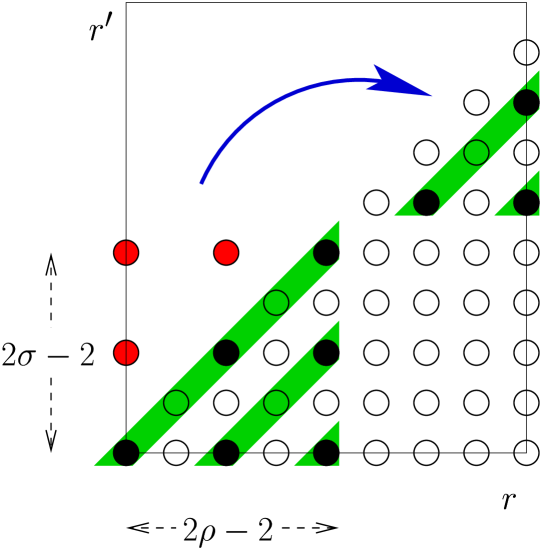
Figure 1: Boundary excitations for the boundary condition $(\rho,\sigma)$ fill a rectangle, or, after reflection, two triangles in the Kac table. In the large $m$ limit, they form bands with band-gaps around $2p=1$.

3.2 ZZ and FZZT branes at the Dirichlet points

Branes in the $c=1$ limit of minimal models with a discrete open string spectrum have also been constructed by Runkel and Watts (see also [35]). Actually, the branes that we obtained through the limit of minimal models when $s\in\mathbb{Z}$ are identical to the limit of $(s+1,1)$ branes in minimal models and hence to the discrete boundary conditions that were found by Runkel and Watts. We wish to point out that these branes may also be obtained from the so-called ZZ branes of Liouville theory. In general, the ZZ branes are labeled by a pair $(m,n)$ of positive integers and they possess the following 1-point functions,

$$\langle\Phi_{\alpha}(z,\bar{z})\rangle_{(m,n)}\ =\ -\frac{2^{3/4}2\pi ip}{\Gamma(1-2ibp)\Gamma(1-2ip/b)}\,\frac{\sinh 2\pi mp/b\,\sinh 2\pi nbp}{\sinh 2\pi p/b\,\sinh 2\pi bp}\,\frac{(\pi\mu\gamma(b^{2}))^{-ip/b}}{|z-\bar{z}|^{2h_{\alpha}}}\ \ .$$

If we send the parameter $b$ to $b=i$, these 1-point functions assume the following form

$$\langle\Phi_{p}(z,\bar{z})\rangle^{c=1}_{(m,n)}\ =\ -i(\pi\mu_{{\rm ren}})^{-p}2^{3/4}\frac{\sin 2\pi mp\,\sin 2\pi np}{\sin 2\pi p}\,\frac{1}{|z-\bar{z}|^{2p^{2}}}\ \ .$$

We can rewrite the coupling on the right hand side with the help of the trigonometric identity

$$\frac{\sin 2\pi mp\ \sin 2\pi np}{\sin 2\pi p}\ =\ \sum_{l=0}^{\min(m,n)-1}\,\sin 2\pi p(m+n-2l-1)$$

to read off the following geometric interpretation of the ZZ brane with label $(m,n)$ in the $c=1$ theory: it corresponds to an array of $\min(m,n)$ point-like branes that are distributed equidistantly such that the rightmost brane is located at $m+n$. This interpretation agrees with the geometry of branes that emerges from the coset construction of minimal models (see [36]).

With this in mind, we shall also be able to interpret our FZZT branes at the Dirichlet points $s\in\mathbb{Z}$. Let us recall that the $c=1$ limit of FZZT branes with integer label $s$ differs from the limit of minimal model branes. The precise relation between their two boundary states is given in eq. (3.5). On its right hand side we consider the difference of one-point couplings for two FZZT branes whose labels differ by two units. This is claimed to be the same as the one-point coupling to the discrete brane with label $(s+1,1)$. Therefore, the brane configuration that is associated to the FZZT brane with integer label $s$ contains an additional point-like object with transverse position parameter $s$ along the real line. The latter gets removed as we shift from $s$ to $s+2$. Our observation suggests to think of the $c=1$ FZZT branes with integer $s$ as being built up from discrete objects, or more specifically, as some half-infinite array of point-like objects. They occupy points with even or odd integer position $x$ in target space, depending on whether $s$ is odd or even. Changes of $s$ by one unit should therefore correspond to a simple translation of the entire array in the target space.

At least qualitatively, such an interpretation in terms of point-like branes appears consistent with our previous study of brane spectra on FZZT branes. In fact, we noticed before that their bands shrink to points when $s$ reaches integer values. Let us also stress that our geometric picture of the branes with integer $s$ is very similar to the interpretation of the Dirichlet points in the boundary Sine-Gordon model (see introduction).

More support for the proposed geometric pictures comes from considering spectra involving the ZZ branes in the $c=1$ theory. The annulus amplitude for two ZZ branes with labels $(m,n)$ and $(m^{\prime},n^{\prime})$ was found in [26] to be of the form

$$Z_{(m,n),(m^{\prime},n^{\prime})}(q) = \sum_{k=0}^{\min(m,m^{\prime})-1}\ \sum_{l=0}^{\min(n,n^{\prime})-1}\ \chi_{m+m^{\prime}-2k-1,n+n^{\prime}-2l-1}(q)$$

$$\mbox{where}\ \ \chi_{m,n}(q) = \eta^{-1}(q)\,\left(q^{-(m/b+nb)^{2}/4}-q^{-(m/b-nb)^{2}/4}\right)$$

$$\stackrel{{\scriptstyle b=i}}{{=}} \eta^{-1}(q)\,\left(q^{(m-n)^{2}/4}-q^{(m+n)^{2}/4}\right)\ \ .$$

Note that in the $c=1$ theory, excitations of the ZZ branes have non-negative conformal dimensions. Since $\chi_{m,n}$ are characters of irreducible Virasoro representations at $c=1$, the expression for the annulus amplitude coincides with what is obtained from the limit of Cardy type branes in unitary minimal models. A particularly simple case arises from setting $(m,n)=(1,1)$ and $(m^{\prime},n^{\prime})=(r,r)$,

$$Z_{(1,1),(r,r)}(q)\ =\ \chi_{r,r}(q)\ =\ \eta^{-1}(q)\,\left(1-q^{r^{2}}\right)\ \ .$$ (3.6)

According to our previous discussion, this amplitude encodes the spectrum of open strings between a single point-like brane and an array of length $2r$.

For the annulus amplitude between a ZZ brane $(m,n)$ and an FZZT brane at parameter $s$ one has

$$Z_{(m,n),s}(q) = \sideset{}{{}^{\prime}}{\sum}_{k=1-m}^{m-1}\ \sideset{}{{}^{\prime}}{\sum}_{l=1-n}^{n-1}\ \chi_{(s+i(k/b+lb))/2}(q)$$ (3.7)

$$\mbox{where}\ \ \chi_{p}(q) = \eta^{-1}(q)\,q^{p^{2}}\ \ .$$

Here, $\Sigma^{\prime}$ denotes a summation in steps of two. Let us point out that once more, the open string excitations between ZZ and FZZT branes have real, non-negative conformal dimensions when $b=i$. This is in contrast to the situation for $c\geq 25$ where the spectrum contains fields with complex dimensions if $n\neq 1$ or $m\neq 1$. The spectrum between the $(1,1)$ branes and an FZZT brane of parameter $s$ contains a single primary field with conformal dimension $h=s^{2}/4$, in perfect agreement with the construction from unitary minimal models. In fact, the construction of the $c=1$ brane we have proposed along with Cardy’s rule implies that there appears a single primary with Kac label given by eq. (3.4) in the corresponding spectrum of the $m^{th}$ minimal model. When we send $m$ to infinity, this field approaches a $c=1$ primary field with momentum

$$2p\ \sim\ [f_{s}m]+[s]-[f_{s}m]+\frac{1}{2(m+1)}\,(2[f_{s}m]+[s]+2)+\mathcal{O}(1/m^{2})\ \stackrel{{\scriptstyle m\rightarrow\infty}}{{\longrightarrow}}\ [s]+f_{s}\ =\ s\ \ .$$

Hence, there is perfect agreement between the annulus amplitudes in the $c=1$ limit of unitary minimal models and of Liouville theory.

Let us finally return to the analysis of our FZZT branes at the Dirichlet points. Since we already understand the effect of shifts in $s$, we can restrict the following discussion to the case $s=0$. We would like to probe this FZZT brane with the ZZ brane $(1,1)$. The amplitude (3.7) then becomes

$$Z_{(1,1),0}(q)\ =\ \eta^{-1}(q)\ =\ \lim_{r\rightarrow\infty}Z_{(1,1),(r,r)}(q)\ \ .$$

In the second equality, we inserted formula (3.6). This result nicely confirms our interpretation of the FZZT brane with label $s=0$ as an infinite array of point-like branes.

4 The boundary 2-point function

In this section we shall discuss how the boundary 2-point function of FZZT branes in Liouville theory can be continued to $c=1$. This will allow us to derive the exact boundary spectrum, in particular the position and width of the expected band gaps, from Liouville theory. Our results will confirm nicely the outcome of our previous discussion in the context of unitary minimal models.

Let us recall that the boundary 2-point functions for the FZZT branes in $c\geq 25$ Liouville theory are given by

$$\langle\Psi^{s_{1}s_{2}}_{\beta_{1}}(u_{1})\Psi^{s_{2}s_{1}}_{\beta_{2}}(u_{2})\rangle\ =\ |u_{1}-u_{2}|^{-2h_{\beta_{1}}}\,\left[\,\delta(Q_{b}-\beta_{1}-\beta_{2})+{\cal R}_{b}^{s_{1}s_{2}}(\beta_{1})\,\delta(\beta_{1}-\beta_{2})\right]\ \ .$$ (4.1)

The coefficient in front of the first term has been set to $1$ by an appropriate normalization of the boundary fields. Once this freedom of normalization has been fixed, the coefficient of the second term is entirely determined by the physics. It takes the form

$${\cal R}^{s_{1}s_{2}}_{b}(\beta)\ =\ \frac{(\pi\mu\gamma(b^{2})b^{2-2b^{2}})^{(Q_{b}-2\beta)/2b}}{S(\beta+i\tilde{s}|b)S(\beta-i\tilde{s}|b)S(\beta+i\tilde{s}_{1}|b)S(\beta+i\tilde{s}_{2}|b)}\,\frac{\Gamma_{2}(2\beta-Q_{b}|b)}{\Gamma_{2}(Q_{b}-2\beta|b)}$$ (4.2)

where $\tilde{s}=(s_{1}+s_{2})/2$ and $\tilde{s}_{i}=\tilde{s}-s_{i}$. The special function $S$ is constructed as a ratio of two Barnes double Gamma functions (see appendix A.2 for details). ${\cal R}$ is known as the reflection amplitude since it describes the phase shift of wave functions that occurs when open strings spanning between the FZZT branes with parameters $s_{1}$ and $s_{2}$ are reflected by the Liouville potential.

Our aim now is to continue these expressions to the $c=1$ model (see also [15] for a first attempt in this direction). Using once more the general formula (2) for the behavior of Barnes’ double Gamma function at $b\sim i$, it is not hard to see that the boundary reflection amplitude ${\cal R}$ of Liouville theory vanishes outside a discrete set of open string momenta. This behavior is unacceptable since it does not allow for a sensible physical interpretation. Actually, it does not originate from the physics of the model but rather from an inappropriate choice of the limiting procedure. To see this we recall that the boundary spectrum of the theory is expected to develop gaps of finite width. For such gaps to emerge from Liouville theory, it is necessary that the corresponding states in the Liouville model become non-normalizable. But our normalization of boundary fields was chosen such that all states in the boundary theory have unit norm. Hence, the normalization we have chosen above is clearly not appropriate for the limit we are about to take.

There exists a distinguished normalization of the boundary fields in which the reflection amplitude of the boundary theory becomes trivial. Since the usual ‘Liouville wall’ ceases to exist at the point $b=i$, the trivialization of the boundary reflection amplitude seems quite well adapted to our physical setup. Explicitly, the new normalization of the boundary fields is given by [25, 30],

$$\tilde{\Psi}^{s_{1}s_{2}}_{\beta}(u)\ =\ g_{\beta}^{s_{1}s_{2}}\Psi^{s_{1}s_{2}}_{\beta}(u)\ \ ,$$ (4.3)

with

$$g_{\beta}^{s_{1}s_{2}}\ =\ \frac{\big{(}\pi\mu\gamma(b^{2})b^{2-2b^{2}}\big{)}^{\frac{\beta}{2b}}}{\Gamma_{2}(Q_{b}-\beta-i\tilde{s}|b)}\frac{\Gamma_{2}(Q_{b}|b)\Gamma_{2}(Q_{b}-2\beta|b)\Gamma_{2}(Q_{b}+is_{1}|b)\Gamma_{2}(Q_{b}-is_{2}|b)}{\Gamma_{2}(Q_{b}-\beta+i\tilde{s}_{2}|b)\Gamma_{2}(Q_{b}-\beta+i\tilde{s}_{1}|b)\Gamma_{2}(Q_{b}-\beta+i\tilde{s}|b)}\ \ .\ \$$

It is straightforward to rewrite the 2-point function in terms of the fields $\tilde{\Psi}^{s_{1}s_{2}}_{\beta}(u)$. The result is

$$\langle\tilde{\Psi}^{s_{1}s_{2}}_{\beta_{1}}(u_{1})\,\tilde{\Psi}^{s_{2}s_{1}}_{\beta_{2}}(u_{2})\rangle \sim \frac{\left(\pi\mu\gamma(b^{2})\right)^{(Q_{b}/2-\beta_{1}-i\tilde{s})/b}}{|u_{1}-u_{2}|^{2h_{\beta_{1}}}}\ C_{b}^{-1}(\beta_{1},\sigma_{1},\sigma_{2})\,\times$$

$$\times\,\frac{\Gamma(1+2ibp_{1})\Gamma(2ib^{-1}p_{1})}{\Gamma(1-ibs_{1})\Gamma(-ib^{-1}s_{1})\Gamma(1-ibs_{2})\Gamma(-ib^{-1}s_{2})}\ \left[\,\delta(Q_{b}-\beta_{1}-\beta_{2})+\delta(\beta_{1}-\beta_{2})\,\right]\ \ .$$

Here we use $\beta=Q_{b}/2+ip$ and the term $C_{b}$ in the denominator denotes the bulk 3-point couplings of Liouville theory evaluated at the points $\beta_{1}$ and $\sigma_{i}=Q_{b}/2+is_{i}/2$. In writing this expression we have omitted a factor that is constant in the momentum $p_{1}$ and invariant under the exchange of $s_{1}$ and $s_{2}$ since this can easily be absorbed in a redefinition of the boundary fields.

When rewritten in the new normalization, the only nontrivial term in the expression (4) is the bulk 3-point function. Hence, we can use the results of [27] (see also section 2) to continue the boundary 2-point function to $c=1$. Note, however, that the bulk 3-point coupling needs to be inverted. This is possible whenever it is non-zero. Since the coupling $C_{c=1}(\beta,\sigma_{1},\sigma_{2})$ vanishes whenever the factor $P(2p,s_{1},s_{2})$ does, we conclude that boundary fields $\Psi^{s_{1}s_{2}}_{\beta}$ exist for $p\in{\cal S}_{s_{1}s_{2}}\subset\mathbb{R}$ where

$${\cal S}_{s_{1}s_{2}}\ :=\ \{p\in\mathbb{R}\,|P(2p,s_{1},s_{2})\neq 0\}\ \ .$$

Fields which are labeled by momenta outside this range ${\cal S}_{s_{1}s_{2}}$ do not correspond to normalizable states of the model. On a single brane with label $s=s_{1}=s_{2}$ we obtain in particular

$${\cal S}_{ss}\ =\ {\cal S}_{s}\ =\{p\in\mathbb{R}\,|\,-\min(f_{s},1-f_{s})<p<\min(f_{s},1-f_{s})\ \mod\ 1\,\}\ \ .$$

Here, $f_{s}=s-[s]$ denotes the fractional part of the boundary parameter as before. This is exactly the same spectrum we found in our discussion of boundary conditions in the $c=1$ limit of unitary minimal models !

Our result for the 2-point functions of boundary fields in the spectrum of the model is given by

$$\langle\tilde{\Psi}^{s_{1}s_{2}}_{p_{1}}(u_{1})\tilde{\Psi}^{s_{2}s_{1}}_{p_{2}}(u_{2})\rangle^{c=1} \sim \frac{e^{-Q(iP_{1},is_{1}/2,is_{2}/2)}}{|u_{1}-u_{2}|^{2p^{2}_{1}}}\left|\frac{\sin\pi s_{1}\,\sin\pi s_{2}}{\sin 2\pi p_{1}}\right|\,\left[\delta(p_{1}+p_{2})+\delta(p_{1}-p_{2})\right]$$

$$\mbox{ where }\ \ e^{Q(\alpha_{1},\alpha_{2},\alpha_{3})} := \frac{\Upsilon(1+2i\tilde{\alpha}|1)}{\Upsilon(1|1)}\ \prod_{j=1}^{3}\,\frac{\Upsilon(1+2i\tilde{\alpha}_{j})}{\Upsilon(1+2i\alpha_{j})}\ \ .$$

In a final step, we change the normalization of the fields $\tilde{\Psi}$ in the $c=1$ theory again so that they possess unit norm,

$$\Psi^{s_{1}s_{2}}_{p}(u)\ :=\ \tilde{g}_{p}^{s_{1}s_{2}}\tilde{\Psi}^{s_{1}s_{2}}_{p}(u)\ \ ,$$ (4.5)

with

$$\tilde{g}_{p}^{s_{1}s_{2}}\ =\ \frac{\left(\pi\mu_{\text{ren}}\right)^{-p/2}}{\Gamma(-2p)}\,\frac{\Gamma_{2}(1|1)\Gamma_{2}(1+2p|1)\Gamma_{2}(1-s_{1}|1)\Gamma_{2}(1+s_{2}|1)\Gamma(s_{1})\Gamma(1-s_{2})}{\Gamma_{2}(1+p+\tilde{s}|1)\Gamma_{2}(1+p-\tilde{s}_{1}|1)\Gamma_{2}(1+p-\tilde{s}_{2}|1)\Gamma_{2}(1+p-\tilde{s}|1)}\ \ .$$

In an abuse of notation, we have denoted the normalized boundary fields of the $c=1$ model by the same letter $\Psi$ as in $c\geq 25$ Liouville theory. Nevertheless it important to keep in mind that they are not justs limits of the corresponding fields in ordinary Liouville theory. After this final change of normalization, the boundary 2-point functions take the form

$$\langle\Psi^{s_{1}s_{2}}_{p_{1}}(u_{1})\Psi^{s_{2}s_{1}}_{p_{2}}(u_{2})\rangle^{c=1}\ =\ \frac{{\cal N}^{s_{1}s_{2}}(p)}{|u_{1}-u_{2}|^{2p^{2}_{1}}}\ \left[\delta(p_{1}+p_{2})+{\cal R}^{s_{1}s_{2}}_{c=1}(p_{1})\delta(p_{1}-p_{2})\right]$$ (4.6)

$$\mbox{ where }\ \ {\cal R}^{s_{1}s_{2}}_{c=1}(p)\ =\ {\cal R}^{is_{1}\ is_{2}}_{c=25}(1-p)^{-1}\ \ \mbox{and }\ \ {\cal{N}}^{s_{1}s_{2}}(p)\ =\ -2\epsilon p_{1}(-1)^{[2p_{1}]+[s_{1}]+[s_{2}]}$$

for all $p_{1},p_{2}\in{\cal S}_{s_{1}s_{2}}$. Note that we have been able to express the “boundary reflection amplitude” of the $c=1$ theory through the corresponding quantity of the $c=25$ model. We shall comment on this interesting outcome of our computation in the section 6.

5 The bulk-boundary coupling constants

Our final aim is to compute the bulk-boundary couplings of the $c=1$ boundary Liouville models. For Liouville theory with real $b$, expressions for these couplings were provided by Hosomichi in [24]. We shall depart from these formulas to derive the corresponding couplings in the $c=1$ model. The analysis turns out to be rather intricate. Nevertheless, the final answer is in some sense simpler than for $c\geq 25$.

Let us begin by reviewing Hosomichi’s formula for the bulk-boundary correlation function

$$\langle\Phi_{\alpha}(z,\bar{z})\tilde{\Psi}^{ss}_{\beta}(u)\rangle\ =\ |z-\bar{z}|^{h_{\beta}-2h_{\alpha}}|z-u|^{-2h_{\beta}}\tilde{B}(\alpha,\beta,s)$$

of an extended branes labeled by a parameter $s$. In our normalization (4.3) for the boundary fields $\tilde{\Psi}$ the couplings $\tilde{B}$ read

$$\tilde{B}(\alpha,\beta,s)\ =\ 2\pi(\mu\pi\gamma(b^{2})b^{2-2b^{2}})^{\frac{1}{2b}(Q_{b}-2\alpha)}\,I(\alpha,\beta,s,b)\\[5.69054pt] \times\ \frac{\Gamma_{2}(Q_{b}-\beta|b)\Gamma_{2}(2Q_{b}-2\alpha-\beta|b)\Gamma_{2}(2\alpha-\beta|b)\Gamma_{2}(Q_{b}+is|b)\Gamma_{2}(Q_{b}-is|b)}{\Gamma_{2}(Q_{b}-\beta-is|b)\Gamma_{2}(Q_{b}-\beta+is|b)\Gamma_{2}(\beta|b)\Gamma_{2}(2\alpha|b)\Gamma_{2}(Q_{b}-2\alpha|b)}$$ (5.1)

where $I(\alpha,\beta,s)$ is given by the integral

$$I(\alpha,\beta,s,b)\ =\ \int_{-\infty}^{\infty}dt\,e^{2\pi ist}\ \frac{S(\tfrac{\beta+2\alpha-Q_{b}}{2}+it|b)S(\tfrac{\beta+2\alpha-Q_{b}}{2}-it|b)}{S(\tfrac{2\alpha-\beta+Q_{b}}{2}+it|b)S(\tfrac{2\alpha-\beta+Q_{b}}{2}-it|b)}\ \ .$$ (5.2)

While sending $b$ to $b=i$, an infinite number of poles and zeroes of the integrand approach the integration path. It turns out to be more convenient to evaluate the integral by Cauchy’s theorem. For $s>|\text{Im}\,\beta|$ we can close the integration contour and rewrite the sum over residues as a combination of basic hypergeometric series (see appendix A.1),

$$I(\alpha,\beta,s,b)\ =\ {}_{2}\Phi_{1}\big{(}e^{2\pi ib(\beta+2\alpha-Q_{b})},e^{2\pi ib\beta},e^{4\pi ib\alpha};e^{2\pi ib^{2}};e^{-2\pi ib(\beta-Q_{b}-is)}\big{)}$$

$$\quad\times\ {}_{2}\Phi_{1}\big{(}e^{-2\pi ib^{-1}(\beta+2\alpha-Q_{b})},e^{-2\pi ib^{-1}\beta},e^{-4\pi ib^{-1}\alpha};e^{-2\pi ib^{-2}};e^{2\pi ib^{-1}(\beta-Q_{b}+is)}\big{)}$$

$$\quad\times\ e^{-\pi s(\beta+2\alpha-Q_{b})}S(\beta|b)S(\beta+2\alpha-Q_{b}|b)S(Q_{b}-2\alpha|b)+\ (\alpha\rightarrow Q_{b}-\alpha)\ \ .$$ (5.3)

Our previous results allow us to estimate the behavior of the double Gamma functions and its close relative $S$ in the vicinity of $b=i$. But the function ${}_{2}\Phi_{1}(A,B,C;\tilde{q};z)$ has not appeared in our discussion before. Hence, in order to continue our analysis, we need to study the basic hypergeometric series in the limit when the parameter $\tilde{q}$ approaches $\tilde{q}=1$. We shall begin with a separate treatment of the two factors ${}_{2}\Phi_{1}$ before we combine the results to address the full coupling $\tilde{B}$.

In dealing with one of the basic hypergeometric series, the basic idea is to approximate the series (we denote the summation parameter by $k$) through an integral and to evaluate the latter using a saddle-point analysis. We will not give a rigorous derivation but shall content ourselves with a rough sketch of the argument. This will help to understand the main features of our final formulas. Let us introduce the variable $y=\tilde{q}^{k}$. Using the asymptotic behavior of the q-Pochhammer symbols (see appendix B) we obtain

$$_{2}\Phi_{1}(A,B,C;\tilde{q};z)\ \sim\ \frac{1}{\sqrt{-2\pi\log\tilde{q}}}\int\frac{dy}{y}e^{\frac{1}{\log\tilde{q}}h(y)}f(y)$$ (5.4)

where

$$h(y)\ =\ h(A,B,C,z,y) = \text{Li}_{2}(A)-\text{Li}_{2}(Ay)+\text{Li}_{2}(B)-\text{Li}_{2}(By)$$

$$-\text{Li}_{2}(C)+\text{Li}_{2}(Cy)-\text{Li}_{2}(1)+\text{Li}_{2}(y)+\log y\,\log z\ \ ,$$

and

$$f(y)\ =\ f(A,B,C,z,y)\ =\ \left(\frac{(1-A)(1-B)(1-Cy)}{(1-Ay)(1-By)(1-C)(1-y)}\right)^{1/2}\ \ .$$ (5.5)

The asymptotics of the integral in eq. (5.4) can be determined by the method of steepest descent. The leading contribution comes from saddle-points $y_{i}$, i.e. from points satisfying the condition $h^{\prime}(y_{i})=0$. An elementary computation shows that such saddle-points are obtained as a solution of the quadratic equation

$$z(1-Ay)(1-By)\ =\ (1-Cy)(1-y)\ \ .$$ (5.6)

Once we have understood which saddle-points $y_{i}$ contribute to the integral, we end up with an expansion of the form

$${}_{2}\Phi_{1}(A,B,C;\tilde{q},z)\ \sim\ \sum_{i}\frac{f(y_{i})}{y_{i}\sqrt{h^{\prime\prime}(y_{i})}}e^{\frac{1}{\log\tilde{q}}h(y_{i})}\ \ .$$

The most difficult part, however, is to find the right saddle-points. To begin with, the saddle-point equation (5.6) has two different solutions, at least for generic choice of the momenta. But this is not the full story since the function $h$ is a complex function with branch-cuts. Hence, the description of the saddle point $y_{i}$ is not complete before we have specified on which branch the relevant saddle-point is located. We were not able to solve the problem in full generality, but for the combination of parameters in the problem at hand, we could find the saddle-points through a comparison with numerical studies (Mathematica).

Let us state the result for the first q-hypergeometric function appearing in eq. (5.3). Here, the parameter $\tilde{q}$ is $e^{2\pi ib^{2}}$ and thus the prefactor $1/\log\tilde{q}$ of $h$ in the exponent becomes $-\frac{1}{\epsilon}-\frac{i}{2\pi}$, where $\epsilon=2\pi iQ_{b}/b$ as introduced in section 2. Note that the arguments $A,B,C$ and $z$ depend on $b$ and thus on $\epsilon$ and hence they need to be expanded around $\epsilon=0$. We shall use the symbols $A_{0},B_{0},C_{0}$ and $z_{0}$ to denote the leading terms, i.e.

$$A_{0}\ =\ B_{0}C_{0}\ \ ,\ \ B_{0}\ =\ e^{-2\pi ip_{\beta}}\ \ ,\ \ C_{0}\ =\ e^{-4\pi ip_{\alpha}}\ \ ,\ \ z_{0}\ =\ e^{-2\pi i(s-p_{\beta})}\ \ ,$$

where we have set $\alpha=Q_{b}/2+ip_{\alpha}$ and $\beta=Q_{b}/2+ip_{\beta}$. Since the function $h$ in the exponential comes with an extra factor $1/\epsilon$, the sub-leading term in the $\epsilon$-expansion of $h$ contributes an extra factor which we shall combine with $f$ into a new function $g$. Before we spell out our results on the saddle points, we also have to specify the branch we use for $\log z$. We found it most convenient to choose $\log z\to 2\pi i(p_{\beta}-[p_{\beta}]-s+[s])$. In the end we obtain,

$${}_{2}\Phi_{1}\big{(}e^{2\pi ib(\beta+2\alpha-Q_{b})},e^{2\pi ib\beta},e^{4\pi ib\alpha};e^{2\pi ib^{2}};e^{-2\pi ib(\beta-Q_{b}-is)}\big{)}\ \sim\ \sum_{i=\pm}\frac{g(y_{i})}{y_{i}\sqrt{h^{\prime\prime}(y_{i})}}e^{\big{(}-\frac{1}{\epsilon}-\frac{i}{2\pi}\big{)}h(y_{i})}$$

with

$$g(y)\ =\ \left(\frac{1-A_{0}}{1-A_{0}y}\right)^{-p_{\alpha}-p_{\beta}/2}\left(\frac{1-B_{0}}{1-B_{0}y}\right)^{-p_{\beta}/2}\left(\frac{1-C_{0}}{1-C_{0}y}\right)^{p_{\alpha}+1/2}(1-y)^{-1/2}y^{\frac{1+s-p_{\beta}}{2}}\ \ .$$

The two solutions of the saddle-point equation are denoted by $y_{\pm}$, and they are given explicitly by

$$y_{\pm}\ =\ y_{\pm}(p_{\alpha},p_{\beta},s)$$

$$\ \ =\ \left\{\begin{array}[]{l}e^{\pi i(2p_{\alpha}+p_{\beta})}\frac{\cos(2\pi p_{\alpha})\sin(\pi s)}{\sin(\pi(p_{\beta}+s))}\bigg{(}1\mp i\tan(2\pi p_{\alpha})\sqrt{1-\frac{\sin(\pi p_{\beta})^{2}}{\sin(\pi s)^{2}\sin(2\pi p_{\alpha})^{2}}}\bigg{)}\\[2.84526pt] \quad\quad\text{for}\ |\sin(\pi p_{\beta})|<|\sin(\pi s)\sin(2\pi p_{\alpha})|\\[8.53581pt] e^{\pi i(2p_{\alpha}+p_{\beta})}\frac{\cos(2\pi p_{\alpha})\sin(\pi s)}{\sin(\pi(p_{\beta}+s))}\bigg{(}1\mp\sqrt{\frac{\sin^{2}(\pi p_{\beta})-\sin^{2}(2\pi p_{\alpha})\sin^{2}(\pi s)}{\sin^{2}(\pi s)\cos^{2}(2\pi p_{\alpha})}}\bigg{)}\\[2.84526pt] \quad\quad\text{for}\ |\sin(\pi s)|\geq|\sin(\pi p_{\beta})|\geq|\sin(\pi s)\sin(2\pi p_{\alpha})|\\[8.53581pt] e^{\pi i(2p_{\alpha}+p_{\beta})}\frac{\cos(2\pi p_{\alpha})\sin(\pi s)}{\sin(\pi(p_{\beta}+s))}\bigg{(}1\mp\frac{\sin(\pi(s+2p_{\alpha}))}{\sin(\pi s)\cos(2\pi p_{\alpha})}\sqrt{\frac{\sin^{2}(\pi p_{\beta})-\sin^{2}(2\pi p_{\alpha})\sin^{2}(\pi s)}{\sin^{2}(\pi(s+2p_{a}))}}\bigg{)}\\[2.84526pt] \quad\quad\text{for}\ |\sin(\pi p_{\beta})|\geq|\sin(\pi s)|\end{array}\right.$$

The last of these three different cases concerns the band gaps, i.e. momenta $p_{\beta}\not\in{\cal S}_{s}$. The first two cases, on the other hand, apply to the bands so that all bands appear to be split into an inner (first case) and an outer (second case) region, depending on the value of the bulk momentum $p_{\alpha}$. Analyzing the limit in the outer part of the bands turns out to be the most difficult task because the two saddle-points $y_{\pm}$ are of the same order, i.e. $\text{Re}\,h(y_{+})=\text{Re}\,h(y_{-})$, and there are at least some subsets in momentum space where they both contribute. Within the inner region and the gap, the saddle-point $y_{+}$ dominates so that only the summand $i=+$ remains in our asymptotic expansion. The exact description of our findings for the intermediate region is rather cumbersome. Fortunately, the distinction between inner and outer parts of the band disappears once we combine our two basic hypergeometric series into the bulk-boundary coupling. Since our main goal is to provide a formula for the $c=1$ limit of $\tilde{B}$, we shall not attempt to present our findings for ${}_{2}\Phi_{1}$ in the outer region. Instead, let us recall from above that we also need to specify the branch on which the saddle-points sit. The prescription is as follows: If $|y_{i}|>1$, then we choose the branch by moving it from the fundamental branch first to $|y_{i}|\pm i0_{+}$, infinitesimally above/below the real axis depending on whether the fractional part $s-[s]$ is greater or smaller than $1/2$. Then we move it on the shortest arc to $y_{i}$.

Having completed the analysis for the first hypergeometric function we now turn to the second for which an analogous investigation gives the following results,

$$\tilde{h}(y)\ =\ h(A_{0},B_{0},C_{0},z_{0}^{-1}B_{0}^{-2},y)$$

and

$$\tilde{g}(y)\ =\ \left(\frac{1-A_{0}}{1-A_{0}y}\right)^{p_{\alpha}+p_{\beta}/2}\left(\frac{1-B_{0}}{1-B_{0}y}\right)^{p_{\beta}/2}\left(\frac{1-C_{0}}{1-C_{0}y}\right)^{-p_{\alpha}+1/2}(1-y)^{-1/2}y^{\frac{1+s+p_{\beta}}{2}}\ \ .$$

Note that in this case $\frac{1}{\log\tilde{q}}$ is directly given by $-\frac{1}{\epsilon}$. The relevant saddle-points are

$$\tilde{y}_{\pm}\ =\ y_{\pm}(p_{\alpha},p_{\beta},-s)\ \ .$$

Our discussion of the three different cases and the choice of branches carries over from the previous discussion without any significant changes.

Before we return to the study of $\tilde{B}$ it is necessary to make one more important observation which relates the two saddle-points $y_{\pm}$ and $\tilde{y}_{\pm}$. It is not difficult to see that $(A_{0}\tilde{y}_{\pm})^{-1}$ solves the saddle-point equation (5.6) of $y_{\pm}$. Indeed we find for $p_{\beta}\in{\cal S}_{s}$ that $y_{\pm}=(A_{0}\tilde{y}_{\mp})^{-1}$. This fact along with some simple formulas in appendix A.3 allows to re-express the final formulas entirely in terms of $y_{+}(p_{\alpha},p_{\beta},s)$.

Now we have all ingredients at our disposal to analyze the asymptotic behavior of the bulk-boundary correlator. We must combine the divergences coming from the q-hypergeometric functions with the divergences of the prefactors in eq. (5.1). Since we know already that boundary fields with $p_{\beta}\not\in{\cal S}_{s}$ do not exist, we can restrict our evaluation of $\tilde{B}$ to the inner and outer band regions (see discussion above).

In the inner region, only one saddle-point contributes and the divergent terms may be determined easily from the formulas we have provided. It then turns out that they cancel each other thanks to a rather non-trivial dilogarithm identity which is attributed to Ray [37]. For convenience we state Ray’s identity in appendix A.3 (eq. (A.3)). Hence, we are left with a finite result. After a tedious but elementary computation we obtain

$$\lim_{b\to i}\tilde{B}(\alpha,\beta,s)\ =\ 4\pi i(\pi\mu_{\text{ren}})^{-p_{\alpha}}e^{-\pi is(p_{\beta}+1)}\,\sin\pi s\ \bigg{(}\frac{e^{-2\pi ip_{\alpha}(s+1)}}{1-e^{-4\pi ip_{\alpha}}}\times$$

$$\ \times\ \frac{g(y_{+})^{2}e^{-\frac{ih(y_{+})}{2\pi}}}{y_{+}^{2}h^{\prime\prime}(y_{+})}\ \frac{\Gamma_{2}(1+p_{\beta}+s|1)\Gamma_{2}(1+p_{\beta}-s|1)\Gamma_{2}(1-2p_{\alpha}|1)^{2}}{\Gamma_{2}(1-2p_{\alpha}-p_{\beta}|1)\Gamma_{2}(1-2p_{\alpha}+p_{\beta}|1)\Gamma_{2}(1-s|1)\Gamma_{2}(1+s|1)}$$

$$\quad\quad\quad\ -\ (p_{\alpha}\to-p_{\alpha})\bigg{)}\ \$$

where $y_{+}=y_{+}(p_{\alpha},p_{\beta},s)$. In the derivation we used the fact that $y_{+}$ and $(A_{0}\tilde{y}_{+})^{-1}=y_{-}$ are the two solutions of the same quadratic saddle-point equation along with a few elementary identities which we list in appendix A.3.

Within the outer regions of the bands, the q-hypergeometric functions can have contributions from both saddle-points. It is possible to show that out of the four possible terms in our product of two q-hypergeometric functions, only two appear at any point in momentum space. Moreover, after the divergences of the prefactors have been taken into account, only one of the two terms is free of divergences. The other keeps a rapidly oscillating factor. The cancellation is again due to Ray’s identity and the finite contributions come from the combination $(y_{+},\tilde{y}_{+})$. In the end, the result for the outer region of the band is therefore given by the same formula as for the inner region.

It now remains to change the normalization of our boundary fields. We pass from the fields $\tilde{\Psi}$ to $\Psi$ using the prescription (4.5), as before. Our result then reads

$$B(p_{\alpha},p_{\beta},s)\ =\ 4\pi^{2}i(\pi\mu_{\text{ren}})^{-p_{\alpha}-p_{\beta}/2}e^{-\pi is(p_{\beta}+1)}\,\Gamma^{-1}(-2p_{\beta})$$

$$\quad\times\ \Big{(}\frac{e^{-2\pi ip_{\alpha}(s+1)}}{1-e^{-4\pi ip_{\alpha}}}\frac{g(y_{+})^{2}e^{-\frac{ih(y_{+})}{2\pi}}}{y_{+}^{2}h^{\prime\prime}(y_{+})}\frac{\Gamma_{2}(1|1)\Gamma_{2}(1+2p_{\beta}|1)\Gamma_{2}(1-2p_{\alpha}|1)^{2}}{\Gamma_{2}(1-2p_{\alpha}-p_{\beta}|1)\Gamma_{2}(1-2p_{\alpha}+p_{\beta}|1)\Gamma_{2}(1+p_{\beta}|1)^{2}}$$

$$\quad\quad\quad\ -\ (p_{\alpha}\to-p_{\alpha})\Big{)}\ \ .$$

This is the formula we anticipated in the introduction. For a direct comparison one has to employ the integral representation (A.2) of Barnes’ double Gamma function.

Before we conclude this section, we would like to comment briefly on the band-gaps. Actually, we can use the analysis of the bulk-boundary couplings to confirm our previous statement that boundary fields $\Psi^{ss}_{p_{\beta}}$ with $p_{b}\not\in{\cal S}_{s}$ decouple from the theory. To this end, we shall focus on the coefficients $A$ of the bulk boundary operator product expansion rather than the couplings $B$. The former are related to latter by multiplication with the boundary 2-point function. Our claim is that the coefficients $A_{b=i}$ vanish within the band-gaps. As we have seen before, the 2-point function contributes a factor that diverges when $p_{\beta}\not\in{\cal S}_{s}$. With the help of our asymptotic expansion formulas in this section it is possible to show that the couplings $B$ always diverge slower. Hence, boundary fields whose momenta lie in the gaps cannot be excited when a bulk field approaches the boundary.

6 Conclusion and open problems

In this work we have constructed boundary conditions of the Euclidean $c=1$ Liouville model. In particular we argued that there exists a family of boundary conditions that is parametrized by one real parameter $s\in\mathbb{R}$. We provided explicit expressions for their boundary states (see eq. (3.2)), the boundary 2-point function (4.6,4.2), and the bulk-boundary coupling (1). The only quantity that we are missing for a complete solution of the model is the boundary 3-point coupling. In the case of Liouville theory, the corresponding formulas have been found by Ponsot and Teschner in [25]. We believe that the analysis of their $c=1$ limit can proceed along the lines of the studies we have presented in section 5, but obviously this program remains to be carried out in detail.

A crucial ingredient in our study was the formula (2) for the asymptotics of Barnes’ double Gamma function. In section 2, the latter enabled us to provide a new derivation of the bulk couplings in the $c=1$ Liouville model. Our approach here is simpler and more general than the one that was developed in [27]. With this technical progress it is now also possible to calculate the bulk couplings of non-rational conformal field theories with $c<1$. In contrast to the $c=1$ case, the models with $c<1$ are certainly non-unitary. We will comment on the results and their relation with minimal models elsewhere. Possible applications of such developments include the 2-dimensional cigar background with $0\leq k\leq 2$ [38] and similar limits of the associated boundary theories [39].

All this research, however, was mainly motivated by the desire to construct an exact conformal field theory model for the homogeneous condensation of open string tachyons, such as the tachyon on an unstable D0 brane in type IIB theory. As we explained in the introduction, the underlying world-sheet theory is a Lorentzian version of the model we have considered in this work. But since the couplings of our theory are not analytic in the momenta (with the boundary state being the only exception), this Lorentzian theory cannot be obtained by a simple Wick rotation from the solution we described here. Instead, it was suggested in [27] to perform the Wick rotation before sending $b$ to its limiting value $b=i$. Such a prescription makes sense because the couplings of Liouville theory are analytic in the momenta as long as $b$ is not purely imaginary. It is certainly far from obvious that the Wick rotated couplings again possess a well-defined $b=i$ limit. Preliminary studies of this issue show that our analysis of the boundary 2-point function extends to the Lorentzian case. In the time-like model, the spectrum of boundary fields is continuous (there are no gaps) and their 2-point function is still given by eq. (4.6) with a reflection amplitude

$${\cal R}^{s_{1}s_{2}}_{c=1}(x)\ =\ {\cal R}^{is_{1}\ is_{2}}_{c=25}(1+ix)^{-1}\ \ .$$

This result does not agree with the proposal in [15]. Note, however, that in the Lorentzian case the correlation functions can depend on the details of how $b$ approaches $b=i$. Such a behavior might be related to a choice of vacuum. Let us also anticipate that consistency of our expression for the boundary 2-point coupling with the half-brane boundary states [33, 15] can be checked by means of the modular bootstrap. A related observation, though with a somewhat problematic domain of open string momenta, has also been made in [41]. Concerning the bulk-boundary coupling, our investigations are not complete yet. But before having worked out the expression in the Lorentzian model, it is worthwhile comparing our formula (1) for the bulk-boundary coupling with a corresponding expression in the time-like theory that was suggested recently in [42] (eq. [4.14] of that paper). In fact, the exponential in the second line of our formula is identical to a corresponding factor in the work of Balasubramanian et. al. It will be interesting to determine the other factors through our approach. We shall return to this issue in a forthcoming publication.

Acknowledgements: We would like to thank V. Balasubramanian, P. Etingof, J. Fröhlich, M.R. Gaberdiel, K. Graham, G. Moore, B. Ponsot, I. Runkel, J. Teschner and G. Watts for very helpful discussions and some crucial remarks. Part of this research has been carried out during a stay of VS with the String Theory group of Rutgers University and of both authors at the Erwin Schroedinger Institute for Mathematical Physics in Vienna. We are grateful for their warm hospitality during these stays.

Appendix A Some background on special functions

In this first appendix we collect a few results on the special functions which appear in the analysis of the $c=1$ boundary Liouville model. We shall start with some q-deformed special functions and then introduce Barnes’ double Gamma functions and certain closely related special functions. Dilogarithms and some of their properties are finally reviewed in the third subsection.

A.1 q-Pochhammer symbols and q-hypergeometric functions

One of the most basic objects in the theory of q-deformed special functions is the finite q-Pochhammer symbol (see e.g. [43])

$$\big{(}a;\tilde{q}\big{)}_{k}\ :=\ \prod_{n=0}^{k-1}(1-a\tilde{q}^{n})\ \ .$$

Its limit for $k\to\infty$ exists for $|\tilde{q}|<1$ and is denoted by

$$\big{(}a;\tilde{q}\big{)}_{\infty}\ =\ \prod_{n=0}^{\infty}(1-a\tilde{q}^{n})\ \ .$$ (A.1)

The tilde is used to avoid confusion with our convention for $q$ in the rest of the text.

With the help of the the finite q-Pochhammer symbol we can now introduce the basic hypergeometric series ${}_{2}\Phi_{1}$. This q-deformation of the hypergeometric function ${}_{2}F_{1}$ is defined as

$${}_{2}\Phi_{1}(A,B,C;\tilde{q};z)\ =\ \sum_{k=0}^{\infty}\frac{\big{(}A;\tilde{q}\big{)}_{k}\,\big{(}B;\tilde{q}\big{)}_{k}}{\big{(}C;\tilde{q}\big{)}_{k}\,\big{(}\tilde{q};\tilde{q}\big{)}_{k}}z^{k}\ \ .$$

The interested reader can find many basic properties of these functions in the literature (see e.g. [44, 43]). All the properties we need in the main text are stated and derived there.

A.2 Barnes’ double Gamma function and related functions

Barnes’ double $\Gamma$-function $\Gamma_{2}(x|b)$ is defined for $x\in\mathbb{C}$ and complex $b$ with $\text{Re}\,b\not=0$ (see [45]), and can be represented by an integral (for $\text{Re}\,x>0$),

$$\log\Gamma_{2}(x|b)\ =\ -\int_{0}^{\infty}\frac{{\rm d}t}{t}\Bigg{(}\frac{e^{-Q_{b}t/2}-e^{-xt}}{(1-e^{-bt})(1-e^{-t/b})}+\frac{(Q_{b}/2-x)^{2}}{2}e^{-t}+\frac{Q_{b}/2-x}{t}\Bigg{)}\ \ ,$$ (A.2)

whenever $\text{Re}\,x>0$. Here we have also introduced the symbol

$$Q_{b}=b+b^{-1}\ \ .$$

Throughout the main text, we often use the following special combinations of double Gamma functions,

$$\Upsilon(x|b) = \Gamma_{2}(x|b)^{-1}\,\Gamma_{2}(Q_{b}-x|b)^{-1}$$ (A.3)

$$S(x|b) = \Gamma_{2}(x|b)\,\Gamma_{2}(Q_{b}-x|b)^{-1}\ \ .$$ (A.4)

For the latter, we would also like to spell out an integral representation that easily follows from the formula (A.2) above,

$$\log S(x|b)\ =\ \int_{0}^{\infty}\frac{dt}{t}\bigg{(}\frac{\sinh(Q_{b}-2x)t}{2\sinh(bt)\sinh(t/b)}-\frac{Q_{b}/2-x}{t}\bigg{)}\ \ .$$

This representation is valid for $|\text{Re}\,x|<\text{Re}\,Q_{b}$. Let us also note that $S$ is unitary in the sense that $S(x|b)S(Q_{b}-x|b)=1$ The function $S$ is also closely related to Ruijsenaars’ hyperbolic Gamma function $\Gamma_{h}$ (see [46]),

$$S(x)\ =\ \Gamma_{h}\big{(}i(x-Q_{b}/2)\big{)}\ \ .$$

Many further properties of double Gamma functions, in particular on the position of their poles and shift properties, can be found in the literature (see e.g. [47]).

Here we would like to prove one relation that involves the q-Pochhammer symbols we introduced in the previous subsection. To this end, we depart from the integral representation (A.2). Let us denote the integrand in formula (A.2) by $f(t,x,b)$, s.t.  $\log\Gamma_{2}(x|b)=-\int_{0}^{\infty}dt\,f(t,x,b)$. The function $f$ has the property

$$if(it,x,b)\ =\ -f(t,-ib+ix,-ib)+\frac{(\tfrac{Q_{b}}{2}-x)^{2}}{2t}(e^{-it}-e^{-t})\ \ .$$ (A.5)

We evaluate the integral by closing the contour in the first quadrant,

$$\log\Gamma_{2}(x|b)\ =\ -i\int_{0}^{\infty}dt\,f(it,x,b)-2\pi i\sum_{\text{Poles}\ t_{n}}\!\!\text{Res}_{t=t_{n}}f(t,x,b)$$

$$= -\log\Gamma_{2}(-ib+ix|-ib)-\int_{0}^{\infty}\frac{dt}{2t}(\tfrac{Q_{b}}{2}-x)^{2}(e^{-it}-e^{-t})-2\pi i\sum_{\text{Poles}\ t_{n}}\!\!\text{Res}_{t=t_{n}}f(t,x,b)$$

where we have used the formula (A.5) in passing to the second line. The integral in the second term is

$$\int_{0}^{\infty}\frac{dt}{t}(e^{-it}-e^{-t})\ =\ -i\frac{\pi}{2}\ \ .$$ (A.7)

The poles appearing in the sum over residues are at $t_{n}=2\pi in/b$ with $n=1,2,\dots$ Hence we find

$$2\pi i\sum_{\text{Poles}\ t_{n}}\text{Res}_{t=t_{n}}f(t,x,b)\ =\ \sum_{n=1}^{\infty}\frac{1}{n}\frac{e^{-Q_{b}\pi in/b}-e^{-2\pi inx/b}}{1-e^{-2\pi in/b^{2}}}$$

$$=\ \sum_{n=1}^{\infty}\frac{1}{n}\frac{(-1)^{n}-e^{\pi in/b^{2}-2\pi inx/b}}{2i\sin\pi n/b^{2}}\ \ .$$

Replacing $\sin\pi n/b^{2}$ through

$$\frac{1}{2i\sin\pi n/b^{2}}\ =\ e^{-\pi in/b^{2}}\sum_{m=0}^{\infty}e^{-2\pi inm/b^{2}}$$

and changing the order of summation, we obtain

$$2\pi i\sum_{\text{Poles}\ t_{n}}\text{Res}_{t=t_{n}}f(t,x,b)\ =\ \ \sum_{m=0}^{\infty}\big{(}\log(1-e^{-2\pi im/b^{2}-2\pi ix/b})-\log(1+e^{-2\pi i(m+1/2)/b^{2}})\big{)}$$

$$=\ \log\prod_{m=0}^{\infty}\frac{1-q^{2m}e^{-2\pi ix/b}}{1+q^{2m+1}}$$

with $q=e^{-i\pi/b^{2}}$. We can now re-express the infinite product with the help of q-Pochhammer symbols (see appendix A.1). Inserting this result and eq. (A.7) into eq. (A.2) we finally arrive at

$$\Gamma_{2}(x|b)\ =\ e^{\frac{i\pi}{4}(Q_{b}/2-x)^{2}}\frac{\big{(}-q;q^{2}\big{)}_{\infty}}{\big{(}e^{-2\pi ix/b};q^{2}\big{)}_{\infty}}\Gamma_{2}(-ib+ix|-ib)^{-1}\ \ .$$ (A.8)

This formula is the starting point for our evaluation of the asymptotic behavior of $\Gamma_{2}(x|b)$ near $b\to i$. We shall return to this issue in appendix B.

A.3 Dilogarithm

There is one more special function that plays an important role in our analysis: Euler’s dilogarithm (L. Euler 1768). It is defined by

$$\text{Li}_{2}(x)\ :=\ \sum_{n=1}^{\infty}\frac{x^{n}}{n^{2}}\ \ ,$$

for $|x|\leq 1$. At $x=1$, we find $\text{Li}_{2}(1)=\frac{\pi^{2}}{6}$. The dilogarithm has the integral representation

$$\text{Li}_{2}(x)\ =\ -\int_{0}^{x}\frac{\log(1-t)}{t}dt\ \ .$$

It can be analytically continued with a branch cut along the real axis from 1 to $+\infty$. At $x=1$, the dilogarithm is still continuous, but not differentiable.

Properties of Dilogarithms are used frequently to derive the formulas that appear in the main text. Here we list the most relevant properties

$$\text{Li}_{2}(z^{2}) = 2\text{Li}_{2}(z)+2\text{Li}_{2}(-z)$$ (A.9)

$$\text{Li}_{2}(z)+\text{Li}_{2}(1-z) = \text{Li}_{2}(1)-\log(z)\,\log(1-z)$$ (A.10)

$$\text{Li}_{2}(-z)+\text{Li}_{2}(-1/z) = 2\text{Li}_{2}(-1)-\frac{1}{2}\log^{2}(z)$$ (A.11)

$$\text{Li}_{2}(e^{-\epsilon}) = \text{Li}_{2}(1)-(1-\log\epsilon)\epsilon+o(\epsilon)\ \ .$$ (A.12)

Many more properties of the dilogarithm can be found in the literature (see e.g. [48]). Of particular relevance for our analysis of the bulk-boundary 2-point function is the following equality

$$\sum_{j=1}^{2}\sum_{l=1}^{2}\big{(}\text{Li}_{2}(\eta_{j}x_{l})-\text{Li}_{2}(\eta_{j}/\zeta_{l})-\text{Li}_{2}(\zeta_{j}x_{l})+\text{Li}_{2}(\zeta_{j}/\zeta_{l})\big{)}$$

$$=\ \text{Li}_{2}(z)-\text{Li}_{2}(z\tfrac{\eta_{1}\eta_{2}}{\zeta_{1}\zeta_{2}})+\log z\log(x_{1}x_{2}\zeta_{1}\zeta_{2})\ \ .$$

Here, $x_{1,2}$ are the two solutions of the quadratic equation

$$z(1-\eta_{1}x)(1-\eta_{2}x)\ =\ (1-\zeta_{1}x)(1-\zeta_{2}x)\ \ .$$ (A.14)

Equation (A.3) is derived from the usual 5-term relation of the dilogarithm (see e.g. [48]) with the help of the following list of relations that hold for any two solutions $x_{1},x_{2}$ of the equation (A.14),

$$\left(1-z\,\frac{\eta_{1}\eta_{2}}{\zeta_{1}\zeta_{2}}\right)(1-\eta_{i}x_{1})(1-\eta_{i}x_{2}) = \left(1-\frac{\eta_{i}}{\zeta_{1}}\right)\left(1-\frac{\eta_{i}}{\zeta_{2}}\right)$$ (A.15)

$$\left(1-z\,\frac{\eta_{1}\eta_{2}}{\zeta_{1}\zeta_{2}}\right)(1-\zeta_{i}x_{1})(1-\zeta_{i}x_{2}) = \frac{(\zeta_{i}-\eta_{1})(\zeta_{i}-\eta_{2})}{\zeta_{i}}$$ (A.16)

$$x_{1}x_{2} = \frac{1-z}{\zeta_{1}\zeta_{2}-z\eta_{1}\eta_{2}}\ \ .$$ (A.17)

We leave the details to the reader. Let us note that the properties (A.15) to (A.17) are also used frequently to simplify the final formula for the bulk-boundary 2-point function.

Appendix B Asymptotic behavior of q-Pochhammer symbols

In order to evaluate the behavior of the double Gamma function near $b=i$ one can start from our equation (A.8). Since the double Gamma function that appears on the right hand side of this equation is analytic at $b=i$, the main issue is to understand the asymptotic behavior of the q-Pochhammer symbol. This is what we are concerned with here. To begin with, we shall parametrize $\tilde{q}$ by $\log\tilde{q}=-\epsilon$. In general, the limit can depend on the way we send $\epsilon$ to zero. We start by taking the logarithm of the definition (A.1),

$$\log\big{(}a\tilde{q}^{z/2};\tilde{q}\big{)}_{\infty}\ =\ \sum_{n=0}^{\infty}\log(1-a\,\tilde{q}^{z/2}\tilde{q}^{n})$$

$$=\ \frac{1}{2}\log(1-a\,\tilde{q}^{z/2})+\int_{0}^{\infty}\log(1-a\,\tilde{q}^{z/2+x})dx$$

$$\quad+\int_{0}^{\infty}\phi_{1}(t-[t])\frac{d}{dx}\big{(}\log(1-a\,\tilde{q}^{z/2+x})\big{)}\big{|}_{x=t}\,dt\ \ .$$

Here, we used the Euler-MacLaurin sum formula to re-express the sum as an integral, $\phi_{1}$ is the first Bernoulli polynomial,

$$\phi_{1}(t)\ =\ \frac{1}{2}-t\ \ .$$

Note that the branch of the logarithm $\log(1-a\,\tilde{q}^{\frac{z}{2}+x})$ is chosen such that it approaches $0$ when we send $x$ along the real axis toward $+\infty$. The first integral is given by the dilogarithm (see appendix A.3 for the definition and properties), so we obtain

$$\big{(}a\tilde{q}^{z/2};\tilde{q}\big{)}_{\infty}\ =\ e^{-\frac{1}{\epsilon}\text{Li}_{2}(a\tilde{q}^{z/2})}\ (1-a\tilde{q}^{z/2})^{\frac{1}{2}}\ \exp I(\epsilon,a,z)\ \ ,$$ (B.1)

where $I(\epsilon,a,z)$ denotes the integral containing the Bernoulli polynomial,

$$I(\epsilon,a,z)\ :=\ \int_{0}^{\infty}\phi_{1}(t-[t])\frac{(-a)\log(\tilde{q})\,\tilde{q}^{z/2+t}}{1-a\,\tilde{q}^{z/2+t}}\,dt\ \ .$$

As long as $|a|<1$, $I(\epsilon,a,z)$ is suppressed by $\log\tilde{q}=-\epsilon$. On the other hand, if $a=1$, then the integral gives a non-trivial contribution. Let us explain that in more detail. We rewrite the integral as

$$I(\epsilon,a,z)\ =\ \int_{0}^{\infty}\phi_{1}(\tfrac{t}{\epsilon}-[\tfrac{t}{\epsilon}])\frac{1}{a^{-1}\,e^{\epsilon z/2}\,e^{t}-1}dt\ \ .$$

When $\epsilon$ goes to zero, the strongly oscillating sign of the Bernoulli polynomial suppresses the integral, so that generically $I(\epsilon,a,z)$ vanishes in that limit. The leading contribution comes from the pole of the integrand, and if it approaches the path of integration when sending $\epsilon$ to zero, we can get a finite contribution. For $|a|<1$, the pole is always outside of the integration region, but for $|a|\geq 1$, the pole might come close to the real axis. We can take this effect into account by extracting the pole part from the integrand,

$$\frac{1}{a^{-1}\,e^{\epsilon z/2}\,e^{t}-1}\ =\ \frac{1}{t-\log a+\epsilon z/2}+\text{regular}\ \ .$$

The regular part will not contribute to the integral in the limit $\epsilon\to 0$, so we can rewrite $I(\epsilon,a,z)$ as

$$I(\epsilon,a,z)\ =\ \int_{0}^{\infty}\phi_{1}(t-[t])\frac{1}{t-\frac{\log a}{\epsilon}+\frac{z}{2}}+o(\epsilon^{0})\ \ .$$

The remaining integral is given by the difference of $-\log\Gamma(-\frac{\log a}{\epsilon}+\frac{z}{2})$ and the first terms of its Stirling series,

$$I(\epsilon,a,z)\ =\ -\log\Gamma(-\tfrac{\log a}{\epsilon}+\tfrac{z}{2})+\tfrac{1}{2}\log 2\pi\\ +\big{(}-\tfrac{\log a}{\epsilon}+\tfrac{z}{2}\big{)}\Big{(}\log\big{(}-\tfrac{\log a}{\epsilon}+\tfrac{z}{2}\big{)}-1\Big{)}-\tfrac{1}{2}\log\big{(}-\tfrac{\log a}{\epsilon}+\tfrac{z}{2}\big{)}+o(\epsilon^{0})\ \ .$$

As long as $|a|\leq 1$ and $a\not=1$, the limit of $I$ vanishes because the $\Gamma$-function approaches its Sterling approximation. If $a=1$, we find

$$\exp I(\epsilon,1,z)\ =\ \frac{\sqrt{2\pi}}{\Gamma(z/2)}\bigg{(}\frac{z}{2}\bigg{)}^{\frac{z-1}{2}}e^{-\frac{z}{2}}\ \big{(}1+o(\epsilon^{0})\big{)}\quad\text{for}\ z\in\mathbb{C}\setminus(-\infty,0]\ \ .$$

This formula together with (B.1) describe the asymptotics of q-Pochhammer symbols in the cases we shall need for our applications.

In the following we want to apply the gained insight in a number of special cases. First, let us write down the full asymptotics (B.1) for $a=1$,

$$\big{(}\tilde{q}^{z/2};\tilde{q}\big{)}_{\infty}\ =\ e^{-\frac{1}{\epsilon}\text{Li}_{2}(1)}\epsilon^{-(z-1)/2}\frac{\sqrt{2\pi}}{\Gamma(z/2)}(1+o(\epsilon^{0}))\ \$$

where we used (A.12) from appendix A.3 to expand the dilogarithm close to 1. We observe that this expression has zeroes for $z=-2,-4,-6,\dots$ which is consistent with the general definition (A.1). For integer $z$ these asymptotics can alternatively be derived using modular properties of Dedekind’s $\eta$-function.

We are often interested in q-Pochhammer-symbols of the form $\big{(}f(\tilde{q});\tilde{q}\big{)}_{\infty}$ with some function $f(\tilde{q})$. In most cases, it is enough to expand $f$ to first order around $\tilde{q}=1$, and we find

$$\big{(}f(\tilde{q});\tilde{q}\big{)}_{\infty}\ =\ \big{(}f(1)\tilde{q}^{f^{\prime}(1)/f(1)};\tilde{q}\big{)}_{\infty}(1+o(\epsilon^{0}))\ \ .$$

This relation breaks down if $f(1)=1$ and $f^{\prime}(1)/f(1)=-n$ for some $n=0,1,2,\dots$.

Let us look at an example. Set $\tilde{q}=e^{-2\pi i/b^{2}}$ and $f(\tilde{q})=e^{-2\pi p/b(\tilde{q})}\tilde{q}^{z/2}$ for $p\in\mathbb{R}$. Then we obtain

$$\log\big{(}e^{-2\pi p/b}\tilde{q}^{z/2};\tilde{q}\big{)}_{\infty}\ =\ -\frac{1}{\epsilon}\text{Li}_{2}(e^{2\pi ip})+\frac{1}{2}(1-z-p)\log(1-e^{2\pi ip})+o(\epsilon^{0})\ \ .$$ (B.2)

By carefully choosing the correct branch of the logarithm we can rewrite the result as

$$\big{(}e^{-2\pi p/b}\tilde{q}^{z/2};\tilde{q}\big{)}_{\infty}\ =\ e^{-\frac{1}{\epsilon}\text{Li}_{2}(e^{2\pi ip})}\big{(}2|\sin\pi p|e^{\pi i(p-[p]-1/2)}\big{)}^{(1-z-p)/2}\ \big{(}1+o(\epsilon^{0})\big{)}\ \ ,$$ (B.3)

where $[p]$ denotes the largest integer smaller or equal $p$.

Let us finally look at the behavior of $\big{(}a;\tilde{q}\big{)}_{\infty}$ when $a$ is close to 1. Obviously $\big{(}1;\tilde{q}\big{)}_{\infty}=0$, and the derivative is easily obtained as

$$\frac{d}{da}\big{(}a;\tilde{q}\big{)}_{\infty}\Big{|}_{a=1}\ =\ -\big{(}\tilde{q};\tilde{q}\big{)}_{\infty}\ \ .$$ (B.4)

Similar formulas for the asymptotics of q-Pochhammer symbols have been derived before (see in particular [49]).

References

- [1] A. Sen and B. Zwiebach, Tachyon condensation in string field theory, JHEP 0003 (2000) 002 [hep-th/9912249].
- [2] W. Taylor and B. Zwiebach, D-branes, tachyons, and string field theory, [hep-th/0311017].
- [3] M. R. Garousi, Tachyon couplings on non-BPS D-branes and Dirac-Born-Infeld action, Nucl. Phys. B 584 (2000) 284 [hep-th/0003122].
- [4] A. Sen, Tachyon matter, JHEP 0207 (2002) 065 [hep-th/0203265].
- [5] J. A. Harvey, D. Kutasov and E. J. Martinec, On the relevance of tachyons, [hep-th/0003101].
- [6] V. Schomerus, Lectures on branes in curved backgrounds, Class. Quant. Grav. 19 (2002) 5781 [hep-th/0209241].
- [7] A. Sen, Rolling tachyon, JHEP 04 (2002) 048 [hep-th/0203211].
- [8] M. Gutperle and A. Strominger, Spacelike branes, JHEP 0204 (2002) 018 [hep-th/0202210].
- [9] A. Sen, Universality of the tachyon potential, JHEP 9912 (1999) 027 [hep-th/ 9911116].
- [10] J. Callan, Curtis G., I. R. Klebanov, A. W. W. Ludwig and J. M. Maldacena, Exact solution of a boundary conformal field theory, Nucl. Phys. B422 (1994) 417–448 [hep-th/9402113].
- [11] J. Polchinski and L. Thorlacius, Free fermion representation of a boundary conformal field theory, Phys. Rev. D50 (1994) 622–626 [hep-th/9404008].
- [12] P. Fendley, H. Saleur and N. P. Warner, Exact solution of a massless scalar field with a relevant boundary interaction, Nucl. Phys. B430 (1994) 577–596 [hep-th/9406125].
- [13] A. Recknagel and V. Schomerus, Boundary deformation theory and moduli spaces of D-branes, Nucl. Phys. B545 (1999) 233–282 [hep-th/9811237].
- [14] M. R. Gaberdiel and A. Recknagel, Conformal boundary states for free bosons and fermions, JHEP 11 (2001) 016 [hep-th/0108238].
- [15] M. Gutperle, A. Strominger, Timelike boundary Liouville theory, [hep-th/0301038].
- [16] I. Affleck, W. Hofstetter, D. R. Nelson and U. Schollwock, Non-Hermitian Luttinger liquids and flux line pinning in planar superconductors, [cond-mat/0408478].
- [17] H. Dorn and H. J. Otto, Two and three point functions in Liouville theory, Nucl. Phys. B429 (1994) 375–388 [hep-th/9403141].
- [18] A. B. Zamolodchikov and A. B. Zamolodchikov, Structure constants and conformal bootstrap in Liouville field theory, Nucl. Phys. B477 (1996) 577–605 [hep-th/9506136].
- [19] B. Ponsot and J. Teschner, Liouville bootstrap via harmonic analysis on a noncompact quantum group, [hep-th/9911110].
- [20] J. Teschner, Liouville theory revisited, Class. Quant. Grav. 18 (2001) R153–R222 [hep-th/0104158].
- [21] J. Teschner, A lecture on the Liouville vertex operators, [hep-th/0303150].
- [22] V. Fateev, A. B. Zamolodchikov and A. B. Zamolodchikov, Boundary Liouville field theory. I: Boundary state and boundary two-point function, [hep-th/0001012].
- [23] J. Teschner, Remarks on Liouville theory with boundary, [hep-th/0009138].
- [24] K. Hosomichi, Bulk-boundary propagator in Liouville theory on a disc, JHEP 11 (2001) 044 [hep-th/0108093].
- [25] B. Ponsot and J. Teschner, Boundary Liouville field theory: Boundary three point function, Nucl. Phys. B622 (2002) 309–327 [hep-th/0110244].
- [26] A. B. Zamolodchikov and A. B. Zamolodchikov, Liouville field theory on a pseudosphere, [hep-th/0101152].
- [27] V. Schomerus, Rolling tachyons from Liouville theory, JHEP 0311 (2003) 043 [hep-th/0306026].
- [28] I. Runkel and G. M. T. Watts, A non-rational CFT with c = 1 as a limit of minimal models, JHEP 09 (2001) 006 [hep-th/0107118].
- [29] E. J. Martinec, The annular report on non-critical string theory, [hep-th/0305148].
- [30] J. Teschner, On boundary perturbations in Liouville theory and brane dynamics in noncritical string theories, JHEP 0404 (2004) 023 [hep-th/0308140].
- [31] K. R. Kristjansson and L. Thorlacius, c = 1 boundary conformal field theory revisited, Class. Quant. Grav. 21, S1359 (2004) [hep-th/0401003].
- [32] A. Strominger and T. Takayanagi, Correlators in timelike bulk Liouville theory, [hep-th/0303221].
- [33] F. Larsen, A. Naqvi and S. Terashima, Rolling tachyons and decaying branes, JHEP 02 (2003) 039 [hep-th/0212248].
- [34] J. L. Cardy, Boundary Conditions, Fusion Rules And The Verlinde Formula, Nucl. Phys. B 324 (1989) 581.
- [35] K. Graham, I. Runkel and G. M. T. Watts, Minimal model boundary flows and c = 1 CFT, Nucl. Phys. B 608 (2001) 527 [hep-th/0101187].
- [36] S. Fredenhagen and V. Schomerus, D-branes in coset models, JHEP 0202 (2002) 005 [hep-th/0111189].
- [37] G. Ray, Multivariable polylogarithm identities, in Structural properties of polylogarithm, L. Lewin (ed), Math. Surveys and Monographs 37 (1991) 123.
- [38] Y. Hikida and T. Takayanagi, On solvable time-dependent model and rolling closed string tachyon, [hep-th/0408124].
- [39] S. Ribault and V. Schomerus, Branes in the 2-D black hole, JHEP 0402, 019 (2004) [hep-th/0310024].
- [40] S. Fredenhagen and V. Schomerus, On minisuperspace models of S-branes, JHEP 0312, 003 (2003) [hep-th/0308205].
- [41] J. L. Karczmarek, H. Liu, J. Maldacena and A. Strominger, UV finite brane decay, JHEP 0311, 042 (2003) [hep-th/0306132].
- [42] V. Balasubramanian, E. Keski-Vakkuri, P. Kraus and A. Naqvi, String scattering from decaying branes, [hep-th/0404039].
- [43] G. E. Andrews, R. Askey and R. Roy, Special Functions. Cambridge University Press, Cambridge, 1999.
- [44] E. W. Weisstein, q-hypergeometric function, From MathWorld–A Wolfram Web Resource. [http://mathworld.wolfram.com/q-HypergeometricFunction.html
- [45] E. Barnes, The theory of the double gamma function, Philos. Trans. Roy. Soc. A196 (1901) 265.
- [46] S. N. M. Ruijsenaars, First order analytic difference equations and integrable quantum systems, J. Math. Phys. 38 (1997) 1069.
- [47] M. Jimbo and T. Miwa, QKZ equation with and correlation functions of the XXZ model in the gapless regime, J. Phys. A29 (1996) 2923–2958 [hep-th/9601135].
- [48] A. N. Kirillov, Dilogarithm Identities, Prog. Theor. Phys. Suppl. 118 (1995) 61 [hep-th/9408113].
- [49] R. J. McIntosh, Some asymptotic formulae for q-shifted factorials, The Ramanujan Journal 3 (1999) 205.