DAMTP-2004-98
A geometric approach to scalar field theories on the supersphere

Abstract

Following a strictly geometric approach we construct globally supersymmetric scalar field theories on the supersphere, defined as the quotient space $S^{2|2}=UOSp(1|2)/\mathcal{U}(1)$. We analyze the superspace geometry of the supersphere, in particular deriving the invariant vielbein and spin connection from a generalization of the left-invariant Maurer-Cartan form for Lie groups. Using this information we proceed to construct a superscalar field action on $S^{2|2}$, which can be decomposed in terms of the component fields, yielding a supersymmetric action on the ordinary two-sphere. We are able to derive Lagrange equations and Noether’s theorem for the superscalar field itself.

PACS numbers: 11.30.Pb, 12.60.Jv

1 Introduction

While superspheres have been extensively studied as target spaces for supersymmetric sigma models, see e.g. [1, 2], little attention has been paid to considering the supersphere as the base space for supersymmetric field theories. However, treating the supersphere as such provides us with an interesting model for studying globally supersymmetric field theories in curved space.

In this paper we present a strictly geometric approach to constructing globally supersymmetric scalar field theories on the supersphere, defined here as the coset space $U\!O\!Sp(1|2)/\mathcal{U}(1)$ [3, 4], the body of which is given by the ordinary two-sphere. We should emphasize here that there is an ambiguity in defining a supersphere, i.e. a supersymmetric generalization of the ordinary two-sphere, the only criterion being that the body of the respective supermanifold coincides with $S^{2}$. Another example of a supersymmetric generalization of $S^{2}$ would be the quotient space $SU(2|1)/U(1|1)$, as considered in e.g. [5]. If one insists, however, on the additional condition that the resultant coset space is not just a supermanifold but rather a superspace, this excludes for example the latter possibility and leaves as one obvious choice precisely the coset space $U\!O\!Sp(1|2)/\mathcal{U}(1)$.

While it is not important to insist on this additional condition for the purpose of using the supermanifold as the target space for some supersymmetric sigma model, it is crucial to enforce it if one wants to construct a field theory on the supermanifold as the background. This is because the superspace condition ensures firstly that the tangent space group of the supermanifold under consideration corresponds to the even Grassmann extension of the tangent space group of the body of the respective coset space and secondly that the fermionic field content of the theory will transform as spinor fields under the action of the tangent space group (see Sections 3.5, 5.2).

Note, however, that taking the coset space $U\!O\!Sp(1|2)/\mathcal{U}(1)$ as the supersymmetric generalization of the ordinary sphere involves inevitably the usage of a rather unfamiliar extension of complex conjugation to supernumbers, referred to as pseudo-conjugation [6], see Section 2.1, together with the definition of a graded adjoint, see Section 2.2.

We shall emphasize one other important point about our approach to constructing scalar field theories on $S^{2|2}$. While it is possible to construct supersymmetric theories on certain curved backgrounds using component fields from the outset, as in e.g. [7] for the case of $\mathrm{AdS}_{2}$, we instead rigorously pursue a superspace approach; analyzing the superspace geometry of the supersphere we construct in particular the invariant vielbein and spin connection, using a super-generalization of the left-invariant Maurer-Cartan form for ordinary Lie groups (see Section 5). Having this information at hand we proceed to construct a superscalar field theory on $S^{2|2}$, which only when written in terms of the component fields of the superscalar field under consideration, and after integrating out the odd coordinates, becomes a field theory on the ordinary sphere. Having derived the component field version of the superfield action in Section 7, we will be able to briefly discuss supersymmetry breaking in Section 8. Notably, the superspace approach also makes it possible to derive Lagrange equations as well as Noether’s theorem for the superscalar field itself, see Section 9.

2 The unitary orthosymplectic group

2.1 Pseudo-conjugation

We expand an arbitrary (complex) supernumber $z$ in terms of the generators of a Grassmann algebra $\zeta_{i}$, $i=1,\ldots,N$, as

$$z=z_{0}+z_{i}\zeta_{i}+z_{ij}\zeta_{i}\zeta_{j}+z_{ijk}\zeta_{i}\zeta_{j}\zeta_{k}+\ldots$$ (2.1)

We use a subscript $0$ to denote the body of the supernumber, the remaining terms are called the soul. A supernumber is said to be even if the above expansion does not contain terms with an odd number of generators. The set of even supernumbers will be denoted by $\mathbbm{C}_{c}$. A supernumber is said to be odd if it contains only terms with an odd number of generators. The odd supernumbers will be denoted by $\mathbbm{C}_{a}$. The set of all supernumbers will be denoted by $\mathbbm{C}_{N}$. We will normally, however, consider the formal limit $N\to\infty$ and denote the supernumbers by $\mathbbm{C}_{\infty}$. Note also that $\mathbbm{C}_{0}\cong\mathbbm{C}$ is precisely the set of ordinary complex numbers.

The standard extension of ordinary complex conjugation to supernumbers is given in [8]. It is defined as a map

$$*:\left\{\begin{array}[]{l}\mathbbm{C}_{c}\to\mathbbm{C}_{c}\\ \mathbbm{C}_{a}\to\mathbbm{C}_{a}\end{array}\right.$$ (2.2)

which agrees with complex conjugation on ordinary numbers and satisfies the following properties

$$(a+b)^{*} =a^{*}+b^{*},$$ (2.3)

$$(ab)^{*} =b^{*}a^{*},$$ (2.4)

$$a^{**} =a,$$ (2.5)

for arbitrary supernumbers $a$ and $b$. Note that when taking the conjugate of a product the order is reversed. The Grassmann generators can be taken to be real with respect to this conjugation, i.e. $\zeta_{i}^{*}=\zeta_{i}$, and the expansion of $z^{*}$ is given by

$$z^{*}=z_{0}^{*}+z_{i}^{*}\zeta_{i}-z_{ij}^{*}\zeta_{i}\zeta_{j}-z_{ijk}^{*}\zeta_{i}\zeta_{j}\zeta_{k}+\ldots$$ (2.6)

Note that the minus signs are due to the reordering of the Grassmann generators.

It is possible to define another extension of complex conjugation to supernumbers, called pseudo-conjugation [6]. Pseudo-conjugation is defined as a map

$$\diamond:\left\{\begin{array}[]{l}\mathbbm{C}_{c}\to\mathbbm{C}_{c}\\ \mathbbm{C}_{a}\to\mathbbm{C}_{a}\end{array}\right.$$ (2.7)

which agrees with complex conjugation on ordinary numbers and satisfies the following properties

$$(a+b)^{\diamond} =a^{\diamond}+b^{\diamond},$$ (2.8)

$$(ab)^{\diamond} =a^{\diamond}b^{\diamond},$$ (2.9)

$$a^{\diamond\diamond} =(-1)^{\epsilon_{a}}a,$$ (2.10)

for arbitrary supernumbers $a$ and $b$, where $\epsilon_{a}=0$ if $a\in\mathbbm{C}_{c}$ and $\epsilon_{a}=1$ if $a\in\mathbbm{C}_{a}$. Note that the pseudo-conjugate does not switch the order when applied to a product. A consequence of this definition is that the generators of the Grassmann algebra can no longer be described as real with respect to pseudo-conjugation in the same way as for standard conjugation. To see this note that if we had $\zeta_{i}^{\diamond}=\zeta_{i}$ this would imply that $\zeta_{i}^{\diamond\diamond}=\zeta_{i}$ which contradicts Eqn. (2.10). In fact, a definition of how the pseudo-conjugate acts on the Grassmann generators, which is consistent with Eqns. (2.7–2.10), is not always possible. If however $N$ is even, or indeed infinite, we can proceed as follows. Let $W$ be the $N$-dimensional vector space of Grassmann generators. Pick a semilinear map $f:W\to W$ such that $f^{2}=-1$, for example the matrix

$$J=\left(\begin{array}[]{cc}0&\mathbbm{1}_{N/2}\\ -\mathbbm{1}_{N/2}&0\end{array}\right),$$ (2.11)

and then define $\zeta_{i}^{\diamond}=f(\zeta_{i})$. Using this definition of the pseudo-conjugate on the Grassmann generators it is possible to write down the expansion for an arbitrary supernumber as

$$z^{\diamond}=z_{0}^{*}+z_{i}^{*}\zeta_{i}^{\diamond}+z_{ij}^{*}\zeta_{i}^{\diamond}\zeta_{j}^{\diamond}+z_{ijk}^{*}\zeta_{i}^{\diamond}\zeta_{j}^{\diamond}\zeta_{k}^{\diamond}+\ldots$$ (2.12)

2.2 Graded adjoint

Using ordinary complex conjugation of supernumbers it is possible to define an adjoint operation on pure supermatrices. A pure, i.e. even or odd, $(p|q)$-dimensional supermatrix is written in block form as

$$X=\left(\begin{array}[]{cc}A&B\\ C&D\end{array}\right).$$ (2.13)

The matrix is said to be even if $A\in\mbox{Mat}_{p\times p}(\mathbbm{C}_{c})$, $B\in\mbox{Mat}_{p\times q}(\mathbbm{C}_{a})$, $C\in\mbox{Mat}_{q\times p}(\mathbbm{C}_{a})$ and $D\in\mbox{Mat}_{q\times q}(\mathbbm{C}_{c})$. The matrix is called odd if $A\in\mbox{Mat}_{p\times p}(\mathbbm{C}_{a})$, $B\in\mbox{Mat}_{p\times q}(\mathbbm{C}_{c})$, $C\in\mbox{Mat}_{q\times p}(\mathbbm{C}_{c})$ and $D\in\mbox{Mat}_{q\times q}(\mathbbm{C}_{a})$. Here $\mbox{Mat}_{m\times n}(\mathbbm{F})$ are $m\times n$ matrices over $\mathbbm{F}$.

The standard adjoint operation is defined, as usual, by the conjugate transpose

$$X^{\dagger}=X^{*\mathrm{t}},$$ (2.14)

or in block form

$$\left(\begin{array}[]{cc}A&B\\ C&D\end{array}\right)^{\dagger}=\left(\begin{array}[]{cc}A^{*\mathrm{t}}&C^{*\mathrm{t}}\\ B^{*\mathrm{t}}&D^{*\mathrm{t}}\end{array}\right).$$ (2.15)

This satisfies the usual properties of an adjoint

$$(XY)^{\dagger} =Y^{\dagger}X^{\dagger},$$ (2.16)

$$X^{\dagger\dagger} =X.$$ (2.17)

It is also possible to use the pseudo-conjugate to construct a graded adjoint [6]. Note, however, that one cannot construct an adjoint operation which has sensible properties using the pseudo-conjugate combined with the ordinary transpose, but rather one has to use the supertranspose. The supertranspose of a pure $(p|q)$-dimensional supermatrix is defined by

$$\left(\begin{array}[]{cc}A&B\\ C&D\end{array}\right)^{\mathrm{st}}=\left(\begin{array}[]{cc}A^{\mathrm{t}}&(-1)^{\epsilon_{X}}C^{\mathrm{t}}\\ -(-1)^{\epsilon_{X}}B^{\mathrm{t}}&D^{\mathrm{t}}\end{array}\right),$$ (2.18)

where $\epsilon_{X}=0$ for even supermatrices, and $\epsilon_{X}=1$ for odd supermatrices. The graded adjoint is then defined as

$$X^{\ddagger}=X^{\diamond\mathrm{st}},$$ (2.19)

and this satisfies a graded version of the properties of the standard adjoint

$$(XY)^{\ddagger} =(-1)^{\epsilon_{X}\epsilon_{Y}}Y^{\ddagger}X^{\ddagger},$$ (2.20)

$$X^{\ddagger\ddagger} =(-1)^{\epsilon_{X}}X.$$ (2.21)

We may also extend the definition of the graded adjoint to supervectors in a manner consistent with the definition for supermatrices. We write a pure, i.e. even or odd, $(p|q)$-dimensional supervector as

$$V=\left(\begin{array}[]{c}u\\ w\end{array}\right).$$ (2.22)

The supervector is said to be even, i.e. $\epsilon_{V}=0$, if $u\in\mbox{Mat}_{p\times 1}(\mathbbm{C}_{c})$ and $w\in\mbox{Mat}_{q\times 1}(\mathbbm{C}_{a})$. It is called odd, i.e. $\epsilon_{V}=1$, if $u\in\mbox{Mat}_{p\times 1}(\mathbbm{C}_{a})$ and $w\in\mbox{Mat}_{q\times 1}(\mathbbm{C}_{c})$. We define the supertranspose of $V$ to be

$$V^{\mathrm{st}}=\left(\begin{array}[]{cc}u^{\mathrm{t}},&(-1)^{\epsilon_{V}}w^{\mathrm{t}}\end{array}\right)$$ (2.23)

and the graded adjoint is then defined by

$$V^{\ddagger}=V^{\diamond\mathrm{st}}.$$ (2.24)

2.3 Compact form of $O\!Sp(n|2m)$

Using the graded adjoint one can define a compact (i.e. unitary) form of the orthosymplectic supergroup $O\!Sp(n|2m)$ which is not possible with the ordinary adjoint.

The orthosymplectic supergroup is defined by [6]

$$O\!Sp(n|2m)=\left\{s\in PL(n|2m):s^{\mathrm{st}}gs=g\right\},$$ (2.25)

where $PL(n|2m)$ are the invertible even supermatrices of dimension $(n|2m)$ and

$$g=\left(\begin{array}[]{cc}\mathbbm{1}_{n}&0\\ 0&J_{2m}\end{array}\right),\quad J_{2m}=\left(\begin{array}[]{cc}0&\mathbbm{1}_{m}\\ -\mathbbm{1}_{m}&0\end{array}\right).$$ (2.26)

The algebra is given by

$$osp(n|2m)=\left\{X\in pl(n|2m):X^{\mathrm{st}}g+gX=0\right\},$$ (2.27)

where $pl(n|2m)$ is the algebra of $PL(n|2m)$. If we write $X$ in block form, as in Eqn. (2.13), then for $X$ to be in the algebra it must satisfy

$$A^{\mathrm{t}}+A =0,$$ (2.28)

$$B+C^{\mathrm{t}}J =0,$$ (2.29)

$$D^{\mathrm{t}}J+JD =0.$$ (2.30)

From Eqns. (2.28, 2.30) we see that the body of the algebra is

$$osp(n|2m)_{0}=o(n)\times sp(2m).$$ (2.31)

To find a compact form of an algebra we must first complexify it and then impose a consistent antihermitian condition, which yields a unitary group. For the orthosymplectic algebra the standard adjoint of Eqn. (2.14) does not give a consistent antihermitian condition. To see this note that imposing $X^{\dagger}=-X$ we find $B^{*\mathrm{t}}=-C$ and $C^{*\mathrm{t}}=-B$. From Eqn. (2.29) we have

$$0=(B+C^{\mathrm{t}}J)^{*}J=-C^{\mathrm{t}}J+B$$ (2.32)

which together with Eqn. (2.29) would imply $B=C=0$. This problem is avoided by using the graded adjoint. Imposing $X^{\ddagger}=-X$ we have $B^{\diamond\mathrm{t}}=C$ and $C^{\diamond\mathrm{t}}=-B$. The previous argument now gives

$$0=(B+C^{\mathrm{t}}J)^{\diamond}J=C^{\mathrm{t}}J+B$$ (2.33)

and hence no inconsistency.

The unitary orthosymplectic algebra can now be defined as

$$uosp(n|2m)=\left\{X\in osp(n|2m)\otimes\mathbbm{C}_{c}:X^{\ddagger}=-X\right\},$$ (2.34)

and the group as

$$U\!O\!Sp(n|2m)=\left\{s\in O\!Sp(n|2m)\otimes\mathbbm{C}_{c}:s^{\ddagger}=s^{-1},\;\mbox{sdet}(s)=1\right\},$$ (2.35)

where the superdeterminant is defined by

$$\mbox{sdet}\left(\begin{array}[]{cc}A&B\\ C&D\end{array}\right)=\mbox{det}(A-BD^{-1}C)\mbox{det}(D)^{-1}.$$ (2.36)

Note that in the definition of $U\!O\!Sp(n|2m)$ we have imposed the condition $\mbox{sdet}(s)=1$, hence strictly speaking we are dealing with the special unitary orthosymplectic group, we shall not however refer to it as such.

2.4 $U\!O\!Sp(1|2)$

We will be interested in the particular case of $U\!O\!Sp(1|2)$. The algebra has three even generators $J_{i}$, $i=0,1,2$ and two odd generators $Q_{\alpha}$, $\alpha=-,+$, which can be represented as supermatrices

$$J_{i}=\frac{i}{2}\left(\begin{array}[]{c|c}0&0\quad 0\\ \hline\cr 0&\\ 0&\mbox{\raisebox{6.45831pt}[6.45831pt]{\LARGE$\sigma_{i}$}}\end{array}\right),\quad Q_{-}=\frac{1}{2}\left(\begin{array}[]{c|cc}0&0&1\\ \hline\cr 1&0&0\\ 0&0&0\end{array}\right),\quad Q_{+}=\frac{1}{2}\left(\begin{array}[]{c|cc}0&-1&0\\ \hline\cr 0&0&0\\ 1&0&0\end{array}\right),$$ (2.37)

where $(\sigma_{i})^{\alpha}{}_{\beta}$ are the standard Pauli matrices. The generators of the algebra satisfy the following commutation and anti-commutation relations,

$$[J_{i},J_{j}] =-\epsilon_{ij}{}^{k}J_{k},$$ (2.38)

$$[J_{i},Q_{\alpha}] =\frac{i}{2}(\sigma_{i})_{\alpha}{}^{\beta}Q_{\beta},$$ (2.39)

$$[Q_{\alpha},Q_{\beta}] =\frac{i}{2}(\sigma^{i})_{\alpha\beta}J_{i},$$ (2.40)

where $\epsilon_{ijk}$ is completely antisymmetric with $\epsilon_{012}=1$. The indices $i,j,\ldots$ have been raised and lowered using $\delta^{ij}=\delta_{ij}=\delta^{i}{}_{j}$, whereas $\alpha,\beta,\ldots$ have been raised and lowered using the antisymmetric symbols $\epsilon^{\alpha\beta}$ and $\epsilon_{\alpha\beta}$, with $\epsilon^{-+}=\epsilon_{-+}=1$. The raising and lowering conventions, along with their application to the Pauli matrices, are discussed more in Appendix A.1. The bracket $[\,,]$ shall denote the anti-commutator whenever both entries are odd, as e.g. in Eqn. (2.40). In any other case $[\,,]$ is to be understood as the commutator.

The Casimir operator $C$ of $uosp(1|2)$ is given by

$$C=J^{i}J_{i}-\epsilon^{\alpha\beta}Q_{\alpha}Q_{\beta}.$$

A general element of the algebra can be expanded as $X=\theta^{i}J_{i}+\eta^{\alpha}Q_{\alpha}$, where $\theta^{i}\in\mathbbm{R}_{c}$ and $\eta^{-}=\eta^{\diamond}$, $\eta^{+}=\eta$, with $\eta\in\mathbbm{C}_{a}$. We find that $X$ is antihermitian as the generators satisfy the following hermiticity properties

$$J_{i}^{\ddagger} =-J_{i},$$ (2.41)

$$(Q^{\ddagger})^{\alpha} =\epsilon^{\alpha\beta}Q_{\beta}.$$ (2.42)

Note that if we naively multiplied the generators by a supernumber we would not obtain an antihermitian element $X$. The correct definition of left and right multiplication is [9]

$$z\left(\begin{array}[]{cc}A&B\\ C&D\end{array}\right) =\left(\begin{array}[]{cc}zA&zB\\ (-1)^{\epsilon_{z}}zC&(-1)^{\epsilon_{z}}zD\end{array}\right),$$ (2.47)

$$\left(\begin{array}[]{cc}A&B\\ C&D\end{array}\right)z =\left(\begin{array}[]{cc}Az&(-1)^{\epsilon_{z}}Bz\\ Cz&(-1)^{\epsilon_{z}}Dz\end{array}\right).$$ (2.52)

The general element of the group $U\!O\!Sp(1|2)$ can be represented by a supermatrix

$$s(a,b,\eta) =\left(\begin{array}[]{ccc}1+\frac{1}{4}\eta\eta^{\diamond}&-\frac{1}{2}\eta&\frac{1}{2}\eta^{\diamond}\\ -\frac{1}{2}\eta^{\diamond}&1-\frac{1}{8}\eta\eta^{\diamond}&0\\ -\frac{1}{2}\eta&0&1-\frac{1}{8}\eta\eta^{\diamond}\end{array}\right)\!\!\!\left(\begin{array}[]{ccc}1&0&0\\ 0&a&-b^{\diamond}\\ 0&b&a^{\diamond}\end{array}\right),$$ (2.59)

$$=\left(\begin{array}[]{ccc}1+\frac{1}{4}\eta\eta^{\diamond}&-\frac{1}{2}(\eta a-\eta^{\diamond}b)&\frac{1}{2}(\eta b^{\diamond}+\eta^{\diamond}a^{\diamond})\\ -\frac{1}{2}\eta^{\diamond}&(1-\frac{1}{8}\eta\eta^{\diamond})a&-(1-\frac{1}{8}\eta\eta^{\diamond})b^{\diamond}\\ -\frac{1}{2}\eta&(1-\frac{1}{8}\eta\eta^{\diamond})b&(1-\frac{1}{8}\eta\eta^{\diamond})a^{\diamond}\end{array}\right),$$ (2.63)

where the parameters $a,b\in\mathbbm{C}_{c}$ are constrained by $\mbox{sdet}(s)=aa^{\diamond}+bb^{\diamond}=1$, and $\eta\in\mathbbm{C}_{a}$ is unconstrained. Note that the first matrix on the right hand side of Eqn. (2.59) is just $\mbox{exp}(\eta^{\alpha}Q_{\alpha})$. The second matrix is of the form $\mbox{exp}(\theta^{i}J_{i})$, for some $\theta^{i}\in\mathbbm{R}_{c}$ determining the constrained parameters $a$ and $b$. From this we see that the body of $uosp(1|2)$ is simply $uosp(1|2)_{0}=su(2)$ which will be important in the next section.

3 Constructing the supersphere

3.1 General coset spaces

We shall briefly review the general formalism for constructing spaces as coset spaces, covered in, for example, [10].

Consider a group $G$ with a subgroup $H$. We define an equivalence relation on $G$ by

$$g_{1}\sim g_{2}\iff g_{2}^{-1}g_{1}\in H.$$ (3.1)

Each element $g\in G$ lies in an equivalence class

$$gH\equiv\{gh:h\in H\}.$$ (3.2)

The set of all equivalence classes is the (right-)coset space $G/H$, written as

$$G/H\equiv\{gH:g\in G\}.$$ (3.3)

We can define a projection map $\pi:G\to G/H$ by sending an element $g\in G$ to its equivalence class $gH\in G/H$. Also, for each point in the coset space we may choose a particular element of $G$ which projects down to this point under $\pi$, this group element is called a coset representative.

The left action of $G$ on itself descends to an action of $G$ on the coset space

$$g^{\prime} :G/H\to G/H$$ (3.4)

$$:gH\mapsto g^{\prime}gH.$$ (3.5)

This is well defined as it is clearly independent of the coset representative chosen.

In Section 5 we will introduce a vielbein and spin connection on $G/H$ which are invariant under this left action, and as such we will think of $G$ as the isometry group of the coset space.

3.2 The sphere as a coset space

We first review how the ordinary sphere can be constructed as the coset space $S^{2}=SU(2)/U(1)$. This construction is then straightforward to generalize to the case of the supersphere.

The group $SU(2)$ has the $2\times 2$ matrix representation

$$s(a,b)=\left(\begin{array}[]{cc}a&-b^{*}\\ b&a^{*}\end{array}\right),$$ (3.6)

where the parameters $a,b\in\mathbbm{C}_{0}$ are just ordinary complex numbers which are constrained by $aa^{*}+bb^{*}=1$. The matrices $s(w,0)$, with $ww^{*}=1$, form a $U(1)$ subgroup. We define an equivalence relation on $SU(2)$ by multiplication on the right with an element of this $U(1)$ subgroup.

$$s(a,b)\sim s(a^{\prime},b^{\prime})=s(a,b)s(w,0).$$ (3.7)

This equivalence relation defines the coset space $SU(2)/U(1)$. The projection map for this coset space is the standard Hopf map, it can be written as

$$\pi :SU(2)\to SU(2)/U(1)$$ (3.8)

$$:s(a,b)\mapsto s(a,b)\hat{J}_{0}s(a,b)^{\dagger},$$ (3.9)

where $\hat{J}_{0}=\frac{i}{2}\sigma_{0}$ is the element of the algebra $su(2)$ which generates the $U(1)$ subgroup. Note we consider the image of $\pi$ as a subset of the algebra $su(2)$, which is just $\mathbbm{R}^{3}$ as a vector space. Expanding the image in coordinates we have

$$s(a,b)J_{0}s(a,b)^{\dagger}=\sum_{i=0}^{2}x^{i}J_{i},$$ (3.10)

where $x^{i}\in\mathbbm{R}$. This equation leads to the constraint

$$(x^{0})^{2}+(x^{1})^{2}+(x^{2})^{2}=1,$$ (3.11)

hence the coset space $SU(2)/U(1)$ is just an ordinary sphere, $S^{2}\subseteq\mathbbm{R}^{3}$.

3.3 The supersphere as a coset space

The construction of the previous section naturally generalizes to the case of the supersphere [3, 4], which we will see can be defined as the coset space $S^{2|2}=U\!O\!Sp(1|2)/\mathcal{U}(1)$.

We use the matrix representation of $U\!O\!Sp(1|2)$ defined in Eqns. (2.59, 2.63). The equivalence relation on $U\!O\!Sp(1|2)$ is given by multiplication on the right with an element of a $\mathcal{U}(1)$ subgroup,

$$s(a,b,\eta)\sim s(a^{\prime},b^{\prime},\eta^{\prime})=s(a,b,\eta)s(w,0,0).$$ (3.12)

In terms of the group parameters we have,

$$a^{\prime}=aw,\qquad b^{\prime}=bw,\qquad\eta^{\prime}=\eta.$$ (3.13)

This equivalence relation defines the coset space $U\!O\!Sp(1|2)/\mathcal{U}(1)$. Note that the body of this coset space is just $SU(2)/U(1)$, which as we showed in the previous section is just an $S^{2}$. The projection map for this coset is a supersymmetric generalization of the ordinary Hopf map, it can be written as

$$\pi :U\!O\!Sp(1|2)\to U\!O\!Sp(1|2)/\mathcal{U}(1)$$ (3.14)

$$:s(a,b,\eta)\mapsto s(a,b,\eta)J_{0}s(a,b,\eta)^{\ddagger}.$$ (3.15)

Note that the image of this map is considered as a subset of the algebra $uosp(1|2)$. Expanding the image in coordinates we have

$$s(a,b,\eta)J_{0}s(a,b,\eta)^{\ddagger}=\sum_{i=0}^{2}x^{i}J_{i}+\sum_{\alpha=\pm}\xi^{\alpha}Q_{\alpha},$$ (3.16)

where $x^{i}\in\mathbbm{R}_{c}$ and $\xi^{\pm}\in\mathbbm{C}_{a}$. It is then possible to solve for the coordinates in terms of the group parameters, which yields

$$x^{0} =(1-\frac{1}{4}\eta\eta^{\diamond})(aa^{\diamond}-bb^{\diamond}),$$ (3.17)

$$x^{1} =(1-\frac{1}{4}\eta\eta^{\diamond})(ab^{\diamond}+a^{\diamond}b),$$ (3.18)

$$x^{2} =i(1-\frac{1}{4}\eta\eta^{\diamond})(ab^{\diamond}-a^{\diamond}b),$$ (3.19)

$$\xi^{-} =-\frac{i}{2}(2\eta ab^{\diamond}+\eta^{\diamond}(aa^{\diamond}-bb^{\diamond})),$$ (3.20)

$$\xi^{+} =-\frac{i}{2}(2\eta^{\diamond}a^{\diamond}b-\eta(aa^{\diamond}-bb^{\diamond})).$$ (3.21)

These coordinates satisfy the constraint

$$(x^{0})^{2}+(x^{1})^{2}+(x^{2})^{2}-2\xi^{-}\xi^{+}=1,$$ (3.22)

which is the equation for the unit supersphere $S^{2|2}\subseteq\mathbbm{R}^{3|2}$. Another way to think about this equation is as a two-sphere in the even coordinates, with a radius dependent on the odd coordinates, given by $1+\xi^{-}\xi^{+}=1-\frac{1}{4}\eta\eta^{\diamond}$. It is also clear from Eqn. (3.22) that the body of the supersphere is just an ordinary sphere, as expected.

The reality of the coordinates $x^{i}$ and $\xi^{\alpha}$ is defined with respect to the pseudo-conjugate; we have $(x^{i})^{\diamond}=x^{i}$ and $(\xi^{-})^{\diamond}=-\xi^{+}$, ($(\xi^{+})^{\diamond}=\xi^{-}$). Note that if we expand out the coordinates in terms of the Grassmann generators as in Eqn. (2.1) then these reality conditions give the same number of constraints as would be obtained with standard complex conjugation, which reduces the dimensionality down from that of $\mathbbm{C}^{3|2}$ to that of $\mathbbm{R}^{3|2}$.

3.4 Unconstrained coordinates

In this section we will construct unconstrained coordinates on the supersphere. On $S^{2}$ we can define, for example, polar and stereographic coordinates and we will generalize these to $S^{2|2}$ in the following.

We first note that the general element of $U\!O\!Sp(1|2)$ can be written as

$$s=e^{\eta^{\alpha}Q_{\alpha}}e^{-\varphi J_{0}}e^{-\theta J_{2}}e^{-\psi J_{0}}.$$ (3.23)

Here $\theta,\varphi,\psi\in\mathbbm{R}_{c}$, and their bodies are chosen to be in the range $0\leq\theta_{0}\leq\pi$, $-\pi<\varphi_{0}\leq\pi$ and $-\pi<\psi_{0}\leq\pi$. A convenient choice of coset representative is given by taking $\psi=0$, i.e.

$$L_{1}(\theta,\varphi,\eta,\eta^{\diamond})=e^{\eta^{\alpha}Q_{\alpha}}e^{-\varphi J_{0}}e^{-\theta J_{2}}.$$ (3.24)

Thus we have $(\theta,\varphi,\eta,\eta^{\diamond})$ as coordinates on $S^{2|2}$. The constrained coordinates $(x^{0},x^{1},x^{2},\xi^{-},\xi^{+})$ of Eqns. (3.17–3.21) can be written in terms of these generalized polar coordinates as

$$x^{0} =(1-\frac{1}{4}\eta\eta^{\diamond})\cos\theta,$$ (3.25)

$$x^{1} =(1-\frac{1}{4}\eta\eta^{\diamond})\sin\theta\cos\varphi,$$ (3.26)

$$x^{2} =(1-\frac{1}{4}\eta\eta^{\diamond})\sin\theta\sin\varphi,$$ (3.27)

$$\xi^{-} =-\frac{i}{2}(\eta e^{-i\varphi}\sin\theta+\eta^{\diamond}\cos\theta),$$ (3.28)

$$\xi^{+} =-\frac{i}{2}(\eta^{\diamond}e^{i\varphi}\sin\theta-\eta\cos\theta).$$ (3.29)

Note that the trigonometric functions for supernumbers are defined in terms of the usual power series; the usual trigonometric identities are satisfied if the angles are even supernumbers. Also note the appearance of the radius factor, $1-\frac{1}{4}\eta\eta^{\diamond}$, in Eqns. (3.25–3.27).

To define a generalization of stereographic coordinates we take a different coset representative $L_{2}(z,z^{\diamond},\eta,\eta^{\diamond})$, which can be written in the matrix representation of Eqn. (2.59) as

$$L_{2}=\left(\begin{array}[]{ccc}1+\frac{1}{4}\eta\eta^{\diamond}&-\frac{1}{2}\eta&\frac{1}{2}\eta^{\diamond}\\ -\frac{1}{2}\eta^{\diamond}&1-\frac{1}{8}\eta\eta^{\diamond}&0\\ -\frac{1}{2}\eta&0&1-\frac{1}{8}\eta\eta^{\diamond}\end{array}\right)\!\!\!\!\left(\begin{array}[]{ccc}1&0&0\\ 0&\frac{z^{\diamond}}{(1+zz^{\diamond})^{1/2}}&\frac{-1}{(1+zz^{\diamond})^{1/2}}\\ 0&\frac{1}{(1+zz^{\diamond})^{1/2}}&\frac{z}{(1+zz^{\diamond})^{1/2}}\end{array}\right).$$ (3.30)

The complex coordinate $z$ is related to the previous coordinates by

$$z=\frac{x^{1}+ix^{2}}{1+\xi^{-}\xi^{+}-x^{0}}=\frac{e^{i\varphi}\sin\theta}{1-\cos\theta},$$ (3.31)

where again the radius factor, $1+\xi^{-}\xi^{+}$, appears. We will find later that the coordinate $\eta$ is not the most convenient for our purposes, with hindsight we thus define a new odd coordinate $\chi$, and its pseudo-conjugate $\chi^{\diamond}$, by

$$\chi=-\frac{i}{2}(\eta^{\diamond}z+\eta),\qquad\chi^{\diamond}=\frac{i}{2}(\eta^{\diamond}-\eta z^{\diamond}).$$ (3.32)

These relations can be inverted, giving

$$\eta=\frac{2i(\chi^{\diamond}z+\chi)}{(1+zz^{\diamond})},\qquad\eta^{\diamond}=\frac{2i(\chi z^{\diamond}-\chi^{\diamond})}{(1+zz^{\diamond})}.$$ (3.33)

Rewriting $\eta$ in terms of $\chi$ gives us the coset representative for the point $(z,\chi)$, which we write as

$$L_{3}(z,z^{\diamond},\chi,\chi^{\diamond})=L_{2}(z,z^{\diamond},\eta(\chi,\chi^{\diamond}),\eta^{\diamond}(\chi,\chi^{\diamond})).$$ (3.34)

Note that the coordinates $(z,\chi)$ cover a single $\mathbbm{C}^{1|1}$ chart on $S^{2|2}$. From Eqn. (3.31) we see that as $\theta_{0}\to 0$ we have $z\to\infty$, thus these coordinates can be viewed as generalizations of stereographic coordinates projected from the north pole (i.e. $\theta=0$). To cover the entire supersphere we need a second coordinate patch, which we will think of as projection from the south pole. Away from both the north and south pole we define a new (even) complex coordinate by $w=z^{-1}$. A coset representative for the point $(w,\eta)$ is given by

$$L^{\prime}_{2}=\left(\begin{array}[]{ccc}1+\frac{1}{4}\eta\eta^{\diamond}&-\frac{1}{2}\eta&\frac{1}{2}\eta^{\diamond}\\ -\frac{1}{2}\eta^{\diamond}&1-\frac{1}{8}\eta\eta^{\diamond}&0\\ -\frac{1}{2}\eta&0&1-\frac{1}{8}\eta\eta^{\diamond}\end{array}\right)\!\!\!\!\left(\begin{array}[]{ccc}1&0&0\\ 0&\frac{1}{(1+ww^{\diamond})^{1/2}}&\frac{-w}{(1+ww^{\diamond})^{1/2}}\\ 0&\frac{w^{\diamond}}{(1+ww^{\diamond})^{1/2}}&\frac{1}{(1+ww^{\diamond})^{1/2}}\end{array}\right).$$ (3.35)

This can be obtained from the coset representative $L_{2}$ by multiplication on the right with

$$s\!\left(\frac{z}{(zz^{\diamond})^{1/2}},0,0\right)=\left(\begin{array}[]{ccc}1&0&0\\ 0&\frac{z}{(zz^{\diamond})^{1/2}}&0\\ 0&0&\frac{z^{\diamond}}{(zz^{\diamond})^{1/2}}\end{array}\right),$$ (3.36)

which, as it should be, is an element of the $\mathcal{U}(1)$ subgroup of $U\!O\!Sp(1|2)$. We will also need the analogue of the coordinate $\chi$ for this patch, which we take to be

$$\zeta=\frac{i}{2}(\eta^{\diamond}w+\eta).$$ (3.37)

Away from the poles, the two coordinate patches are related by the holomorphic transformations

$$w=\frac{1}{z},\qquad\zeta=-\frac{\chi}{z}.$$ (3.38)

The two patches $(z,\chi)$ and $(w,\zeta)$ taken together cover the whole supersphere.

3.5 Other superspheres

At this stage we should mention that the coset space $S^{2|2}=U\!O\!Sp(1|2)/\mathcal{U}(1)$ is not the only way in which a supersphere can be defined. There are at least two other possible coset constructions.

• $O\!Sp(3|2)/O\!Sp(2|2)$ — The ordinary two-sphere can be constructed as the coset space $O(3)/O(2)$; since the body of $O\!Sp(n|2m)$ is just $O(n)\times Sp(2m)$ it is natural to consider the coset space $O\!Sp(3|2)/O\!Sp(2|2)$ as a supersymmetric generalization of this [2]. The body of this space is clearly just the ordinary two-sphere. Just as $U\!O\!Sp(1|2)/\mathcal{U}(1)$ is, as a subset of $\mathbbm{R}^{3|2}$, given by Eqn. (3.22), so is $O\!Sp(3|2)/O\!Sp(2|2)$. Now, however, the coordinates $x^{i}$ and $\xi^{\alpha}$ are just real supernumbers, i.e. when expanded in the Grassmann generators, as in Eqn. (2.1), all the coefficients are real numbers.

• $SU(2|1)/U(1|1)$ — This construction is a generalization of that of the complex projective plane. The body of this coset space is given by $U(2)/\left(U(1)\times U(1)\right)=\mathbbm{C}P^{1}$. As the orthosymplectic groups are not used in this construction the use of the pseudo-conjugate and graded adjoint is not required. This space, called $\mathbbm{C}P^{1|1}$, and its generalizations $\mathbbm{C}P^{n|m}$ are considered further in [5].

However, neither of these two coset spaces can naturally be considered what one calls a superspace. A coset space $G/H$ will be a superspace if it satisfies two conditions. Firstly, the subgroup $H$ should be (the even Grassmann extension of) the tangent space group of the body of the coset space. This will correspond to a restriction of the tangent space group of a general supermanifold. Secondly, we require that under the adjoint action of $H$, elements of the Fermi sector of the algebra of $G$ transform as spinors. The coset space $U\!O\!Sp(1|2)/\mathcal{U}(1)$ satisfies both of these conditions: $U(1)$ is the tangent space group of the ordinary sphere, and we see from Eqn. (2.39) that $Q_{\pm}$ transform as spinors. Most other treatments use the supersphere as a target space for some sigma model [1, 2] and thus do not require a superspace structure. Here we shall be treating the supersphere as the base space for our field theories and as such require it to be a superspace. This will be discussed more in Section 5.

4 Action of $U\!O\!Sp(1|2)$ on $S^{2|2}$

4.1 Transformation of the coordinates under $U\!O\!Sp(1|2)$

Using the general result of Section 3.1 we see that the left action of $U\!O\!Sp(1|2)$ is well defined on the coset space $S^{2|2}$. First we wish to show how such a transformation acts on the unconstrained coordinates $(z,\chi)$ which were defined in Section 3.4. The left action of the arbitrary element $s(c,d,\beta)\in U\!O\!Sp(1|2)$ transforms the coset representative $L_{3}(z,z^{\diamond},\chi,\chi^{\diamond})$ as

$$L_{3}(z,z^{\diamond},\chi,\chi^{\diamond})\to L_{3}(z^{\prime},z^{\prime\diamond},\chi^{\prime},\chi^{\prime\diamond})=s(c,d,\beta)L_{3}(z,z^{\diamond},\chi,\chi^{\diamond}).$$ (4.1)

We can split the transformation as $s(c,d,\beta)=s(1,0,\beta)s(c,d,0)$ and analyze the two parts separately. Using Eqns. (2.59, 3.34) we find, that under the action of $s(c,d,0)$ the coordinates transform as

$$z^{\prime} =\frac{c^{\diamond}z-d}{d^{\diamond}z+c},$$ (4.2)

$$\chi^{\prime} =\frac{\chi}{d^{\diamond}z+c},$$ (4.3)

whereas under $s(1,0,\beta)$ we have

$$z^{\prime} =(1-\frac{i}{2}\beta^{\diamond}\chi)z-\frac{i}{2}\beta\chi,$$ (4.4)

$$\chi^{\prime} =(1+\frac{1}{8}\beta\beta^{\diamond})\chi-\frac{i}{2}(\beta+\beta^{\diamond}z).$$ (4.5)

Obviously we can take the pseudo-conjugate of these equations to find how $z^{\diamond}$ and $\chi^{\diamond}$ transform.

Note that the group element $s(c,d,0)$ is obtained by exponentiating just the $J_{i}$ generators of the $uosp(1|2)$ algebra. We also see that the form of Eqn. (4.2) is that of a Möbius transformation corresponding to the rotation of a sphere. We thus refer to the transformations of Eqns. (4.2, 4.3) as the rotations of the supersphere. The group element $s(1,0,\beta)$ is obtained by exponentiating only the $Q_{\alpha}$ algebra generators. We will therefore refer to Eqns. (4.4, 4.5) as the supersymmetry transformations.

For completeness we must also consider how the $(w,\zeta)$ coordinates of the other patch transform. We find that under rotations given by $s(c,d,0)$ we have

$$w^{\prime} =\frac{d^{\diamond}+cw}{c^{\diamond}-dw},$$ (4.6)

$$\zeta^{\prime} =\frac{\zeta}{c^{\diamond}-dw}.$$ (4.7)

Under supersymmetry transformations given by $s(1,0,\beta)$ we have

$$w^{\prime} =(1-\frac{i}{2}\beta\zeta)w-\frac{i}{2}\beta^{\diamond}\zeta,$$ (4.8)

$$\zeta^{\prime} =(1+\frac{1}{8}\beta\beta^{\diamond})\zeta+\frac{i}{2}(\beta^{\diamond}+\beta w).$$ (4.9)

Again we may take the pseudo-conjugate of these equations to find the transformation properties of $w^{\diamond}$ and $\zeta^{\diamond}$.

4.2 Differential operator representation of $uosp(1|2)$

We may use the transformation properties of the coordinates under $U\!O\!Sp(1|2)$ to construct a differential operator representation of the algebra $uosp(1|2)$.

The coordinates $(z,z^{\diamond},\chi,\chi^{\diamond})$ can be represented by a single superspace coordinate $X^{M}$, where the index $M=(m,\mu)$ runs over $m=z,z^{\diamond}$, $\mu=\chi,\chi^{\diamond}$. We may then define a superscalar field $\Phi$ on the supersphere, which is just a supernumber valued function on $S^{2|2}$. In this coordinate patch it takes the value $\Phi(X)$.

Now consider an infinitesimal active coordinate transformation $X\to X+\delta X$. As discussed more in Appendix A.6, we may alternatively think of this as a transformation of the field, $\Phi(X)$, given by

$$\Phi(X)\to\Phi^{\prime}(X)=\Phi(X-\delta X).$$ (4.10)

Expanding to first order we have

$$\delta\Phi(X)=-\delta X^{M}\partial_{M}\Phi(X).$$ (4.11)

For the case of an isometry we can write $\delta X^{M}=\delta uK^{M}$, where $\delta u$ is some small parameter, and $K^{M}$ is a Killing supervector. The quantity $-K^{M}\partial_{M}$ will then be the differential operator corresponding to the isometry.

First we shall consider the rotations of Eqns. (4.2, 4.3). For a rotation generated by the element $J_{0}$ we have $s(c,d,0)=e^{\theta^{0}J_{0}}$, hence

$$c=e^{i\theta^{0}/2},\qquad d=0.$$ (4.12)

Expanding Eqns. (4.2, 4.3) to first order in $\theta^{0}$ we find

$$\delta z=-i\theta^{0}z,\qquad\delta\chi=-\frac{i}{2}\theta^{0}\chi,$$ (4.13)

$\delta z^{\diamond}$ and $\delta\chi^{\diamond}$ are obtained by taking the pseudo-conjugate of these equations. Substituting into Eqn. (4.11) gives us the differential operator corresponding to $J_{0}$, namely

$$\tilde{J}_{0}=i\left[z\frac{\partial}{\partial z}-z^{\diamond}\frac{\partial}{\partial z^{\diamond}}+\frac{1}{2}\chi\frac{\partial}{\partial\chi}-\frac{1}{2}\chi^{\diamond}\frac{\partial}{\partial\chi^{\diamond}}\right].$$ (4.14)

A similar argument leads to the differential operators for $J_{1}$ and $J_{2}$,

$$\tilde{J}_{1} =\frac{i}{2}\left[(1-z^{2})\frac{\partial}{\partial z}-(1-{z^{\diamond}}^{2})\frac{\partial}{\partial z^{\diamond}}-z\chi\frac{\partial}{\partial\chi}+z^{\diamond}\chi^{\diamond}\frac{\partial}{\partial\chi^{\diamond}}\right],$$ (4.15)

$$\tilde{J}_{2} =-\frac{1}{2}\left[(1+z^{2})\frac{\partial}{\partial z}+(1+{z^{\diamond}}^{2})\frac{\partial}{\partial z^{\diamond}}+z\chi\frac{\partial}{\partial\chi}+z^{\diamond}\chi^{\diamond}\frac{\partial}{\partial\chi^{\diamond}}\right].$$ (4.16)

Now consider the supersymmetry transformations of Eqns. (4.4, 4.5). Expanding these to first order in $\beta$ and $\beta^{\diamond}$, and substituting into Eqn. (4.11) we find the differential operators corresponding to $Q_{-}$ and $Q_{+}$,

$$\tilde{Q}_{-} =\frac{i}{2}\left[\chi z\frac{\partial}{\partial z}-\chi^{\diamond}\frac{\partial}{\partial z^{\diamond}}+z\frac{\partial}{\partial\chi}-\frac{\partial}{\partial\chi^{\diamond}}\right],$$ (4.17)

$$\tilde{Q}_{+} =\frac{i}{2}\left[\chi\frac{\partial}{\partial z}+\chi^{\diamond}z^{\diamond}\frac{\partial}{\partial z^{\diamond}}+\frac{\partial}{\partial\chi}+z^{\diamond}\frac{\partial}{\partial\chi^{\diamond}}\right].$$ (4.18)

It is straightforward to verify that the generators of Eqns. (4.14–4.18) satisfy the $uosp(1|2)$ algebra. As stated earlier they are of the form $-K_{p}^{M}\partial_{M}$, where $p=0,1,2,-,+$ labels the generators. This allows us to read off the Killing supervectors $K_{p}^{M}$ of the supersphere.

In order to construct a superfield theory on $S^{2|2}$ we first have to introduce the invariant vielbein and spin connection, which we do next.

5 Coset space geometry

5.1 Vielbein and spin connection for reductive coset spaces

Consider some Lie group $G$, a subgroup $H$ of $G$ and the space of right cosets $G/H=\{gH:g\in G\}$. The Lie algebra $\mathfrak{h}$ of $H$ is spanned by the generators $H_{I}\in\mathfrak{h}$, $I=1,\ldots,\mbox{dim}H$. Let the remaining generators of the Lie algebra $\mathfrak{g}$ of $G$ span $\mathfrak{k}\subseteq\mathfrak{g}$. We shall denote these remaining generators by $K_{A}\in\mathfrak{k}$, $A=1,\ldots,\mbox{dim}G-\mbox{dim}H$. As a vector space we then have

$$\mathfrak{g}=\mathfrak{h}\oplus\mathfrak{k}.$$ (5.1)

The structure constants of $G$ are defined by

$$[H_{I},H_{J}] =f_{IJ}{}^{K}H_{K}$$ (5.2)

$$\left[H_{I},K_{A}\right] =f_{IA}{}^{J}H_{J}+f_{IA}{}^{B}K_{B}$$ (5.3)

$$\left[K_{A},K_{B}\right] =f_{AB}{}^{J}H_{J}+f_{AB}{}^{C}K_{C}.$$ (5.4)

If $\mathfrak{k}$ can be chosen such that the structure constants $f_{IA}{}^{J}$ vanish, the coset space $G/H$ is said to be reductive.

Suppose now that the coset manifold $G/H$ is parameterized by coordinates $Y^{M}$, $M=1,\ldots,\mbox{dim}G-\mbox{dim}H$, and so the coset representative may be written $L(Y^{M})$. For reductive coset spaces we can then define an invariant vielbein $E^{A}$ and spin connection $\omega^{I}$ by

$$L^{-1}(Y)dL(Y)=E^{A}K_{A}+\omega^{I}H_{I}$$ (5.5)

which is a generalization of the left-invariant Maurer–Cartan form for Lie groups. Here $L(Y)$ is assumed to be in a matrix representation.

Note that these are indeed invariant one-forms since under a left action of $g\in G$ on the coset space we have

$$L \mapsto gL$$ (5.6)

$$L^{-1}dL \mapsto(L^{-1}g^{-1})\,d(gL)=L^{-1}dL,$$ (5.7)

where $g$ is constant on the coset space. Hence we can think of this action as an isometry.

In contrast, under a right action of $h^{-1}\in H$ on the coset space we find

$$L \mapsto Lh^{-1}$$ (5.8)

$$L^{-1}dL \mapsto hL^{-1}d(Lh^{-1})=h(L^{-1}dL)h^{-1}+hdh^{-1}$$ (5.9)

and hence

$$E^{A}K_{A}+\omega^{I}H_{I}\mapsto\underbrace{h(E^{A}K_{A})h^{-1}}_{\in\>\mathfrak{k}}+\underbrace{h(\omega^{I}H_{I})h^{-1}+hdh^{-1}}_{\in\>\mathfrak{h}}.$$ (5.10)

Here $h=h(Y)$, i.e. $h$ is not necessarily constant on the coset space, but is rather a local transformation. Note that $h(E^{A}K_{A})h^{-1}\in\mathfrak{k}$ is only true for reductive coset spaces. Thus we have

$$E^{A}K_{A} \mapsto E\,^{\prime}{}^{A}K_{A}\; = \;E^{A}(hK_{A}h^{-1})$$ (5.11)

$$\omega^{I}H_{I} \mapsto\omega\,^{\prime}{}^{I}H_{I} = \;\omega^{I}(hH_{I}h^{-1})+hdh^{-1}.$$ (5.12)

We can rewrite this using the co-adjoint representation of $G$, i.e. $g\mapsto R_{p}{}^{q}(g)$, which is defined as

$$g^{-1}T_{p}g=R_{p}{}^{q}(g)\,T_{q},$$ (5.13)

where $T_{p}$, $p=1,\ldots,\mbox{dim}G$, are the generators of $\mathfrak{g}$. Thus we have

$$hK_{A}h^{-1}=R_{A}{}^{B}\!(h^{-1})\,K_{B}$$ (5.14)

and so we can alternatively write

$$E^{A}\mapsto E\,^{\prime}{}^{A}=E^{B}R_{B}{}^{A}(h^{-1}).$$ (5.15)

Rewriting Eqn. (5.12) in the co-adjoint representation we find

$$\omega^{\prime}{}^{I}(\tilde{H}_{I})_{A}{}^{B}=\omega^{I}R_{A}{}^{C}(h)(\tilde{H}_{I})_{C}{}^{D}R_{D}{}^{B}(h^{-1})+R_{A}{}^{C}(h)dR_{C}{}^{B}(h^{-1}),$$ (5.16)

where $\tilde{H}_{I}$ denotes the generator $H_{I}$ in the co-adjoint representation. Defining $\Omega_{A}{}^{B}=\omega{}^{I}(\tilde{H}_{I})_{A}{}^{B}$ we can finally write Eqn. (5.12) as

$$\Omega_{A}{}^{B}\mapsto\Omega^{\prime}_{A}{}^{B}=R_{A}{}^{C}(h)\Omega_{C}{}^{D}R_{D}{}^{B}(h^{-1})+R_{A}{}^{C}(h)dR_{C}{}^{B}(h^{-1}).$$ (5.17)

In this sense the right action of $h^{-1}$ on the coset space, defined in Eqn. (5.8), can be regarded as a local gauge transformation acting on the tangent space.

5.2 Vielbein and spin connection for $S^{2|2}$

We will now derive the superzweibein and spin connection for $S^{2|2}$ following the construction given in the previous section.

As mentioned in Section 3.3 the supersphere $S^{2|2}$ is, as a coset space, given by $S^{2|2}=U\!O\!Sp(1|2)/\mathcal{U}(1)$. As before we will split up the generators of $G=U\!O\!Sp(1|2)$ into the generator of the subgroup $H=\mathcal{U}(1)$, which we take to be $J_{0}$, and the remaining generators $K_{A}$, $A=(a,\alpha)$, which are given by $J_{a},Q_{\alpha}$, with $a=1,2$, $\alpha=-,+$, see Eqns. (2.38–2.40). In this case we have — apart from $S^{2|2}$ being a reductive coset space — the additional structure that

$$[H,Q] \subseteq Q$$ (5.18)

$${[H,J]} \subseteq J$$ (5.19)

hence

$$h^{-1}Q_{\alpha}h= \hskip 4.30554ptR_{\alpha}{}^{A}(h)K_{A}\, = \;R_{\alpha}{}^{\beta}(h)Q_{\beta}$$ (5.20)

$$h^{-1}J_{a}h= \hskip 4.30554ptR_{a}{}^{A}(h)K_{A}\, = \;R_{a}{}^{b}(h)J_{b}.$$ (5.21)

Thus $R_{A}{}^{B}(h)$ takes block diagonal form

$$R_{A}{}^{B}(h)=\left(\begin{array}[]{c|c}R_{a}{}^{b}(h)&0\\ \hline\cr\mbox{\raisebox{-2.15277pt}[-2.15277pt]{0}}&\mbox{\raisebox{-2.15277pt}[-2.15277pt]{$R_{\alpha}{}^{\beta}(h)$}}\\ \end{array}\right).$$ (5.22)

Using the matrix representation of the $U\!O\!Sp(1|2)$ algebra, see Eqn. (2.37), we find for $R_{a}{}^{b}(h)$ and $R_{\alpha}{}^{\beta}(h)$, respectively

$$R_{a}{}^{b}(h) =\left(\begin{array}[]{cc}\cos\varphi&\sin\varphi\\ -\sin\varphi&\cos\varphi\end{array}\right)$$ (5.25)

$$R_{\alpha}{}^{\beta}(h) =\left(\begin{array}[]{cc}e^{-i\varphi/2}&0\\ 0&e^{i\varphi/2}\end{array}\right).$$ (5.28)

We see that tangent supervectors $V^{A}$ belong to a (completely) reducible representation of the tangent space group; the components $V^{a}$ transform in the vector representation, whereas the components $V^{\alpha}$ transform in the corresponding spinor representation of $\mathcal{U}(1)$. In this sense we are dealing with a superspace rather than just a supermanifold (see Section 3.5).

To construct the superzweibein and spin connection in the particular case of $U\!O\!Sp(1|2)/\mathcal{U}(1)$ we have to choose an appropriate coset representative. This is given by

$$L_{1}(\theta,\phi,\eta,\eta^{\diamond})=e^{\eta^{\alpha}Q_{\alpha}}e^{-\phi J_{0}}e^{-\theta J_{2}},$$ (5.29)

as defined in Eqn. (3.24). In matrix form (see Eqn. (2.59)) we have

$$L_{1}(\theta,\phi,\eta,\eta^{\diamond})=\left(\begin{array}[]{ccc}1+\frac{1}{4}\eta\eta^{\diamond}&-\frac{1}{2}\eta&\frac{1}{2}\eta^{\diamond}\\ -\frac{1}{2}\eta^{\diamond}&1-\frac{1}{8}\eta\eta^{\diamond}&0\\ -\frac{1}{2}\eta&0&1-\frac{1}{8}\eta\eta^{\diamond}\end{array}\right)\!\!\!\left(\begin{array}[]{ccc}1&0&0\\ 0&a&-b^{\diamond}\\ 0&b&a^{\diamond}\end{array}\right),$$ (5.30)

where here $a(\theta,\varphi)=e^{-i\varphi/2}\cos{\frac{\theta}{2}}$ and $b(\theta,\varphi)=e^{i\varphi/2}\sin{\frac{\theta}{2}}$. According to the general formalism derived in the previous section, the superzweibein and spin connection for $S^{2|2}$ as the coset space can be derived from the generalized Maurer-Cartan one-form, Eqn. (5.5),

$$L_{1}{}^{-1}(\theta,\phi,\eta,\eta^{\diamond})dL_{1}(\theta,\phi,\eta,\eta^{\diamond})=E^{A}K_{A}+\omega^{I}H_{I},$$ (5.31)

with $H_{I}=J_{0}$ and $K_{A}=(J_{a},Q_{\alpha})$, $a=1,2$, $\alpha=-,+$. This way we obtain the superzweibein and spin connection in (super)-polar coordinates. Their explicit form is given in Appendix A.2.

Using instead the coset representative defined in Eqn. (3.34) we find for the superzweibein in complex (stereographic) coordinates

$$(E_{M}{}^{A})=\left(\!\begin{array}[]{cc|cc}\frac{-i}{1+zz^{\diamond}+\chi\chi^{\diamond}}&\frac{1}{1+zz^{\diamond}+\chi\chi^{\diamond}}&\frac{-2i(\chi z^{\diamond}-\chi^{\diamond})}{(1+zz^{\diamond})^{3/2}}&0\\ \frac{i}{1+zz^{\diamond}+\chi\chi^{\diamond}}&\frac{1}{1+zz^{\diamond}+\chi\chi^{\diamond}}&0&\frac{-2i(\chi^{\diamond}z+\chi)}{(1+zz^{\diamond})^{3/2}}\\ \hline\cr\frac{-i\chi}{1+zz^{\diamond}}&\frac{\chi}{1+zz^{\diamond}}&\frac{2i}{(1+zz^{\diamond}-\chi\chi^{\diamond})^{1/2}}&0\\ \frac{i\chi^{\diamond}}{1+zz^{\diamond}}&\frac{\chi^{\diamond}}{1+zz^{\diamond}}&0&\frac{2i}{(1+zz^{\diamond}-\chi\chi^{\diamond})^{1/2}}\\ \end{array}\!\right),$$ (5.32)

where the index $M$, as before, runs over $z,z^{\diamond},\chi,\chi^{\diamond}$. For the inverse superzweibein, which we will make extensive use of later, we have

$$(E_{A}{}^{M})={\mbox{\scriptsize$\left(\!\begin{array}[]{cc|cc}\frac{i}{2}(1+zz^{\diamond})&-\frac{i}{2}(1+zz^{\diamond})&\frac{i}{2}(\chi z^{\diamond}-\chi^{\diamond})&-\frac{i}{2}(\chi^{\diamond}z+\chi)\\ \frac{1}{2}(1+zz^{\diamond})&\frac{1}{2}(1+zz^{\diamond})&\frac{1}{2}(\chi z^{\diamond}-\chi^{\diamond})&\frac{1}{2}(\chi^{\diamond}z+\chi)\\ \hline\cr\frac{i}{2}(1+zz^{\diamond})^{1/2}\chi&0&-\frac{i}{2}(1+zz^{\diamond}+\chi\chi^{\diamond})^{1/2}&0\\ 0&\frac{i}{2}(1+zz^{\diamond})^{1/2}\chi^{\diamond}&0&-\frac{i}{2}(1+zz^{\diamond}+\chi\chi^{\diamond})^{1/2}\\ \end{array}\!\right)$}}.$$ (5.33)

In order to construct a superfield Lagrangian later on we will make especial use of $E_{-}$ and $E_{+}$, which we can read off from $(E_{A}{}^{M})$ above. We have

$$E_{-} =\frac{i}{2}(1+zz^{\diamond}+\chi\chi^{\diamond})^{\frac{1}{2}}(\chi\partial_{z}-\partial_{\chi})$$ (5.34)

$$E_{+} =\frac{i}{2}(1+zz^{\diamond}+\chi\chi^{\diamond})^{\frac{1}{2}}(\chi^{\diamond}\partial_{z^{\diamond}}-\partial_{\chi^{\diamond}}).$$ (5.35)

The superdeterminant, (cf. Eqn. (2.36)), of $(E_{M}{}^{A})$ is given by

$$E\equiv\mathrm{sdet}(E_{M}{}^{A})=\frac{i}{2}\;\frac{1}{1+zz^{\diamond}+\chi\chi^{\diamond}}=\frac{i}{2}\;\frac{1+zz^{\diamond}-\chi\chi^{\diamond}}{(1+zz^{\diamond})^{2}}.$$ (5.36)

Finally, we have for the spin connection in complex coordinates

$$\omega^{0} =\frac{i}{1+zz^{\diamond}+\chi\chi^{\diamond}}(z^{\diamond}dz-zdz^{\diamond}+d\chi\chi^{\diamond}+d\chi^{\diamond}\chi)$$ (5.37)

$$=-\frac{1}{2}(z^{\diamond}+z)E^{1}+\frac{i}{2}(z^{\diamond}-z)E^{2}$$

$$\hskip 10.76385pt+\frac{1}{2}\frac{\chi z^{\diamond}-\chi^{\diamond}}{(1+zz^{\diamond})^{1/2}}E^{-}-\frac{1}{2}\frac{\chi^{\diamond}z+\chi}{(1+zz^{\diamond})^{1/2}}E^{+}$$ (5.38)

hence in the co-adjoint representation

$$\Omega_{B}{}^{C}=\omega^{0}(J_{0})_{B}{}^{C},$$ (5.39)

where

$$(J_{0})_{B}{}^{C}=\left(\begin{array}[]{cc|cc}0&1&0&0\\ -1&0&0&0\\ \hline\cr 0&0&-\frac{i}{2}&0\\ 0&0&0&\frac{i}{2}\\ \end{array}\right).$$ (5.40)

Note that the body of $\Omega_{\alpha}{}^{\beta}$ is given by

$$\Omega_{\alpha}{}^{\beta}{\Big{|}}_{0}=\frac{i}{1+z_{0}z_{0}^{*}}(z_{0}^{*}dz_{0}-z_{0}dz_{0}^{*})(J_{0})_{\alpha}{}^{\beta},$$ (5.41)

which matches the result expected for the ordinary sphere. Similar expressions for the superzweibein, its dual and the spin connection can be obtained for the $(w,\zeta)$ coordinate patch (see Section 3.4). They are given in Appendix A.3.

The results developed in this section can be used to define a covariant derivative on the supersphere. This will be given by

$$\mathcal{D}_{A} =E_{A}{}^{M}(\partial_{M}+\omega^{0}_{M}J_{0})=E_{A}+\Omega_{A},$$ (5.42)

with $\Omega_{A}=E_{A}{}^{M}\omega^{0}_{M}J_{0}$ and where $J_{0}$ is taken to be in the representation appropriate to the field being acted on.

5.3 Torsion and curvature of $S^{2|2}$

We are now in the position to calculate the torsion components for the supersphere and hence — by Dragon’s theorem [12] — the curvature components. This can be done using the fact that the (anti-)commutator of two covariant derivatives is determined in terms of the supertorsion $T_{AB}{}^{C}$ and the supercurvature $R_{AB}$ as follows

$${[\mathcal{D}_{A},\mathcal{D}_{B}]}=T_{AB}{}^{C}\mathcal{D}_{C}+R_{AB}.$$ (5.43)

Here, both the torsion and the curvature are two-forms which have the following symmetry properties

$$T_{AB}{}^{C} =-(-1)^{\epsilon_{A}\epsilon_{B}}T_{BA}{}^{C},$$ (5.44)

$$R_{AB} =-(-1)^{\epsilon_{A}\epsilon_{B}}R_{BA},$$ (5.45)

with

$$\epsilon_{A}=\left\{\begin{array}[]{ll}0\hskip 8.61108pt\mbox{if}\;A=a\\ 1\hskip 8.61108pt\mbox{if}\;A=\alpha\\ \end{array}\right..$$ (5.46)

It is convenient to directly express the torsion and curvature components in terms of the superzweibein and spin connection. Defining the so-called anholonomy coefficients $\mathcal{C}_{AB}{}^{C}$ by

$${[E_{A},E_{B}]}=\mathcal{C}_{AB}{}^{C}E_{C},$$ (5.47)

we have

$$T_{AB}{}^{C} =\mathcal{C}_{AB}{}^{C}+\Omega_{AB}{}^{C}-(-1)^{\epsilon_{A}\epsilon_{B}}\Omega_{BA}{}^{C}$$ (5.48)

$$R_{ABC}{}^{D} =E_{A}\Omega_{BC}{}^{D}+\Omega_{AC}{}^{E}\Omega_{BE}{}^{D}-(-1)^{\epsilon_{A}\epsilon_{B}}(A\leftrightarrow B)-\mathcal{C}_{AB}{}^{E}\Omega_{EC}{}^{D}.$$ (5.49)

Note that as a result of the Bianchi identities and of the restricted choice of tangent space group the curvature is completely determined in terms of the torsion. This is known as Dragon’s theorem.

The only non-vanishing torsion components are given by

$$T_{\alpha\beta}{}^{a} =\frac{i}{2}(\sigma^{a})_{\alpha{\beta}}$$ (5.50)

$$T_{\alpha a}{}^{\beta} =-\frac{i}{2}(\sigma_{a})_{\alpha}{}^{\beta},$$ (5.51)

where the invariant tensor $(\sigma^{a})^{\alpha}{}_{\beta}$ is given in Appendix A.1. Note that even for flat superspace one finds non-zero torsion components $T_{\alpha\beta}{}^{a}$. Since the curvature is completely determined in terms of the torsion we must therefore expect some other non-vanishing torsion components in the case of $S^{2|2}$, which is a curved superspace. Thus it is not surprising that we encounter the additional torsion components $T_{\alpha a}{}^{\beta}$.

For the only non-vanishing curvature components we find

$$R_{12B}{}^{C} =-R_{21B}{}^{C} = \hskip 4.30554pt(J_{0})_{B}{}^{C}$$ (5.52)

$$R_{-+B}{}^{C} =R_{+-B}{}^{C} = \hskip 4.30554pt-\frac{i}{2}(J_{0})_{B}{}^{C}.$$ (5.53)

Note that the only non-zero components of the body of the curvature tensor, $R_{abc}{}^{d}$, are given by $R_{12a}{}^{b}=-R_{12a}{}^{b}=(J_{0})_{a}{}^{b}$, which matches the result for the ordinary sphere.

In the following we will use the geometric structure developed in this section to formulate scalar field theories on $S^{2|2}$. Before we do so, however, we will discuss superscalar fields on the supersphere and their transformation properties under isometries.

6 Superfields on the supersphere

6.1 Component fields

In Section 4.2 we defined a superscalar field, $\Phi$, on the supersphere. Working in the $(z,\chi)$ coordinate patch we can perform an expansion in the $\chi$ and $\chi^{\diamond}$ variables, giving

$$\Phi=A(z,z^{\diamond})+\chi\psi_{\chi}(z,z^{\diamond})+\chi^{\diamond}\psi_{\chi^{\diamond}}(z,z^{\diamond})+\chi\chi^{\diamond}F(z,z^{\diamond}).$$ (6.1)

The fields $A$, $\psi_{\chi}$, $\psi_{\chi^{\diamond}}$ and $F$ are called the component fields of $\Phi$, and are functions of $z$ and $z^{\diamond}$ only. $F$ is often referred to as the auxiliary field.

Since we know how the superfield $\Phi$ transforms under isometries (see Eqn. (4.11)), it is possible to derive how the component fields transform. For example, under the action of $J_{0}$ we have $\delta\Phi=\theta^{0}\tilde{J}_{0}\Phi$, which gives

$$\delta A =i\theta^{0}\left(z\partial_{z}-z^{\diamond}\partial_{z^{\diamond}}\right)A,$$ (6.2)

$$\delta\psi_{\chi} =i\theta^{0}\left(z\partial_{z}-z^{\diamond}\partial_{z^{\diamond}}+\frac{1}{2}\right)\psi_{\chi},$$ (6.3)

$$\delta\psi_{\chi^{\diamond}} =i\theta^{0}\left(z\partial_{z}-z^{\diamond}\partial_{z^{\diamond}}-\frac{1}{2}\right)\psi_{\chi^{\diamond}},$$ (6.4)

$$\delta F =i\theta^{0}\left(z\partial_{z}-z^{\diamond}\partial_{z^{\diamond}}\right)F.$$ (6.5)

Similar expressions for the transformation properties under $J_{1}$ and $J_{2}$ can also be found. An identical argument gives the transformation of the component fields under the supersymmetry transformation $\delta\Phi=\beta^{\alpha}\tilde{Q}_{\alpha}\Phi$. We find

$$\delta A =\frac{i}{2}\left((\beta^{\diamond}z+\beta)\psi_{\chi}+(\beta z^{\diamond}-\beta^{\diamond})\psi_{\chi^{\diamond}}\right),$$ (6.6)

$$\delta\psi_{\chi} =\frac{i}{2}\left((\beta z^{\diamond}-\beta^{\diamond})F-(\beta^{\diamond}z+\beta)\partial_{z}A\right),$$ (6.7)

$$\delta\psi_{\chi^{\diamond}} =-\frac{i}{2}\left((\beta^{\diamond}z+\beta)F+(\beta z^{\diamond}-\beta^{\diamond})\partial_{z^{\diamond}}A\right),$$ (6.8)

$$\delta F =\frac{i}{2}\left((\beta^{\diamond}z+\beta)\partial_{z}\psi_{\chi^{\diamond}}-(\beta z^{\diamond}-\beta^{\diamond})\partial_{z^{\diamond}}\psi_{\chi}\right).$$ (6.9)

It is possible to put these equations in a more familiar form by rewriting them using Killing spinors, which we do next.

6.2 Killing spinors

In order to define Killing spinors we must first introduce some more notation concerning the geometry of $S^{2|0}$, the even Grassmann extension of the ordinary two-sphere. The gamma matrices, $\gamma^{m}$, $m=z,z^{\diamond}$, for $S^{2|0}$, can be taken to be

$$\gamma^{z} =-i(1+zz^{\diamond})\left(\begin{array}[]{cc}0&1\\ 0&0\end{array}\right),$$ (6.12)

$$\gamma^{z^{\diamond}} =i(1+zz^{\diamond})\left(\begin{array}[]{cc}0&0\\ 1&0\end{array}\right).$$ (6.15)

These satisfy $\{\gamma^{m},\gamma^{n}\}=2g^{mn}$ where the metric $g_{mn}$ has the following non-zero components

$$g_{zz^{\diamond}}=g_{z^{\diamond}z}=\frac{2}{(1+zz^{\diamond})^{2}}.$$ (6.16)

As we can see from Eqn. (5.37), the restriction of the spin connection $\omega^{0}$ from the supersphere to $S^{2|0}$ is given by

$$\omega\equiv\omega^{0}\Big{|}_{\chi,\chi^{\diamond}=0}=\omega_{z}dz+\omega_{z^{\diamond}}dz^{\diamond}=\frac{i}{(1+zz^{\diamond})}(z^{\diamond}dz-zdz^{\diamond})\left(\begin{array}[]{cc}-\frac{i}{2}&0\\ 0&\frac{i}{2}\end{array}\right).$$ (6.17)

This allows us to define the covariant derivative $D_{m}=\partial_{m}+\omega_{m}$.

Killing spinors on $S^{2|0}$ are defined by (see [13])

$$D_{m}\boldsymbol{\epsilon}=\frac{i}{2}\kappa\gamma_{m}\boldsymbol{\epsilon},$$ (6.18)

where $\kappa=\pm 1$. A solution to this equation with $\kappa=-1$ reads

$$\boldsymbol{\epsilon}=\frac{1}{2(1+zz^{\diamond})^{\frac{1}{2}}}\left(\begin{array}[]{c}\beta^{\diamond}-\beta z^{\diamond}\\ \beta^{\diamond}z+\beta\end{array}\right),$$ (6.19)

where $\beta\in\mathbbm{C}_{a}$ is some arbitrary constant.

In order to rewrite Eqns. (6.6–6.9) using Killing spinors we also need to introduce a new set of component fields, which are obtained from the superfield $\Phi$. In the case of the spinor and auxiliary fields this will require the use of the covariant derivative. We define

$$\tilde{A} =\Phi\Big{|}_{\chi,\chi^{\diamond}=0},$$ (6.20)

$$\psi_{\alpha} =2\left(\mathcal{D}_{\alpha}\Phi\right)\Big{|}_{\chi,\chi^{\diamond}=0},$$ (6.21)

$$F_{\alpha\beta} =-\left((\mathcal{D}_{\alpha}\mathcal{D}_{\beta}-\mathcal{D}_{\beta}\mathcal{D}_{\alpha})\Phi\right)\Big{|}_{\chi,\chi^{\diamond}=0}.$$ (6.22)

We can use $F_{\alpha\beta}$ to alternatively define

$$\tilde{F}=\epsilon^{\alpha\beta}F_{\alpha\beta},$$ (6.23)

where $\epsilon^{-+}=1$.

The set of fields given by $\tilde{A}$, $\psi_{-}$, $\psi_{+}$ and $\tilde{F}$ turns out to be a conformal rescaling of the original component fields defined in the previous section. We find

$$\tilde{A} =A,$$ (6.24)

$$\psi_{-} =-i(1+zz^{\diamond})^{\frac{1}{2}}\psi_{\chi},$$ (6.25)

$$\psi_{+} =-i(1+zz^{\diamond})^{\frac{1}{2}}\psi_{\chi^{\diamond}},$$ (6.26)

$$\tilde{F} =-(1+zz^{\diamond})F.$$ (6.27)

Note that from Eqn. (6.21) we see immediately that the fields $\psi_{-}$ and $\psi_{+}$, carrying the tangent space index $\alpha$, indeed transform as spinors under the action of the tangent space group $\mathcal{U}(1)$. The components $\psi_{-}$ and $\psi_{+}$ can be grouped into a two-component spinor, $\boldsymbol{\psi}$, as

$$\boldsymbol{\psi}=\left(\begin{array}[]{c}\psi_{-}\\ \psi_{+}\end{array}\right).$$ (6.28)

Using these results we can rewrite the transformation of the component fields under the supersymmetry transformations, given in Eqns. (6.6–6.9), in the more compact form

$$\delta\tilde{A} =\boldsymbol{\epsilon}^{\ddagger}\boldsymbol{\psi}$$ (6.29)

$$\delta\boldsymbol{\psi} =(-i\partial\!\!\!/\tilde{A}+\tilde{F})\boldsymbol{\epsilon}$$ (6.30)

$$\delta\tilde{F} =-i\boldsymbol{\epsilon}^{\ddagger}D\!\!\!\!/\boldsymbol{\psi},$$ (6.31)

where the spinors $\boldsymbol{\epsilon}$ and $\boldsymbol{\psi}$ are considered as $(0|2)$-dimensional even supervectors in order to define their graded adjoints (see Section 2.2). These equations should be compared with standard results, for instance in [7]. Note that here the graded adjoint plays the role of the Dirac conjugate.

7 Scalar field actions on $S^{2|2}$

7.1 Kinetic part of superfield action

We are now in the position to write down a Lagrangian in terms of some superscalar field $\Phi$. Remember that we can expand $\Phi(z,\chi)$ in terms of the $\chi$ variables as

$$\Phi=A(z,z^{\diamond})+\chi\psi_{\chi}(z,z^{\diamond})+\chi^{\diamond}\psi_{\chi^{\diamond}}(z,z^{\diamond})+\chi\chi^{\diamond}F(z,z^{\diamond}).$$

Here we want to restrict our attention to (pseudo-)real superfields only. We therefore impose the reality condition

$$\Phi^{\diamond}=\Phi,$$ (7.1)

which reads in terms of the component fields

$$A^{\diamond} =A$$ (7.2)

$$\left(\psi_{\chi^{\diamond}}\right)^{\diamond} =-\psi_{\chi}$$ (7.3)

$$\left(\psi_{\chi}\right)^{\diamond} =\psi_{\chi^{\diamond}}$$ (7.4)

$$F^{\diamond} =F.$$ (7.5)

Let us consider the following kinetic Lagrangian^, for the superscalar field $\Phi$

$$L=\mathcal{D}_{-}\Phi\;\mathcal{D}_{+}\Phi=E_{-}\Phi\;E_{+}\Phi.$$ (7.6)

In order to write down an action on the supersphere we will need the invariant volume form $dzdz^{\diamond}d\chi d\chi^{\diamond}E$, with $E=\mathrm{sdet}(E_{M}{}^{A})$ as in Eqn. (5.36). We thus have for the action

$$I_{\mathrm{kin}}=\int dzdz^{\diamond}d\chi d\chi^{\diamond}E\;E_{-}\Phi\;E_{+}\Phi$$ (7.7)

This will be invariant under supersymmetry transformations, as long as the Lagrangian $L$ transforms as a scalar, e.g. as $\Phi$. This is the case, provided that under a supersymmetry transformation with parameter $\beta$, we have

$$L\rightarrow e^{\beta^{\alpha}\tilde{Q}_{\alpha}}L.$$ (7.8)

To check this, note that under a supersymmetry transformation with small $\beta$ we have

$$\delta L=E_{-}\Phi E_{+}(\beta^{\alpha}\tilde{Q}_{\alpha}\Phi)+E_{-}(\beta^{\alpha}\tilde{Q}_{\alpha}\Phi)E_{+}\Phi.$$ (7.9)

Now using the fact that

$${[E_{-},\tilde{Q}_{-}]} =-\frac{i}{4}\chi E_{-} \qquad{[E_{+},\tilde{Q}_{-}]} =\frac{i}{4}\chi E_{+}$$

$${[E_{-},\tilde{Q}_{+}]} =\frac{i}{4}\chi^{\diamond}E_{-} \qquad{[E_{+},\tilde{Q}_{+}]} =-\frac{i}{4}\chi^{\diamond}E_{+}$$

we find that $L$ indeed transforms as a scalar under supersymmetry transformations

$$\delta L=\beta^{\alpha}\tilde{Q}_{\alpha}L.$$ (7.10)

Similarly the action will be invariant under rotations if the Lagrangian transforms as

$$L\rightarrow e^{\theta^{i}\tilde{J}_{i}}L.$$ (7.11)

Under rotations, for small $\theta^{i}$, we have

$$\delta L=E_{-}\Phi E_{+}(\theta^{i}\tilde{J}_{i}\Phi)+E_{-}(\theta^{i}\tilde{J}_{i}\Phi)E_{+}\Phi,$$ (7.12)

which we can rewrite using

$${[E_{-},\tilde{J}_{0}]} =\frac{i}{2}E_{-} \quad{[E_{+},\tilde{J}_{0}]} =-\frac{i}{2}E_{+}$$

$${[E_{-},\tilde{J}_{1}]} =-\frac{i}{4}(z+z^{\diamond})E_{-} \quad{[E_{+},\tilde{J}_{1}]} =\frac{i}{4}(z+z^{\diamond})E_{+}$$

$${[E_{-},\tilde{J}_{2}]} =-\frac{1}{4}(z-z^{\diamond})E_{-} \quad{[E_{+},\tilde{J}_{2}]} =\frac{1}{4}(z-z^{\diamond})E_{+}.$$

Doing so we find

$$\delta L=\theta^{i}\tilde{J}_{i}L.$$ (7.13)

Thus the action is invariant not only under supersymmetry transformations but also under rotations.

Let us rewrite the kinetic part of the superfield action in terms of component fields. To do so first note that we can write the Lagrangian as

$$\begin{split}L(\Phi)&=E_{-}\Phi E_{+}\Phi\\ &=-\frac{1}{4}(1+zz^{\diamond}+\chi\chi^{\diamond})\left[(\chi\partial_{z}-\partial_{\chi})\Phi\right]\left[(\chi^{\diamond}\partial_{z^{\diamond}}-\partial_{\chi^{\diamond}})\Phi\right],\end{split}$$ (7.14)

and thus we have for the Lagrangian density $\mathcal{L}(\Phi)$

$$\begin{split}\mathcal{L}(\Phi)&=EL(\Phi)\\ &=-\frac{i}{8}\left[(\chi\partial_{z}-\partial_{\chi})\Phi\right]\left[(\chi^{\diamond}\partial_{z^{\diamond}}-\partial_{\chi^{\diamond}})\Phi\right].\end{split}$$ (7.15)

Expanding $\mathcal{L}(\Phi)$ in terms of the $\chi$ variables we need to keep track only of terms proportional to $\chi\chi^{\diamond}$, as these are the only ones which will survive the Grassmann integration over $\chi$ and $\chi^{\diamond}$ in the action. We have

$$\mathcal{L}(\Phi){\Big{|}}_{\chi\chi^{\diamond}}=-\frac{i}{8}\left(\partial_{z}A\partial_{z^{\diamond}}A+\psi_{\chi}\partial_{z^{\diamond}}\psi_{\chi}+\psi_{\chi^{\diamond}}\partial_{z}\psi_{\chi^{\diamond}}+F^{2}\right).$$ (7.16)

Hence we find for the action in terms of the component fields after integrating out the $\chi$, $\chi^{\diamond}$ dependence

$$I_{\mathrm{kin}}=\frac{i}{8}\int dzdz^{\diamond}\left(\partial_{z}A\partial_{z^{\diamond}}A+\psi_{\chi}\partial_{z^{\diamond}}\psi_{\chi}+\psi_{\chi^{\diamond}}\partial_{z}\psi_{\chi^{\diamond}}+F^{2}\right).$$ (7.17)

Note that had we used the $\eta$ coordinates instead of the $\chi$ coordinates the action would not have taken this simple form. Note further that the kinetic part of the component field action is conformally invariant, see Appendix A.5.

For the Euler-Lagrange equations we find

$$\partial_{z}\partial_{z^{\diamond}}A =0$$ (7.18)

$$\partial_{z^{\diamond}}\psi_{\chi} =0$$ (7.19)

$$\partial_{z}\psi_{\chi^{\diamond}} =0$$ (7.20)

$$F =0.$$ (7.21)

These imply that $A$ is a harmonic function of $z$ and $z^{\diamond}$, $\psi_{\chi}$ is a holomorphic function and $\psi_{\chi^{\diamond}}$ is an anti-holomorphic function of $z$. Thus if we insist on boundedness of the solutions, $A$ as well as $\psi_{\chi}$ and $\psi_{\chi^{\diamond}}$ are constant in this coordinate patch. Remember, however, that only the two coordinate patches $(z,\chi)$ and $(w,\zeta)$ taken together cover the whole sphere, see Section 3.4. Thus, in order to make a global statement, we also have to consider the field equations following from the action written in the $(w,\zeta)$ patch. To do so, first note that we can rewrite the superfield $\Phi$ in terms of the $w$ and $\zeta$ coordinates as

$$\Phi(z,\chi) =A(z)+\chi\psi_{\chi}(z)+\chi^{\diamond}\psi_{\chi^{\diamond}}(z)+\chi\chi^{\diamond}F(z)$$

$$=A(z)-\frac{\zeta}{w}\psi_{\chi}(z)-\frac{\zeta^{\diamond}}{w^{\diamond}}\psi_{\chi^{\diamond}}(z)+\frac{\zeta\zeta^{\diamond}}{ww^{\diamond}}F(z).$$

Then defining the fields

$$\hat{A}(w) =A(z)$$ (7.22)

$$\psi_{\zeta}(w) =-z\psi_{\chi}(z)$$ (7.23)

$$\psi_{\zeta^{\diamond}}(w) =-z^{\diamond}\psi_{\chi^{\diamond}}(z)$$ (7.24)

$$\hat{F}(w) =zz^{\diamond}F(z),$$ (7.25)

we have

$$\Phi(w,\zeta)\equiv\hat{A}(w)+\zeta\psi_{\zeta}(w)+\zeta^{\diamond}\psi_{\zeta^{\diamond}}(w)+\zeta\zeta^{\diamond}\hat{F}(w).$$ (7.26)

Using the inverse superzweibein in the $(w,\zeta)$ coordinate patch, see Eqn. (A.11), we find for the Lagrangian (Eqn. (7.6))

$$E_{-}\Phi E_{+}\Phi=E^{\prime}_{-}\Phi E^{\prime}_{+}\Phi$$ (7.27)

and hence for the action in terms of the component fields defined in Eqns. (7.22–7.25)

$$I_{\mathrm{kin}}=\frac{i}{8}\int dwdw^{\diamond}\left(\partial_{w}\hat{A}\partial_{w^{\diamond}}\hat{A}+\psi_{\zeta}\partial_{w^{\diamond}}\psi_{\zeta}+\psi_{\zeta^{\diamond}}\partial_{w}\psi_{\zeta^{\diamond}}+\hat{F}^{2}\right).$$ (7.28)

The Euler-Lagrange equations following from this action are

$$\partial_{w}\partial_{w^{\diamond}}\hat{A} =0$$ (7.29)

$$\partial_{w}\psi_{\zeta^{\diamond}} =0$$ (7.30)

$$\partial_{w^{\diamond}}\psi_{\zeta} =0$$ (7.31)

$$\hat{F} =0.$$ (7.32)

Now Eqn. (7.31), for example, implies that $\psi_{\zeta}$ is a holomorphic function of $w$. If, however, we insist also on boundedness of the solution we have — since $\psi_{\zeta}=-z\psi_{\chi}(z)$ and since Eqn. (7.19) implies that $\psi_{\chi}$ is constant — that both $\psi_{\chi}(z)$ and $\psi_{\zeta}(w)$ must be zero. An analogous argument shows that also $\psi_{\chi^{\diamond}}(z)$ and $\psi_{\zeta^{\diamond}}(w)$ must be taken to be zero.

7.2 Full superfield action

Now let us add a potential term to the kinetic part of the superfield action given in Eqn. (7.7). This will allow us later to study supersymmetry breaking in this theory. Note that adding a potential term breaks the conformal invariance of the action.

The potential part of the superfield action will be taken to be

$$I_{\mathrm{pot}}=\frac{1}{4}\int dzdz^{\diamond}d\chi d\chi^{\diamond}E\;U(\Phi),$$ (7.33)

with $U(\Phi)$ some super-potential. When expanding $U(\Phi)$ in terms of the odd variables one should note that, since

$$E=\frac{i}{2}\frac{1+zz^{\diamond}-\chi\chi^{\diamond}}{(1+zz^{\diamond})^{2}},$$

the only terms contributing to the action after integrating out the $\chi$, $\chi^{\diamond}$ dependence will be the ones proportional to 1 and $\chi\chi^{\diamond}$. Keeping this in mind we write

$$U(\Phi) =U(A+\chi\psi_{\chi}+\chi^{\diamond}\psi_{\chi^{\diamond}}+\chi\chi^{\diamond}F)$$

$$=U(A)+\chi\chi^{\diamond}\left(FU^{\prime}(A)-\psi_{\chi}\psi_{\chi^{\diamond}}U^{\prime\prime}(A)\right)+\ldots,$$ (7.34)

where the dots stand for the terms proportional to $\chi$ and $\chi^{\diamond}$, respectively. Thus we can rewrite $I_{\mathrm{pot}}$ in terms of the component fields as

$$I_{\mathrm{pot}}=\frac{i}{8}\int dzdz^{\diamond}\left(\frac{U(A)}{(1+zz^{\diamond})^{2}}-\frac{FU^{\prime}(A)-\psi_{\chi}\psi_{\chi^{\diamond}}U^{\prime\prime}(A)}{1+zz^{\diamond}}\right).$$ (7.35)

The full action $I=I_{\mathrm{kin}}+I_{\mathrm{pot}}$ in terms of the component fields is then given by

$$\begin{split}I&=\frac{i}{8}\int dzdz^{\diamond}\bigg{(}\partial_{z}A\partial_{z^{\diamond}}A+\psi_{\chi}\partial_{z^{\diamond}}\psi_{\chi}+\psi_{\chi^{\diamond}}\partial_{z}\psi_{\chi^{\diamond}}+F^{2}\\ &\hskip 77.49976pt+\frac{U(A)}{(1+zz^{\diamond})^{2}}-\frac{FU^{\prime}(A)-\psi_{\chi}\psi_{\chi^{\diamond}}U^{\prime\prime}(A)}{1+zz^{\diamond}}\bigg{)}.\end{split}$$ (7.36)

The Euler-Lagrange equations corresponding to the full action can be found in Appendix A.4. Note that we can check the invariance of the action under rotations and supersymmetry transformations explicitly using the transformation laws given in Eqns. (6.2–6.9).

Seeing as $F$ is just an auxiliary field we may eliminate it from the action. The field equation for $F$ is purely algebraic, we have

$$F=\frac{1}{2}\frac{U^{\prime}(A)}{1+zz^{\diamond}},$$

and thus eliminating it from the action we find

$$\begin{split}I&=\frac{i}{8}\int dzdz^{\diamond}\bigg{(}\partial_{z}A\partial_{z^{\diamond}}A+\psi_{\chi}\partial_{z^{\diamond}}\psi_{\chi}+\psi_{\chi^{\diamond}}\partial_{z}\psi_{\chi^{\diamond}}\\ &\hskip 55.97205pt+\frac{U(A)-\frac{1}{4}\left(U^{\prime}(A)\right)^{2}}{(1+zz^{\diamond})^{2}}+\frac{U^{\prime\prime}(A)}{1+zz^{\diamond}}\psi_{\chi}\psi_{\chi^{\diamond}}\bigg{)}.\end{split}$$ (7.37)

For later convenience we define the effective potential $V$ by

$$V(A)=U(A)-\frac{1}{4}\left(U^{\prime}(A)\right)^{2}.$$ (7.38)

Note that the effective potential will be unbounded from below whenever $U(A)$ is given by a polynomial of degree greater than two. However, there exist non-polynomial choices of the potential $U(A)$, for example a Gaussian, which lead to effective potentials that are bounded from below.

The truncated supersymmetry transformations are

$$\delta A =\frac{i}{2}\left((\beta^{\diamond}z+\beta)\psi_{\chi}+(\beta z^{\diamond}-\beta^{\diamond})\psi_{\chi^{\diamond}}\right)$$ (7.39)

$$\delta\psi_{\chi} =\frac{i}{2}\left((\beta z^{\diamond}-\beta^{\diamond})\frac{1}{2}\frac{U^{\prime}(A)}{1+zz^{\diamond}}-(\beta^{\diamond}z+\beta)\partial_{z}A\right)$$ (7.40)

$$\delta\psi_{\chi^{\diamond}} =-\frac{i}{2}\left((\beta^{\diamond}z+\beta)\frac{1}{2}\frac{U^{\prime}(A)}{1+zz^{\diamond}}+(\beta z^{\diamond}-\beta^{\diamond})\partial_{z^{\diamond}}A\right).$$ (7.41)

Note that the truncated action will be invariant under these supersymmetry transformations. However, the truncated transformations will not close unless we impose the field equations, i.e. the commutator of two supersymmetry transformations will give a rotation only on-shell.

8 Supersymmetry breaking

In this section we will investigate supersymmetry breaking in this model for different choices of the potential $U(\Phi)$. In order to do so let us consider an $SO(3)$ invariant classical vacuum solution given by $A=\mbox{constant}$ and $\psi_{\chi}=\psi_{\chi^{\diamond}}=0$. Under supersymmetry this solution transforms as

$$\delta A =0$$ (8.1)

$$\delta\psi_{\chi} =\frac{i}{4}(\beta z^{\diamond}-\beta^{\diamond})\frac{U^{\prime}(A)}{1+zz^{\diamond}}$$ (8.2)

$$\delta\psi_{\chi^{\diamond}} =-\frac{i}{4}(\beta^{\diamond}z+\beta)\frac{U^{\prime}(A)}{1+zz^{\diamond}}$$ (8.3)

Thus this solution will be supersymmetry preserving if $U^{\prime}(A)=0$, i.e. if $F=0$. On the other hand $F\neq 0$ indicates states of broken supersymmetry.

Note that vacuum solutions correspond to critical points of the effective potential $V$, given in Eqn. (7.38). Since

$$V^{\prime}(A) =U^{\prime}(A)\left(1-\frac{1}{2}U^{\prime\prime}(A)\right)$$ (8.4)

we have two types of stationary points, namely $U^{\prime}(A)=0$ and $U^{\prime\prime}(A)=2$, the former corresponding to states with unbroken supersymmetry, the latter corresponding to states for which supersymmetry is possibly broken.

As a first example consider the potential $U(A)=mA^{2}$, where $m\in\mathbbm{R}_{0}$ is some constant parameter. We shall look for critical points of the effective potential, which is

$$V(A)=(m-m^{2})A^{2}.$$ (8.5)

Note that if $m=0$ or 1 the effective potential is identically zero. In the case of $m>1$ or $m<0$ there exists neither a global nor a local minimum. If, however, $0<m<1$ the potential possesses a global minimum at $A=0$. As this implies that $U^{\prime}(A)=2mA=0$, supersymmetry will be preserved for this solution.

As a second example we will consider the potential

$$U(A)=\frac{1}{3}gA^{3}+\lambda A,$$ (8.6)

with $g,\lambda\in\mathbbm{R}_{0}$ constant. The extrema of the effective potential

$$V(A)=\lambda A+\frac{1}{3}gA^{3}-\frac{1}{4}(gA^{2}+\lambda)^{2}$$ (8.7)

are given by

$$U^{\prime}(A)=gA^{2}+\lambda =0\quad \Rightarrow\quad A =\pm\sqrt{\frac{-\lambda}{g}}$$ (8.8)

$$U^{\prime\prime}(A)=2gA =2\quad \Rightarrow\quad A =\frac{1}{g}.$$ (8.9)

In order to decide whether we can have stable supersymmetry preserving vacuum solutions, we need to know for which parameter values $A=\pm\sqrt{-\lambda/g}$ correspond to local minima. Thus we need to investigate $V^{\prime\prime}(A)$ at these points. We have

$$V^{\prime\prime}(A) =U^{\prime\prime}(A)\left(1-\frac{1}{2}U^{\prime\prime}(A)\right)-\frac{1}{2}U^{\prime}(A)U^{\prime\prime\prime}(A)$$ (8.10)

$$=-2\sqrt{-\lambda g}\left(\sqrt{-\lambda g}\mp 1\right).$$ (8.11)

One has to distinguish between four different cases.

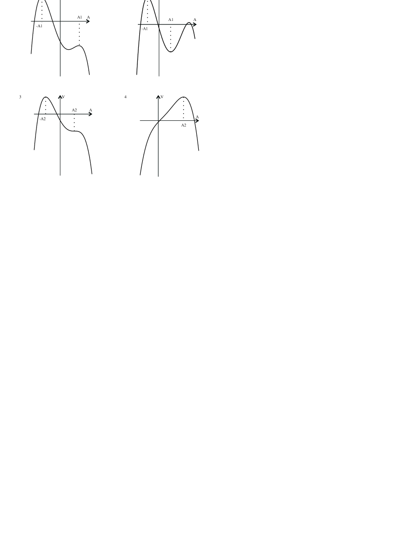
Figure 8.1: A sketch of the effective potential $V(A)=\lambda A+\frac{1}{3}gA^{3}-\frac{1}{4}(gA^{2}+\lambda)^{2}$ for the four different cases discussed in the text. Here $A_{1}=\sqrt{-\lambda/g}$ and $A_{2}=1/g$.

• Suppose $\sqrt{-\lambda g}>1$. In this case $V^{\prime\prime}(A)<0$ for both the roots $A=\pm\sqrt{-\lambda/g}$, hence $U^{\prime\prime}(A)=2$ must correspond to the local minimum. Thus for this vacuum solution supersymmetry will be broken (see Fig. 8.1a).

• Suppose $0<\sqrt{-\lambda g}<1$. In this case one of the roots $A=\pm\sqrt{-\lambda/g}$ will correspond to a local maximum the other to a local minimum. Thus there exists a supersymmetry preserving vacuum solution (see Fig. 8.1b).

• Suppose $-\lambda g=1$. Then $A=\pm\sqrt{-\lambda/g}=\pm 1/g$ implies that one of the two roots corresponds to $V^{\prime\prime}(A)=0$, the other to a maximum. Thus there exists no stable supersymmetry preserving vacuum state (see Fig. 8.1c).

• Suppose $\lambda g>0$. There is no solution to $U^{\prime}(A)=0$, hence supersymmetry will be broken. However, in this case $V(A)$ has a single maximum at $A=1/g$ and thus any vacuum solution will be unstable anyway (see Fig. 8.1d).

Note, however, that the effective potential of Eqn. (8.7) is unbounded from below and as such exhibits only local minima. Therefore there do not exist true vacuum solutions.

9 Conserved currents from superfield formalism

Using the superfield formalism we will derive in this section a supersymmetric generalization of the energy-momentum tensor.

In order to do so consider some superfield Lagrangian density $\mathcal{L}=\mathcal{L}(\Phi,\partial\Phi)$. Remember that a coordinate transformation $X^{M}\rightarrow X^{M}+\delta X^{M}$ is realized on superscalar fields as (see Eqn. (4.11)) $\Phi\rightarrow\Phi(X-\delta X)=\Phi(X)+\delta\Phi(X)$ where $\delta\Phi=-\delta X^{M}\partial_{M}\Phi$. Note that in the case of an isometry, as we shall assume here, we have $\delta X^{M}=\delta uK^{M}$, with $K^{M}$ a Killing supervector.

Similarly we find that the Lagrangian density transforms under an isometry as

$$\delta\mathcal{L}=-(-1)^{M}\partial_{M}\left(\delta X^{M}\mathcal{L}\right).$$ (9.1)

For a derivation of this result see Appendix A.6. On the other hand we find that the change in the Lagrangian density obtained by varying the fields is

$$\delta\mathcal{L} =\delta\Phi\frac{\partial\mathcal{L}}{\partial\Phi}+\left(\partial_{M}\delta\Phi\right)\frac{\partial\mathcal{L}}{\partial(\partial_{M}\Phi)}$$

$$=\delta\Phi\left(\frac{\partial\mathcal{L}}{\partial\Phi}-\partial_{M}\left(\frac{\partial\mathcal{L}}{\partial(\partial_{M}\Phi)}\right)\right)+\partial_{M}\left(\delta\Phi\frac{\partial\mathcal{L}}{\partial(\partial_{M}\Phi)}\right).$$ (9.2)

From this we see that the Euler-Lagrange equations are

$$\frac{\partial\mathcal{L}}{\partial\Phi}-\partial_{M}\left(\frac{\partial\mathcal{L}}{\partial(\partial_{M}\Phi)}\right)=0.$$ (9.3)

Thus if we impose the field equations the first term in Eqn. (9.2) vanishes and we can set the remaining term equal to $-(-1)^{M}\partial_{M}\left(\delta X^{M}\mathcal{L}\right)$. Then using $\delta\Phi=-\delta X^{M}\partial_{M}\Phi$ we find

$$\partial_{M}\left(\delta X^{N}\left((-1)^{M}\delta_{N}{}^{M}\mathcal{L}-\partial_{N}\Phi\frac{\partial\mathcal{L}}{\partial(\partial_{M}\Phi)}\right)\right)=0.$$ (9.4)

We are now in the position to define the super energy-momentum tensor $\mathcal{T}_{N}{}^{M}$

$$\mathcal{T}_{N}{}^{M}=(-1)^{M}\delta_{N}{}^{M}\mathcal{L}-\partial_{N}\Phi\frac{\partial\mathcal{L}}{\partial(\partial_{M}\Phi)}.$$ (9.5)

The corresponding super Noether current $\mathcal{J}^{M}$ is then defined by

$$\mathcal{J}^{M}=K^{N}\mathcal{T}_{N}{}^{M}.$$ (9.6)

By means of Eqn. (9.4) $\mathcal{J}^{M}$ will satisfy the super conservation law

$$\partial_{M}\mathcal{J}^{M}=0.$$ (9.7)

Let us now consider the specific Lagrangian density for $S^{2|2}$ given by (see Eqns. (7.7, 7.33))

$$\mathcal{L}=E\left(E_{-}\Phi E_{+}\Phi+\frac{1}{4}U(\Phi)\right).$$ (9.8)

One can check that the field equations given by Eqn. (9.3) indeed coincide — when written in terms of the component fields — with the field equations given in Appendix A.4, which were directly derived from the action in terms of the component fields.

For the super energy-momentum tensor we find in this case

$$\begin{split}\mathcal{T}_{N}{}^{M}&=(-1)^{M}\delta_{N}{}^{M}E\left(E_{-}\Phi E_{+}\Phi+\frac{1}{4}U(\Phi)\right)\\ &\hskip 12.91663pt-\partial_{N}\Phi E\left(E_{-}{}^{M}E_{+}\Phi+(-1)^{M}E_{-}\Phi E_{+}{}^{M}\right).\end{split}$$ (9.9)

The supercurrents are given by

$$\mathcal{J}_{p}{}^{M}=K_{p}{}^{N}\mathcal{T}_{N}{}^{M},$$ (9.10)

with $p=0,1,2,-,+$, as before. The Killing supervectors $K_{p}{}^{N}$ can be read off from Eqns. (4.14–4.18). Note that by taking the $\chi\chi^{\diamond}$ component of the conservation equation, Eqn. (9.7), we find a conservation equation purely in $z$

$$\left(\partial_{M}\mathcal{J}_{p}{}^{M}\right){\Big{|}}_{\chi\chi^{\diamond}}=(\partial_{z}\mathcal{J}_{p}{}^{z}+\partial_{z^{\diamond}}\mathcal{J}_{p}{}^{z^{\diamond}}){\Big{|}}_{\chi\chi^{\diamond}}=(\partial_{m}\mathcal{J}_{p}{}^{m}){\Big{|}}_{\chi\chi^{\diamond}}=0,$$ (9.11)

as both $\partial_{\chi}\mathcal{J}_{p}{}^{\chi}$ and $\partial_{\chi^{\diamond}}\mathcal{J}_{p}{}^{\chi^{\diamond}}$ do not contribute a $\chi\chi^{\diamond}$ term. It will turn out that it is this $\chi\chi^{\diamond}$ contribution to the conservation equation that gives rise to the familiar energy-momentum tensor and fermionic currents, which can alternatively be derived directly from the action in terms of the component fields. Considering other components of the conservation equation, say the $\chi$ component, we find

$$(\partial_{z}\mathcal{J}_{p}{}^{z}+\partial_{z^{\diamond}}\mathcal{J}_{p}{}^{z^{\diamond}}){\Big{|}}_{\chi} =-(\partial_{\chi^{\diamond}}\mathcal{J}_{p}{}^{\chi^{\diamond}}){\Big{|}}_{\chi}.$$ (9.12)

Note that this also is a conservation equation purely in $z$. However, the term on the right hand side of the equation, $-(\partial_{\chi^{\diamond}}\mathcal{J}_{p}{}^{\chi^{\diamond}}){\big{|}}_{\chi}$, which does not involve any derivatives with respect to $z$, must be understood as some kind of source term. Yet, the interpretation of these additional conservation equations remains unclear.

Now let us consider the currents $\mathcal{J}_{i}{}^{m}$, $i=0,1,2$, in more detail. We have

$$\mathcal{J}_{i}{}^{m}=K_{i}{}^{N}\mathcal{T}_{N}{}^{m}=K_{i}{}^{n}\mathcal{T}_{n}{}^{m}+K_{i}{}^{\mu}\mathcal{T}_{\mu}{}^{m}.$$

By direct calculation one finds that the components $\mathcal{T}_{\chi}{}^{m}$ are proportional to $\chi$ and similarly the components $\mathcal{T}_{\chi^{\diamond}}{}^{m}$ are proportional to $\chi^{\diamond}$. Now, as also $K_{i}{}^{\chi}$ is proportional to $\chi$ and similarly $K_{i}{}^{\chi^{\diamond}}$ is proportional to $\chi^{\diamond}$ the above equation simplifies to

$$\mathcal{J}_{i}{}^{m}=K_{i}{}^{n}\mathcal{T}_{n}{}^{m}.$$ (9.13)

Note that $K_{i}{}^{n}=K_{i}{}^{n}{\big{|}}_{\chi\chi^{\diamond}}\equiv k_{i}{}^{n}$ correspond to the usual Killing vectors on the sphere $S^{2|0}$

$$(k_{0}^{m}) =i\left(z,-z^{\diamond}\right),$$ (9.14)

$$(k_{1}^{m}) =\frac{i}{2}\left((1-z^{2}),-(1-{z^{\diamond}}^{2})\right),$$ (9.15)

$$(k_{2}^{m}) =-\frac{1}{2}\left((1+z^{2}),(1+{z^{\diamond}}^{2})\right).$$ (9.16)

Defining $j_{i}{}^{m}$ and $t_{m}{}^{n}$ as the $\chi\chi^{\diamond}$ components of $\mathcal{J}_{i}{}^{m}$ and $\mathcal{T}_{m}{}^{n}$, respectively

$$j_{i}{}^{m}\equiv\mathcal{J}_{i}{}^{m}{\Big{|}}_{\chi\chi^{\diamond}},\qquad t_{m}{}^{n}\equiv\mathcal{T}_{m}{}^{n}{\Big{|}}_{\chi\chi^{\diamond}}$$

we can rewrite the conservation equation, Eqn. (9.11), for the bosonic currents $\mathcal{J}_{i}{}^{m}$ as

$$\partial_{m}j_{i}{}^{m}=\partial_{m}(k_{i}{}^{n}t_{n}{}^{m})=0.$$ (9.17)

For $t_{m}{}^{n}$ we find in terms of the conformally rescaled fields $\tilde{A}$, $\psi_{-}$, $\psi_{+}$, as given in Eqns. (6.24–6.26),

$$\begin{split}t_{mn}&=\frac{i}{8}\sqrt{|g|}\bigg{(}\partial_{m}\tilde{A}\partial_{n}\tilde{A}+\frac{i}{2}\psi^{\ddagger}\gamma_{m}\partial_{n}\psi\\ &\hskip 43.05542pt-g_{mn}\left[\frac{1}{2}(\partial\tilde{A})^{2}-\frac{1}{8}U^{\prime}(\tilde{A})^{2}+\frac{1}{2}U(\tilde{A})\right]\bigg{)},\end{split}$$ (9.18)

where the index has been lowered using the metric $g_{mn}$. Note that the auxiliary field $\tilde{F}$ has been eliminated.

We shall now consider the $\chi\chi^{\diamond}$ contribution to the currents $\mathcal{J}_{\alpha}{}^{m}$, $\alpha=-,+$. Let us define

$$j_{\alpha}{}^{m}\equiv\mathcal{J}_{\alpha}{}^{m}\Big{|}_{\chi\chi^{\diamond}}$$ (9.19)

and also

$$j^{m}\equiv\beta^{\diamond}j_{-}{}^{m}+\beta j_{+}{}^{m}.$$ (9.20)

From Eqn. (9.11) we see that $j^{m}$ satisfies the conservation equation

$$\partial_{m}j^{m}=0.$$ (9.21)

Rewriting this fermionic current in terms of the rescaled fields $\tilde{A}$, $\psi_{-}$, $\psi_{+}$, as we did before in the case of $t_{nm}$, we find

$$j^{m}=\frac{i}{8}\sqrt{|g|}\boldsymbol{\epsilon}^{\ddagger}\left(\partial\!\!\!/\tilde{A}+\frac{i}{2}U^{\prime}(\tilde{A})\right)\gamma^{m}\boldsymbol{\psi},$$ (9.22)

where $\boldsymbol{\epsilon}$ is the Killing spinor defined in Eqn. (6.19).

10 Conclusions and Outlook

We have shown how to construct the supersphere $S^{2|2}$ as the coset space $U\!O\!Sp(1|2)/\mathcal{U}(1)$, analogous to the construction of flat superspace as the super Poincaré group quotiented by the Lorentz group. The definition of $U\!O\!Sp(1|2)$, which is the isometry group of the supersphere, required the notions of pseudo-conjugation and graded adjoint.

The coset space $U\!O\!Sp(1|2)/\mathcal{U}(1)$ has the structure of a superspace, rather than just being a supermanifold as is the case for other coset space definitions of the supersphere. This allowed us to consider the supersphere as a base space for a superscalar field theory. As $S^{2|2}$ is an example of a curved superspace on which we have rigid supersymmetry transformations, i.e. the supersymmetry parameter is not position dependent, the theory we constructed exhibits global supersymmetry. Upon integrating out the odd coordinate dependence, this superscalar field theory becomes a supersymmetric theory on the ordinary sphere with a scalar, spinor and auxiliary field. Choosing a polynomial potential we saw that solutions at local minima may break supersymmetry, provided certain conditions are met. Also recall that, contrary to what is expected, the effective potential for this model is not typically bounded from below. This appears to be due to the Euclidean nature of the theory. However, as we pointed out, non-polynomial potentials can be found which will exhibit global minima and thus true vacuum solutions.

Using the superfield formalism we were able to derive Euler-Lagrange equations and Noether’s theorem for the superscalar field $\Phi$ itself, starting from some general superfield Lagrangian density $\mathcal{L}(\Phi,\partial\Phi)$. When applying Euler-Lagrange equations to the specific Lagrangian density constructed for $S^{2|2}$ we found that the field equations for $\Phi$ reduce, when written in terms of the component fields, to the ones derived directly from the action on the ordinary sphere. The super conservation equations derived from Noether’s theorem — when applied to the Lagrangian density for the supersphere — give rise to the familiar energy-momentum tensor and fermionic currents expected from the component field action. Notably, though, the super conservation equations also give rise to additional conservation laws, that appear to be independent of the familiar ones and which thus call for some interpretation.

In this work we have concentrated on superscalar field theories on the supersphere. Using the methods we have presented it would be possible to further this study by investigating more general field theories, for example gauge theories or sigma models with the supersphere as the base space. Another possible extension of this work would be to quantize the scalar field theory, which due to its Euclidean nature would correspond to a statistical field theory.

Appendix A Appendix

A.1 Raising and lowering conventions for spinor indices

Raising and lowering of spinor indices $\alpha,\beta,\ldots$ is achieved with the use of the antisymmetric epsilon symbols $\epsilon^{\alpha\beta}$ and $\epsilon_{\alpha\beta}$; the convention we will follow is that of [14]. When raising an index we always contract on the second index of $\epsilon^{\alpha\beta}$, e.g.

$$\psi^{\alpha}=\epsilon^{\alpha\beta}\psi_{\beta}.$$ (A.1)

However, when lowering an index we always contract on the first index of $\epsilon_{\alpha\beta}$, e.g.

$$\psi_{\beta}=\epsilon_{\gamma\beta}\psi^{\gamma}.$$ (A.2)

Combining the previous two equations we see that

$$\epsilon^{\alpha\beta}\epsilon_{\gamma\beta}=\delta^{\alpha}{}_{\gamma}.$$ (A.3)

Hence we see that if we choose $\epsilon_{-+}=1$, then we must also have $\epsilon^{-+}=1$. Note that we can think of $\epsilon^{\alpha\beta}$ as $\epsilon_{\alpha\beta}$ with both indices raised.

The (components of the) standard Pauli matrices are taken to be $(\sigma^{i})^{\alpha}{}_{\beta}$. Lowering the first index allows us to construct the quantity

$$(\sigma^{i})_{\alpha\beta}=\epsilon_{\gamma\alpha}(\sigma^{i})^{\gamma}{}_{\beta}=-\epsilon_{\alpha\gamma}(\sigma^{i})^{\gamma}{}_{\beta},$$ (A.4)

which is symmetric in $\alpha,\beta$. We can then raise the second index to give

$$(\sigma^{i})_{\alpha}{}^{\beta}=\epsilon_{\gamma\alpha}(\sigma^{i})^{\gamma}{}_{\delta}\epsilon^{\beta\delta}=\epsilon_{\alpha\gamma}(\sigma^{i})^{\gamma}{}_{\delta}\epsilon^{\delta\beta}.$$ (A.5)

Notice that the third terms in Eqns. (A.4, A.5) have been written in a way more suggestive of standard matrix multiplication. In fact, if we define the antisymmetric matrix $\epsilon=(\epsilon_{\alpha\beta})$, we may think of these quantities as the components of the matrices $-\epsilon\sigma^{i}$ and $\epsilon\sigma^{i}\epsilon=(\sigma^{i})^{\mathrm{t}}$ respectively.

The quantity $(\sigma^{i})_{\alpha}{}^{\beta}$ (as well as $(\sigma^{a})_{\alpha}{}^{\beta}$) is a $\mathcal{U}(1)$ invariant tensor, i.e.

$$(\sigma^{i})_{\alpha}{}^{\beta}=R_{\alpha}{}^{\gamma}(h)(\sigma^{j})_{\gamma}{}^{\delta}R_{\delta}{}^{\beta}(h^{-1})R_{j}{}^{i}(h^{-1}),$$ (A.6)

where $R_{p}{}^{q}(h)$ is as given in Eqn. (5.13).

A.2 Superzweibein and spin connection in polar coordinates

We obtain for the superzweibein in (super)-polar coordinates

$$(\tilde{E}_{M}{}^{A})={\mbox{\scriptsize$\left(\!\begin{array}[]{cc|cc}\sin\!\theta&0&0&0\\ 0&-1&0&0\\ \hline\cr\frac{i}{4}(\eta^{\diamond}\sin\!\theta-\eta\cos\!\theta e^{-i\varphi})&-\frac{1}{4}\eta e^{-i\varphi}&(1+\frac{1}{8}\eta\eta^{\diamond})\sin\!\frac{\theta}{2}e^{-i\varphi/2}&(1+\frac{1}{8}\eta\eta^{\diamond})\cos\!\frac{\theta}{2}e^{-i\varphi/2}\\ \frac{i}{4}(\eta\sin\!\theta+\eta^{\diamond}\cos\!\theta e^{i\varphi})&-\frac{1}{4}\eta^{\diamond}e^{i\varphi}&(1+\frac{1}{8}\eta\eta^{\diamond})\cos\!\frac{\theta}{2}e^{i\varphi/2}&-(1+\frac{1}{8}\eta\eta^{\diamond})\sin\!\frac{\theta}{2}e^{i\varphi/2}\end{array}\!\right)$}},$$ (A.7)

where the index $M$ here runs over $\varphi,\theta,\eta,\eta^{\diamond}$. The spin connection is in polar coordinates given by

$$\omega^{0} =-d\varphi\cos\!\theta-\frac{i}{4}d\eta^{\diamond}(\eta\cos\!\theta-\eta^{\diamond}e^{i\varphi}\sin\!\theta)-\frac{i}{4}d\eta(\eta^{\diamond}\cos\!\theta+\eta e^{-i\varphi}\sin\!\theta)$$ (A.8)

$$=-\cot\!\theta\tilde{E}^{1}+\frac{i}{4}\frac{1}{\sin\!\theta}(\eta e^{-i\varphi/2}\sin\!\frac{\theta}{2}-\eta^{\diamond}e^{i\varphi/2}\cos\!\frac{\theta}{2})\tilde{E}^{-}$$

$${}\hskip 53.81927pt+\frac{i}{4}\frac{1}{\sin\!\theta}(\eta e^{-i\varphi/2}\cos\!\frac{\theta}{2}+\eta^{\diamond}e^{i\varphi/2}\sin\!\frac{\theta}{2})\tilde{E}^{+}.$$ (A.9)

A.3 Superzweibein and spin connection in the $(w,\zeta)$ patch

We find for the superzweibein in the $(w,\zeta)$ coordinate patch

$$(E^{\prime}_{M}{}^{A})=\left(\!\begin{array}[]{cc|cc}\frac{i}{1+ww^{\diamond}+\zeta\zeta^{\diamond}}&\frac{-1}{1+ww^{\diamond}+\zeta\zeta^{\diamond}}&\frac{2i(\zeta w^{\diamond}+\zeta^{\diamond})}{(1+ww^{\diamond})^{3/2}}&0\\ \frac{-i}{1+ww^{\diamond}+\zeta\zeta^{\diamond}}&\frac{-1}{1+ww^{\diamond}+\zeta\zeta^{\diamond}}&0&\frac{2i(\zeta^{\diamond}w-\zeta)}{(1+ww^{\diamond})^{3/2}}\\ \hline\cr\frac{-i\zeta}{1+ww^{\diamond}}&\frac{\zeta}{1+ww^{\diamond}}&\frac{-2i}{(1+ww^{\diamond}-\zeta\zeta^{\diamond})^{1/2}}&0\\ \frac{i\zeta^{\diamond}}{1+ww^{\diamond}}&\frac{\zeta^{\diamond}}{1+ww^{\diamond}}&0&\frac{-2i}{(1+ww^{\diamond}-\zeta\zeta^{\diamond})^{1/2}}\\ \end{array}\!\right),$$ (A.10)

where the index $M$ now runs over $w,w^{\diamond},\zeta,\zeta^{\diamond}$. The inverse superzweibein is given by

$$(E^{\prime}_{A}{}^{M})={\mbox{\scriptsize$\left(\!\begin{array}[]{cc|cc}-\frac{i}{2}(1+ww^{\diamond})&\frac{i}{2}(1+ww^{\diamond})&-\frac{i}{2}(\zeta w^{\diamond}+\zeta^{\diamond})&\frac{i}{2}(\zeta^{\diamond}w-\zeta)\\ -\frac{1}{2}(1+ww^{\diamond})&-\frac{1}{2}(1+ww^{\diamond})&-\frac{1}{2}(\zeta w^{\diamond}+\zeta^{\diamond})&-\frac{1}{2}(\zeta^{\diamond}w-\zeta)\\ \hline\cr\frac{i}{2}(1+ww^{\diamond})^{1/2}\zeta&0&\frac{i}{2}(1+ww^{\diamond}+\zeta\zeta^{\diamond})^{1/2}&0\\ 0&\frac{i}{2}(1+ww^{\diamond})^{1/2}\zeta^{\diamond}&0&\frac{i}{2}(1+ww^{\diamond}+\zeta\zeta^{\diamond})^{1/2}\\ \end{array}\!\right)$}}.$$ (A.11)

The superdeterminant of $(E^{\prime}_{M}{}^{A})$ is given by

$$E^{\prime}\equiv\mathrm{sdet}(E^{\prime}_{M}{}^{A})=\frac{i}{2}\;\frac{1}{1+ww^{\diamond}+\zeta\zeta^{\diamond}}.$$ (A.12)

Finally, we find for the spin connection in the $(w,\zeta)$ coordinate patch

$$\omega^{\prime 0} =\frac{i}{1+ww^{\diamond}+\zeta\zeta^{\diamond}}(w^{\diamond}dw-wdw^{\diamond}+d\zeta\zeta^{\diamond}+d\zeta^{\diamond}\zeta)$$ (A.13)

$$=\frac{1}{2}(w^{\diamond}+w)E^{\prime 1}-\frac{i}{2}(w^{\diamond}-w)E^{\prime 2}$$

$$\hskip 10.76385pt+\frac{1}{2}\frac{\zeta w^{\diamond}+\zeta^{\diamond}}{(1+ww^{\diamond})^{1/2}}E^{\prime-}-\frac{1}{2}\frac{\zeta^{\diamond}w-\zeta}{(1+ww^{\diamond})^{1/2}}E^{\prime+}.$$ (A.14)

A.4 Euler-Lagrange equations for the full action

The field equations following from the full action given in Eqn. (LABEL:eqn:fullaction) are

$$\partial_{z}\partial_{z^{\diamond}}A =\frac{1}{2}\frac{U^{\prime}(A)}{(1+zz^{\diamond})^{2}}-\frac{1}{2}\frac{FU^{\prime\prime}(A)}{1+zz^{\diamond}}+\frac{1}{2}\frac{\psi_{\chi}\psi_{\chi^{\diamond}}U^{\prime\prime\prime}(A)}{1+zz^{\diamond}}$$ (A.15)

$$\partial_{z^{\diamond}}\psi_{\chi} =-\frac{1}{2}\frac{\psi_{\chi^{\diamond}}U^{\prime\prime}(A)}{1+zz^{\diamond}}$$ (A.16)

$$\partial_{z}\psi_{\chi^{\diamond}} =\frac{1}{2}\frac{\psi_{\chi}U^{\prime\prime}(A)}{1+zz^{\diamond}}$$ (A.17)

$$F =\frac{1}{2}\frac{U^{\prime}(A)}{1+zz^{\diamond}}.$$ (A.18)

A.5 Conformal invariance of the kinetic part of the action

The superscalar field action, Eqn. (LABEL:eqn:fullaction), can be rewritten using the notation of Section 6.2. We find it to be

$$I =\frac{i}{16}\int d^{2}z\;\sqrt{|g|}\bigg{(}g^{mn}\partial_{m}\tilde{A}\partial_{n}\tilde{A}+i\boldsymbol{\psi}^{\ddagger}\partial\!\!\!/\boldsymbol{\psi}+\tilde{F}^{2}$$

$$\hskip 64.58313pt-\frac{1}{2}\boldsymbol{\psi}^{\ddagger}\boldsymbol{\psi}U^{\prime\prime}(\tilde{A})+U(\tilde{A})+\tilde{F}U^{\prime}(\tilde{A})\bigg{)},$$ (A.19)

where $g$ is the determinant of the metric. The kinetic part of the action is obtained by setting $U(\tilde{A})=0$. Note that we could replace the second term, $i\boldsymbol{\psi}^{\ddagger}\partial\!\!\!/\boldsymbol{\psi}$, with $i\boldsymbol{\psi}^{\ddagger}D\!\!\!\!/\boldsymbol{\psi}$. This is because the term involving the spin connection will vanish due to the anticommuting nature of $\boldsymbol{\psi}$ and the form of the gamma matrices.

Under a conformal transformation, the metric and gamma matrices transform as

$$g_{mn} \to\lambda^{2}g_{mn}$$ (A.20)

$$\gamma^{m} \to\lambda^{-1}\gamma^{m}$$ (A.21)

where $\lambda$ is some positive function on the sphere. It is then possible to define the transformation properties of the component fields in such a way that the kinetic part of the action will remain invariant. We find

$$\tilde{A} \to\tilde{A},$$ (A.22)

$$\boldsymbol{\psi} \to\lambda^{-\frac{1}{2}}\boldsymbol{\psi},$$ (A.23)

$$\tilde{F} \to\lambda^{-1}\tilde{F}.$$ (A.24)

The presence of a non-zero potential will break this conformal invariance.

A.6 Transformation properties of superscalar densities

Using the infinitesimal point transformation $X^{\prime M}=X^{M}+\delta u\,\Xi^{M}(X)$ we can define the Lie derivative of any supertensor field $T(X)$ by

$${}_{\Xi}T(X)=\lim_{\delta u\to 0}\frac{T(X^{\prime})-T^{\prime}(X^{\prime})}{\delta u}.$$ (A.25)

For instance, a superscalar transforms as $\Phi^{\prime}(X^{\prime})=\Phi(X)$, hence the Lie derivative can be calculated by using a Taylor expansion. We find

$${}_{\Xi}\Phi(X)=\Xi^{M}\partial_{M}\Phi(X).$$ (A.26)

Now, let $\mathfrak{T}(X)$ be a superscalar density of weight $+1$. It is defined to transform as

$$\mathfrak{T}^{\prime}(X^{\prime})=J(X)\mathfrak{T}(X),$$ (A.27)

where $J(X)$ is given by the superdeterminant

$$J(X) =\mathrm{sdet}\left(\frac{\partial X^{M}}{\partial X^{\prime N}}\right)$$ (A.28)

$$=1-\delta u(-1)^{M}\partial_{M}\Xi^{M}+\ldots$$ (A.29)

Note that in the last line we have expanded the superdeterminant to first order, resulting in the appearance of a supertrace, this explains the factor $(-1)^{M}$ in the summation over $M$. Also we can expand

$$\mathfrak{T}(X^{\prime})=\mathfrak{T}(X)+\delta u\,\Xi^{M}\partial_{M}\mathfrak{T}(X)+\ldots$$ (A.30)

Combining these gives us the Lie derivative of a superscalar density

$${}_{\Xi}\mathfrak{T}(X)=(-1)^{M}\partial_{M}(\Xi^{M}\mathfrak{T}(X)).$$ (A.31)

The same procedure can be used to calculate the Lie derivative of any supertensor field.

Using the Lie derivative we can describe the infinitesimal active coordinate transformation, $X\to X+\delta u\,\Xi$, alternatively as a transformation of the fields. We need to find the difference between the tensor which has been dragged along $\delta u\,\Xi$ to the point $X$, and the tensor which was already at $X$. For the supertensor field $T(X)$ this difference is given by

$$\delta T(X)=-\delta u_{\Xi}T(X).$$ (A.32)

References

- [1] J. A. de Azcárraga, J. M. Izquierdo, and W. J. Zakrzewski, “A supergroup based supersigma model,” J. Math. Phys. 33 (1992) 2357–2364.
- [2] N. Read and H. Saleur, “Exact spectra of conformal supersymmetric nonlinear sigma models in two dimensions,” Nucl. Phys. B613 (2001) 409–444, hep-th/0106124.
- [3] G. Landi, “Projective Modules of Finite Type over the Supersphere ,” Diff. Geom. Appl. 14 (2001) 95–111, math-ph/9907020.
- [4] G. Landi and G. Marmo, “Extensions of Lie Superalgebras and Supersymmetric Abelian Gauge Fields,” Phys. Lett. B193 (1987) 61–66.
- [5] E. Ivanov, L. Mezincescu, and P. K. Townsend, “Fuzzy as a quantum superspace,” (2003) hep-th/0311159.
- [6] V. Rittenberg and V. Scheunert, “Elementary construction of graded Lie groups,” J. Math. Phys. 19 (1978) 709–713.
- [7] W. A. Bardeen and D. Z. Freedman, “On the energy crisis in anti-de Sitter supersymmetry,” Nuclear Physics B 253 (1985) 635–649.
- [8] B. DeWitt, Supermanifolds. Cambridge Monographs on Mathematical Physics. Cambridge University Press, 1984.
- [9] I. L. Buchbinder and S. M. Kuzenko, Ideas and Methods of Supersymmetry and Supergravity. Institute of Physics Publishing, 1995.
- [10] P. West, Introduction to Supersymmetry and Supergravity. World Scientific, 1990.
- [11] N. Alonso-Alberca, E. Lozano-Tellechea, and T. Ort n, “Geometric Construction of Killing Spinors and Supersymmetry Algebras in Homogeneous Spacetimes,” Class. Quant. Grav. 19 (2002) 6009–6024, hep-th/0208158.
- [12] N. Dragon, “Torsion and Curvature in Extended Supergravity,” Z. Phys. C2 (1979) 29–32.
- [13] Y. Fuji and K. Yamagishi, “Killing spinors on spheres and hyperbolic manifolds,” J. Math. Phys. 27 (1986) 979–981.
- [14] R. Penrose and W. Rindler, Spinors and space-time, Volume 1: Two-spinor calculus and relativistic fields. Cambridge University Press, 1984.