CERN-PH-TH/2004-189

Non-perturbative vacua for M-theory on $G_{2}$ manifolds

We study moduli stabilization in the context of M-theory on compact manifolds with $G_{2}$ holonomy, using superpotentials from flux and membrane instantons, and recent results for the Kähler potential of such models. The existence of minima with negative cosmological constant, stabilizing all moduli, is established. While most of these minima preserve supersymmetry, we also find examples with broken supersymmetry. Supersymmetric vacua with vanishing cosmological constant can also be obtained after a suitable tuning of parameters.

1 Introduction

The stabilization of moduli is a long-standing problem in string theory. Traditionally, attempts to solve it have included non-perturbative effects, such as gaugino condensation, that generate a (super)-potential for the moduli fields. There is a substantial body of literature on this subject, particularly in the context of heterotic string theory, see for example [1]–[18]. It is fairly difficult to find models with proper minima in this way, and it is probably fair to say that successful models constructed along these lines usually require special parameter choices and some degree of tuning [6]. The resulting minima are quite shallow and only separated from runaway directions by a small barrier [19, 20]. These problems can be traced back to the nature of non-perturbative superpotentials, which are double-exponential in (canonically normalized) moduli fields.

Recently, progress has been made by using flux of anti-symmetric tensor fields to stabilize moduli [21]. Unlike non-perturbative superpotentials, superpotentials from flux are merely single-exponential in canonically normalized moduli fields and are, therefore, more likely to produce minima. It has been known for some time [3, 22, 23, 24, 25] that a combination of flux and non-perturbative effects can stabilize moduli successfully, and under relatively generic conditions, but only with recent advances in the understanding of flux compactifications [26]–[38] has this possibility been analyzed more systematically [39]–[41]. In this paper we will present the first systematic analysis of this problem for M-theory on manifolds of $G_{2}$ holonomy with a superpotential from flux and membrane instantons.

M-theory on (compact) manifolds $X$ of $G_{2}$ holonomy leads to non-chiral [42] four-dimensional effective theories with $N=1$ supersymmetry [43, 44]. Non-Abelian gauge groups and matter fields, which may account for the standard model particles, arise when the $G_{2}$ space develops singularities [45]–[53]. In this paper we will not consider such possible matter field sectors, but focus on the gravity/moduli part of the theory, which contains $b^{3}(X)$ chiral moduli multiplets $\Phi^{I}$. Their real parts parameterize the moduli space of the $G_{2}$ manifold, while their imaginary parts corresponds to axions. We are interested in stabilizing these moduli fields $\Phi^{I}$, combining the effects of flux and membrane instantons. The flux superpotential has been computed in Ref. [27, 44], while the result for the structure of membrane instanton contributions to the superpotential can be found in Ref. [54]. The scalar potential of four-dimensional $N=1$ supergravity also depends on the Kähler potential for which we rely on the results of Ref. [55]. We will be focusing on compact $G_{2}$ manifolds constructed by blowing up the singularities of $G_{2}$ orbifolds [56, 57, 58, 45]. For such $G_{2}$ manifolds, the moduli naturally split into two classes, $(\Phi^{I})=(T^{a},U^{i})$, namely the “bulk” moduli $T^{a}$ associated with the underlying torus and the “blow-up” moduli $U^{i}$ that arise from blowing up the singularities. We will address the stabilization of both types of moduli for realistic models.

A practical problem is that there are no simple compact $G_{2}$ manifolds with, say, $b^{3}(X)=1$ available. In particular, the calculation of the Kähler potential in Ref. [55] has been carried out for an example with $b^{3}(X)=43$. We will, therefore, have to deal with a large number of moduli. This task will be approached by starting with relatively simple, but characteristic, toy models and then working our way up to include the full complications of more realistic cases. After setting up the structure of the models in the next section, Section 3 discusses the stabilization of the bulk moduli $T^{a}$, first for a simple universal case, and then including all bulk moduli. Section 4 includes the blow-up moduli $U^{i}$, again starting with a simple universal toy model and then moving on to include all moduli. Conclusions and further directions are presented in Section 5.

2 General structure of four-dimensional effective theories

In this section, we will review the structure of four-dimensional $N=1$ theories, which originate from M-theory on (compact) $G_{2}$ manifolds. These four-dimensional models will form the basis for the subsequent analysis in this paper. For mathematical facts on manifolds with $G_{2}$ holonomy we refer to Ref. [58]. Many of the physics aspects of the following presentation can be found in Refs. [43, 44].

Before we specialize to the models considered in this paper, let us collect a number of useful general facts about M-theory on $G_{2}$ manifolds. A seven-dimensional manifold $X$ with holonomy $G_{2}$ has a vanishing first Betti number, $b^{1}(X)=0$, and its cohomology is, therefore, characterized by $b^{2}(X)$ and $b^{3}(X)$. When compactifying M-theory on such a manifold, the resulting four-dimensional low-energy theory has $N=1$ supersymmetry and contains $b^{2}(X)$ Abelian vector multiplets and $b^{3}(X)$ uncharged chiral multiplets [42, 43]. We denote these latter chiral fields, which are the primary focus of this paper, by $\Phi^{I}$, $I,J,\dots=1,\dots,b^{3}(X)$.

To compute the scalar potential we will need an explicit expression for the Kähler potential of these chiral superfields. Ideally, one would like a generic and explicit formulae that may depend on topological data of the $G_{2}$ manifold in question, but still applies to all $G_{2}$ manifolds. Unfortunately, no such formula is known. We will go around this problem by focusing on a particular class of $G_{2}$ manifold for which an (approximate) form of the Kähler potential is known. However, let us first collect some general facts. It is known [44] that the Kähler potential can be expressed in terms of the volume ${\cal V}$ of the internal manifold as

$$K=-3\ln\left(\frac{{\cal V}}{2\pi^{2}}\right)\;.$$ (2.1)

This relation implies that $K$ only depends on geometrical data and is, hence, independent of the axionic fields, which we take to be the imaginary parts of the chiral fields $\Phi^{I}$. We, therefore, have

$$K=K(\Phi^{I}+\bar{\Phi}^{I})\;.$$ (2.2)

Further, it can be shown [44] that a rescaling of the $G_{2}$ space by a factor $\lambda$, corresponding to a change ${\cal V}\rightarrow\lambda^{7}{\cal V}$ of the volume, leads to a scaling $(\Phi^{I}+\bar{\Phi}^{I})\rightarrow\lambda^{3}(\Phi^{I}+\bar{\Phi}^{I})$. Hence, the real parts of the chiral fields $\Phi^{I}$ measure three-dimensional volumes. More precisely, they are proportional to the volumes of (a basis of) three cycles of the $G_{2}$ manifold.

It can be shown by straightforward dimensional reduction [55, 43] that the gauge kinetic functions $f$ of the gauge multiplets are of the form

$$f=c_{I}\Phi^{I}\;,$$ (2.3)

where $c_{I}$ are constant coefficients that depend on the $G_{2}$ manifold and the gauge multiplet under consideration.

Perturbatively, and in the absence of flux, the superpotential $W$ vanishes. It has been shown [27, 44] that internal flux of the M-theory four-form field strength leads to a superpotential

$$W_{\rm flux}=m_{I}\Phi^{I}\;,$$ (2.4)

where the flux parameters $m_{I}$ are quantized. Non-perturbatively, an additional contribution to the superpotential is generated by membrane instantons [54] wrapping three-cycles within the $G_{2}$ manifold. A typical instanton superpotential is given by a sum of terms of the form

$$W_{\rm inst}\sim\exp(-p_{I}\Phi^{I})\;,$$ (2.5)

where the constants $p_{I}$ determine the three-cycle in question. In this paper we will study the stabilization of $G_{2}$ moduli due to a combination of flux and membrane instanton contributions to the superpotential. Note that the flux terms (2.4) in $W$ break the discrete shift symmetries of the axions that, even after the inclusion of instanton effects, one would normally expect. Hence field values that differ by integer multiples of $2\pi i$ are no longer equivalent, as would have been the case in the absence of flux. In Ref. [44], these integer shifts of the axions have been related to the possible values $h$ of the external part of the flux. More precisely, the external flux is related to the axionic components of the superfields by

$$h\sim{\cal V}^{-3}m_{I}\Im(\Phi^{I})\;,$$ (2.6)

where we have dropped an overall constant.

We will focus on a particular class of compact $G_{2}$ manifolds, as constructed by Joyce [56, 57, 58]. These $G_{2}$ manifolds are built from seven dimensional $G_{2}$ orbifolds with co-dimensional four singularities by blowing up their singularities. Accordingly, the moduli $\Phi^{I}$ split into two classes, namely the “bulk moduli” $T^{a}$, where $a,b,\dots=1,\dots,A$, associated with the underlying orbifold and the “blow-up moduli” $U^{i}$, where $i,j,\dots=1,\dots,I$. Geometrically, the real parts of the bulk moduli measure the radii (or angles) of the underlying torus, while the blow-up moduli measure the size and orientation of the blow-ups. It will be convenient to split the moduli fields into their real and imaginary parts by writing

$$T^{a}=t^{a}+i\tau^{a}\;,\qquad U^{i}=u^{i}+i\nu^{i}\;.$$ (2.7)

Recall that, more precisely, the real parts $t^{a}$ and $u^{i}$ are proportional to volumes of internal three cycles, while the fields $\tau^{a}$ and $\nu^{i}$ are axions. We normalize the real parts so they measure these three-cycle volumes in units of $T_{2}^{-1}$, the inverse membrane tension.

Here we consider examples where the only moduli of the underlying orbifold are its seven radii. Hence, we have seven bulk moduli, each with a real part proportional to the volume of one of the seven bulk three-cycles. The calculation of Ref. [55] shows that the Kähler potential for these seven bulk moduli is given by

$$K_{\rm bulk}=-\sum_{a=1}^{7}\ln\left(T^{a}+\bar{T}^{a}\right)\;,$$ (2.8)

as expected. The idea is to obtain an approximate Kähler potential for all moduli by expanding in the typical size $\rho$ of the blow-ups. Blowing up co-dimension four singularities introduces additional two-cycles, and the blow-up moduli $U^{i}$ should, therefore, scale with $\rho^{2}$. The construction of Ref. [56, 58] also shows that the leading correction to the orbifold volume due to the blow-ups arises at order $\rho^{4}$. The leading correction to Eq. (2.8) must, therefore, be proportional to $(U^{i}+\bar{U}^{i})^{2}$. The general Kähler potential can then be written as [59]

$$K=-\sum_{a=1}^{7}\ln\left(T^{a}+\bar{T}^{a}\right)+\sum_{i=1}^{I}f_{i}(U^{i}+\bar{U}^{i})^{2}\;,$$ (2.9)

where $f_{i}$ are functions of the real parts $t^{a}$ of the bulk moduli. Under a rescaling of all moduli with $\lambda^{3}$ the first term in Eq. (2.9) already reproduces the correct scaling of $K$, or equivalently, via Eq. (2.1), of the volume ${\cal V}$. Consequently, the second term in Eq. (2.9) should be invariant under the rescaling. This implies the functions $f_{i}$ must be homogeneous of degree $-2$ in $t^{a}$. For practical purposes, we will use the simple form

$$f_{i}=8\left[\Pi_{a=1}^{7}(T^{a}+\bar{T}^{a})^{p_{ia}}\right]^{-1}\;,$$ (2.10)

where the vectors ${\bf p}_{i}=(p_{ia})$ satisfy

$$\sum_{a=1}^{7}p_{ia}=2\;,\qquad p_{ia}\in\{0,1\}$$ (2.11)

for all $i$. This form has indeed been found in the explicit calculation of Ref. [55] and can be expected to hold for a wider class of examples. We will use the Kähler potential (2.9), with the functions $f_{i}$ given by Eq. (2.10), as the basis of our analysis. We should stress that this Kähler potential is approximate and only holds for sufficiently small blow-ups. More precisely, one expects corrections of order $u^{4}/t^{4}$ to Eq. (2.9) and one should, therefore, require the ratio $u/t$ to be smaller than one. We will discuss the constraints on the validity of Eq. (2.9) in more detail below.

In this paper we keep the number $I$ of blow-up moduli arbitrary. For the examples presented in Ref. [58] it ranges from a few to well over $100$, but we will see later that consistent minima can sometimes only be obtained for sufficiently low $I$. The structure of the powers $p_{ia}$ will not be of particular importance for our analysis and, apart from the constraints (2.11), we will keep them arbitrary. Despite this level of generality, it will be useful for us to present a concrete example for illustration. This example is based on the orbifold $T^{7}/{\mathbb{Z}}_{2}^{3}$, and contains twelve co-dimension four singularities locally modeled on $T^{3}\times{\mathbb{C}}^{2}/{\mathbb{Z}}^{2}$. For the details of the construction we refer to Refs. [55, 56, 58]. The singularities are removed by blowing-up the origin in ${\mathbb{C}}^{2}/{\mathbb{Z}}^{2}$. Ignoring some subtleties associated with the smoothing required to join them to the rest of the manifold (see [55] for details), the blow-ups support an Eguchi-Hanson metric

$$ds_{\rm EH}^{2}=\frac{dr^{2}}{1-\frac{\rho^{4}}{r^{4}}}+r^{2}\left[\left(1-\frac{\rho^{4}}{r^{4}}\right)\sigma_{1}^{2}+\sigma_{2}^{2}+\sigma_{3}^{2}\right]\;,$$ (2.12)

where $\sigma^{i}$ are Maurer-Cartan one forms, and the parameter $\rho$ is the radius of the blow-up. Each blow-up is associated with three moduli (giving $I=36$) whose real parts have the form $\Re(U^{i})\sim\rho^{2}(n^{\alpha})^{2}$, where $\mathbf{n}$ is a unit three-vector describing the blow-up’s orientation. The real parts of the seven bulk moduli, on the other hand, are products of three of the radii of the underlying torus, chosen so that they are the volumes of the three cycles preserved by the orbifolding. The $36$ blow-up moduli can be labeled by a triple of indices $(i)=(\tau,n,\alpha)$, where $\tau=1,2,3$, $n=1,2,3,4$ and $\alpha=1,2,3$. The index $\tau$ refers to the three ${\mathbb{Z}}_{2}$ symmetries of the orbifold and it indicates that a given blow-up modulus is associated with a fix point under the $\tau^{\rm th}$ ${\mathbb{Z}}_{2}$ symmetry. Further, $\alpha$ is an orientation index and $n$ numbers the moduli of a given fixed point type and given orientation. The powers ${\bf p}_{i}$ only depend on the type $\tau$ and the orientation $\alpha$ and the nine relevant vectors ${\bf p}_{(\tau,\alpha)}$ are given in Table 1.

${\bf p}_{(\tau,a)}$	$a=1$	$a=2$	$a=3$
$\tau=1$	$(1,0,0,0,0,1,0)$	$(0,1,0,0,1,0,0)$	$(0,0,1,1,0,0,0)$
$\tau=2$	$(1,0,0,0,0,0,1)$	$(0,0,1,0,1,0,0)$	$(0,1,0,1,0,0,0)$
$\tau=3$	$(1,0,0,1,0,0,0)$	$(0,0,1,0,0,1,0)$	$(0,1,0,0,0,0,1)$

Table 1: Values of vectors ${\bf p}_{(\tau,a)}$ that define the moduli Kähler potential for the $G_{2}$ manifold based on $T^{7}/{\mathbb{Z}}_{2}^{3}$.

We will consider a superpotential $W$ that arises from a combination of flux and membrane instantons. From the above discussion this should have the form

$$W=\sum_{a=1}^{7}w(m_{a},k_{a},T^{a})+\sum_{i=1}^{I}w(\mu_{i},l_{i},U^{i})\;,$$ (2.13)

where the function $w$ is defined by

$$w(m,k,X)=mX+ke^{-X}\;.$$ (2.14)

The parameters $m_{a}$ and $\mu_{i}$ are the flux parameters for the bulk and blow-up moduli, respectively. They are quantized and we will take them to be integers for simplicity. This can always be arranged by absorbing the overall factor into the normalization of the potential and rescaling $k_{i}$, $l_{i}$. Strictly, the pre-factors $k_{a}$ and $l_{i}$ for the instanton contributions are (non-exponential) functions of the moduli. However, these functions have not been explicitly computed for the cases at hand and we will take them to be constant and real, if only to make the problem manageable.

To summarize, the models we are going to consider contain seven bulk moduli $T^{a}$ and an arbitrary number $I$ of blow-up moduli, with a Kähler potential (2.9)–(2.11) and a superpotential (2.13), (2.14). Let us now discuss the constraint we should impose on moduli space. For the supergravity approximation, which underlies the above expressions for $K$ and $W$, to be valid we need all internal length scales to be larger than the 11-dimensional Planck length. Given the normalization of our moduli this means that we should require

$$t^{a}\mathrel{\hbox to0.0pt{\raise 2.15277pt\hbox{$>$}\hss}{\lower 2.15277pt\hbox{$\sim$}}}1\;,\qquad u^{i}\mathrel{\hbox to0.0pt{\raise 2.15277pt\hbox{$>$}\hss}{\lower 2.15277pt\hbox{$\sim$}}}1\;.$$ (2.15)

In addition, to suppress higher ${\cal O}(u_{i}^{4})$ terms in the Kähler potential, we should also ensure that

$$4\sum_{i=1}^{I}f_{i}u_{i}^{2}\ll 1\;.$$ (2.16)

Geometrically, this constraint implies that the fraction of the orbifold volume “taken away” by the blow-ups is small or, in other words, that we are not too far away from the orbifold limit. While we clearly need to impose a constraint of this type it is, in practice, difficult to decide how small the left-hand side of Eq. (2.16) really has to be for the unknown corrections to the Kähler potential to be negligible. We will later adopt a more rigorous approach whereby we add hypothetical ${\cal O}(u_{i}^{4})$ terms to the Kähler potential and check whether they leave the lowest order results essentially unchanged. We will then only accept results that pass this consistency test. Note that Eq. (2.15) provides a lower bound on individual $u^{i}$ while the left-hand side of the constraint (2.16) scales with their total number $I$. We, therefore, anticipate that consistent results are more difficult to obtain as the number of blow-up moduli increases.

In this paper we are interested in the scalar potential for the fields $(\Phi^{I})=(T^{a},U^{i})$, which is given by the standard $N=1$ supergravity expression

$$V=e^{K}\left[K^{I\bar{J}}F_{I}\bar{F}_{\bar{J}}-3|W|^{2}\right]$$ (2.17)

where $K_{I\bar{J}}$ is the Kähler metric

$$K_{I\bar{J}}=\frac{\partial^{2}K}{\partial\Phi^{I}\partial\bar{\Phi}^{\bar{J}}}$$ (2.18)

and $K^{I\bar{J}}$ its inverse. The F-terms $F_{I}$ are defined by

$$F_{I}=W_{I}+K_{I}W\;,$$ (2.19)

where indices on $W$ or $K$ generally indicate derivatives, that is,

$$K_{I}=\frac{\partial K}{\partial\Phi^{I}}\;,\qquad W_{I}=\frac{\partial W}{\partial\Phi^{I}}\;.$$ (2.20)

Let us summarize the main general properties of this $N=1$ supergravity potential, relevant to our applications. A minimum of the potential only respects supersymmetry if $F_{I}=0$ for all $I$. Conversely, a solution to the F-equations

$$F_{I}=0$$ (2.21)

constitutes a supersymmetric extremum of the potential. The second derivatives of $V$ at a supersymmetric extremum are given by

$$V_{IJ}\left.\right|_{F_{I}=0} = -e^{K}\bar{W}F_{IJ}$$ (2.22)

$$V_{I\bar{J}}\left.\right|_{F_{I}=0} = e^{K}\left[K^{K\bar{L}}F_{KI}\bar{F}_{\bar{L}\bar{J}}-2K_{I\bar{J}}|W|^{2}\right]\;.$$ (2.23)

In general each individual case has to be checked to see if this matrix is positive definite and such an extremum is indeed a minimum. Suppose that we have a family of potentials that depend on a set of parameters and that a minimum has been found for a particular point in parameter space. The fact that the Jacobi matrix of $V$ is positive definite, and hence non-singular, at this minimum, together with the implicit function theorem, then tells us that minima exit in an open neighbourhood of this particular point in parameter space. In some of our subsequent examples, we will explicitly find minima for special non-generic values of measure zero in parameter space. The above statement then establishes the existence of minima for more generic parameter choices in an open neighbourhood of parameter space.

The potential value at a supersymmetric extremum is

$$V_{\rm min}=-3e^{K}|W|^{2}\;,$$ (2.24)

and, hence, the cosmological constant is either negative if ($W\neq 0$) or zero if ($W=0$), leading to ${\rm AdS}_{4}$ or four-dimensional Minkowski space, respectively. Conversely, a positive cosmological constant implies broken supersymmetry. Supersymmetric extrema with vanishing cosmological constant are characterized by

$$W_{I}=0\;,\qquad W=0\;,$$ (2.25)

and are, hence, independent of the Kähler potential. They are only minima if $W_{IJ}$ is non-singular, as can be seen from Eqs. (2.22), (2.23) by setting $W=0$. Again, suppose we have a family of superpotentials depending on a set of parameters. Finding a solution to the equations (2.25) will usually imply a fine-tuning in parameters space, as is normally required to set the cosmological constant to zero. Now consider the first derivatives $F_{IJ}$ and $F_{I\bar{J}}$ at a solution of (2.25). They are given by $F_{IJ}=W_{IJ}$ and $F_{I\bar{J}}=0$ and, hence, the block matrix consisting of $F_{IJ}$, $F_{I\bar{J}}$ and their conjugates is non-singular. From the implicit function theorem this establishes the existence of supersymmetric minima (generically with negative cosmological constants) in an open neighbourhood in parameter space, around the special point where the cosmological constant vanishes.

3 Stabilizing bulk moduli

The structure of our models is fairly complicated and finding minima of the potential in the general case would be a quixotic task. The strategy we will adopt starts with simplified models, gradually working our way up to include the full complexity of the system. As we will see, the results for the simplified models can be used to construct minima in the general case. In this section, we focus on the bulk moduli $T^{a}$ and neglect the blow-up moduli $U^{i}$. They will be included in the subsequent section.

3.1 The universal case

As a further simplification, we first consider a “universal” case where we set all seven bulk moduli equal. Such a model then contains a single superfield

$$T=t+i\tau\;.$$ (3.26)

with Kähler potential

$$K=-7\ln(T+\bar{T})$$ (3.27)

and superpotential

$$W=w(m,k,T)=mT+ke^{-T}\;.$$ (3.28)

We can think of $t$ as the breathing mode of the $G_{2}$ manifold. Of course, we are not claiming the above model corresponds to a particular $G_{2}$ manifold in any strict sense. It is merely a toy model that incorporates the main features of the bulk sector of our realistic models. In addition, we will see that the results from this model can be transferred to realistic cases.

With this understood, we are now going to analyze the properties of the above model. The F-term can be written as

$$F_{T}=w^{\prime}(m,k,T)-\frac{7}{2t}w(m,k,T)\;,$$ (3.29)

where $w^{\prime}$ is the derivative of $w$ with respect to its last argument. More explicitly, split up into real and imaginary part, this reads

$$\Re(F_{T}) = -\frac{m}{2}\left[5+\kappa\left(2+\frac{7}{t}\right)\cos(\tau)e^{-t}\right]$$ (3.30)

$$\Im(F_{T}) = \frac{m}{2}\left[\kappa\left(2+\frac{7}{t}\right)\sin(\tau)e^{-t}-\frac{7\tau}{t}\right]\;,$$ (3.31)

where we have defined

$$\kappa=\frac{k}{m}\;.$$ (3.32)

The scalar potential (2.17) for the Kähler potential (3.27) and a general $W$ is given by

$$V=\frac{C^{2}}{t^{5}}\left\{|W_{T}|^{2}-\frac{7}{t}\Re(W_{T}\bar{W})+\frac{7}{t^{2}}|W|^{2}\right\}\;,$$ (3.33)

while inserting the explicit form (3.28) of $W$ leads to

$$V = \frac{C^{2}}{t^{5}}\left\{1+\frac{7\tau^{2}}{t^{2}}+\kappa\left[5\cos(\tau)+(\cos(\tau)-\tau\sin(\tau))\frac{7}{t}-\frac{14\tau\sin(\tau)}{t^{2}}\right]e^{-t}\right.$$ (3.34)

$$\left.\qquad+\kappa^{2}\left[1+\frac{7}{t}+\frac{7}{t^{2}}\right]e^{-2t}\right\}\;.$$

Here the overall constant $C^{2}$ is given by

$$C^{2}=\frac{m^{2}}{224}\;.$$ (3.35)

It can be shown from the F-terms (3.30), (3.31) that every supersymmetric extremum is indeed a minimum of the potential. Conversely, we have found numerically that every minimum of the potential (3.34) preserves supersymmetry. It is, therefore, sufficient to look at the $F$-equations.

It is easy to show from Eqs. (3.30) and (3.31) that the solutions to the F-equations can be characterized as follows. The values of $t$ at the minima are the solutions to the equation

$$\cos f(t)=-\frac{1}{\kappa}\frac{5t}{2t+7}e^{t}\;,$$ (3.36)

where

$$f(t)=\frac{1}{7}\sqrt{\kappa^{2}(2t+7)^{2}e^{-2t}-25t^{2}}\;,$$ (3.37)

for which the signs of $\kappa$ and $\sin f(t)$ are the same. For each such $t$, there are two associated solutions for the imaginary part $\tau$, namely

$$\tau=\pm f(t)\;.$$ (3.38)

From Eq. (3.36) all (positive) solutions for $t$ must be in the range

$$t\in[0,t_{\rm max}]\;,$$ (3.39)

where $t_{\rm max}$ is defined by

$$\frac{5t_{\rm max}}{2t_{\rm max}+7}e^{t_{\rm max}}=|\kappa|\;.$$ (3.40)

Very roughly we have

$$t_{\rm max}\sim\ln|\kappa|\;.$$ (3.41)

In order to have solutions that satisfy the constraint (2.15) on $t$, we need the parameter $|\kappa|$ to be sufficiently large, typically of order one or larger. We note that while $t$ varies between zero and $t_{\rm max}$ the function $f$ varies between $|\kappa|$ and zero. This means, from Eq. (3.36), that the typical number, $N_{\rm sol}$, of minima is given by

$$N_{\rm sol}\sim\frac{|\kappa|}{\pi}\;,$$ (3.42)

where we have remembered the two possibilities (3.38) for the imaginary part $\tau$. This relation should, of course, be understood as a rough indication of the number of minima for sufficiently large $|\kappa|$. It shows that, for $|\kappa|\gg 1$, their number is substantial. For $\kappa<0$ we have a particular minimum with vanishing imaginary part at

$$t=t_{\rm max}\;,\qquad\tau=0\;.$$ (3.43)

All other minima are complex and $t<t_{\rm max}$.

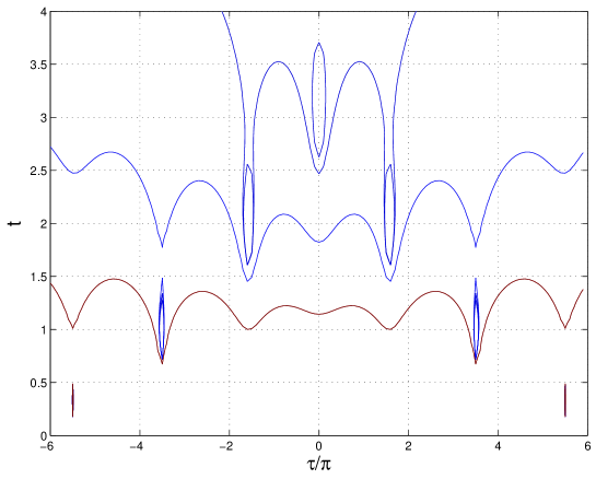
Figure 1: Contour plot of the potential, given by Eq. (3.34), in the ($t$,$\tau$) plane for $m=-1$, $k=20$.

These statements can be easily checked in Figure 1, where we show a contour plot of the scalar potential, as given by Eq. (3.34), in the $t$, $\tau$ plane. We have chosen $m=-1$, $k=20$, and we can see that, following Eq. (3.42), the number of minima is very close to $|\kappa|/\pi$, with $\kappa=k/m=-20$; moreover, and according to Eq. (3.41), the value of $t_{\rm max}$ is given by ${\rm ln}|\kappa|$ and, also, we can see in the figure that Eq. (3.43) is fulfilled. Finally we have checked that all these minima preserve supersymmetry with negative vacuum energy.

More precisely, from Eq. (2.24) the potential value at any one of these minima is given by

$$V_{\rm min}=-\frac{21C^{2}}{t^{5}}\frac{(t+1)^{2}+\tau^{2}}{(2t+7)^{2}}\;,$$ (3.44)

and is, hence, always strictly negative. Also, since from Eq. (3.38) $\tau$ increases as $t$ decreases, the absolute minimum will be the one with the smallest value of $t$. For $\kappa>0$, or sufficiently negative $\kappa\mathrel{\hbox to0.0pt{\raise 2.15277pt\hbox{$<$}\hss}{\lower 2.15277pt\hbox{$\sim$}}}-5$, this is always a complex minimum, $\tau\neq 0$. Also note that the two minima for a given solution of $t$ are degenerate, since they only differ by a sign of the imaginary part $\tau$.

To summarize, for our simple model, the structure of minima is controlled by the parameter $\kappa$, defined in Eq. (2.9). To have minima compatible with the supergravity approximation, that is, minima satisfying Eq. (2.15), we need $|\kappa|\mathrel{\hbox to0.0pt{\raise 2.15277pt\hbox{$>$}\hss}{\lower 2.15277pt\hbox{$\sim$}}}1$. The number of minima is roughly given by $|\kappa|/\pi$ and the real part $t$ is always in the range $t\in[0,t_{\rm max}]$, where, roughly, $t_{\rm max}\sim\ln|\kappa|$. For $\kappa<0$ a special real minimum with $t=t_{\rm max}$ and $\tau=0$ exists; all other minima are complex. All minima preserve supersymmetry and have a negative cosmological constant. The absolute minimum is the one with the lowest value of $t$, and generally has a non-vanishing imaginary part, $\tau\neq 0$.

3.2 Non-universal bulk moduli

We now move on to a more realistic model with seven individual moduli

$$T^{a}=t_{a}+i\tau_{a}\;,$$ (3.45)

where $a,b,\dots=1,\dots,7$. The real parts $t_{a}$ can be interpreted as the seven radii of the torus that underlies the construction of the $G_{2}$ manifold. The Kähler potential and superpotential are now given by

$$K = -\sum_{a=1}^{7}\ln(T^{a}+\bar{T}^{a})$$ (3.46)

$$W = \sum_{a=1}^{7}w_{(a)}\;,$$ (3.47)

where the function $w$ is defined in Eq. (2.14) and we have written

$$w_{(a)}=w(m_{a},k_{a},T^{a})\;,$$ (3.48)

for ease of notation. The F-terms take the form

$$F_{a}=w_{(a)}^{\prime}-\frac{1}{2t_{a}}W\;,$$ (3.49)

while the scalar potential can be written as

$$V=\frac{1}{32\Pi_{b=1}^{7}t_{b}}\left\{\sum_{a}\left[t_{a}^{2}|w_{(a)}^{\prime}|^{2}-t_{a}\Re(w_{(a)}^{\prime}\bar{W})\right]+|W|^{2}\right\}\;.$$ (3.50)

Here $w^{\prime}$ denotes the derivative of $w$ with respect to its last argument. Analyzing the general vacuum structure of this model would be rather cumbersome given the large parameter space. We will not attempt to do this but instead present a number of examples.

Consider a “universal” choice of parameters, independent of the index $a$, that is,

$$m_{a}=m\;,\qquad k_{a}=k$$ (3.51)

for some real $m$, $k$ and all $a=1,\dots,7$. Then the F-terms (3.49) can be written as

$$F_{a}=w^{\prime}(m,k,T^{a})-\frac{1}{2t_{a}}\sum_{b=1}^{7}w(m,k,T^{b})\;.$$ (3.52)

Now take any of the supersymmetric minima $T=t+i\tau$ found in the previous subsection for the universal case. Comparison of Eqs. (3.29) and (3.52) then shows that setting

$$T^{a}=T\;,$$ (3.53)

for all $a=1,\dots,7$ solves all seven equations $F_{a}=0$. Hence, every supersymmetric minimum of the universal single $T$ model leads to a supersymmetric extremum for the case with seven moduli $T_{a}$, provided the parameters have been chosen universally, as in Eq. (3.51). It can be shown from Eqs. (2.22) and (2.23) that these extrema are indeed minima if $t$ is sufficiently large, that is, roughly $t\mathrel{\hbox to0.0pt{\raise 2.15277pt\hbox{$>$}\hss}{\lower 2.15277pt\hbox{$\sim$}}}1$. As in the universal case, the cosmological constant is always negative. As discussed at the end of Section 2, these minima still exist for a non-universal choice of parameters sufficiently close to the universal one.

Allowing seven $T$-moduli also opens up qualitatively new possibilities compared to the universal case. Consider the conditions (2.25) for supersymmetric minima with vanishing cosmological constant. Applied to the present case they lead to moduli values

$$T^{a}=\ln\left|\frac{k_{a}}{m_{a}}\right|+\pi in_{a}$$ (3.54)

where $n_{a}$ is an integer which is even for positive $k_{a}/m_{a}$ and odd otherwise. In addition, vanishing of the real and imaginary part of the superpotential implies that

$$\sum_{a=1}^{7}m_{a}\left(1+\ln\left|\frac{k_{a}}{m_{a}}\right|\right) = 0$$ (3.55)

$$\sum_{a=1}^{7}m_{a}n_{a} = 0\;.$$ (3.56)

The first of these conditions is the usual fine-tuning required to make the cosmological constant vanish. It constrains parameters to a particular hyper-surface in parameter space. With favourable choices for the signs of $k_{a}/m_{a}$, the second condition will have an infinite number of solutions. They correspond to an infinite number of degenerate supersymmetric minima with vanishing cosmological constant that differ by integer shifts in the axion directions.

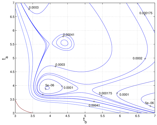
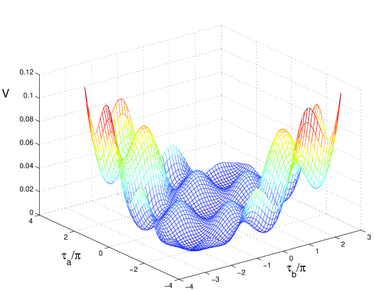
Figure 2: Contour plot of the potential, given by Eq. (3.50), as a function of $t_{a}$ ($a=1,2,3$) and $t_{b}$ ($b=4,5,6,7$) for $m_{a}=4$, $k_{a}=200$, $m_{b}=-3$, $k_{b}=-150$. The imaginary parts of all fields have been set to zero, where we have a minimum.

Figure 3: Plot of the potential, given by Eq. (3.50), as a function of $\tau_{a}$, $\tau_{b}$ for the same values of parameters as in the previous figure. The real parts of the fields have been set to their minimum values at ${\rm ln}|k_{i}/m_{i}|$, $i=a,b$.

We present an example of this behaviour in Figures 3,3, where we have split the moduli into two types, $a=1,2,3$ and $b=4,5,6,7$, in order to make the graphics manageable. In Figure 3 we show a contour plot of the potential, as given by Eq. (3.50), in the $t_{a}$, $t_{b}$ plane, for values of the parameters $m_{a}=4$, $k_{a}=200$, $m_{b}=-3$, $k_{b}=-150$, with the imaginary parts of the fields, $\tau_{a}$, $\tau_{b}$ fixed at zero. In this way, both Eqs (3.55,3.56) are fulfilled. Moreover, a minimum is found at the predicted values for the moduli, given by Eq. (3.54) with $n_{a}=n_{b}=0$, which, in this case, becomes $t_{a}=t_{b}=3.9$. We can also see that for larger values of $t_{a}$ a maximum appears, while for larger $t_{b}$ we have a saddle point. In Figure 3, where we show the potential as a function of $\tau_{a}$, $\tau_{b}$ for $t_{a}$, $t_{b}$ fixed at their minimum values, we can check how $\tau_{a}=\tau_{b}=0$ does indeed correspond to a minimum which, however, is degenerate with those at $\tau_{a}=\tau_{b}=2n\pi$ for $n$ integer. There exists, therefore, in these cases, an array of degenerate minima with zero cosmological constant. An obvious consequence of this pattern should be the formation of domain walls between the different minima.

Comparison of Eqs (2.6) and (3.56) show that all these minima correspond to vanishing external flux. From our general discussion, we also know that supersymmetric minima, although with negative cosmological constant, exist in a neighbourhood of the hypersurface (3.55) in parameter space.

4 Including blow-up moduli

We should now add blow-up moduli to the models of the previous section. We begin with the universal case.

4.1 The universal case

An obvious extension of the simple model with a single bulk modulus $T$ presented in Section 3.1 adds a second field $U$ as the typical representative of a blow-up modulus. Split into real and imaginary parts we write

$$T = t+i\tau$$ (4.57)

$$U = u+i\nu\;.$$ (4.58)

The model is then defined by

$$K = -7\ln(T+\bar{T})+b\frac{(U+\bar{U})^{2}}{(T+\bar{T})^{2}}$$ (4.59)

$$W = w(m,k,T)+w(\mu,l,U)\;,$$ (4.60)

where $b$ is a real positive constant. To make contact with the full model later on we will need to set $b=8I$, where $I$ is the number of blow-up moduli. However, for the purpose of this sub-section, we will treat $b$ as a phenomenological parameter. It is useful to introduce the ratio

$$\epsilon=\frac{u}{t}\;,$$ (4.61)

of blow-up and bulk modulus. Recall that the above Kähler potential should be viewed as an expansion in $\epsilon$ where terms of order $\epsilon^{4}$ and higher have been neglected. In accordance with the general constraint (2.16) we should, therefore, work in the region of moduli space where

$$b\epsilon^{2}\ll 1\;.$$ (4.62)

Note that corrections of ${\cal O}(\epsilon^{4})$ to $K$ will lead to ${\cal O}(\epsilon^{2})$ terms in the scalar potential. Hence, on the basis of the Kähler potential (4.59), we can reliably compute the scalar potential only up to terms of ${\cal O}(\epsilon)$. Subsequent formulae will be quoted to this order.

It is crucial to check that relevant features of the scalar potential, such as minima arising at ${\cal O}(\epsilon)$, are stable under inclusion of terms of ${\cal O}(\epsilon^{2})$ and higher, so that (4.62) is indeed satisfied to the necessary degree. In practice, we will add a hypothetical correction

$$\delta K=d\frac{(U+\bar{U})^{4}}{(T+\bar{T})^{4}}$$ (4.63)

to the Kähler potential (4.59), where $d$ is a real number, and compute the scalar potential up to order $\epsilon^{2}$ by including this correction. We will then compare the potentials at ${\cal O}(\epsilon)$ and ${\cal O}(\epsilon^{2})$, and only accept minima if they consistently arise at both orders and for a reasonable range of $d$.

For the Kähler potential (4.59), and a general superpotential, the F-terms, to order $\epsilon$, are given by

$$F_{T} = W_{T}-\frac{7}{2t}W$$ (4.64)

$$F_{U} = W_{U}+\frac{b\epsilon}{t}W\;.$$ (4.65)

To this order, the scalar potential reads

$$V=\frac{1}{112t^{5}}\left\{\frac{1}{2}|W_{T}|^{2}+\frac{7}{4b}|W_{U}|^{2}+2\epsilon\Re(W_{T}\bar{W}_{U})-\frac{7}{2t}\Re(W_{T}\bar{W})-\frac{7\epsilon}{2t}\Re(W_{U}\bar{W})+\frac{7}{2t^{2}}|W|^{2}\right\}\;.\$$ (4.66)

The explicit expressions for the F-terms and the scalar potential are fairly complicated and are given in Appendix A. Inspection of the general scalar potential (2.17) shows that

$$\frac{\partial V}{\partial\tau}(\tau=0,\nu=0)=0\;,\qquad\frac{\partial V}{\partial\nu}(\tau=0,\nu=0)=0\;,$$ (4.67)

so the potential is extremized in the imaginary directions at $\tau=\nu=0$. Here we will focus on this real case, that is, we will set $\tau=\nu=0$. Equations (A.5)–(A.8) show that then the imaginary parts of the F-terms are automatically zero, that is, $\Im(F_{T})=\Im(F_{U})=0$, while the real parts simplify to

$$\Re(F_{T}) = -\frac{m}{2}\left[5+\kappa\left(2+\frac{7}{t}\right)e^{-t}+\frac{7}{t}(Mu+Le^{-u})\right]$$ (4.68)

$$\Re(F_{U}) \simeq m\left[M-Le^{-u}+\frac{b\epsilon}{t}(t+\kappa e^{-t})\right]\;.$$ (4.69)

Here we have normalized our parameters with respect to the flux $m$ by defining

$$\kappa=\frac{k}{m}\;,\qquad L=\frac{l}{m}\;,\qquad M=\frac{\mu}{m}\;.$$ (4.70)

For vanishing imaginary parts the potential (A) then simplifies to

$$V = \frac{C^{2}}{t^{5}}\left\{1+\kappa\left[5+\frac{7}{t}\right]e^{-t}\pm L\left[\frac{3u}{t}+\frac{7}{t}\right]e^{-u}+K^{2}\left[1+\frac{7}{t}+\frac{7}{t^{2}}\right]e^{-2t}\right.$$

$$\qquad+7L^{2}\left[\frac{1}{2b}+\frac{u}{t^{2}}+\frac{1}{t^{2}}\right]e^{-2u}\pm LK\left[\frac{4u}{t}+\frac{7}{t}+\frac{7u}{t^{2}}+\frac{14}{t^{2}}\right]e^{-t-u}$$

$$\qquad\left.+\frac{7M^{2}}{2b}+4M\frac{u}{t}+KM\left[\frac{3u}{t}+\frac{7u}{t^{2}}\right]e^{-t}+LM\left[\frac{7u^{2}}{t^{2}}+\frac{7u}{t^{2}}-\frac{7}{b}\right]\right\}\;.$$

After minimizing this potential in $t$ and $u$ we still, of course, have to check whether the extrema in the imaginary directions are indeed minima.

Let us start by looking for supersymmetric minima with vanishing cosmological constant, that is, solutions to the equations $W_{T}=0$, $W_{U}=0$ and $W=0$. The first two of these equations immediately imply that

$$T = \ln\left|\kappa\right|+\pi ip$$ (4.72)

$$U = \ln\left|\frac{L}{M}\right|+\pi iq\;,$$ (4.73)

where $p$ ($q$) is an integer which is even for $\kappa>0$ ($L>0$) and odd otherwise. Vanishing of the superpotential leads to the two conditions

$$m\left(1+\ln\left|\kappa\right|\right)+\mu\left(1+\ln\left|\frac{l}{\mu}\right|\right) = 0\;,$$ (4.74)

$$mp+\mu q = 0\;.$$ (4.75)

For fixed (integer) flux $m$ and $\mu$ the first of these equations can always be solved for appropriate choices of the parameters $k$ and $l$. The second equation has an infinite number of other solutions when the signs of $\kappa$ and $\mu/l$ are chosen appropriately. In particular, for $\kappa>0$ and $\mu/l>0$, we can take $p=q=0$ and obtain a real supersymmetric minimum with vanishing cosmological constant. Hence, by tuning in parameter space, we can have supersymmetric minima with vanishing cosmological constant, infinitely degenerate by integer shifts in the axion directions. From Eqs. (2.6) and (4.75) all those minima correspond to vanishing external flux. In the neighbourhood in parameter space of each such minimum there will be supersymmetric minima with negative cosmological constant. We note that their existence is independent of the Kähler potential. Hence, we do not need to require that $b\epsilon^{2}\ll 1$, although this could be easily arranged by choosing parameters. However, unless $b\epsilon^{2}\ll 1$, we are unable to explicitly write down the scalar potential close to these minima.

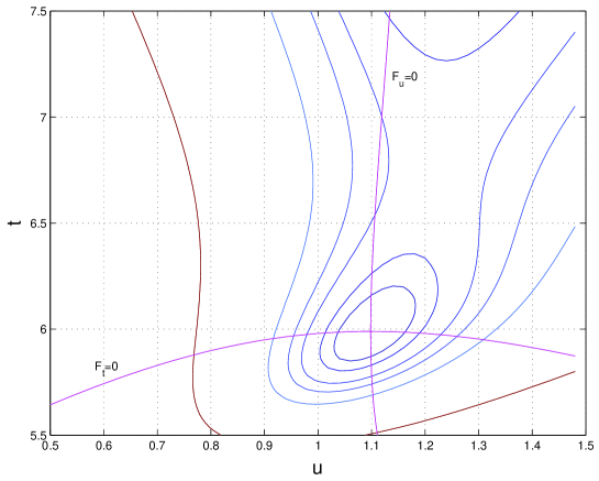
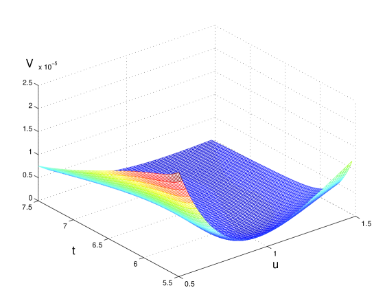
Figure 4: Contour plot of the potential, given by Eq. (4.1), in the $t$, $u$ plane, for $m=3$, $k=1200$, $\mu=-10$, $l=-30$. We have also plotted the conditions $F_{T}=F_{U}=0$ in order to show the supersymmetric character of the minimum. The imaginary parts of all fields have been set to zero.

Figure 5: Plot of the potential, given by Eq. (4.1), as a function of $t$, $u$ for the same values of parameters as in the previous figure. The minimum corresponds to Eqs (4.72,4.73,4.74) being fulfilled.

We confirm the previous statements by showing an explicit example of a real supersymmetric minimum with vanishing cosmological constant in Figures 5,5. The choice of parameters is such that Eq. (4.74) is satisfied, and the values of the fields correspond to $t=\ln(\kappa)=5.99$, $u=\ln(l/\mu)=1.1$, in agreement with Eqs (4.72,4.73). In Figure 5, the conditions $F_{T}=F_{U}=0$ are also plotted to show that the minimum is indeed supersymmetric. Here we are considering $b=8$, i.e. $I=1$, and we have checked that corrections of order $\epsilon^{2}$ and higher do not affect the existence and position of the minimum.

Let us now drop the condition of vanishing cosmological constant and focus on real supersymmetric minima, that is, $\tau=\nu=0$. The relevant F-terms have been given in Eqs. (4.68) and (4.69). It can be shown that solutions to the F-equations are always minima for the model at hand. A very rough approximation to the equation $\Re(F_{U})=0$ leads to the solution

$$u\simeq\ln\left|\frac{L}{M}\right|\;,$$ (4.76)

which coincides with the result (4.73) one obtains for vanishing cosmological constant. Since we have set the phases to zero, it exists only if $L$ and $M$ have the same sign. Inserting this into the equation $\Re(F_{T})=0$ we find $t$ is determined by

$$5+\kappa\left(2+\frac{7}{t}\right)e^{-t}+\frac{7M}{t}\left(1+\ln\left|\frac{L}{M}\right|\right)=0\;.$$ (4.77)

For sufficiently small $M$ this can be solved for negative $\kappa$ leading roughly to $t\sim t_{\rm max}$, where $t_{\rm max}$ was defined in Eq. (3.40). Hence, we expect supersymmetric minima for $\kappa<0$ and $L$, $M$ having the same sign. Further, since $t_{\rm max}\sim\ln|\kappa|$, we typically need to have $|\kappa|\gg 1$ in order to satisfy the constraint $b\epsilon\ll 1$.

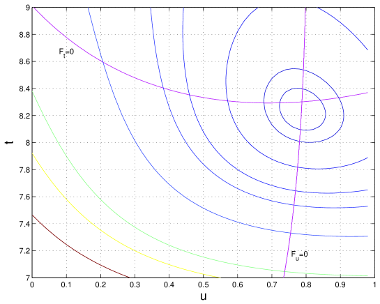
Figure 6: Contour plot of the potential, given by Eq. (4.1), in the ($t$, $u$) plane, for $m=-1$, $k=1000$, $\mu=3$, $l=6$. We also plot the conditions $F_{T}=F_{U}=0$ to show the supersymmetric character of the minimum. The imaginary parts of all fields have been set to zero.

This kind of supersymmetric minima, with negative cosmological constant, is shown in Figure 6 for values of the parameters given by $m=-1$, $k=1000$, $\mu=3$, $l=6$ (i.e. $L,M<0$). The minimum in the $u$ direction is quite close to the value given by Eq. (4.76), whereas Eq. (4.77) constitutes a rough approximation for the corresponding value of $t$ (given by $t=8.25$). Similar minima can be obtained, as already explained, for $\kappa<0$ and the opposite choice of signs for $L,M$. And, again, we have chosen $I=1$ in order to keep our perturbative expansion well under control.

For $\kappa>0$, using the relations (4.72) with $p=0$ and (4.74), which describe the supersymmetric minima with vanishing cosmological constant, Eq. (4.77) is identically satisfied, as it should be. Perturbing away from this special point in parameter space one can still find solutions to Eq.(3.36) that are characterized by $\kappa>0$ and $M<0$. They are precisely the supersymmetric minima close to the ones with vanishing cosmological constant whose existence we have inferred above from general argument.

In summary, we expect three classes of supersymmetric minima, depending on the signs of the various parameters but all with $L/M>0$. For $\kappa<0$ we can have either sign of $M$ while for $\kappa>0$ supersymmetric solutions only exist for $M<0$.

We now turn to the search of minima with broken supersymmetry. Unfortunately, here we can not count on the F-equations being fulfilled in order to look for minima, however, as it turns out, a good starting point is to look for solutions to the condition $F_{T}=0$ in order to find minima of the potential (4.1). As it has already been pointed out, in order to keep the supergravity approximation, Eq. (2.15), valid, as well as to suppress higher order terms in the Kähler potential, Eq. (2.16), we need $t$ to be large at the minimum (at least of order 10). This translates into a large value for $\kappa$. At the same time we need to keep the value of $u$ of order 1, and the number of blow-up moduli below about 10, in order to comply with the condition $b\epsilon^{2}\ll 1$. This also guarantees the smallness of the mixing terms between $t$ and $u$ in the scalar potential, and explains why the minimization along the $t$ direction is almost unchanged with respect to the purely supersymmetric case.

Therefore minima with broken supersymmetry appear for large $\kappa$ (and $F_{T}\sim 0$) and $l$,$\mu$ of the same order of magnitude. As for their signs, we have found only minima for $l<0$, $\mu>0$ whereas the opposite choice gives rise to a runaway potential for increasing values of $u$.

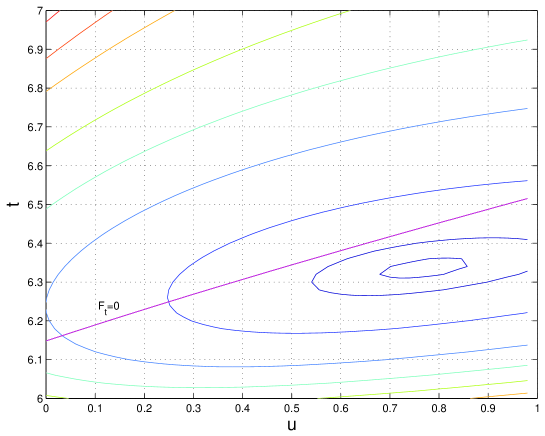
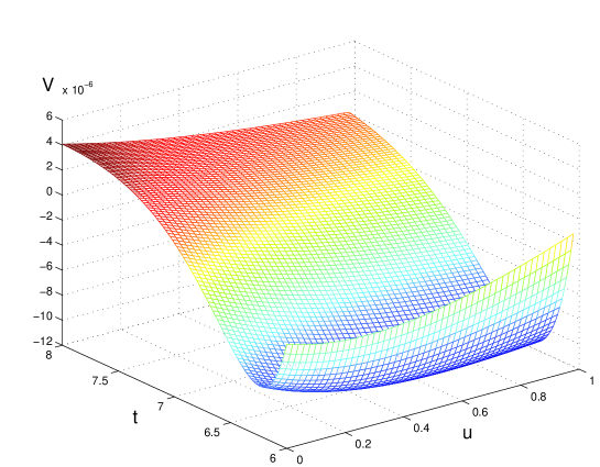
Figure 7: Contour plot of the potential, given by Eq. (4.1), in the ($t$, $u$) plane, for $m=-1$, $k=1000$, $\mu=1$, $l=-1.5$. We have also added the condition $F_{T}=0$. The imaginary parts of all fields have been set to zero, where we have a minimum.

Figure 8: Plot of the potential, given by Eq. (4.1), as a function of $t$, $u$ for the same values of parameters as in the previous figure.

A typical example of what has just been described is shown in Figures 8,8, where we plot both the contour and the shape of the potential given by Eq. (4.1) for $m=-1$, $k=1000$, $\mu=1$, $l=-1.5$ as a function of $t$ and $u$ (their imaginary parts having been set to zero). In Figure 8 we have also plotted the constraint $F_{T}=0$ in order to show how close it is to the minimum (whereas $F_{U}=0$ lies well outside the plot). All the minima with broken supersymmetry that we have found have a negative cosmological constant.

Finally we would like to add a further comment on the stability of our results. As already mentioned several times, we are imposing the constraint $b\epsilon^{2}\ll 1$ in order to guarantee that (as yet unknown) higher order corrections to the Kähler potential will not spoil the results presented here. This, in turn, means that we have a tight restriction on the number of blow-up moduli (given by $I$, with $b=8I$) allowed in our models. We have found that, in order to achieve $u_{\rm min}\sim 1$, $I=1$ becomes almost the only choice. We can still find minima with $0<u_{\rm min}<1$ for $I\leq 10$, however larger values of $I$ would result in the minima shifting to negative values of $u$. There are, though, plenty of examples in the literature of compact $G_{2}$ manifolds with a small number of blow-ups, and while the precise Kähler potential for those cases is not known, we expect it to resemble the one used here. In that respect our results should be taken from a purely phenomenological point of view. Once a complete formula for the Kähler potential is known, it should be very easy to incorporate it to our analysis, and it would be surprising if the results differed substantially from those presented here.

4.2 The general model

We are now ready to analyze the general model defined by the Kähler potential (2.9) and the superpotential (2.13), which we write as

$$W=\sum_{a=1}^{7}w_{(a)}+\sum_{i=1}^{I}w_{(i)}\;,$$ (4.78)

where $w_{(a)}=w(m_{a},k_{a},T^{a})$ and $w_{(i)}=w(\mu_{i},l_{i},U^{i})$, and the function $w$ has been defined in Eq. (2.14). The F-terms to order $\epsilon$ then take the form

$$F_{a} = w_{(a)}^{\prime}-\frac{1}{2t_{a}}W$$ (4.79)

$$F_{i} = w_{(i)}^{\prime}+4f^{i}u_{i}W$$ (4.80)

with $f^{i}$ given in Eq. (2.10). For the scalar potential we find

$$V = \frac{1}{32\Pi_{c=1}^{7}t_{c}}\left\{\sum_{a=1}^{7}\left[t_{a}^{2}|w_{(a)}^{\prime}|^{2}-t_{a}\Re(w_{(a)}^{\prime}\bar{W})\right]+\sum_{i=1}^{I}\left[\frac{|w_{(i)}^{\prime}|^{2}}{8f^{i}}-u_{i}\Re(w_{(i)}^{\prime}\bar{W})\right]\right.$$ (4.81)

$$\left.\qquad\qquad+2\sum_{a=1}^{7}\sum_{i=1}^{I}p_{ia}t_{a}u_{i}\Re(w_{(a)}^{\prime}\bar{w}_{(i)}^{\prime})+|W|^{2}\right\}\;.$$

We will not attempt a general classification of all minima of this potential but rather present various classes of examples. We start with the supersymmetric minima with vanishing cosmological constant, characterized by the equations $w_{(a)}^{\prime}=0$, $w_{(i)}^{\prime}=0$ and $W=0$. The field values are easily solved for and are given by

$$T^{a} = \ln\left|\frac{k_{a}}{m_{a}}\right|+\pi in_{a}$$ (4.82)

$$U^{i} = \ln\left|\frac{l_{i}}{\mu_{i}}\right|+\pi in_{i}\;,$$ (4.83)

where $n_{a}$ are even (odd) integers for $k_{a}/m_{a}$ positive (negative) and, similarly, $n_{i}$ are even (odd) integers for $l_{i}/\mu_{i}$ positive (negative). Vanishing of the real and imaginary parts of the superpotential implies

$$\sum_{a=1}^{7}m_{a}\left(1+\ln\left|\frac{k_{a}}{m_{a}}\right|\right)+\sum_{i=1}^{I}\mu_{i}\left(1+\ln\left|\frac{l_{i}}{\mu_{i}}\right|\right) = 0$$ (4.84)

$$\sum_{a=1}^{7}m_{a}n_{a}+\sum_{i=1}^{I}\mu_{i}n_{i} = 0\;.$$ (4.85)

As in the analogous cases before, the first of these conditions is the usual fine-tuning in parameter space required to set the cosmological constant to zero, while the second has infinitely many solutions for favourable signs of $k_{a}/m_{a}$ and $l_{i}/\mu_{i}$ (or appropriate choices of the flux). We have hence found an infinite number of supersymmetric minima with vanishing cosmological constant that differ by integer shifts in the axion directions. As before, all those minima correspond to vanishing external flux, as Eq. (2.6) shows. In a neighbourhood of the surface in parameter space defined by Eq. (4.84) there exist supersymmetric minima with negative cosmological constant. We stress that the existence of these supersymmetric minima does not depend on the form of the Kähler potential and is, hence, not subject to the constraint (2.16) in moduli space. Consequently, these minima exist for an arbitrary number $I$ of blow-up moduli and, in particular, for the specific model detailed in Table 1.

In our discussion of the universal model with a single $T$ and $U$ modulus, we have encountered three classes of supersymmetric minima characterized by the sign of the parameters. Above, we have shown that the analog of one of these classes, namely the one that includes supersymmetric minima with vanishing cosmological constant, also exists in the general case. What about the other two cases? We can construct examples for those cases by generalizing the results for the universal case. We choose specific parameters, such that

$$k_{a}=k\;,\qquad m_{a}=m\;,\qquad l_{i}=\frac{7}{I}l\;,\qquad\mu_{i}=\frac{7}{I}\mu\;,$$ (4.86)

for all $a$ and $i$ and universal parameters $k$, $m$, $l$ and $\mu$. For these parameters, we compute the F-terms at the universal point

$$T^{a}=T\;,\qquad U^{i}=U\;,$$ (4.87)

in field space. We find that $W=7\tilde{W}$ where

$$\tilde{W}=w(k,m,T)+w(l,\mu,U)\;,$$ (4.88)

and

$$F_{a} = w^{\prime}(k,m,T)-\frac{7}{2t}\tilde{W}$$ (4.89)

$$F_{i} = \frac{7}{I}\left[w^{\prime}(l,\mu,U)+\frac{bu}{t^{2}}\tilde{W}\right]\;,$$ (4.90)

where $b=8I$. Comparison with the universal F-terms (4.64) and (4.65) then shows that every solution $(T,U)$ to the universal F-equations for parameters $k$, $m$, $l$, $\mu$ gives rise to a solution of the general F-equations via the identification (4.86), (4.87). We still have to show whether these solutions, if minima in the universal case, remain minima for the general model. To do this, we evaluate the expressions (2.22) and (2.23) for the second derivative of the potential at supersymmetric minima, using the general model defined by Eqs. (2.9) and (2.13) but specializing to universal parameters (4.86) and fields (4.87). The result is compared with that of an analogous calculation for the universal $(T,U)$ model. This comparison shows that minima of the universal $(T,U)$ model indeed remain minima of the general model at the universal point if $t$ is sufficiently large and $\epsilon$ small. As before, these minima still exist for non-universal parameters sufficiently close to the universal choice (4.86). We note that the phenomenological parameter $b$ in the universal Kähler potential (4.59) is identified as $b=8I$ under this correspondence, where we recall that $I$ is the number of blow-up moduli. In our analysis of the universal case we found that consistent minima, stable under higher-order corrections to the Kähler potential, exist for $b\mathrel{\hbox to0.0pt{\raise 2.15277pt\hbox{$<$}\hss}{\lower 2.15277pt\hbox{$\sim$}}}40$ ($b\mathrel{\hbox to0.0pt{\raise 2.15277pt\hbox{$<$}\hss}{\lower 2.15277pt\hbox{$\sim$}}}80$ if one tolerates a small value of $u$). This translates into an upper bound of $I\mathrel{\hbox to0.0pt{\raise 2.15277pt\hbox{$<$}\hss}{\lower 2.15277pt\hbox{$\sim$}}}5$ ($I\mathrel{\hbox to0.0pt{\raise 2.15277pt\hbox{$<$}\hss}{\lower 2.15277pt\hbox{$\sim$}}}10$ allowing small values of $u$) for the maximal number of blow-up moduli for which we can construct supersymmetric minima in this way. In summary, we conclude that the supersymmetric minima with negative cosmological constant can indeed be extended to complete models with up to $5$ (or $10$) blow-up moduli.

Can the supersymmetry breaking minima with negative cosmological constant we found in the universal case be generalized to the full model? Let us consider a minimum for the universal model with parameters $m$, $k$, $\mu$, $l$ and field values $T$ and $U$ and analyze the general model at universal parameter values (4.86) and universal field values (4.87). It is straightforward to show that

$$\frac{\partial V}{\partial U^{i}}=0\;,$$ (4.91)

using the fact that the $U$ derivative of the universal potential (4.66) vanishes and identifying $b=8I$, as before. Unfortunately, the $T^{a}$ derivatives of $V$ do not vanish exactly at the universal point, due to the non-trivial coupling between the $T$ and $U$ moduli encoded in the coefficients $p_{ia}$. However, it can be shown that $\partial V/\partial T^{a}$ consists of terms either of order $\epsilon$ or suppressed by inverse powers of $t$. Hence, for sufficiently large $t$ and small $\epsilon$ the derivatives $\partial V/\partial T^{a}$ are small and there will be an extremum for field values close the universal choice. Moreover, under the same conditions on $t$ and $\epsilon$ these will still be minima. We conclude, that non-supersymmetric minima with negative cosmological constant can be generalized to the full model. As above, the constraint on the parameter $b$, necessary for consistent minima of the universal model to exist, translates into a bound of $I\mathrel{\hbox to0.0pt{\raise 2.15277pt\hbox{$<$}\hss}{\lower 2.15277pt\hbox{$\sim$}}}5$ ($I\mathrel{\hbox to0.0pt{\raise 2.15277pt\hbox{$<$}\hss}{\lower 2.15277pt\hbox{$\sim$}}}10$ allowing small $u$ values) on the number $I$ of blow-up moduli for which we can obtain such non-supersymmetric minima.

5 Conclusion

In this paper we have analyzed the vacuum structure of four-dimensional $N=1$ supergravity theories originating from M-theory on $G_{2}$ spaces, with a superpotential from flux and membrane instanton effects. We have focused on $G_{2}$ spaces which are constructed by blowing up $G_{2}$ orbifolds. These spaces have two different types of moduli, namely “bulk” moduli $T^{a}$ associated with the underlying orbifold and “blow-up” moduli $U^{i}$ which measure the size and orientation of the blow-ups.

We have been starting the analysis with a simple toy model consisting of a single bulk modulus $T$, generalizing to seven bulk moduli $T^{a}$, then including blow-up moduli, first in a universal model with a single bulk and blow-up modulus $(T,U)$, and, finally, studying the full model. Our main result is that minima with negative cosmological constant can be found. They exist for both supersymmetry preserved as well as broken and, after appropriate tuning of parameters, supersymmetric minima with vanishing cosmological constant exist for the general model, as well as for most of the simpler toy models. In constructing consistent minima we had to respect one technical constraints on the moduli space. The typical ratio $\epsilon=u/t$ of the a bulk modulus $t$ and a blow-up modulus $u$ had to be smaller than one since the Kähler potential has only been calculated to leading order in $\epsilon$. The supersymmetric minima with vanishing cosmological constant are unaffected by this constraint since they only depend on the superpotential. However, for all other minima it implies an upper bound on the number $I$ of blow-up moduli. Moreover, we need a large parameters $k_{a}$ multiplying the $T_{a}$ instanton contributions in the superpotential in order to generate sufficiently large values for the bulk moduli. We expect both restrictions could be avoided if the exact Kähler potential was known.

Although we did obtain supersymmetry breaking minima we have not been able to find any examples with a positive cosmological constant. From our experience a positive cosmological constant cannot be achieved in the given setting, using a combination of flux and membrane instantons. In analogy with the IIB construction of Ref. [21], this can presumably be achieved by adding wrapped (anti) M5-branes to our set-up. Work in this direction is in progress.

Acknowledgments A. L. and B. d. C.  are supported by PPARC Advanced Fellowships. S. M. is supported by a Royal Society postdoctoral fellowship.

Appendix

Appendix A Full potential for a single bulk and blow-up modulus

We consider the case with a single bulk modulus $T$ and a single blow-up modulus $U$, split into real and imaginary parts as

$$T = t+i\tau$$ (A.1)

$$U = u+i\nu\;.$$ (A.2)

The model is defined by the Kähler potential and superpotential

$$K = -7\ln(T+\bar{T})+b\frac{(U+\bar{U})^{2}}{(T+\bar{T})^{2}}$$ (A.3)

$$W = mT+ke^{-T}+\mu U+le^{-U}\;,$$ (A.4)

where $m$, $k$, $\mu$, $l$ and b are real constants. We then find for the F-terms

$$\Re(F_{T}) = -\frac{m}{2}\left[5+\kappa\left(2+\frac{7}{t}\right)\cos(\tau)e^{-t}+\frac{7}{t}(Mu+L\cos(\nu)e^{-u})\right]$$ (A.5)

$$\Im(F_{T}) = \frac{m}{2}\left[K\left(2+\frac{7}{t}\right)\sin(\tau)e^{-t}-\frac{7}{t}(\tau+M\nu-L\sin(\nu)e^{-u})\right]$$ (A.6)

$$\Re(F_{U}) \simeq m\left[M-L\cos(\nu)e^{-u}+\frac{bu}{t}(t+\kappa e^{-t}\cos(\tau))\right]$$ (A.7)

$$\Im(F_{U}) \simeq \left[L\sin(\nu)e^{-u}+\frac{bu}{t^{2}}(\tau-\kappa\sin(\tau)e^{-t}+M\nu)\right]\;,$$ (A.8)

where

$$\kappa=\frac{k}{m}\;,\qquad L=\frac{l}{m}\;,\qquad M=\frac{\mu}{m}\;.$$ (A.9)

The scalar potential is given by

$$V = \frac{C^{2}}{t^{5}}\left\{1+\frac{7\tau^{2}}{t^{2}}+\kappa\left[5\cos(\tau)+(\cos(\tau)-\tau\sin(\tau))\frac{7}{t}-\frac{14\tau\sin(\tau)}{t^{2}}\right]e^{-t}\right.$$

$$\qquad+L\left[\left(3\cos(\nu)-\frac{7\sin(\nu)\tau}{t}\right)\frac{v}{t}+\frac{7\cos(\nu)}{t}-\frac{14\tau\sin(\nu)}{t^{2}}\right]e^{-u}$$

$$\qquad+K^{2}\left[1+\frac{7}{t}+\frac{7}{t^{2}}\right]e^{-2t}+7L^{2}\left[\frac{1}{2b}+\frac{u}{t^{2}}+\frac{1}{t^{2}}\right]e^{-2u}$$

$$\qquad+KL\cos(\tau-\nu)\left[\left(4+\frac{7}{t}\right)\frac{u}{t}+\frac{7}{t}+\frac{14}{t^{2}}\right]e^{-t-u}+M^{2}\left[\frac{7}{2b}+\frac{7\nu^{2}}{t^{2}}\right]$$

$$\qquad+M\left[\frac{4u}{t}+\frac{14\tau\nu}{t^{2}}\right]+KM\left[\frac{3\cos(\tau)u}{t}-\frac{14\sin(\tau)\nu}{t^{2}}-\frac{7\sin(\tau)\nu}{t}+\frac{7\cos(\tau)u}{t^{2}}\right]e^{-t}$$

$$\left.\qquad+LM\left[\frac{7\cos(\nu)u^{2}}{t^{2}}+\frac{7\cos(\nu)u}{t^{2}}-\frac{7\cos(\nu)}{b}-\frac{7\sin(\nu)\nu u}{t^{2}}-\frac{14\sin(\nu)\nu}{t^{2}}\right]e^{-u}\right\}\;.$$

References

- [1] S. Ferrara, L. Girardello and H. P. Nilles, “Breakdown Of Local Supersymmetry Through Gauge Fermion Condensates,” Phys. Lett. B 125 (1983) 457.
- [2] J. P. Derendinger, L. E. Ibanez and H. P. Nilles, “On The Low-Energy D = 4, N=1 Supergravity Theory Extracted From The D = 10, N=1 Superstring,” Phys. Lett. B 155, 65 (1985).
- [3] M. Dine, R. Rohm, N. Seiberg and E. Witten, “Gluino Condensation In Superstring Models,” Phys. Lett. B 156 (1985) 55.
- [4] C. Kounnas and M. Porrati, “Duality And Gaugino Condensation In Superstring Models,” Phys. Lett. B 191, 91 (1987).
- [5] N. V. Krasnikov, “On Supersymmetry Breaking In Superstring Theories,” Phys. Lett. B 193, 37 (1987).
- [6] L. J. Dixon, “Supersymmetry Breaking In String Theory,” SLAC-PUB-5229 Invited talk given at 15th APS Div. of Particles and Fields General Mtg., Houston,TX, Jan 3-6, 1990
- [7] J. A. Casas, Z. Lalak, C. Munoz and G. G. Ross, “Hierarchical Supersymmetry Breaking And Dynamical Determination Of Compactification Parameters By Nonperturbative Effects,” Nucl. Phys. B 347 (1990) 243.
- [8] A. Font, L. E. Ibanez, D. Lust and F. Quevedo, “Supersymmetry Breaking From Duality Invariant Gaugino Condensation,” Phys. Lett. B 245 (1990) 401.
- [9] S. Ferrara, N. Magnoli, T. R. Taylor and G. Veneziano, “Duality And Supersymmetry Breaking In String Theory,” Phys. Lett. B 245, 409 (1990).
- [10] H. P. Nilles and M. Olechowski, “Gaugino Condensation And Duality Invariance,” Phys. Lett. B 248 (1990) 268.
- [11] T. R. Taylor, “Dilaton, Gaugino Condensation And Supersymmetry Breaking,” Phys. Lett. B 252 (1990) 59.
- [12] P. Binétruy and M. K. Gaillard, “A Modular Invariant Formulation Of Gaugino Condensation With A Positive Semidefinite Potential,” Phys. Lett. B 253 (1991) 119.
- [13] B. de Carlos, J. A. Casas and C. Muñoz, “Supersymmetry breaking and determination of the unification gauge coupling constant in string theories,” Nucl. Phys. B 399 (1993) 623 [arXiv:hep-th/9204012].
- [14] P. Binétruy and E. Dudas, “Gaugino condensation and the anomalous U(1),” Phys. Lett. B 389 (1996) 503 [arXiv:hep-th/9607172].
- [15] P. Horava, “Gluino condensation in strongly coupled heterotic string theory,” Phys. Rev. D 54 (1996) 7561 [arXiv:hep-th/9608019].
- [16] P. Binetruy, M. K. Gaillard and Y. Y. Wu, “Modular invariant formulation of multi-gaugino and matter condensation,” Nucl. Phys. B 493 (1997) 27 [arXiv:hep-th/9611149].
- [17] Z. Lalak and S. Thomas, “Gaugino condensation, moduli potential and supersymmetry breaking in M-theory models,” Nucl. Phys. B 515 (1998) 55 [arXiv:hep-th/9707223].
- [18] A. Lukas, B. A. Ovrut and D. Waldram, “Gaugino condensation in M-theory on S**1/Z(2),” Phys. Rev. D 57 (1998) 7529 [arXiv:hep-th/9711197].
- [19] R. Brustein and P. J. Steinhardt, “Challenges for superstring cosmology,” Phys. Lett. B 302 (1993) 196 [arXiv:hep-th/9212049].
- [20] T. Barreiro, B. de Carlos and E. J. Copeland, “Stabilizing the dilaton in superstring cosmology,” Phys. Rev. D 58, 083513 (1998) [arXiv:hep-th/9805005].
- [21] S. Kachru, R. Kallosh, A. Linde and S. P. Trivedi, “De Sitter vacua in string theory,” Phys. Rev. D 68 (2003) 046005 [arXiv:hep-th/0301240].
- [22] R. Rohm and E. Witten, “The Antisymmetric Tensor Field In Superstring Theory,” Annals Phys. 170 (1986) 454.
- [23] X. G. Wen and E. Witten, “Electric And Magnetic Charges In Superstring Models,” Nucl. Phys. B 261 (1985) 651.
- [24] A. Strominger, “Superstrings With Torsion,” Nucl. Phys. B 274 (1986) 253.
- [25] C. M. Hull, “Superstring Compactifications With Torsion And Space-Time Supersymmetry,” Print-86-0251 (CAMBRIDGE)
- [26] S. Gukov, C. Vafa and E. Witten, “CFT’s from Calabi-Yau four-folds,” Nucl. Phys. B 584 (2000) 69 [Erratum-ibid. B 608 (2001) 477] [arXiv:hep-th/9906070].
- [27] S. Gukov, “Solitons, superpotentials and calibrations,” Nucl. Phys. B 574 (2000) 169 [arXiv:hep-th/9911011].
- [28] J. P. Gauntlett and S. Pakis, “The geometry of D = 11 Killing spinors. ((T),” JHEP 0304 (2003) 039 [arXiv:hep-th/0212008].
- [29] J. P. Gauntlett, D. Martelli and D. Waldram, “Superstrings with intrinsic torsion,” Phys. Rev. D 69 (2004) 086002 [arXiv:hep-th/0302158].
- [30] S. Gurrieri, J. Louis, A. Micu and D. Waldram, “Mirror symmetry in generalized Calabi-Yau compactifications,” Nucl. Phys. B 654 (2003) 61 [arXiv:hep-th/0211102].
- [31] G. Cardoso, G. Curio, G. Dall’Agata, D. Lust, P. Manousselis and G. Zoupanos, “Non-Kahler string backgrounds and their five torsion classes”, Nucl. Phys. B 652 (2003) 5, hep-th/0211118.
- [32] P. Kaste, R. Minasian, M. Petrini and A. Tomasiello, “Non-trivial RR two-form field strength and SU(3)-structure”, Fortsch. Phys. 51 (2003) 764, hep-th/0301063.
- [33] P. Kaste, R. Minasian and A. Tomasiello, “Supersymmetric M-theory compactifications with fluxes on seven-manifolds and G-structures”, JHEP 0307 (2003) 004, hep-th/0303127.
- [34] G. Dall‘Agata and N. Prezas, “ geometries for M-theory and type IIA strings with fluxes”, hep-th/0311146.
- [35] D. Martelli and J. Sparks, “G-Structures, fluxes and calibrations in M-theory”, Phys. Rev. D 68 (2003) 085014, hep-th/0306225.
- [36] K. Behrndt and M. Cvetic, “Supersymmetric intersecting D6-branes and fluxes in massive type IIA string theory,” Nucl. Phys. B 676 (2004) 149 [arXiv:hep-th/0308045].
- [37] K. Behrndt and M. Cvetic, “General N = 1 supersymmetric flux vacua of (massive) type IIA string theory,” arXiv:hep-th/0403049.
- [38] A. Lukas and P. M. Saffin, “M-theory compactification, fluxes and AdS(4),” arXiv:hep-th/0403235.
- [39] B. S. Acharya, “A moduli fixing mechanism in M theory,” arXiv:hep-th/0212294.
- [40] S. Kachru, R. Kallosh, A. Linde, J. Maldacena, L. McAllister and S. P. Trivedi, “Towards inflation in string theory,” JCAP 0310 (2003) 013 [arXiv:hep-th/0308055].
- [41] S. Gukov, S. Kachru, X. Liu and L. McAllister, “Heterotic moduli stabilization with fractional Chern-Simons invariants,” Phys. Rev. D 69 (2004) 086008 [arXiv:hep-th/0310159].
- [42] E. Witten, “Fermion Quantum Numbers In Kaluza-Klein Theory,” PRINT-83-1056 (PRINCETON)
- [43] G. Papadopoulos and P. K. Townsend, “Compactification of D = 11 supergravity on spaces of exceptional holonomy,” Phys. Lett. B 357 (1995) 300 [arXiv:hep-th/9506150].
- [44] C. Beasley and E. Witten, “A note on fluxes and superpotentials in M-theory compactifications on manifolds of G(2) holonomy,” JHEP 0207 (2002) 046 [arXiv:hep-th/0203061].
- [45] B. S. Acharya, “M theory, Joyce orbifolds and super Yang-Mills,” Adv. Theor. Math. Phys. 3 (1999) 227 [arXiv:hep-th/9812205].
- [46] B. S. Acharya, “On realising N = 1 super Yang-Mills in M theory,” arXiv:hep-th/0011089.
- [47] M. Atiyah and E. Witten, “M-theory dynamics on a manifold of G(2) holonomy,” Adv. Theor. Math. Phys. 6 (2003) 1 [arXiv:hep-th/0107177].
- [48] E. Witten, “Anomaly cancellation on G(2) manifolds,” arXiv:hep-th/0108165.
- [49] B. Acharya and E. Witten, “Chiral fermions from manifolds of G(2) holonomy,” arXiv:hep-th/0109152.
- [50] B. S. Acharya and B. Spence, “Flux, supersymmetry and M theory on 7-manifolds,” arXiv:hep-th/0007213.
- [51] A. Bilal, J. P. Derendinger and K. Sfetsos, “(Weak) G(2) holonomy from self-duality, flux and supersymmetry,” Nucl. Phys. B 628 (2002) 112 [arXiv:hep-th/0111274].
- [52] E. Witten, “Deconstruction, G(2) holonomy, and doublet-triplet splitting,” arXiv:hep-ph/0201018.
- [53] P. Berglund and A. Brandhuber, “Matter from G(2) manifolds,” Nucl. Phys. B 641 (2002) 351 [arXiv:hep-th/0205184].
- [54] J. A. Harvey and G. W. Moore, “Superpotentials and membrane instantons,” arXiv:hep-th/9907026.
- [55] A. Lukas and S. Morris, “Moduli Kaehler potential for M-theory on a G(2) manifold,” Phys. Rev. D 69 (2004) 066003 [arXiv:hep-th/0305078].
- [56] D. Joyce, “Compact Riemannian 7-Manifolds with Holonomy . I,” J. Diff. Geom. 43 (1996) 291.
- [57] D. Joyce, “Compact Riemannian 7-Manifolds with Holonomy . II,” J. Diff. Geom. 43 (1996) 329.
- [58] D. Joyce, “Compact Manifolds with Special Holonomy”, Oxford Mathematical Monographs, Oxford University Press, Oxford 2000.
- [59] A. Lukas and S. Morris, “Rolling G(2) moduli,” JHEP 0401, 045 (2004) [arXiv:hep-th/0308195].