hep-th/0409070

Weyl Card Diagrams and New S-brane Solutions of Gravity

Gregory Jones^a and John E. Wang^a,b,c

^a Department of Physics, Harvard University, Cambridge, MA 02138
^b Department of Physics, National Taiwan University
Taipei 106, Taiwan
^b National Center for Theoretical Sciences, Taiwan
National Taiwan University
Taipei 10617, Taiwan

September 2004

We construct a new card diagram which accurately draws Weyl spacetimes and represents their global spacetime structure, singularities, horizons and null infinity. As examples we systematically discuss properties of a variety of solutions including black holes as well as recent and new time-dependent gravity solutions which fall under the S-brane class. The new time-dependent Weyl solutions include S-dihole universes, infinite arrays and complexified multi-rod solutions. Among the interesting features of these new solutions is that they have near horizon scaling limits and describe the decay of unstable objects.

1 A new diagram for spacetime structure

Spacetimes are typically characterized by a choice of coordinates and a metric. If the coordinates are poorly chosen however many properties of the spacetime such as horizons, causally connected spacetime points, null infinity and maximal extensions are not readily apparent. One way to surmount these difficulties is to perform conformal transformations leading to Penrose diagrams.

These diagrams are quite useful and successful especially in understanding causal structure although there are some limitations to this approach. For instance just knowing the Penrose diagram for the subextremal $|Q|<M$ Reissner-Nordstrøm black hole does not tell us what happens to the spacetime structure in the chargeless or extremal limits. Also the Penrose diagram for a Kerr black hole does not clearly describe the ring singularity and the possibility of crossing through the ring into a second universe. Recently, analytic continuation has been applied to black hole solutions to yield bubble-type [2] or S-brane [3] solutions. Oftentimes this is done in Boyer-Lindquist type coordinates which are hard to visualize. Again we are not left with a clear picture of the resulting spacetime and the Penrose diagrams are missing important noncompact spatial directions. For more complicated spacetimes, Penrose diagrams (which usually assume symmetry) can only draw a slice of the spacetime.

It would be useful to have an alternative diagram which could also capture other important features of a spacetime. For this reason in this paper we expand the notion of drawing spacetimes in Weyl space [4, 5]. The idea will be to draw only Weyl’s canonical coordinates (or coordinates related to them via a conformal transformation) and not Killing coordinates.

In $D=4$ dimensions a Weyl solution in canonical coordinates [4, 6, 7] is written as

$$ds^{2}=-fdt^{2}+f^{-1}[e^{2\gamma}(d\rho^{2}+dz^{2})+\rho^{2}d\phi^{2}]\$$ (1)

where $f$ and $\gamma$ are functions of $\rho,z$. Although only solutions with enough symmetry (two orthogonal commuting Killing fields $\partial_{t},\partial_{\phi}$ in four dimensions, or $D-2$ fields for general $D$ dimensions) can be written in these coordinates, it is quite useful to consider the Weyl type Ansatz as many of the well known solutions can be written in the above form. Weyl’s symmetry requirement of $D-2$ orthogonal commuting Killing vectors in $D$ dimensions [6, 4], is a quite large and interesting class of gravitational solutions. We also include the Weyl-Papapetrou class for 2 commuting Killing vectors in $D=4$ [8], and allow charged static solutions in $D\geq 4$ (see the Appendix to this paper). Furthermore stationary vacuum solutions in $D\geq 4$ are covered with the very recent work of [9] and axisymmetric spacetimes in $D\geq 4$ are discussed in [10]. In four and five dimensions this general ‘Weyl’ class includes spinning charged black holes as well as various arrays[11] of black holes, S-branes, and includes backgrounds like Melvin fluxbranes[12, 13] and spinning ergotubes.

One of the main goals of this paper will be to devise a procedure to obtain a sensible singly covered diagram to exhibit the features of these spacetimes. A key point is that Weyl solutions depend on only two coordinates and so are amenable to the construction of easy-to-visualize two dimensional diagrams. These diagrams will be reminiscent of a pasting-together of playing cards, and so we call these card diagrams. Card diagrams are efficient in the sense that they show only the non-Killing directions and so it is easy to see the important features of any Weyl spacetime.

In this paper rather than focusing on one geometry or family of geometries, we discuss techniques which generate a host of Weyl spacetimes and briefly discuss their features. Many new spacetimes are presented in the current paper and more will be presented in an ensuing paper [14].

In Section 2 we construct a card diagram for the Schwarzschild black hole as an example before giving a general discussion of the card diagrams properties. Card diagrams not only allow us to visualize the spacetime and instantly see much of its structure, but are also helpful in performing and keeping track of analytic continuations. The card diagrams for the S-branes[3] which we will call S-Schwarzschild[15, 16, 17, 18] and S-Kerr are markedly different from their Schwarzschild and Kerr counterparts. In comparison the Penrose diagram for these S-branes does not emphasize a difference and are $90^{\circ}$ rotations of the black hole Penrose diagrams. Card diagrams will draw noncompact hyperbolic $\theta$-directions in S-brane geometries which provides a different perspective of their properties. Examining the Witten bubble and S-brane analytic continuations we also find that a spacetime may have more than one card diagram due to the different Killing congruences one may choose for a spacetime.

The Weyl Ansatz (and its Wick rotations) depends on two variables and is well suited for describing the decay of localized unstable branes. Homogeneous unstable brane decay also depends on two variables, time and the distance from the object. Such solutions in this paper relevant to the decay of unstable objects appear in Section 3, which includes a discussion of new S-brane solutions which are analytic continuations[19] of diholes[20, 21]. These solutions are certainly interesting in their own right, although they also serve here as good examples of how Weyl cards can simplify the understanding of a complicated spacetime’s global properties. In general, card diagrams are indispensable for creating and quickly examining new Weyl spacetimes. These solutions describe the formation and decay of unstable objects including Melvin type universes and cones. Also noteworthy is that some of these solutions include near horizon scaling limits, and some are related to the cosmological solutions of [22]. Generalizations to larger array solutions [19] are discussed in Section 4 and these solutions may play a role in understanding unstable brane decay[23].

In Section 5 we return to discuss many well known black hole and S-brane solutions including the Reissner-Nordstrøm black hole, Kerr, the five dimensional black ring solution of [4], S0-branes, twisted S-branes[24, 25, 26], the C-metric and new S-black ring and two-rod wave solutions. As examples, the card diagram for the Reissner-Nordstrøm black hole makes more evident how the chargeless and extremal limits take place. In addition it will be useful to extend the card diagram past curvature singularities; positive- and negative-mass universes can be pasted together in a satisfying way. Also, the card diagram for the Kerr black hole shows a manifest symmetry between inner and outer ergospheres, and presents a clearer picture of the spacetime near the ring singularity as compared to the Penrose diagram or the Kerr-Schild picture.

Solutions based on two rods are also discussed in Section 6 including a new five dimensional non-nakedly singular S-brane solution. We conclude with discussion and an appendix on how the higher dimensional vacuum Weyl Ansatz can be extended to include electro-magnetic fields.

2 Introducing card diagrams: Schwarzschild and its analytic continuations

In this section we construct our first card diagrams and list some of their general properties.

As a useful first example in this section we examine the Schwarzschild black hole and the construction of its card diagram before discussing some general properties of card diagrams in detail. Up to now if a solution had horizons, then only the exterior regions outside the horizons in Weyl coordinates have been drawn. To go through horizons we complexify the Weyl coordinates. Although asking what is inside a horizon naively leads to multiply covered coordinate triangles we discuss the construction of a singly covered extension.

There are several key steps in constructing the diagrams: we will discuss how to adjoin the cards representing the exterior of a horizon to its interior, how to extend past “null lines” where the Weyl coordinates are problematic and how to deal with branch points on the cards. Note that Weyl diagrams are also a way to picture the space on which we solve the Laplace/d’Alembert equation to find a metric; the Schwarzschild black hole is a uniform rod source. These card diagrams in other words will represent a full accounting of the boundary conditions necessary to specify the spacetime. Horizontal cards, where the spacetime is stationary, will be used for regions where we solve for the Laplace equation while the new time dependent vertical cards will be where we solve the wave equation.

Then we will describe the effect of analytic continuation on the card diagrams by examining two known analytic continuations of Schwarzschild, the Witten bubble of nothing[2], and the S0-brane[3] which we also call S-Schwarzschild[15, 16, 17]. We discover that a spacetime may have more than one card diagram representation and that these solutions related by seemingly different analytic continuation have a simple and interesting relationship in Weyl space.

2.1 Schwarzschild Black Holes

Our first example of a concrete card diagram is the Schwarzschild black hole which is possibly the most well studied four dimensional gravitational solution. In this section we will describe the construction of its Weyl card diagram. The Penrose diagram and the Weyl card diagram for Schwarzschild are compared in Fig. 1.

Figure 1: The Schwarzschild black hole can be represented in a Penrose diagram as on the left, or as a Weyl card diagram on the right. The regions V1 and V2 are vertical in the page while the regions H1 and H2 are horizontal and are infinitely extended laterally (half-planes). The four regions of the card diagram are joined together like a collection of cards along the black hole horizon on the $z$-axis.

The Schwarzschild metric written in the usual spherically symmetric (Boyer-Lindquist or BL) coordinates is

$$ds^{2}=-(1-2M/r)dt^{2}+(1-2M/r)^{-1}dr^{2}+r^{2}d\theta^{2}+r^{2}\sin^{2}\theta d\phi^{2}\ .$$ (2)

There is a horizon at $r=2M$ and a curvature singularity at $r=0$. It is not difficult to also write this solution in Weyl’s canonical coordinates [4, 6, 7] as

$$ds^{2}=-fdt^{2}+f^{-1}(e^{2\gamma}(d\rho^{2}+dz^{2})+\rho^{2}d\phi^{2})$$

where $f$ and $\gamma$ are functions of the coordinates $\rho$ and $z$

$$f = {(R_{+}+R_{-})^{2}-4M^{2}\over(R_{+}+R_{-}+2M)^{2}},$$

$$e^{2\gamma} = {(R_{+}+R_{-})^{2}-4M^{2}\over 4R_{+}R_{-}},$$

$$R_{\pm} = \sqrt{\rho^{2}+(z\pm M)^{2}}.$$

The half-plane $\rho\geq 0$, $-\infty<z<\infty$, known as Weyl space, describes the exterior of the Schwarzschild black hole, whose horizon is represented by a source on the line segment $\rho=0$, $-M\leq z\leq M$, see Fig. 3. Note that a solution slice restricted to the two dimensions of Weyl space, is conformal to the Euclidean $d\rho^{2}+dz^{2}$. The coordinate transformation between BL and Weyl coordinates is

$$\rho = \sqrt{r^{2}-2Mr}\,\sin\theta,$$ (3)

$$z = (r-M)\cos\theta.$$

Now we wish to ask how Weyl’s coordinates draw the spacetime inside the horizon. The BL coordinates (3) tell us that for $0<r<2M$, $\rho$ is imaginary and so we set $\rho^{\prime}=i\rho$

$$\rho^{\prime} = \sqrt{2Mr-r^{2}}\,\sin\theta,$$ (4)

$$z = (r-M)\cos\theta.$$

(In general we must perform an analytic continuation of Weyl coordinates to go through a horizon which are at the zeros of the Weyl functions $f,e^{2\gamma}$.) The analytic continuation begins a region with a conformally Minkowskian metric $-d\rho^{\prime 2}+dz^{2}$ and we will draw this region as being vertical and attached to the horizontal card at the horizon $-M\leq z\leq M$. The vertical direction is always timelike in card diagrams.

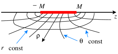
Figure 2: In Weyl coordinates the Schwarzschild black hole is represented as a rod in the $\rho,z$ horizontal half-plane. Lines of constant Schwarzschild coordinates $r$ and $\theta$ are outlined.

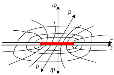
Figure 3: The full Weyl representation of Schwarzschild includes complex $\rho$ values to describe the interior of the horizon and a second copy of the horizontal half-plane.

The Penrose diagram in $t,r$ can be divided into four regions that meet in a $\times$-structure. In Weyl coordinates we also have a similar structure since we can also perform the analytic continuation to a second vertical region $\rho^{\prime}=-i\rho$ and then to a second horizontal region at negative real $\rho$. So we put another copy of the horizontal external universe behind the horizon and another copy of the vertical region below (see Figure 3) for a total of a four card junction similar to the Penrose diagram. The four regions labelled H1, H2, V1 and V2 in

the Penrose diagram map to the similarly labelled region on the card diagram in Fig. 1. Note however that the Weyl cards we are building represent the $r,\theta$ coordinates of the Schwarzschild solution which is different from the Penrose diagram. However the fact that the radial coordinate $r$ describes four distinct regions, two where $\partial_{r}$ is spacelike and two where it is timelike, is still apparent in the Weyl card diagram.

Let us next examine what the (upper) vertical card looks like. Looking at an $r$-orbit on the vertical card, we note that $0\leq\rho^{\prime}\leq M\pm z$. These bounding lines are where we have a zero of $R_{\pm}=\sqrt{-\rho^{\prime 2}+(z\pm M)^{2}}$, which we call special null lines and they are

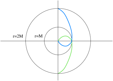
Figure 4: The Weyl null lines for the Schwarzschild black hole correspond to two 3-surfaces whose cross sections are cardioids.

a general feature of vertical cards with focal points (the rod endpoints $z=\pm M$ on the Schwarzschild card). Here the null lines are the envelope of the $r$-orbits as we vary $\theta$. Thus when inside the horizon the BL coordinates apparently fill out a vertical 45-45-90 degree triangle in Weyl coordinates with hypotenuse length $2M$ as shown in Figure 5.

Special null lines play an important role in Weyl card diagrams so let us explain their significance. Keep in mind that we have already broken the manifest spherical symmetry when we have written Schwarzschild in Weyl coordinates, so the existence of preferred special null lines is relative to this chosen axis. In Boyer-Lindquist coordinates, we want to look at the vanishing of

$$R_{\pm}=r-M\pm M\cos\theta.$$ (5)

As drawn in Fig. 4, the 3-surfaces $R_{\pm}=0$ have a cardioid shape. For a given axis there are two, and these surfaces intersect at $r=M$ and partition the inside-horizon into four subregions. These regions will correspond to four triangles which we describe below and the null lines correspond to the above 3-surfaces. At any point in the diagram, two axes may be chosen and cardioids drawn to bound the future trajectories of null or timelike curves.

It is clear from (5) that $R_{\pm}$ is positive outside the horizon and there is no difficulty going to negative values inside the horizon. On the other hand in terms of Weyl coordinates, the functions $R_{\pm}=\sqrt{-\rho^{\prime 2}+(z\pm M)^{2}}$ are the square root of a positive number when $\rho^{\prime}<(z\pm M)$ and the function is imaginary if we naively cross the null line. As we will discuss in more detail, the difficulty in Weyl coordinates is actually that we initially use the positive

branch of the square root, but as the radicand passes through zero, we must switch branches of the square root function. This is just the statement that the function $x\mapsto\sqrt{x^{2}}$ can be continued through $x=0$ to negative values. To obtain a proper Weyl description of the Schwarzschild solution it is necessary to extend the spacetime past the null lines. The resolution is that we may continue to use the coordinates $\rho^{\prime},z$ on the same triangle $0\leq\rho^{\prime}\leq M\pm z$ to describe the interior of the black hole but with two important details. One is that every time though we cross a special null line we change the sign of $R_{+}$ or $R_{-}$ depending on which line we cross. The

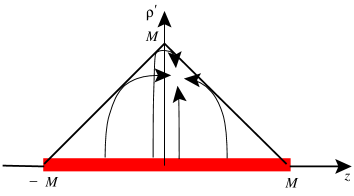
Figure 5: The Weyl representation of the interior of the Schwarzschild black hole naively gives a triangle with base length $2M$ and height $M$. The interior is covered four times by orbits of $r$ at four different values of $\theta$.

second is that the coordinates cover only a portion of the interior and we must properly glue these coordinate patches together to fill out the entire region inside the horizon. So for example the horizon and the singularity are both described as being at $\rho^{\prime}=0$ but the metric near the singularity will have all instances of $R_{\pm}$ replaced by $-R_{\pm}$.

To understand this resolution let us return to the coordinate map. An analysis of Eq. 4 shows that the BL coordinates cover the same triangle four times and we depict this in Figure 5. Of note is the fact that an $r$-orbit which initially is timelike (upward) on the vertical card turns seemingly spacelike (leftward) after touching the special null line, while in fact it should always be timelike. Therefore this naive extrapolation of Weyl coordinates into the horizon is not accurate.

A very simple and visually appealing solution to this problem exists. All difficulties with the coordinates can be fixed by simply unfolding the four copies of the triangle across the special null lines to produce a square of length $2M$. For example this will turn the bottom triangular region on its side as shown in Fig. 7 by the left and right triangles. In addition to extending the coordinates, we must also properly extend the metric across the null lines so the metric in the different triangles corresponds to different spacetime points. The first unfolding, drawn down to $r=M$, is shown in Fig. 6, and the end result with the manifestly timelike $r$-orbits, drawn all the way to $r=0$, is shown in Fig. 7. In the Schwarzschild geometry it is possible to explicitly see that $e^{2\gamma}$ changes sign when we change the overall sign of one of the $R_{\pm}$ in Weyl coordinates. Changing the sign of $e^{2\gamma}$ as we pass the null lines is the way to properly unfold the coordinate triangles because it interchanges which of the the $\rho,z$ coordinates is timelike and which is spacelike. Note that $\gamma$ is therefore not necessarily real and its imaginary part can be either $0$ or $\pi$. Also because of the unfolding of the triangles, the positive $z$-direction on the top triangle horizontal cards points in the opposite direction compared to on the original horizontal card.

Figure 6: To fix the overlap for the region $M\leq r\leq 2M$, we note that each fixed $\theta$ value tangentially intersects the triangle for two specific values of the coordinate $r$. Reflecting about the tangential intersection point on the triangle we fill out a rectangle of height $M$ and width $2M$. This is half the vertical card.

The vertical cards for the Schwarzschild black hole are thus both squares of length $2M$. The bottom of the upper card V1 is the black hole horizon which connects to three other cards in a four card junction. The right and left sides of this vertical card at $\theta=0,\pi$ are boundaries where the $\phi$-circle vanishes. The top edge of the card at $r=0$ is the black hole curvature singularity. Fig. 7 depicts the region $0\leq r\leq 2M$ on the upper vertical card. The second vertical card is build in analogous fashion except the square is built in a downwards fashion towards negative values of $\rho^{\prime}$. Also there is a second horizontal card plane identical to the first attached to the same horizon. We have now described how to build the card diagram for the Schwarzschild black hole in Figure 1.

Figure 7: Unfolding the four triangles for Schwarzschild the Weyl space for the range $r=[0,2M]$ produces a square of length $2M$. The horizon is at the bottom and the singularity at the top.

One would ordinarily stop the construction of Schwarzschild with the above four regions, but for reasons which become more clear when we look at the Reissner-Nordstrøm and Kerr black holes in Sections 5.1.1 and 5.1.4, we continue the spacetime past the singularity to attach two horizontal half-plane corresponding to negative-mass universes, and another vertical card above. In Schwarzschild coordinates, these negative-mass universes represent $r<0$ nakedly singular spacetimes. Each negative mass-universe is one horizontal half-plane card with a singularity along $-M\leq z\leq M$. The total card diagram for Schwarzschild is an infinite stack of cards representing positive and negative mass universes and the inside-horizon regions, shown in Fig. 8.

Figure 8: The extended card diagram for Schwarzschild includes both positive and negative mass universes half-planes. Its side-view for $z=0$ cross-section is drawn on the right.

2.2 General properties of card diagrams

Having described the construction of the card diagram for Schwarzschild we now turn to a few general remarks about these diagrams. Horizontal cards are conformally Euclidean and represent stationary regions. Vertical cards are always conformally Minkowskian and represent regions with ($D-2$) spacelike Killing fields. On a vertical card time is always in the vertical direction and causal cones lie between the $45^{\circ}$ angles. Weyl’s coordinates certainly go bad at horizons, so these diagrams are not a full replacement for Penrose diagrams at understanding causal structure or particle trajectories. However, it is clear for example from Fig. 8 that two vertical and two horizontal cards attach together in a $+$-configuration in precisely the sense of the $\times$-like horizon structure of the Penrose diagram.

The prototypical horizon is that of the two Rindler and two Milne wedges of flat space; this spacetime has two horizontal half-plane cards and two vertical half plane cards that meet along the horizon being the whole $z$-axis. Zooming in on a non-extremal horizon of any card diagram yields this Rindler/Milne picture.

A rod endpoint $(\rho,z)=(0,z_{i})$ such as $z=\pm M$ for Schwarzschild is a ‘focus’ for the Weyl diagram and often represents the end of a black hole or acceleration horizon on a horizontal card. Quite generally, multi-black hole Weyl spacetimes depend only on distances to foci [27].

To understand that it is natural in general to change the branch of the functions $R_{i}$ when crossing the special null line that emanates from the foci at $z=z_{i}$, take some Weyl spacetime and imagine moving upwards in a vertical card to meet the special null line at $R_{i}=0$ by increasing time $\rho^{\prime}\geq 0$ for fixed spatial $z$. Rearranging $R_{i}=\sqrt{-\rho^{\prime 2}+(z+z_{i})^{2}}$ as the semi-ellipse

$$R_{i}^{2}+\rho^{\prime 2}=(z+z_{i})^{2},$$

we see that a smooth traversal of this semi-ellipse across $R_{i}=0$ requires a change in the sign of $R_{i}$.

In many of our solutions, special null lines are used to reflect vertical triangular cards to create full, rectangular cards. However, in the Bonnor-transformed S-dihole II geometry of Sec. 3 as well as double Killing rotated extremal geometries and parabolic representations of the bubble and S-Schwarzschild in Sec.2.3.3, the special null lines will serve as conformal null infinity ${\cal I}^{\pm}$.

Boundaries of cards indicate where Killing circles vanish. Which circle vanishes is constant over a connected piece of the boundary, even when the boundary turns a right angle onto a vertical card. Furthermore the periodicity to eliminate conical singularities is constant along connected parts of the boundary. For the Schwarzschild, the $\phi$-circle vanishes on both the connected boundaries and has periodicity $2\pi$.

When a light ray is incident from a horizontal card onto a horizon (to enter the upper vertical card), it must turn and meet that horizon perpendicularly. It then appears on the vertical card, again perpendicular to the horizon. Only those light rays which go from the lower vertical card to the upper vertical card directly can meet the horizon line at a non-right angle; these rays would touch the vertex of the $\times$ in a Penrose diagram such as in the Schwarzschild case. When a light ray on a vertical card hits a boundary where a spacelike circle vanishes, it bounces back at the same angle as drawn on the card.

Spacetimes with a symmetry group larger than the minimal Weyl symmetry can have more than one card diagram representation. This is due to the fact that there can be more than one way to set up a Killing congruence on the spacetime manifold which is still compatible with the Weyl Ansatz. Examples we explicitly discuss in Sec. 2.3 are the 4d Witten bubble and the 4d S-Reissner-Nordstrøm (S-RN) which have three card diagrams corresponding to the three types of Killing congruences on dS₂ or ${\bf H}_{2}$; Secs. 5.2.4 and 5.2.5 discuss the 5d cases. In comparison both the Schwarzschild and RN black holes have only one card diagram since on the sphere $S^{2}$, all Killing congruences are axial rotations and lead to the same card diagram. The S-Kerr solution of Sec. 5.1.4 has symmetry group $U(1)\times{\bf R}$ so it also has only one representation, which looks like the ‘elliptic’ representation of S-RN. The multiple representations of the Witten bubble echo the fact that dS₂ can be represented in different Killing coordinate systems. Using hyperbolic and trigonometric functions, two types of congruences are easy to find; one of them is associated with global coordinates, while the other has patched coordinates. Different representations have different uses. For example the patched Witten bubble can be trivially Wick rotated to give the Schwarzschild black hole or the S-Schwarzschild, whereas when the bubble is written in global coordinates more work is required in order to obtain these other spacetimes in Weyl coordinates (see Sec. 5.2.2).

2.2.1 Our deck of cards: The building blocks for Weyl spacetimes

All spacetimes, new and old, in this paper are built from the following card types.

Horizontal cards are always half-planes. They may however have one or more branch cuts which may be taken to run perpendicular to the $z$-axis. Undoing one branch cut leads to a strip with two boundaries; multiple branch cuts lead to some open subset, with boundary, of a Riemann surface.

Vertical cards can be half-planes with a vertical boundary, half-planes with a horizontal (horizon) boundary; quarter-planes with a vertical and horizontal boundary and one special null line; compact squares with two special null lines; a full plane with two special null lines; a full plane without special null lines; a noncompact $45^{\circ}$ wedge with either a vertical or horizontal boundary, and a special null line serving as conformal null infinity ${\cal I}^{\pm}$; a compact $45$-$45$-$90$ wedge with the hypotenuse either vertical or horizontal, and short legs being special null lines serving as ${\cal I}^{\pm}$; a noncompact $90^{\circ}$ wedge bounded by two ${\cal I}^{\pm}$ special null lines; and a compact $45$-$45$-$90$ wedge with hypotenuse serving as ${\cal I}^{\pm}$, and legs horizontal and vertical.

It is satisfying that for a variety of spacetimes, the cards are always of the above rigid types.

There is one basic procedure which can be performed on vertical cards and their corresponding Weyl solutions. It is the analytic continuation $\gamma\to\gamma+i\pi$, which is allowed since $\gamma$ is determined by first order PDEs. This continuation is equivalent to multiplying the metric by a minus sign and then analytically continuing the $D-2$ Killing directions. We call this a $\gamma$-flip since the way it acts on a card is to mirror-reflect it about a $45^{\circ}$ null line (for example, look at the vertical cards in Figs. 12 and 12). Our first example of this procedure as generating a new solution appears in (15).

2.3 Witten bubble and Schwarzschild S-brane

The Schwarzschild black hole can be analytically continued to two different time dependent geometries, the Witten bubble of nothing[2] and S-Schwarzschild[15, 16, 17], and it is instructive to understand how the card diagram changes.

One of the main new features that arises is that a spacetime can have multiple card diagram representations. Both the bubble and S-Schwarzschild have three different card diagram representations corresponding to three different ways to select Killing congruences. Analyzing the different diagrams we also find that analytic continuations have a very simple form in Weyl space allowing us to relate them in a visually satisfying manner.

We will discuss these different representations in detail when constructing the card diagrams. To set the stage, however, we make some preliminary remarks on the symmetries of hyperbolic spaces. These three types of Killing congruences can be understood directly by representing ${\bf H}_{2}$ as the unit disk (with its conformal infinity being the unit circle). The orientation-preserving isometries of ${\bf H}_{2}$ are those Möbius transformations preserving the disk, $PSL(2,{\bf R})$ [28]. Möbius transformations $z\mapsto{az+b\over cz+d}$ have two complex fixed points, counted according to multiplicity. In the upper half-plane $z=x+i\sigma$ representation, $a$, $b$, $c$, and $d$ are real, so the fixed points are roots of a real quadratic. Hence they may be (i) distinct on the real boundary (hyperbolic), (ii) degenerate on the real boundary (parabolic), or (iii) nonreal complex conjugate pairs, one interior to the upper half plane ${\bf H}_{2}$ (elliptic). Prototypes of Killing fields are (i) $z\to(1+\epsilon)z$ for the upper half-plane, (ii) $z\to z+\epsilon$ for the upper half-plane; and (iii) $z\to e^{i\epsilon}z$ for the disk $|z|<1$. These are the striped, Poincaré, and azimuthal congruences. In these representations, the S-Reissner Nordstrom (S-RN) and the Witten bubble each have 0, 1, and 2 Weyl foci.

2.3.1 Hyperbolic card diagrams

Originally Witten found the expanding bubble solution by starting from (2) and taking the analytic continuation $\theta\to\pi/2+i\theta$ and $t\to ix^{4}$

$$ds^{2}=(1-2M/r)(dx^{4})^{2}+(1-2M/r)^{-1}dr^{2}-r^{2}d\theta^{2}+r^{2}\cosh^{2}\theta\,d\phi^{2}.$$ (6)

Here, $\theta$ plays the role of time and $\theta=0$ is the time where the bubble ‘has minimum size.’ (This statement has meaning if we break $SO(2,1)$ symmetry.) To achieve this in Weyl’s coordinates, we put $z\to i\tau$, $t\to ix^{4}$; the resulting space is equivalent to Witten’s bubble by the real coordinate transformation

$$\rho = \sqrt{r^{2}-2Mr}\,\cosh\theta$$

$$\tau = (r-M)\sinh\theta.$$

Witten’s bubble universe is represented in Weyl coordinates as a vertical half-plane card, $\rho\geq 0$, $-\infty<\tau<\infty$, where now the $x^{4}$-circle, and not the $\phi$-circle, vanishes at $\rho=0$. Note that the vertical card now has Minkowski signature and is conformal to $-d\tau^{2}+d\rho^{2}$. This vertical card does not have special null lines and is covered only once by the BL coordinates. The bubble does have a rod which is along the imaginary $\tau$ axis and which intersects the card at the $\rho=0$, $\tau=0$ origin. The reason there are no special null lines is that the geometry’s foci are at $\tau=\pm iM$. We call this the hyperbolic representation of the Witten bubble.

This analytic continuation in Weyl space is precisely the same as the one used in [19], except now the Schwarzschild rod crosses $z=0$. Solutions which are even-in-$z$ Israel-Khan arrays where no rod crosses $z=0$ can be Wick rotated to gravitational wave solutions sourced by rods at imaginary time. Generalizations of the bubble solution by adding concentric incoming and outgoing waves include Wick rotations of an Israel-Khan array even about $z=0$ where one rod does cross $z=0$. As these additional rods are made to cover more of the $z$-axis and are brought closer and closer to the principal rod, the deformed Witten bubble solution hangs longer with a minimum-radius $\phi$-circle. In the limit where rods occupy the entire $z$-axis, we get a static flat solution, which is Minkowski 3-space times a fixed-circumference $\phi$-circle.

It is well known that sending $t\to ix^{4}$, $\phi\to i\phi$ gives another, ‘elliptic’ representation of the Witten bubble (see Fig. 9). We will discuss this in the next subsection. However, sending $t\to ix^{4}$ and $\phi\to i\phi$ for a finite Israel-Khan array [4, 29] yields a solution different than sending $z\to i\tau$; we get black holes and conical singularities in an expanding Witten bubble. We see that to smoothly perturb the Witten bubble by adding more sources at imaginary time, the use of Weyl’s coordinates and $z\to i\tau$ is essential.

The Schwarzschild S-brane vacuum solution of [15, 16, 17]

$$ds^{2}=(1-2M/t)(dx^{4})^{2}-(1-2M/t)^{-1}dt^{2}+t^{2}(d\theta^{2}+\sinh^{2}\theta d\phi^{2})$$ (7)

is gotten from (2) by taking $t\to ix^{4}$, $\theta\to i\theta$, $r\to it$, and $M\to iM$. From (3) we see that in Weyl’s coordinates we can effect this by sending $t\to ix^{4}$, $z\to i\tau$, $M\to iM$, up to a real coordinate transformation. Thus in Weyl coordinates the only difference between Witten’s bubble and the Schwarzschild S-brane is putting $M\to iM$. In the terminology we are using, a hyperbolic representation of the Witten bubble becomes an elliptic representation of S-Schwarzschild (see the next section) under the analytic continuation of the mass.

We can also take the Witten bubble in the hyperbolic representation and turn the vertical half-plane card on its side via $\gamma\to\gamma+i\pi$. This yields a hyperbolic representation of S-Schwarzschild which we will leave for Sec. 5.2.2 because the horizontal card has an interior branch point which is more technically involved.

Just as we perturbed Witten’s bubble solution with an Israel-Khan array, we can also perturb S-Schwarzschild by adding rods before analytically continuing. Here Weyl’s coordinates and $z\to i\tau$ are essential. We can choose to analytically continue the mass parameters of the additional rods or not. Additionally, we can displace some rods in the imaginary $z$-direction which affects the $\tau$-center of their disturbance. If we do everything in an even fashion, i.e. we respect ${\rm Im}\,\tau\to-{\rm Im}\,\tau$, the resulting geometry (at real $\tau$) will be real. In particular, rotating a rod at $z>0$ counterclockwise means rotating its image at $z<0$ clockwise. We will see in Sec. 5.3.1 in reinvestigating the 2-rod example [19] that there may be several choices for branches.

2.3.2 Elliptic card diagrams

Weyl solutions can have multiple card diagram representations and we illustrate this by first discussing the elliptic card diagram for the Witten bubble. Starting with Schwarzschild and sending $z\to i\tau$ and $t\to ix^{4}$ gives the Witten bubble with a single vertical half-plane card $\rho\geq 0$, $-\infty<\tau<\infty$. However, one can also take Schwarzschild and send $t\to ix^{4}$ and $\phi\to i\phi$ and the metric on the two sphere becomes two dimensional de Sitter space $d\theta^{2}-\sin^{2}\theta d\phi^{2}$. Now $\phi$ is a timelike coordinate and we leave it noncompact. At $\theta=0,\pi$ there are clearly Rindler type horizons about which we analytically continue $\theta$ and again obtain de Sitter space $-d\theta^{2}+\sinh^{2}\theta d\phi^{2}$.

This second analytic continuation to the Witten bubble in Schwarzschild coordinates

$$ds^{2}=(1-2M/r)(dx^{4})^{2}+(1-2M/r)^{-1}dr^{2}+r^{2}(d\theta^{2}-\sin^{2}\theta d\phi^{2})$$ (8)

has a corresponding second analytic continuation in Weyl coordinates. In Weyl coordinates we find that analytically continuing the time $t$ turns the horizon of the Schwarzschild card into a boundary, while continuing the coordinate $\phi$ turns the boundaries on the horizontal card into noncompact acceleration horizons along the semi-lines $|z|\geq M$, $\rho=0$; the coordinate $z$ is not continued. Setting $\rho^{\prime}=i\rho$ at the horizons, we find a vertical 45 degree triangular cards with special null lines on the semi-infinite rays $\rho^{\prime}=z-M$ for $z\geq M$ and $\rho^{\prime}=-M-z$ for $z\leq-M$. This region is doubly covered and so it is necessary to change branches of the function $R_{\pm}$ at the null line as in the Schwarzschild case and this procedure produces a quarter-plane vertical card. These null lines are extensions of the null lines of the Schwarzschild solution onto the bubble card diagram. From the BL coordinate point of view they lie on $r=M+M\cosh\theta$ which extends outward to large values of $r$. The two horizontal half-plane cards are static patches of the solution. This elliptic card representation of the Witten bubble is shown in Fig. 9.

This second card diagram of the Witten bubble is closely related to the Schwarzschild card we previously constructed. In the language of [4], there are actually both $e^{2U_{1}}$ rods which exist for the coordinate $t$, as well as $e^{2U_{2}}$ rods for $\phi$. Double Killing rotation (analytic continuation) of the coordinates $t$ and $\phi$ is equivalent to switching which Killing coordinate each rod sources. Hence the elliptic representation of the Witten bubble is sourced by two semi-infinite (time) rods separated by a ($\phi$) line segment rod. This is an alternate view of the construction of the elliptic card diagram for the Witten bubble.

Figure 9: The elliptic representation of the Witten bubble contains two horizons and four special null lines.

In this representation, one has the freedom to identify the rear horizontal cards gotten to by going through the left and right acceleration horizons. We may also identify after a finite number of trips around; this gives a discrete set of spacelike periodicities of dS₂. In the hyperbolic representation (one vertical card), the azimuth of dS₂ was not drawn and we were free to make any periodicity. On the other hand the elliptic representation makes clear that someone in the right vertical card is causally disconnected from someone in the left vertical card. Different card diagram representations highlight different features and possibilities.

The reason that more than one card diagram exists for the same solution can be thought of as different ways to setup a Killing congruence on our symmetric space. For the case of the Witten bubble the symmetric space is dS₂ and for S-Schwarzschild it is ${\bf H}_{2}$.

The symmetry of the bubble solution is large enough so that we may write the bubble in Weyl coordinates in three distinct ways which allow us to see different parts of the symmetry structure. The two aforementioned hyperbolic and elliptic representations of the bubble are easily understood by examining the embedding of dS₂ into flat space.

To begin with, the unit sphere

$$ds^{2}=d\theta^{2}+\cos^{2}\theta d\phi^{2}$$ (9)

has an $SO(3)$ symmetry and may be embedded into ${\bf R}^{3}$ as

$$Z=\sin\theta,\ X=\cos\theta\cos\phi,\ Y=\cos\theta\sin\phi,\qquad Z^{2}+X^{2}+Y^{2}=1.$$ (10)

The sphere can be analytically continued to global coordinates covering all of de Sitter space by taking $\theta\rightarrow i\theta$, which sends $Z\to iZ^{\prime}$, and so we now have an embedding into ${\bf R}^{2,1}$

$$Z^{\prime}=\sinh\theta,\ X=\cosh\theta\cos\phi,\ Y=\cosh\theta\sin\phi,\qquad-Z^{\prime 2}+X^{2}+Y^{2}=1$$ (11)

$$ds^{2}=-d\theta^{2}+\cosh^{2}\theta d\phi^{2}\ .$$ (12)

The coordinate $\phi$ parametrizes the azimuthal angular direction whose periodicity we may choose. This gives the first hyperbolic representation of the bubble.

It is also possible to obtain by analytic continuation a second embedding of de Sitter by $\phi\rightarrow i\phi$, so $Y\to iY^{\prime}$

$$Z=\sin\theta,\ X=\cos\theta\cosh\phi,\ Y^{\prime}=\cos\theta\sinh\phi,\qquad Z^{2}+X^{2}-Y^{\prime 2}=1$$ (13)

$$ds^{2}=d\theta^{2}-\cos^{2}\theta d\phi^{2}\ .$$ (14)

In this case the coordinate $\phi$ now parametrizes a noncompact direction. This embedding gives only a patch $|Z|\leq 1$, $X\geq 0$ of de Sitter. Our elliptic representation of the bubble comes from this second analytic continuation. Both of these two analytic continuations give de Sitter space with $SO(2,1)$ symmetry but in different parametrizations and this is reflected in the two card diagrams.

Now let us turn to the ‘elliptic’ construction of S-Schwarzschild (7), which is a vertical $\rho,\tau$ card, but the metric is only real for $0\leq\rho\leq\tau-M$ (or for the equivalent region $0\leq\rho\leq-\tau-M$). The boundary $\rho=\tau-M$ is a special null line; in BL coordinates the null lines are $R_{\pm}=t-M\pm M\cosh\theta=0$. This triangular region is covered twice and so we flip the triangular region about the null line to make a quarter-plane vertical card. A null line appears for the S-brane solution because the focus of Schwarzschild at $z=M$ continues to $\tau=M$ which is on the real manifold; special null lines always extend at $45^{\circ}$ on vertical cards, from foci on the real manifold. Since we have analytically continued coordinates, the null line now extends to large values of time. In Weyl coordinates these null lines are simply the vanishing of $R_{\pm}$ which is a function of say complexified $\rho,\tau$; (S-)Schwarzschild and the Witten bubble have null lines each being a real section of the same complex locus.

The vertical boundary is at $\theta=0$ where the $\phi$-circle vanishes. We then pass down through the lower edge $x^{4}$-horizon to a horizontal $\rho^{\prime},\tau$ half-plane card. The full card diagram is like the elliptic Witten bubble of Fig. 9, except the $\phi$-circle vanishes on the boundary, and there is a singularity at the intersection of horizontal and vertical cards on the left side; note that the coordinate labels $\rho$ and $\rho^{\prime}$ should be interchanged (as in Fig. 26 which is the charged version of this solution). Just like for the Schwarzschild black hole card diagram, past the singularity we have attached negative mass universes which are represented as quarter plane vertical cards, for reasons which become more clear when looking at charged solutions.

Note how the card representation of the S-brane is quite different from the black hole card diagram while the Penrose diagrams are related by a simple ninety degree rotation. This is because the card diagram shows the compact or noncompact $\theta$ direction, which shows the distance from the S-brane worldvolume.

There is an alternate way to get (elliptic) S-Schwarzschild from the elliptic representation of the Witten bubble. Take the vertical card and perform a $\gamma$-flip by sending $\gamma\to\gamma+i\pi$. This turns a vertical card on its side, interchanging the Weyl spacelike and timelike coordinates. Performing this operation on the Witten bubble’s vertical quarter plane card with its $x^{4}$-boundary and $\phi$-horizon, results in the S-Schwarzschild’s vertical quarter plane card with a $\phi$-boundary and $x^{4}$-horizon as described above. Continuing through the four card junction horizon, we fill out the rest of S-Schwarzschild. In terms of Schwarzschild coordinates this $\gamma$-flip amounts to starting with the Witten bubble and changing the signs for $g_{rr}$ and $g_{\theta\theta}$

$$(1-\frac{2M}{r})(dx^{4})^{2}+\frac{dr^{2}}{1-\frac{2M}{r}}+r^{2}(-d\theta^{2}+\sinh^{2}\theta d\phi^{2})$$ (15)

$$\qquad\longrightarrow(1-\frac{2M}{r})(dx^{4})^{2}-\frac{dr^{2}}{1-\frac{2M}{r}}+r^{2}(d\theta^{2}+\sinh^{2}\theta d\phi^{2})$$

to obtain the S-Schwarzschild solution.

The elliptic form of the card diagrams show that Schwarzschild S-brane, Witten bubble and Schwarzschild solutions have similar structures and in fact they are all related by $\gamma$-flips and trivial Killing continuations. Solutions which are related in this manner may be conveniently drawn together in one diagram which simultaneously displays all of their card diagrams. For example in the diagram in Fig. 10 the S-Schwarzschild solution comprises regions $1,2,3,4,5$, the Witten bubble is regions $4,5,6$ and the Schwarzschild black hole is $6,7,8,9,10$. Regions $1,2,10$ correspond to a singular Witten bubble of negative ‘mass.’ For example on the Schwarzschild card the horizontal card is region 6 and the vertical card square is regions 7,8 and 9, while region 10 is the negative mass horizontal card; note that this diagram represents all the different types of card which appear in the full Schwarzschild card although not every card in the infinite extended diagram. In this diagram we also see that the special null lines extend through the individual solutions and so are a feature of the complexified spacetime.

Figure 10: The Schwarzschild black hole, Witten bubble and S-Schwarzschild are all related by $\gamma$-flips and so their card diagrams may be combined into this one extended diagram.

2.3.3 The parabolic diagram: Poincaré time

There is a third way to put a Killing congruence on ${\bf H}_{2}$ or dS₂ using Poincaré coordinates. Parametrizing hyperbolic space (which is just Euclideanized AdS₂) as $ds^{2}=\sigma^{2}dx^{2}+{d\sigma^{2}\over\sigma^{2}}$, and keeping the BL coordinate $t$ and the usual $x^{4}$ we get a Poincaré Weyl representation of the S-Reissner-Nordstrøm (S-RN) spacetime[3, 15, 16]. This is a charged version of the S-Schwarzschild where the $t$ dependence is governed by $t^{2}-2Mt-Q^{2}$ with zeroes $t_{+}>0$, $t_{-}<0$, and a singularity at $t=0$. The charged S-brane is

$$ds^{2} = f(dx^{4})^{2}-f^{-1}(e^{2\gamma}(-d\rho^{\prime 2}+dz^{2})+\rho^{\prime 2}dx^{2}),$$

$$A = Qdx^{4}/t,$$

$$f = (1-2M/t-Q^{2}/t^{2}),$$

$$e^{2\gamma} = {t^{2}-2Mt-Q^{2}\over\sigma^{2}(M^{2}+Q^{2})},$$

$$\rho^{\prime} = \sigma\sqrt{t^{2}-2Mt-Q^{2}},$$

$$z = \sigma(t-M).$$

In this Weyl representation, $\rho^{\prime}$ is timelike on a $t>t_{+}$ vertical card which is a noncompact $45^{\circ}$ wedge, $\rho^{\prime}<|z|$. This connects along $z>0$ to a $t_{-}<t<t_{+}$ horizontal card; a $t<t_{-}$ vertical card attaches to $z<0$. So this is similar to the representation of S-RN (or S-Schwarzschild) that we have seen, except the line segment $-M<z<M$ has collapsed and the special null lines are now conformal null infinity (Fig. 12). The singularity on the horizontal card is particularly easy to describe in these coordinates; it is on a ray $z/\rho=-M/Q$. For comparison, the elliptic and hyperbolic representations are in Figs. 26 and 27.

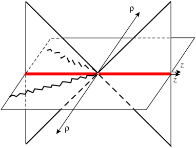
Figure 11: The parabolic card diagram representation for S-Reissner Nordstrom. The forty five degree vertical lines represent null infinity.

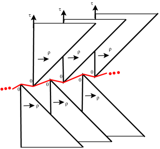
Figure 12: The parabolic representation of the Witten bubble contains an infinite number of wedge vertical cards pointing up and down with each wedge joined to two others at the tip in a dS₂ fashion.

If we take the $t>t_{+}$ (or $t<t_{-}$) $45^{\circ}$ wedges and turn them on their sides via $\gamma\to\gamma+i\pi$, we get the parabolic version of the $r\geq r_{+}$ charged Witten bubble. The line which used to be the horizon in the S-brane card diagram becomes a boundary which is the minimum volume sphere, at $\rho=0$. Time is now purely along the $\tau$ direction as in the hyperbolic bubble card representation. The special null line is still ${\cal I}^{\pm}$ since $\rho=|\tau|$ corresponds to $r\to\infty$. The vertex of the card is not the end of the spacetime. These wedge cards only represent $\sigma>0$ and so the card diagram should be extended to negative times. The card diagram is an infinite row of $45^{\circ}$ wedge cards pointing up and an infinite number pointing down. The vertex of each upward card is attached to its nearest two downward neighbors (one to the left and one to the right), in the usual dS₂ fashion as shown in Figure 12. One can identify cards so only needs one upward and one downward card with two attachments. Although this card diagram is not the most obvious representation of the Witten bubble, it will be useful in understanding the more complicated S-dihole II universes of Sec. 3.

2.4 Gravitational wave fall-off

The Schwarzschild S-brane (7) has a warp factor for the brane direction of $1-2M/t$, which decays to unity as $1/t$. This is the expected behavior at fixed spatial position for a wave produced by a $(2+1)$-codimension source. To really consider the wave equation, we should move to conformally Minkowskian coordinates in two dimensions, Weyl coordinates $(\rho,\tau)$, and follow the wave as it propagates outward at the speed of light. As we have seen, the S-Schwarzschild geometry includes such a vertical card region with some outgoing wave activity centered about $\rho=\tau+M$. As $t\to\infty$ along this null line, $\rho\sim t^{2}/M$, and so our wave falls off as $1/\tau^{1/2}$. This is the same fall-off as the warp factor for the S-dihole of [19].

We can understand this power-law decay with the following simplified model, using $x,y,z,\tau$ coordinates in Minkowski 4-space. A codimension $3+1$ source for the wave equation gives precisely causal wave fronts, and a codimension $2+1$ source can be gotten by dimensional reduction. Hence we may write a wave as

$$\Psi(x,y,\tau)=\int_{-\infty}^{\infty}\Big{(}{dz\over x^{2}+y^{2}+z^{2}-\tau^{2}+i\epsilon}+{\rm c.c.}\Big{)}$$

where $\epsilon$ is a regulator. Along $x^{2}+y^{2}-\tau^{2}=0$, $\Psi={1\over\sqrt{\epsilon}}\int_{-\infty}^{\infty}{\zeta^{2}d\zeta\over\zeta^{4}+1}$. If the wave is regulated by displacing the source into imaginary time, $\tau\to\tau-ia$, we find that $\epsilon\propto\tau$. Therefore the behavior for such time-displaced wave sources is $\Psi\sim 1/\tau^{1/2}$ and this is precisely the case for the S-dihole of [19]. In the S-Schwarzschild case, the card diagram is more complicated and the singularity is stationary, but we expect a similar fall off of the metric along the vertical card.

3 New S-branes from Diholes

In this section we discuss new time dependent solutions which arise by analytically continuing dihole solutions. The use of Weyl coordinates and the construction of card diagrams will be helpful in understanding their interesting global structure. We first review the dihole solution as well as the S-dihole solution of [19] before examining new S-dihole solutions.

The extremal black dihole of [20, 30, 21] was analytically continued [19] to obtain a smooth time dependent solution free of curvature singularities, closed timelike curves (CTCs) and horizons. Let us refer to that solution as S-dihole I. In the previous section, we discussed how in Weyl coordinates the Schwarzschild solution may be analytically continued to the bubble of nothing and if we additionally send $M\to iM$ this gives us the S0-brane solution which we called S-Schwarzschild.

Many gravity solutions can be analytically continued to obtain new time dependent spacetimes and it is not uncommon to have two or more different analytic continuations. Sending the mass parameter $M\to iM$ in Weyl coordinates for the S-dihole I solution produces a substantially different S-dihole II. One of the main differences for spacetime structure, is that the Weyl foci and the special null lines are at real values and so will play an important role. These new solutions are related to the decay of unstable objects, cosmological solutions [22] and posses near horizon scaling limits.

3.1 Diholes, S-diholes and Bonnor transformations

The black magnetic dihole metric in Boyer-Lindquist coordinates (assuming $a\neq 0$) is

$$ds^{2}=(1-\frac{2Mr}{\Sigma})^{2}[-dt^{2}+\frac{\Sigma^{4}}{(\Delta+(a^{2}+M^{2})\sin^{2}\theta)^{3}}(\frac{dr^{2}}{\Delta}+d\theta^{2})]+\frac{\Delta\sin^{2}\theta}{(1-\frac{2Mr}{\Sigma})^{2}}d\phi^{2}$$ (16)

$$A=\frac{2aMr\sin^{2}\theta}{\Delta+a^{2}\sin^{2}\theta}d\phi$$ (17)

$$\Delta=r^{2}-2Mr-a^{2},\hskip 21.68121pt\Sigma=r^{2}-a^{2}\cos^{2}\theta\ .$$ (18)

The dihole represents two oppositely charged magnetic black holes separated by the coordinate distance $2\sqrt{M^{2}+a^{2}}$ along the $z$-axis.

The dihole was first found using a solution generating technique called the Bonnor transformation starting from the Kerr black hole [20, 31]. In Weyl-Papapetrou coordinates this Bonnor transformation takes a stationary vacuum solution

$$ds^{2}=-f(dt-\omega d\phi)^{2}+f^{-1}(e^{2\gamma}(d\rho^{2}+dz^{2})+\rho^{2}d\phi^{2}),$$

and produces a static charged solution

$$ds^{2} = -f^{2}dt^{2}+f^{-2}(e^{8\gamma}(d\rho^{2}+dz^{2})+\rho^{2}d\phi^{2}),$$ (19)

$$A = B(\rho,z)d\phi,$$

where $\omega=iB$ and $\omega$ is proportional to a parameter (the angular momentum $a$ in the case of Kerr) which must be analytically continued to make $B$ real.

Analytically continuing the coordinates

$$\theta\rightarrow\ \frac{\pi}{2}+i\theta,\ t\rightarrow ix^{4}$$ (20)

gives us the S-dihole I solution of [19]

$$\Delta\rightarrow r^{2}-2Mr-a^{2}=\Delta,\hskip 21.68121pt\Sigma\rightarrow r^{2}+a^{2}\sinh^{2}\theta=\Sigma,$$ (21)

$$ds^{2}=(1-\frac{2Mr}{\Sigma})^{2}[(dx^{4})^{2}+\frac{\Sigma^{4}}{(\Delta+(a^{2}+M^{2})\cosh^{2}\theta)^{3}}(\frac{dr^{2}}{\Delta}-d\theta^{2})]+\frac{\Delta\cosh^{2}\theta}{(1-\frac{2Mr}{\Sigma})^{2}}d\phi^{2}$$ (22)

$$A=\frac{2aMr\cosh^{2}\theta}{\Delta+a^{2}\cosh^{2}\theta}d\phi\ .$$ (23)

This analytic continuation is the same as the one performed on Schwarzschild to obtain the Witten bubble of nothing in the first global representation. The dihole and S-dihole I do not have closed timelike curves in $\phi$, since $r=r_{+,-}$ ($\Delta=0$) is like the origin of polar coordinates and closes off the spacetime. The fact that spacetime stops at $\Delta=0$ and periodically identifying $\phi\simeq\phi+2\pi{a^{4}\over(M^{2}+a^{2})^{2}}$, ensures that the metric and vector potential are well behaved and smooth everywhere.

Bonnor transformations and Wick rotations are both sensible ways to act on the Kerr solution, and it is interesting to consider the set of solutions which can be obtained from their combined effects. Since the dihole is the Bonnor dual of the Kerr black hole, this means that S-dihole I is the Bonnor dual of the Kerr bubble[32, 33]. The Kerr bubble is obtained from Kerr by sending $z\to i\tau$ and $a\to ia$. Although the Kerr bubble needs a twisting to close a circle at the boundary $\rho=0$, we will still consider S-dihole I and the Kerr bubble to be Bonnor dual. S-dihole I was originally defined to be the spacetime where $r\geq r_{+}$. In addition to the spacetime connected to large value of the radius, in these BL coordinates it is clear that S-dihole I actually contains a second non-singular universe where $r\leq r_{-}$; the singularities (surrounding the negative-mass black holes) do not intersect $z=0$ by symmetry. In fact the Kerr bubble is similarly well defined and non-singular for negative values of the radius $r\leq r_{-}$.

Recently the S-Kerr or twisted S-brane solution has been found [24, 25, 26] and we now examine its Bonnor dual which we call S-dihole II. To obtain S-dihole II we analytically continue the dihole in the following alternative method

$$r\rightarrow it,\hskip 21.68121ptt\rightarrow ix^{4},\hskip 21.68121pt\theta\rightarrow i\theta;\hskip 21.68121ptM\rightarrow iM.$$ (24)

The angular momentum is not Wick rotated; it has already been Wick rotated in the Bonnor transformation of Kerr. The S-dihole II solution is

$$\Delta\rightarrow-t^{2}+2Mt-a^{2}=-\Delta,\hskip 21.68121pt\Sigma\rightarrow-t^{2}-a^{2}\cosh^{2}\theta=-\Sigma,$$ (25)

$$ds^{2}=(1-\frac{2Mt}{\Sigma})^{2}[(dx^{4})^{2}+\frac{\Sigma^{4}}{(\Delta+(a^{2}-M^{2})\sinh^{2}\theta)^{3}}(-\frac{dt^{2}}{\Delta}+d\theta^{2})]+\frac{\Delta\sinh^{2}\theta}{(1-\frac{2Mt}{\Sigma})^{2}}d\phi^{2}$$ (26)

$$A=\frac{2aMt\sinh^{2}\theta}{\Delta+a^{2}\sinh^{2}\theta}d\phi.$$

The factor $\Sigma$ is always positive. Remembering that elliptic S-Schwarzschild is more complicated than the hyperbolic Witten bubble, it might be expected that S-dihole II is more complicated than S-dihole I. In fact S-dihole II does have several new and unexpected features. We discuss the properties of this new solution on a case-by-case basis, discuss relevant regions and then discuss how certain regions must be pieced together.

3.2 Extremal case

Let us first examine the extremal case $|M|=|a|$ for S-dihole II. The metric near the origin is

$$ds^{2}={T^{4}\over M^{4}}(dx^{4})^{2}-{M^{4}\over T^{4}}dT^{2}+{M^{4}\over T^{2}}(d\theta^{2}+\sinh^{2}\theta d\phi^{2})$$

C where $T=t-M$. We do not find a de Sitter space limit but a singular metric This extremal case is not related to de Sitter space because the Bonnor transformation has shifted the powers of the coordinate $T$ in the metric components.

3.3 Superextremal case

For the superextremal case $|M|<|a|$, $\Delta$ is never zero and the solution is smooth. The coordinate $\theta$ is noncompact and spacelike. The $\phi$-circle vanishes along $\theta=0$ around which the metric has the expansion

$$ds^{2}\supset{(t^{2}+a^{2})^{2}\over\Delta}(d\theta^{2}+\theta^{2}d\phi^{2})\ .$$

The possible conical singularity can be simply removed by taking $\phi\simeq\phi+2\pi$; this is the same periodicity for the black dihole on the axis outside the black holes.

The superextremal S-dihole II solution is the smooth magnetic Bonnor dual of the superextremal S-Kerr [24]. Both superextremal solutions can be represented by one vertical half-plane card where the edge of the card is a vertical boundary.

3.4 Subextremal case

For the parameter range $|a|<|M|$, S-dihole II has several interesting surprises. This solution can be divided into three separate nonsingular spacetimes and three separate spacetimes with singularities behind acceleration horizons. Some of these spacetimes have near horizon scaling limits and are free of closed timelike curves in four dimensions. To begin with we outline some of their most important features before giving a detailed analysis.

The metric has three coordinate singularities. First, the quantity $(\Delta+(a^{2}-M^{2})\sinh^{2}\theta)^{3}$ in the denominator vanishes at $t^{\rm DH}_{\pm}=M\pm\cosh\theta\sqrt{M^{2}-a^{2}}$. This is an extended analog of the extremal dihole horizons and it is a special null line which serves as null infinity. Second, the factor $\Delta=0$ vanishes when $t^{\rm KH}_{\pm}=M\pm\sqrt{M^{2}-a^{2}}$. In analogy to the Kerr horizon this will turn out to be a Weyl card boundary or horizon. Third, the quantity $\Sigma-2Mt=\Delta+a^{2}\sinh^{2}\theta$ vanishes for small enough $\theta$ $t^{\rm ergo}_{\pm}=M\pm\sqrt{M^{2}-a^{2}\cosh^{2}\theta}$; this is the analog of the Kerr ergosphere. In the case of Kerr, the ergosphere lies between the two Kerr horizons and can be smoothly traversed. For the S-dihole II this Bonnor dual analogue of the ergosphere turns out to be the location of a charged object and is a true singularity. We will continue to use the terminology ‘ergosphere’ for this singular locus.

Due to the three coordinate singularities, it is natural at first glance to consider S-dihole II to be a single solution subdivided into five regions I_±, II_±, and III as indicated on Figure 14.

In regions I₊ and I_-, the coordinate $\theta$ is spacelike, $t$ is timelike and $\theta=0$ is a boundary. This spacetime is smooth and does not have a conical singularity at the boundary if $\phi\simeq\phi+2\pi$.

In regions II₊ and II_-, the coordinate $\theta$ timelike and $t$ spacelike and $t_{\pm}^{\rm KH}$ is thus a boundary where the $\phi$-circle closes. Near $t^{\rm KH}_{+}$ the metric looks like

$$ds^{2}\supset{2\Sigma^{2}\over\sinh^{2}\theta}\left[{a^{4}\over(M^{2}-a^{2})^{7/2}}d\epsilon^{2}+\epsilon^{2}{(M^{2}-a^{2})^{1/2}\over a^{4}}d\phi^{2}\right]\ .$$

where we have made the change of variables $T=t-t^{\rm KH}_{+}=\epsilon^{2}$. To avoid a conical singularity the $\phi$ coordinate has periodicity

$$\phi\simeq\phi+2\pi a^{4}/(M^{2}-a^{2})^{2}\ .$$ (27)

This is the same periodicity in the black dihole which removes the strut from between the black holes [21][19], with the mass $M$ analytically continued.

Region III is therefore separated from regions II_± and has signature $(1,3)$ with $t$, $\theta$, and $\phi$ all being timelike coordinates. To interpret this as a solution to the Einstein-Maxwell equations we perform the $\gamma\to\gamma+i\pi$ flip so the coordinates $t$ and $\theta$ become spacelike leaving just $\phi$ as time; we still label the region after the $\gamma$ flip as region III. See Figure 14. Although this is therefore strictly speaking a new solution we will continue to refer to it as part of S-dihole II. There is a singularity at $t^{\rm ergo}$ which divides this region into an internal small $\theta$ region and an external large $\theta$ part. At this ergosphere, the electric gauge field is infinite and so this is the location of a brane object. The region outside the ergosphere has two horizons, at $t_{\pm}^{\rm KH}$, with Euclidean periodicity (27). Applying the $\gamma$-flip to region III, has turned $t_{\pm}^{\rm KH}$ into horizons which can be traversed. The horizons connect to regions II_± which have also been turned on their side via $\gamma\to\gamma+i\pi$; we will continue to call these region II_±. The internal part has a horizon at $\theta=0$ with Euclidean periodicity $2\pi$. Past this horizon at $\theta=0$ is the new region IV as shown in Fig. 14. Region IV is compact and bounded in these BL coordinates. In fact this boundary is the continuation of $t_{\pm}^{\rm DH}$ and will again represent null infinity!

In the next subsection we provide a full description of these spacetimes and further general discussion of these different regions of the S-dihole II appears in Sec. 3.4.2.

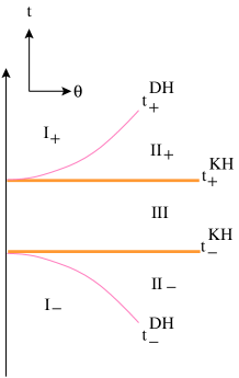
Figure 13: S-dihole II is actually several different solutions including regions I_±, II_± and III. Regions I_± and II_± are separated by null infinity at $t_{\pm}^{\rm DH}$ while region III is a signature $+---$ solution separated by a boundary at $t_{\pm}^{\rm KH}$.

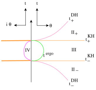
Figure 14: Applying a $\gamma$ flip to region III we find a $+++-$ S-brane solution where now $t_{\pm}^{\rm KH}$ are horizons. An ergosphere singularity lies in region III and $\theta=0$ is a horizon which leads to a new region IV. A complete picture of S-dihole II is in Fig. 18.

3.4.1 Piecing together the spacetimes

The six aforementioned regions are not the end of the spacetimes and their maximal extensions will include new regions III_± and IV_± (see Fig. 18). In total S-dihole II actually contains six different maximally extended universes, and so six card diagrams, which we describe here in Weyl language. Three of the spacetimes, which we label $\cal{E},\cal{E}_{\pm}$, are singular while $\cal{U},\cal{U}_{\pm}$ are non-singular. Further details in Weyl coordinates will also appear in Sec. 3.6.

The three ${\cal E}$ card diagrams are drawn in Figs. 16 and 16. Each diagram comprises 8 cards, 2 singular ergospheres, and is time symmetric. All of these card diagrams actually describes two universes, one on each side of the ergosphere. The ergosphere is located on the horizontal cards so the singularity is not naked from the point of view of any of the vertical cards.

The universe ${\cal E}$, comprising $t_{-}^{\rm DH}<t<t_{+}^{\rm DH}$, can be obtained by starting with the region III, $t_{-}^{\rm KH}\leq t\leq t_{+}^{\rm KH}$, and performing $\gamma\to\gamma+i\pi$. This universe is composed of two copies of regions II_±, III and IV. Region III is represented as a horizontal card with foci at $z=\pm\sqrt{M^{2}-a^{2}}$ and where the coordinate $t$ is conveniently parametrized as $t=M+\sqrt{M^{2}-a^{2}}\cos\zeta$. On this card the ergosphere is the curve $(M^{2}-a^{2})\sin^{2}\zeta=a^{2}\sinh^{2}\theta$ which ends on the two foci and extends outward to touch $(\rho,z)=((M^{2}-a^{2})/a,0)$. Along $z>\sqrt{M^{2}-a^{2}}$ region III attaches to region II₊ which is a $45^{\circ}$ wedge card $\rho^{\prime}<z-\sqrt{M^{2}-a^{2}}$. These wedges are bounded by special null lines $\rho^{\prime}=z-\sqrt{M^{2}-a^{2}}$ which are the Weyl coordinate representation of $t^{DH}$. We can further attach two more cards to form a four card junction; region III is connected to two II₊ cards, one pointing up and one pointing down, and another horizontal region III card in the back. Similarly along $z<-\sqrt{M^{2}-a^{2}}$ we have a four card junction, including two II_- cards. Surprisingly the line $-\sqrt{M^{2}-a^{2}}<z<\sqrt{M^{2}-a^{2}}$ is in fact also a horizon. Here we again have four cards including two copies of region IV which is a compact vertical wedge card $\rho^{\prime}<\sqrt{M^{2}-a^{2}}\pm z$. The card diagram is shown in Fig. 16. To understand this card diagram it is helpful to remember that the special null lines can represent conformal null infinity which is infinitely far away, and that the focal points themselves lie down throats and are infinitely far away. In Sec. 3.5.1 we explicitly demonstrate that the null lines here correspond to null infinity. As additional evidence one may check that the Riemann tensor squared vanishes along the null lines.

The universe ${\cal E}_{+}$ has $t>t_{+}^{\rm DH}$. This universe is composed of four copies of region I₊, and two copies of regions III₊ and IV₊. It is obtained by taking region I₊, which is a $45^{\circ}$ wedge noncompact vertical card in Weyl coordinates and turning it on its side via $\gamma\to\gamma+i\pi$. Instead of being a boundary, $\theta=0$ is now a horizon which we can go through to reach III₊. In Weyl coordinates this is one of the two horizons $|z|>\sqrt{M^{2}-a^{2}}$. Each horizon is a four card junction which attach to two copies of region I₊ and III₊ in the back. Region III₊ is qualitatively similar to region III and has foci at $z=\pm\sqrt{M^{2}-a^{2}}$ and an ergosphere along the line $(M^{2}-a^{2})\sinh^{2}\zeta=a^{2}\sin^{2}\theta$ running in the horizontal card. There is a further horizon $|z|<\sqrt{M^{2}-a^{2}}$ which attaches to a region IV₊ qualitatively similar to IV; it is a compact 45-45-90 wedge vertical card. In Weyl coordinates this region IV₊ can be found by starting with region IV and passing through the special null line $R_{-}=0$, where $R_{-}$ is the distance to the $t_{+}$ focus. The card diagram for this universe and the $\cal{E}_{-}$ universes, which we describe next, are shown in Fig. 16.

A third universe ${\cal E}_{-}$ has $t<t_{-}^{\rm DH}$. It is similar to ${\cal E}_{+}$ but it involves regions I_-, III_-, and IV_-. However since S-dihole II is not ‘time symmetric’ these are truly different universes. The ergosphere is specified by the same locus as for III₊. Region IV_- is Weyl-adjacent to IV and is gotten by passing the special null line $R_{+}=0$ where $R_{+}$ is the distance to the $t_{-}$ focus.

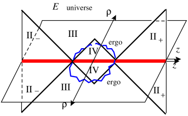
Figure 15: The $\cal{E}$ card diagram consists of eight cards and a singular ergosphere on the horizontal region III.

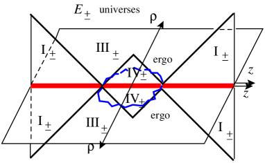
Figure 16: The $\cal{E}_{\pm}$ cards are similar to $\cal{E}$ and each other. The ${\cal E}_{-}$ universe has a ring singularity atop the ergosphere at $z=0$ (not pictured).

As for the three non-singular $\cal{U}$ universes, they consist of three vertical cards starting with one vertical $45^{\circ}$ wedge card joined at its tip to a compact $45$-$45$-$90$ card which is joined at its other tip to another vertical $45^{\circ}$ wedge card (see Fig. 17). The cards are joined pointwise at their tips by a de Sitter type near horizon scaling limit $\cal{W}$. Although the ${\cal U}$, ${\cal U}_{\pm}$ card diagram structures are time symmetric, the $\cal{U}$ universe itself is not time symmetric.

The universe ${\cal U}$ is composed of regions I_-, I₊, and IV. Take region I₊ which is the vertical wedge $0\leq\rho<\tau-\sqrt{M^{2}-a^{2}}$; in BL coordinates $t$ is time. At the corner of the wedge, we will see in Sec. 3.5.1 that the metric has a near-horizon scaling limit ${\cal W}$ which includes dS₂ in the coordinates $x^{4}$, and $\sigma$, where $\sigma$ loosely is the distance into the Weyl wedge from the corner. From our discussion of the third parabolic card representation for the Witten bubble, we know then that such a wedge card can connect to two regions ‘below the $t_{+}$ tip’ and they are precisely IV. Region I₊ is connected to region IV by crossing a horizon and performing an analytic continuation of $\theta$ and $\zeta$. Although this connection is unusual, if I₊ did not connect to any other region, the universe would have to begin at the tip of the wedge since $t$, or $\tau$ in Weyl coordinates, is a timelike variable. Similarly at the bottom region of IV, the $t_{-}$ tip attaches via ${\cal W}$ to two I_- wedges. This universe is not time symmetric. An interesting feature of these card diagrams is that we can see that region IV has both future and past null infinities, ${\cal I}^{\pm}$. They meet along the point at spacelike infinity. There is no easy Penrose diagram of the ${\cal U}$ universes. We must envision it as the card diagram with a dS₂ Penrose structure near each Weyl vertex.

The universe ${\cal U}_{+}$ is gotten from II₊, where $\theta$ is time. At the corner, we find ${\cal W}$ and this attaches to two copies of IV₊. At each other tip of IV₊, which is still at $t_{+}$, we attach two copies of II₊. This universe is time symmetric. Lastly ${\cal U}_{-}$ is gotten from II_- and IV_-. This universe is time symmetric.

It is important that the I_±, II_±, IV, IV_± wedges are free of ergosphere singularities, and that the ‘ring singularity’ $\Sigma=0$ occurs only as a point in III_-, and sits atop the ergosphere.

Figure 17: The $\cal{U}$ universes. Each pointlike intersection actually connects to two similar spacetimes as illustrated on the right.

As described earlier in Sec. 2.3.2 the Schwarzschild black hole, Witten bubble and S-Schwarzschild are all related by $\gamma$-flips and may be combined into one diagram. This diagram contains the information for all of their individual card diagrams. Similarly the combined multitude of S-dihole II regions is shown collectively in Fig. 18.

Figure 18: The regions of S-dihole II

3.4.2 Other ways to get the regions and analogy with Kerr

To complete our general description of the global structure of S-dihole II, we detail other ways to find the various regions in BL coordinates and the analogy between the (S-)dihole and (S-)Kerr geometries. To avoid confusion, we always use the name that applies in the Kerr geometry. For example even though the Kerr ergosphere is mapped by a Bonnor transformation to a singularity in S-dihole II, we still call it the ergosphere.

A simple way to obtain region III₊ is to begin with the $r\geq r_{+}$ portion of the dihole and analytically continue

$$t\to ix^{4},\hskip 21.68121pt\phi\to i\phi,\hskip 21.68121pta\to ia\ .$$ (28)

Region III_- can similarly be obtained from the $r\leq r_{-}$ portion of the dihole and continuing in the same way. If we start with a separated pair of one negative mass black hole and one positive mass one black hole instead of the dihole, we can similarly analytically continue and get region III. In Weyl coordinates this is achieved by sending $R_{-}\to-R_{-}$; in BL coordinates $\theta\to i\theta$ and $\zeta\to i\zeta$. We note that in the case of the Schwarzschild black hole, the analytic continuation in (28) and

$$t\to ix^{4},\hskip 21.68121pt\theta\to\pi/2+i\theta$$ (29)

both gave the Witten bubble just in different parametrizations. For the dihole, however, (28) does not give S-dihole I. This is clear since the analytic continuation in (28) leads to $\cal{E}_{+}$ universes which are singular, while S-dihole I is non-singular. The fact that these two analytic continuations give different spacetimes in the case of the dihole, is a result of its reduced $SO(2)$ rotational symmetry as compared to $SO(3)$ for Schwarzschild.

Regions III_± are Bonnor duals to horizontal cards in new S-Kerr universes ${\cal K}_{+}$ and ${\cal K}_{-}$ obtained by taking $t\to ix^{4}$, $\phi\to i\phi$, $a\to ia$ in Kerr and looking at $r\geq r_{+}$ and $r\leq r_{-}$ respectively. For these cases we must twist the $x^{4}$ and $\phi$ directions before compactifying $\tilde{x}^{4}$. These two spacetimes are different from the S-Kerr universe of [24] which in this notation can be called ${\cal K}$. All three ${\cal K}$ type universes have the same card diagram structure as elliptic (two Weyl foci) S-Schwarzschild. In the language of cards, the two nonidentical vertical quarter-plane cards of $\cal{K}$ can be turned on their sides and continued to yield ${\cal K}_{+}$ and ${\cal K}_{-}$.

For Kerr geometries, switching the roles of time and space Killing vectors means that the boundaries of the ergospheres and regions with closed timelike curves are interchanged. For Bonnor dual dihole geometries, the ergosphere $\Sigma-2Mr=0$ becomes a singularity and the CTC boundary does not map to anything immediately relevant.

The ‘ring singularity’ $\Sigma=0$ can persist as a singularity in some S-Kerr and dihole geometries. It may or may not overlap with the ergosphere singularity. For the dihole, there is no ergosphere for either $r\geq r_{+}$ or $r\leq r_{-}$, but there is a ring singularity which represents the actual black hole singularities, on the $r\leq r_{-}$ (both negative mass) horizontal card.

A magnetic dihole with magnetic potential $A_{\phi}$ becomes electrically charged after a double Killing rotation. Electric flux $*dA$ must then be computed with a metric, which is not well defined at say the ergosphere singularity. A dual magnetic potential $A_{4}$ is however well behaved at the singularity and the flux passes through the singularity on the card as if it were not there. For the black dihole, $A={2Ma\cos\theta dt/(r^{2}-a^{2}\cos^{2}\theta)}$ does blow up at the ring singularity, $\Sigma=r^{2}-a^{2}\cos^{2}\theta=0$.

3.5 Scaling limits

3.5.1 The $\theta$, $\zeta$ coordinates, ${\cal I}^{-}$, and the near-horizon limit

It is convenient to hyperbolically parametrize the region $t>t_{+}^{\rm KH}$ by $t=M+\sqrt{M^{2}-a^{2}}\cosh\zeta$. In this case the subextremal, $M>a$, S-dihole II solution is given by

$$ds^{2} = \Big{(}{\Sigma-2Mt\over\Sigma}\Big{)}^{2}\Big{(}(dx^{4})^{2}+{\Sigma^{4}(-d\zeta^{2}+d\theta^{2})\over(M^{2}-a^{2})^{3}(\sinh^{2}\zeta-\sinh^{2}\theta)^{3}}\Big{)}$$

$$+{(M^{2}-a^{2})\sinh^{2}\zeta\sinh^{2}\theta d\phi^{2}\over\big{(}{\Sigma-2Mt\over\Sigma}\big{)}^{2}},$$

$$A = {2aMt\sinh^{2}\theta\over\Sigma-2Mt}d\phi,$$

where $\Sigma-2Mt=(M^{2}-a^{2})\sinh^{2}\zeta+a^{2}\sinh^{2}\theta$ and $\Sigma=t^{2}+a^{2}\cosh^{2}\theta$. The locus $t_{+}^{\rm DH}$ is now simply $\theta=\zeta$ and $\zeta\geq\theta$ gives region I₊.

To see that the line $\theta=\zeta$ serves as ${\cal I}^{-}$, the relevant non-Killing part of the metric is

$${-d\zeta^{2}+d\theta^{2}\over(\sinh^{2}\zeta-\sinh^{2}\theta)^{3}}.$$

Let us change variables so $U={\zeta+\theta\over 2}$, $V={\zeta-\theta\over 2}$ where $U\geq V>0$. For small $V$ and staying away from small $U$, we have $ds^{2}\sim-dUdV/V^{3}$. Next define $v=-1/V^{2}$, $u=-1/U^{2}$, so the metric is $ds^{2}\sim-dudv$ for $v\leq u<0$. From these coordinate transformations it is clear that region $I_{+}$ extends infinitely far into the negative $v$ direction. The $uv$ chart has its own ${\cal I}^{+}$, $u=0$.

Next we examine the corner of the wedge where $\theta$ and $\zeta$ are small and find a near horizon dS₂ type scaling limit. Define $\theta=\sqrt{\sigma}\sinh\eta$, $\zeta=\sqrt{\sigma}\cosh\eta$ and scale the coordinates as $\sigma\to\sigma/\lambda$, $x^{4}\to\lambda x^{4}$, $\lambda\to\infty$. This gives the $\sigma>0$ half of a universe which we call ${\cal W}$

$$ds^{2} = ((M^{2}-a^{2})\cosh^{2}\eta+a^{2}\sinh^{2}\eta)^{2}\Big{(}{\sigma^{2}(dx^{4})^{2}\over\Sigma_{+}^{2}}+{\Sigma_{+}^{2}\over(M^{2}-a^{2})^{3}}(-d\sigma^{2}/4\sigma^{2}+d\eta^{2})\Big{)}$$

$$+{(M^{2}-a^{2})\Sigma_{+}^{2}\cosh^{2}\eta\sinh^{2}\eta d\phi^{2}\over((M^{2}-a^{2})\cosh^{2}\eta+a^{2}\sinh^{2}\eta)^{2}},$$

$$A = {2aMt_{+}^{\rm KH}d\phi\over a^{2}+(M^{2}-a^{2})\coth^{2}\eta}$$

where the constant $\Sigma_{+}=(t_{+}^{\rm KH})^{2}+a^{2}$. This universe is a fibering of dS₂ over the $\eta$ direction for $\eta\geq 0$. The magnetic field points along the $x^{4}$ direction and is finite and bounded. Although the ergosphere singularity apparently intersects the corner of the wedge, the singularity is smoothed out as we approach the corner by the shrinking of the space for small $\sigma$.

This is the first appearance of dS₂ as a nontrivial near-horizon limit in a non-spinning Einstein-Maxwell geometry. It might be interesting to search for a similar scaling limit in the extremal limit. We stress that this is not an E-brane solution.

3.5.2 Asymptotics: flat space

To better understand the S-dihole I and II, it is useful to study the spatial asymptotics. This can be done by taking a large-$\theta$ or large-$\zeta$ (or $r$ or $t$ in BL coordinates) scaling limit, whichever variable represents space. All large time limits give flat space with no conical singularity.

For the $r\geq r_{+}$ universe of S-dihole I, the large spatial limits are along the radial $r$ direction. Scaling the metric and coordinates $r\to\lambda r$, $x^{4}\to\lambda x^{4}$, $g_{\mu\nu}\to g_{\mu\nu}/\lambda^{2}$, and the vector potential $A\to A/\lambda$, we find that the vector potential scales to zero and we get the vacuum solution

$$ds^{2}=(dx^{4})^{2}+dr^{2}-r^{2}d\theta^{2}+r^{2}\cosh^{2}\theta d\phi^{2}.$$

The constraint $r\geq r_{+}$ scales to $r\geq 0$, and we have a Rindler wedge of flat space. Changing to Weyl coordinates, the metric is

$$ds^{2}=(dx^{4})^{2}+d\rho^{2}-d\tau^{2}+\rho^{2}d\phi^{2}\ .$$

Although this looks like flat space there is an asymptotic conical singularity as we earlier identified $\phi\simeq\phi+2\pi{a^{4}\over(M^{2}+a^{2})^{2}}$ to avoid a conical singularity near the origin. By an asymptotic conical singularity we mean that only asymptotically is the spacetime a cone. This solution is therefore interpreted as the creation of an S0-brane with energy per unit length equal to the deficit angle over $8\pi$, so $E/L={1\over 4}(1-(1+M^{2}/a^{2})^{-2})$ [35]. The $r\leq r_{-}$ S-dihole I universe gives the same result.

For S-dihole II superextremal, the $\theta$ coordinate is spacelike and we scale $e^{\theta}\to\lambda e^{\theta}$, $x^{4}\to\lambda x^{4}$, $g_{\mu\nu}\to g_{\mu\nu}/\lambda^{2}$, $A\to A/\lambda$. In this limit the solution again simplifies to a vacuum solution

$$ds^{2}=(dx^{4})^{2}+{a^{8}\over(a^{2}-M^{2})^{3}}(-R^{2}d\zeta^{2}+dR^{2})+(a^{2}-M^{2})R^{2}\cosh^{2}\zeta d\phi^{2},$$ (30)

where $t-M=\sqrt{a^{2}-M^{2}}\sinh\zeta$ and $-\infty<\zeta<\infty$ parametrizes a Rindler wedge. Changing to dimensionless Weyl coordinates, the metric becomes

$$ds^{2}=(dx^{4})^{2}+{a^{8}\over(a^{2}-M^{2})^{3}}(-d\tau^{2}+d\rho^{2})+(a^{2}-M^{2})\rho^{2}d\phi^{2}.$$ (31)

The angular $\phi$ was previously periodically identified with $\phi\simeq\phi+2\pi$ to avoid a conical singularity at the origin so S-dihole II has an asymptotic conical singularity. We have created an S0-brane with $E/L={1\over 4}(1-(1-M^{2}/a^{2})^{2})$.

Next let us examine the large-$\theta$ limit of the S-dihole II subextremal solutions. If we attempt to take the large-$\theta$ limit for S-dihole II subextremal in region I₊ of the ${\cal U}$ universe, we move into region II₊. So large spatial limits cannot be taken in the same way here. However if we $\gamma$-flip region I₊ so it is part of the ${\cal E}_{+}$ universe, then a large spatial limit gives the Milne wedge. The large spatial limits of the horizontal cards III, III_± are also just Rindler wedges; there are no conical singularities, or Rindler or Milne orbifolds.

Finally the compact wedges IV, IV_± interpolate from one ${\cal W}$ to the same or another one, either $\Sigma_{-}\to\Sigma_{+}$, $\Sigma_{+}\to\Sigma_{+}$, or $\Sigma_{-}\to\Sigma_{-}$. If we regard them as part of the ${\cal U}$ universes, then IV_± are time-symmetric, while IV is not. While these regions have ${\cal W}$ as timelike scaling limits, it is not clear if they have spacelike scaling limits.

3.5.3 Melvin scaling and KK CTCs

While the above two scaling limits are new, there is also a known scaling limit of the dihole [36] and S-dihole I [19] which gives the Melvin universe [12, 13]. The Melvin universe has an axially symmetric magnetic field which decays to zero in the transverse direction. The quantity $\Sigma-2Mr$, whose zero locus yields the ergosphere singularity, is the quantity of interest yielding the nontrivial spatial dependence; both the parameters $M$, $a$, and $\tilde{\theta}=\theta-\pi/2$, $\zeta$ must be scaled such that $\tilde{\theta}\sim\zeta\to 0$ and $M\zeta\sim a$. In this limit we have $M\gg a$.

The dihole and S-dihole I are related by analytic continuation, and the Melvin universes which come from the dihole and S-dihole I are actually from the same neighborhood of their complexified 4-manifolds. Since the $r\geq r_{+}$ dihole can be continued to region III₊, and IV₊ is directly adjacent near $\rho=0$, $z=0$, we must also have a Melvin scaling limit in IV₊. For $r\leq r_{-}$, similar remarks apply to III_- and IV_-. As part of the ${\cal U}_{\pm}$ universes, IV_± scale to

$$ds^{2} = \Big{(}{a^{2}+\rho^{2}\over 4M^{2}}\Big{)}^{2}\Big{(}{4M^{2}\over a^{2}}\Big{)}^{4}\big{(}(dx^{4})^{2}-d\tau^{2}+d\rho^{2}\big{)}+\big{(}{4M^{2}\over a^{2}+\rho^{2}}\big{)}^{2}\rho^{2}d\phi^{2}$$ (32)

$$A = -a\tau dx^{4}/2M^{2}.$$

As part of the ${\cal E}_{\pm}$ universes, we must turn (32) on its side to yield a 4-card S-Melvin scaling limit, with an ergosphere singularity on the horizontal cards.

There is no corresponding Melvin scaling limit for regions III, IV, or for the superextremal S-dihole II.

The ergosphere singularity of a dilatonized version of S-Melvin was found and discussed in [22]. Just as dilatonized Melvin can be obtained by twisting a completely flat KK direction with an azimuthal angle, S-Melvin can be obtained by twisting a completely flat KK direction with a boost parameter. The ergosphere singularity is then where the twisted KK direction becomes null. On one side of the ergosphere singularity (small $\rho$ on the horizontal card), the twisted KK direction is spacelike whereas on the other side (large $\rho$ on the horizontal card) it is timelike yielding a KK CTC.

Actually, this is a general feature of ergosphere singularities. One may wonder about the following connection: The ‘ergosphere,’ where a timelike Killing direction of say Kerr becomes null and switches to spacelike, maps via the Bonnor transformation to an ergosphere singularity of say the ${\cal E}$ S-dihole II, where a dilatonized version has a KK circle changing signature. The precise connection is that the Bonnor transformation can be understood from the KK perspective in reducing from five to four dimensions. If we take a dihole-type solution (19) and dilatonize it with $\alpha=\sqrt{3}$ [7] we get

$$ds_{\rm dil}^{2} = -f^{1/2}dt^{2}+f^{-1/2}\big{(}e^{2\gamma}(d\rho^{2}+dz^{2})+\rho^{2}d\phi^{2}\big{)}$$

$$A_{\rm dil} = {1\over 2}Bd\phi$$

$$e^{2\phi} = f^{\sqrt{3}/2}.$$

Lifting to 5 dimensions [32][19], we get

$$ds_{\rm 5d}^{2}=f(dx^{5}+Bd\phi)^{2}-dt^{2}+f^{-1}\big{(}e^{2\gamma}(d\rho^{2}+dz^{2})+\rho^{2}d\phi^{2}\big{)},$$

and the Killing $t_{\rm dihole}$ becomes completely flat. It may be dropped and the resulting 4d solution is a Kerr-type instanton. Upon Wick rotating $x^{5}\to it_{\rm Kerr}$ and $B\to-i\omega$, the $x^{5}$ direction becomes Kerr time. Hence $x^{5}$ and $t_{\rm Kerr}$ change signature on the same complexified locus, the ‘ergosphere.’

3.6 Weyl Coordinates

Here we give the Weyl description of S-dihole II and discuss some technical details involving branches.

In Weyl coordinates for the dihole

$$\rho=\sqrt{r^{2}-2Mr-a^{2}}\sin\theta,\qquad z=(r-M)\cos\theta$$

the Wick rotation (24) is the same as

$$t\rightarrow ix^{4},\hskip 21.68121ptz\rightarrow i\tau,\hskip 21.68121ptM\to iM.$$ (33)

This means that S-dihole II can be easily obtained by sending $M\to iM$ in S-dihole I of [19]. This also makes it clear that the foci for S-dihole II are at $z=\pm\sqrt{M^{2}+a^{2}}\to\tau=\pm\sqrt{M^{2}-a^{2}}$ in Weyl space and therefore we get the special null lines for $|M|>|a|$ and not for $|M|<|a|$.

Due to the square roots which appear in Weyl functions, however, there is a branch choice to make for $R_{\pm}$ and this will sometimes generate an additional choices for signs in the solution. Previously we have noted that $R_{\pm}$ will change sign across a special null line and in fact this is precisely what will account for the branch choices in subextremal S-dihole II.

The magnetic dihole in Weyl coordinates is $ds^{2}=-fdt^{2}+f^{-1}(e^{2\gamma}(d\rho^{2}+dz^{2})+\rho^{2}d\phi^{2})$ with

$$f = \left[{(R_{+}+R_{-})^{2}-4M^{2}-{a^{2}\over M^{2}+a^{2}}(R_{+}-R_{-})^{2}\over(R_{+}+R_{-}+2M)^{2}-{a^{2}\over M^{2}+a^{2}}(R_{+}-R_{-})^{2}}\right]^{2}$$ (34)

$$e^{2\gamma} = \left[{(R_{+}+R_{-})^{2}-4M^{2}-{a^{2}\over M^{2}+a^{2}}(R_{+}-R_{-})^{2}\over 4R_{+}R_{-}}\right]^{4}$$

$$A = {aM(R_{+}+R_{-}+2M)(1-{(R_{+}-R_{-})^{2}\over 4(M^{2}+a^{2})})\over{1\over 4}(R_{+}+R_{-})^{2}-M^{2}-a^{2}{(R_{+}-R_{-})^{2}\over 4(M^{2}+a^{2})})}d\phi,$$

$$R_{\pm} = \sqrt{\rho^{2}+(z\pm\sqrt{M^{2}+a^{2}})^{2}}.$$ (35)

Analytically continuing $t\to ix^{4}$, $z\to i\tau$ and $M\to iM$, gives S-dihole II. However, in the superextremal case, the quantity $R_{+}+R_{-}+2M$ appearing in $f$ is no longer real, since $R_{\pm}$ are complex conjugates. The problem is that a transformation equation like $2(r-M)=R_{+}+R_{-}$ no longer makes sense when doing the analytic continuations in both coordinate systems. The problem is remedied by replacing all instances of $R_{-}$ by $-R_{-}$ in (34); this is a choice of branch. This sign change is common in Weyl solutions; if we replace $R_{-}\to-R_{-}$ in (34), we get the solution for the interior of the black hole at $R_{-}=0$ (and also the universe where we have a negative mass object ‘centered’ at $R_{-}=0$ and an extremal black hole at $R_{+}=0$). In particular changing this sign maintains the status of these functions as solutions to the Einstein-Maxwell system.

To demonstrate the necessity of changing $R_{-}\to-R_{-}$ in the superextremal case, we begin by simplifying the transformation formulas for the dihole by introducing the coordinate $\zeta$ through the relation $r-M=\sqrt{a^{2}+M^{2}}\cosh\zeta$ so in this new variable we have $\rho=\sqrt{a^{2}+M^{2}}\sinh\zeta\sin\theta$, $z=\sqrt{a^{2}+M^{2}}\cosh\zeta\cos\theta$ and $R_{\pm}=\sqrt{a^{2}+M^{2}}(\cosh\zeta\pm\cos\theta)$. Now perform the analytic continuation of (24). To effect the analytic continuation $r\to it$ we must shift $\zeta\to\zeta+i\pi/2$, so $\cosh\zeta\to i\sinh\zeta$. In this case we get $t-M=\sqrt{a^{2}-M^{2}}\sinh\zeta$ and $R_{\pm}=\sqrt{a^{2}-M^{2}}(i\sinh\zeta\pm\cosh\theta)$. The sum $R_{+}+R_{-}$ is purely imaginary, as required to ensure that the metric in (34) is real.

For the subextremal case, we do not shift $\zeta$. The solution is real, with any branch choice, to the left of both special null lines on the vertical card. With

$$\rho=\sqrt{t^{2}-2Mt+a^{2}}\sinh\theta,\qquad\tau=(t-M)\cosh\theta$$

the $t>t^{\rm KH}_{+}$ region can be covered by $t-M=\cosh\zeta\sqrt{M^{2}-a^{2}}$ as

$$\rho=\sqrt{M^{2}-a^{2}}\sinh\zeta\sinh\theta,\qquad\tau=\sqrt{M^{2}-a^{2}}\cosh\zeta\cosh\theta.$$

Since $\sinh\zeta\sinh\theta+1\leq\cosh\zeta\cosh\theta$, we see this covers $\tau\geq\rho+\sqrt{M^{2}-a^{2}}$ twice. Both $\theta=0$ ($\zeta>0$) and $\zeta=0$ ($\theta>0$) lie on the $\tau\geq\sqrt{M^{2}-a^{2}}$ semiaxis; this is where the $\phi$-circle vanishes in a smooth or conical singularity fashion. The envelopes of $\theta$- or $\zeta$-orbits are the line $\tau=\rho+\sqrt{M^{2}-a^{2}}$, which is precisely $t=t^{\rm DH}_{+}$ and is a coordinate singularity in BL or Weyl coordinates. This is a special null line separating region I₊ from I_- and we have previously demonstrated that it serves as ${\cal I}^{-}$.

Since $R_{\pm}=i\sqrt{M^{2}-a^{2}}(\cosh\zeta\pm\cosh\theta)$, we see that interchanging $\theta\leftrightarrow\zeta$ sends $R_{-}\to-R_{-}$ in (34). If we take the convention that $R_{\pm}=\pm i\tau+i\sqrt{M^{2}-a^{2}}$ at $\rho=0$, then the large-$t$ wedge involves $R_{+}-R_{-}+2iM$ and the large-$\theta$ wedge involves $R_{+}+R_{-}+2iM$. The former branch (regions I_±) can be identified with the superextremal S-dihole II upon making $M^{2}-a^{2}$ negative, again explaining the superextremal solution’s branch.

So far we have built the vertical card for the subextremal S-dihole II. To obtain the region $t^{\rm KH}_{-}<t<t^{\rm KH}_{+}$ in the $\cal{E}$ universes we analytically continue $\rho\to i\rho^{\prime}$ and use

$$\rho^{\prime}=\sqrt{M^{2}-a^{2}-(t-M)^{2}}\sinh\theta,\qquad\tau=(t-M)\cosh\theta.$$

Changing to prolate angle $0\leq\eta\leq\pi$, we get

$$\rho^{\prime}=\sqrt{M^{2}-a^{2}}\sin\eta\sinh\theta,\qquad\tau=\sqrt{M^{2}-a^{2}}\cos\eta\cosh\theta.$$

This is then the usual horizontal spacelike Weyl half-plane, except there is an ergosphere singularity. The ergosphere is a line segment which is symmetric in the coordinate $\tau\to-\tau$, and touches the points $(\rho^{\prime},\tau)=(0,\pm\sqrt{M^{2}-a^{2}})$ on the horizon and $(\rho^{\prime},\tau)=((M^{2}-a^{2})/a,0)$ in the interior of the card. The $\phi$ direction is timelike on the horizontal card and has horizons along $\rho^{\prime}=0$, $\tau>\sqrt{M^{2}-a^{2}}$ or $\tau<-\sqrt{M^{2}-a^{2}}$ with Euclidean periodicity (27), and another horizon inside the ergosphere singularity with Euclidean periodicity $2\pi$ for $-\sqrt{M^{2}-a^{2}}<z<\sqrt{M^{2}-a^{2}}$. For the region inside the ergosphere we can continue to two vertical cards IV at non-primed $\rho$, much like the Schwarzschild card diagram. However in this case the spacetimes ends at the special null lines which serve as ${\cal I}^{\pm}$.

The Weyl foci are an infinite distance from the interior of the III card from either inside or outside the ergosphere.

Finally we discuss how the three regions of each ${\cal U}$ universes are pieced together on the same Weyl vertical $\rho$, $\tau$ card (see Figure 17). Label the three pieces $W_{1}$, $W_{2}$, and $W_{3}$ in chronological order so as time passes we proceed from $W_{1}$ to $W_{2}$ to $W_{3}$. These three wedges are bounded by two lines $0\leq\rho\leq|\tau\pm\sqrt{M^{2}-a^{2}}|$. The key point is that these are null lines so when we cross from one wedge to another, we must change branches of the Weyl functions $R_{\pm}$. Label the null lines so $S_{1}$ refers to the special null lines from $\tau=-\sqrt{M^{2}-a^{2}}$ and $S_{2}$ refers to the special null lines from $\tau=\sqrt{M^{2}-a^{2}}$. Label the two different branches for $S_{1}$ as $\pm$ and similarly for $S_{2}$. A spacetime region is then specified by the four possible branches relative to the two null lines. Region $W_{1}$ can then be labelled by the branches $(-,-)$, while $W_{2}$ is then $(+,-)$ since we have passed $S_{1}$, and $W_{3}$ is $(+,+)$ since we have also passed $S_{2}$. These three regions are pieced together to give ${\cal U}$, with its wedges I_-, IV, and I₊. Similarly, the ${\cal U}_{+}$ has three wedges labelled by $(-,+)$, $(+,+)$, $(+,-)$, and the three wedges of ${\cal U}_{-}$ are $(+,-)$, $(-,-)$ and $(-,+)$.

3.7 S-Charge

For an S-brane solution with electric field, the magnetic S-charge [3]-[37] is defined as the integral of $F$ over a two dimensional surface ${\cal S}$ which is spacelike and transverse to the brane direction. In the absence of sources or singularities and with sufficient decay of fields at infinity, the S-charge is conserved in the sense that it does not depend on ${\cal S}$.

In [19] the S-charge of S-dihole I for $r\geq r_{+}$ was computed in Weyl coordinates over a constant-$\tau$ slice to be $Q_{s}={M\over a}(M+\sqrt{M^{2}+a^{2}})$ and was shown to be conserved. The S-charge along a constant-$t$ slice in BL coordinates can be shown to give the same result. The region $r\leq r_{-}$ S-dihole I has a constant S-charge which has a value equal to putting $M\to-M$ in the above formula.

The S-dihole II (26) has a vector potential

$$A={2aMt\sinh^{2}\theta\over t^{2}-2Mt+a^{2}\cosh^{2}\theta}d\phi.$$

The superextremal $|a|>|M|$ spacetime is globally simple in that it is free of horizons, singularities and special null lines. To compute the S-charge on a BL slice, we fix $t$ and integrate $F_{\theta\phi}$

$$Q_{s}={1\over 4\pi}\int_{0}^{2\pi}d\phi\int_{0}^{\infty}d\theta{\partial\over\partial\theta}\Big{(}{2aMt\sinh^{2}\theta\over t^{2}-2Mt+a^{2}\cosh^{2}\theta}\Big{)}=Mt/a.$$

This is not conserved, and is due to the fact that $F_{t\phi}$ does not decay fast enough; as $\theta\to\infty$ the $dtd\phi$ flux integral is

$$d\Phi_{\infty}={4\pi M\over a}dt.$$

Trying to get this result directly from our knowledge of S-dihole I, whose S-charge is $Q_{s}={M\over a}(M+\sqrt{M^{2}+a^{2}})={M\over a}(M+{R_{+}+R_{-}\over 2})$ evaluated at $r=r_{+}$. This Wick rotates in our prescription to $Q_{s}=-{M\over a}(M+{R_{+}-R_{-}\over 2i})=-Mt/a$ which is right (up to an overall sign which we do not keep track of).

On the other hand, it is possible to fix the time coordinate $\tau$ in Weyl coordinates for this superextremal S-dihole II and calculate the S-charge. In this case $A|_{\rho=0}=0$ and $A|_{\rho\to\infty}=-2M^{2}/a$ so the S-charge is $Q_{s}=M^{2}/a$. This result is independent of $\tau$ and so the S-dihole II has a ‘conserved’ charged in a limited sense.

Compared to the S-charge in BL coordinates, the S-charges are the same for $t=M$ (or $\tau=0$) which is where the solution experiences a ‘bounce.’ The difference between the BL and Weyl S-charges can be seen from looking at the surfaces ${\cal S}$ in Weyl coordinates: The BL constant-$t$ slice asymptotes to a finite, nonzero slope at large values of $\theta$ as shown in Fig. 19.

Figure 19: Calculation of S-charge on Boyer-Lindquist versus Weyl time slices can lead to different results.

Examining the EM field strength for S-dihole II in the ${\cal E}$ universe, we notice the following fact. On the horizontal III card there is an electric field in the $t$ direction and for large values of $\theta$ $F_{\phi t}=2M/a$ is constant. One can then interpret this as an background electric field which is related to the two dimensional object along the ergosphere. As time passes (we eventually go up the vertical II_± cards) the electric field eventually goes to zero so this gives support for the interpretation of this S-dihole II as the creation of a localized two dimensional unstable object. The vertical II_± cards are entirely accessible to timelike observers who start on the horizontal III card, and yet they have spacelike Killing directions which yield spacetime points not accessible to any one observer. In contrast S-dihole I is the formation and decay of a localized fluxbrane, which would be a one dimensional object. The S-charge is finite and roughly corresponds to the fluxbrane charge which is conserved. The main electro-gravitational wave activity of S-dihole I is concentrated along the light cone.

The subextremal case is less amenable to S-charge. The noncompact wedge universes which are regions I_± and II_± have finite and nonconstant S-charge as we compute along a constant-time (say BL time $t$) slice out to the boundary. However, these surfaces ${\cal S}_{t}$ asymptote to the conformal infinity ${\cal I}^{\pm}$, not to $i^{0}$. Any attempt to find a surfaces to $i^{0}$ gives an infinite S-charge.

On the other hand, the compact wedge universes have a clear $i^{0}$ on the card diagram. S-charges are conserved and finite; one evaluates $A_{\phi}$ at $i^{0}$ and subtracts $A_{\phi}$ evaluated anywhere on the $\rho=0$ boundary. The S-charges are $Q_{s}^{-}={M\over a}(M-\sqrt{M^{2}-a^{2}})$, $Q_{s}=a$, and $Q_{s}^{+}={M\over a}(M+\sqrt{M^{2}-a^{2}})$ for regions IV_-, IV, and IV₊. Evidently, one can define an S-charge in the middle of the ${\cal U}$ universes (between the horizons) but not in the future or past regions. The results for $Q_{s}^{+}$ and $Q_{s}^{-}$ match the S-charge for the $r\geq r_{+}$ and $r\leq r_{-}$ S-dihole I, where we naively continue $M\to iM$.

4 Infinite alternating array

In the previous section we discussed some of the simplest S-brane solutions sourced by black holes. In this section we find black hole and S-brane solutions that generalize the infinite alternating array of [19]. The motivation for studying such arrays arises from the rolling tachyon solution [23] which was obtained by Wick rotating a periodic array of codimension one branes and anti-branes. These array solutions should also exist for any codimension, however, including the codimension three case which are Israel-Khan arrays black holes in four dimensions. Analytic continuation then produces S0-brane solutions in four dimensions or this configuration may be lifted to S6-branes in ten dimensions.

More specifically the array solutions were Israel-Khan arrays of black holes and in Weyl coordinates they are rods of length $2M$ whose midpoints are separated by a distance $2k$. When $\alpha=M/k<1$, the black holes rods do not overlap and upon twisted KK reduction, give alternating-charge extremal black holes. The conical singularities between the rods and on the rods can be removed by appropriately choosing constants $\gamma_{\rm divergent}$ and $U_{\rm divergent}$, while a dimensionful constant $R$ can be fixed to scale the black hole charges.

The solution with dilaton has a vector potential $A={\rho^{2}R\over 2(\rho^{2}+R^{2}e^{4U})}d\phi$. When $\alpha<1/2$ the rods occupy less than half of the $z$-axis, and we will take a symmetric setup where no rods cross $z=0$. In the limit $\rho\to\infty$, we have $U\sim\alpha\log\rho+{\rm consant}$, so $A\to Rd\phi/2$ and the S-charge (or rightwards flux through $z=0$) is $R/4$. The black hole charge is still $R/4$ as in [19], so that means that the rightwards flux through $z=-k$ vanishes. We see that the symmetrical set-up of $\alpha=1/2$ in [19] where S-charge flux alternates from pointing right to left with magnitude $R/8$, upon slightest deformation to $\alpha<1/2$, changes discontinuously so S-charge vanishes between close neighbor pairs and is all lumped between far neighbor pairs.

The case $\alpha>1/2$ yields a spacetime physically equivalent to a spacetime with parameter $1-\alpha$. In particular the S-charge never points the ‘wrong way’ as it does in the $a<0$ ‘anomalous’ region of the dihole-in-Melvin of [21]. The solutions we have are analogous to the $a=0$ case of dihole-in-Melvin.

We can continue $z\to i\tau$ to get a generalized alternating S-brane solution with a doubled S-charge $R/4$. Alternatively if a rod had crossed $z=0$ we would get a solution with S-charge $0$. We write the solution as

$$ds^{2} = (e^{2U}+e^{-2U}\rho^{2}/R^{2})^{1/2}((dx^{4})^{2}+e^{-2U}e^{2\gamma}(d\rho^{2}-d\tau^{2}))+\frac{\rho^{2}}{e^{2U}+e^{-2U}\rho^{2}/R^{2}}d\phi^{2}$$

$$A = \frac{\rho^{2}R}{2\rho^{2}+2R^{2}e^{4U}}d\phi$$

$$e^{-4\Phi/\sqrt{3}} = e^{2U}+e^{-2U}\rho^{2}/R^{2}$$

$$e^{2U} = e^{-2U_{\rm div}}\prod_{p=-\infty}^{\infty}\frac{r_{p}+\tilde{r}_{p}-2M_{p}}{r_{p}+\tilde{r}_{p}+2M_{p}}$$

$$e^{2\gamma} = e^{-2\gamma_{\rm div}}\prod_{p,q=-\infty}^{\infty}\frac{\tilde{r}_{q}r_{p}-(\tau+iz_{q}+iM_{q})(\tau+iz_{p}-iM_{p})+\rho^{2}}{\tilde{r}_{q}\tilde{r}_{p}-(\tau+iz_{q}+iM_{q})(\tau+iz_{p}+iM_{p})+\rho^{2}}\ \times$$

$$\frac{r_{q}\tilde{r}_{p}-(\tau+iz_{q}-iM_{q})(\tau+iz_{p}+iM_{p})+\rho^{2}}{r_{q}r_{p}-(\tau+iz_{q}-iM_{q})(\tau+iz_{p}-iM_{p})+\rho^{2}}$$

$$r_{p} = \sqrt{\rho^{2}-(\tau+iz_{p}+iM_{p})^{2}},\hskip 14.45377pt\tilde{r}_{p}=\sqrt{\rho^{2}-(\tau+iz_{p}-iM_{p})^{2}}$$ (36)

where $z_{p}=(2p+1)k$, $M_{p}=M$, tilde means to the left end of the rod [5], and there is no problem taking the standard branch cut for square roots. Using $r_{p}^{*}=-\tilde{r}_{-p-1}$, it is easy to see that $U$ is real, where every rod matches up with its image under ${\rm Im}\,\tau\to-{\rm Im}\,\tau$. The reality of $\gamma$ follows from its PDE.

As described in [38], we can deform the black hole locations while keeping the real-$\tau$ geometry real, as long as they obey the symmetry of charge conjugation times ${\rm Im}\,\tau\to-{\rm Im}\,\tau$. This means we may perform some further operations to deform our S-brane geometry. For example we may change the individual masses $M_{p}\to\lambda_{p}M_{p}$ as long as $\lambda_{p}^{*}=\lambda_{-p-1}$. We may also move the positions $z_{p}$ in the complex $z$-plane as long as ${\rm Re}\,z_{p}=-{\rm Re}\,z_{-p-1}$. Although naively the rules prohibit black holes from being on the real $\tau$-axis, in fact one or more rods may cross the real $\tau$-axis. Under these deformations, the original $z$-geometry is not real, or if it were, it has conical singularities; the $\tau$-geometry is however real and smooth. Note that non-finite deformations can require an infinite shift in $U_{\rm div}$, $\gamma_{\rm div}$.

From the S-dihole II geometry we known that we can place black holes on the real $\tau$-axis. This breaks the rule of [38] but seemingly restricts us to wedge universes instead of a full vertical card. Take for the present scenario a rod setup where there is a central rod $p=0$ that crosses $z=0$. This rod has no pair, and the only option for rotation is by $90^{\circ}$, $M_{0}\to iM_{0}$. The function $f_{0}={r_{0}+\tilde{r}_{0}+2iM\over r_{0}+\tilde{r}_{0}-2iM}$ is now real but only in the Weyl regions $\rho\leq|\tau\pm M|$. This comprises two noncompact wedge cards and one compact 45-45-90 wedge card. Let us call the Weyl wedges $W_{1}$, $W_{2}$, $W_{3}$ in chronological order. The solution is different from S-dihole II in Melvin in that there are the other rods at complex time $\tau$, which we anticipate smoothly deform the solution.

As discussed in Sec. 5.3.1, there are actually different branch choices for the pairs of rods at complex $\tau$. We will not focus on this because any good branch choice for these complex sources will be constant over the connected spacetime.

The rule for branches for $p=0$ is as follows. We may pick any set of branches in wedge $W_{1}$. Then when we pass through the dS₂ horizon to wedge $W_{2}$, we must change the branch for $\tilde{r}_{0}$. Now we are in wedge $W_{2}$. When we pass through the dS₂ horizon to wedge $W_{3}$, we must change the branch for $r_{0}$. This gives three distinct non-singular ${\cal U}$ type universes, where the branch choices are $(-,-)$, $(+,-)$, $(+,+)$ which is like ${\cal U}$ (or its time-reverse); $(+,-)$, $(-,-)$, $(-,+)$ which is like ${\cal U}_{-}$, and $(-,+)$, $(+,+)$, $(+,-)$ which is like ${\cal U}_{+}$.

One could take any of these wedges with a branch choice and turn the wedge on its side, yielding an ${\cal E}$ universe. Looking at the pure Einstein-Maxwell solution,

$$ds^{2} = (e^{2U}+e^{-2U}\rho^{2}/R^{2})^{2}((dx^{4})^{2}+e^{-8U}e^{8\gamma}(-d\tau^{2}+d\rho^{2})+(e^{2U}+e^{-2U}\rho^{2}/R^{2})^{-2}\rho^{2}d\phi^{2}$$

$$A = {\rho^{2}R\over\rho^{2}+R^{2}e^{4U}}d\phi,$$

we note that putting $\rho\to i\rho^{\prime}$ gives us possible zeroes for $e^{2U}-e^{-2U}\rho^{\prime 2}/R^{2}$. Comparing to the form of S-dihole II, this is precisely an ergosphere singularity. Its locus may be hard to describe but we expect for this single rod that the locus is qualitatively similar to that of S-dihole II. This solution is constituted in the same manner as the rolling tachyon[23] in that they are Wick rotations of an infinite array of branes and anti-branes.

One can put more than one vertical rod on the real $\tau$-axis. To put an even number, start with rods none of which cross $z=0$, and move an even number to real $\tau$. To put an odd number, start with rods one of which crosses $z=0$. In any case, the geometry will be real for $\rho\leq|\tau-\tau_{i}|$ for all foci $\tau_{i}$. If we put $n$ rods, then we have an initial noncompact wedge followed by $2n-1$ compact wedges and then one final noncompact wedge. We may pick any choice for initial branches, and as we pass through each dS₂ horizon at all the $\tau_{i}$, we change the branch of $R_{i}$.

If the divergent constant renormalization procedure does not break down, then it is possible to put an infinite number of rods along the real $\tau$-axis. Then we can have a universe which is periodic in time and has an infinite number of dS₂ horizons. To get periodicity in time, the only acceptable scheme of branches is to go, across a given focus, from $(\cdots,-,-,+,+,+,\cdots)$ to $(\cdots,-,-,-,+,+,\cdots)$, which is the same.

5 Card diagrams

In this section we construct the card diagrams for a wide assortment of solutions including black holes and S-branes. The card diagrams are shown to be useful in representing global spacetime structure such as how Reissner-Nordstrøm black holes change as we take their chargeless and extremal limits. For the superextremal black holes we discuss for the first time the technical issue of how to deal with the appearance of branch points in Weyl coordinates. The card diagram also clearly represents the Kerr ring singularity and how it is possible to traverse the ring into a second asymptotic spacetime. In addition the five dimensional black ring solution, which is a black hole with non-spherical horizon topology, is analyzed. Many other examples are presented.

5.1 Black holes

5.1.1 Reissner-Nordstrøm

In Weyl coordinates the Reissner-Nordstrøm black hole is

$$\rho = \sqrt{r^{2}-2Mr+Q^{2}}\sin\theta,\hskip 21.68121ptz=(r-M)\cos\theta$$ (37)

$$R_{\pm} = \sqrt{\rho^{2}+(z\pm\sqrt{M^{2}-Q^{2}})^{2}}=r-M\pm\sqrt{M^{2}-Q^{2}}\cos\theta$$

$$f = \frac{(R_{+}+R_{-})^{2}-4(M^{2}-Q^{2})}{(R_{+}+R_{-}+2M)^{2}}$$

$$e^{2\gamma} = \frac{(R_{+}+R_{-})^{2}-4(M^{2}-Q^{2})}{4R_{+}R_{-}}$$

$$A = -\frac{2Qdt}{R_{+}+R_{-}+2M}$$

and the card diagram for $|Q|<|M|$ is shown in Fig. 21. The construction of the card diagram proceeds along similar lines to the Schwarzschild card diagram. There are two adjacent horizontal half-planes, H1 and H2, which represent the positive mass asymptotically flat regions. The outer horizon is a rod which lies on the $z$-axis for $-\sqrt{M^{2}-Q^{2}}<z<\sqrt{M^{2}-Q^{2}}$. The vertical cards, V1 and V2, are squares of length $2\sqrt{M^{2}-Q^{2}}$ and the diagonal lines connecting opposite corners of the square are special null lines. In the Schwarzschild case, the black hole singularity is at the top of the vertical card V1 and the bottom of the card V2. When the black hole is charged, however, these vertical cards end in horizons with four card junctions. (In going past the two special null lines, the orientation of the $z$-axis has flipped direction.)

The vertical card ends at the inner horizon and connects to another vertical card as well as two horizontal half plane cards each containing a region h1 and h2 where $0<r<r_{-}$, and also a negative-mass universe. The black hole singularity lies on the boundary of the h1 and h2 regions and takes the form of a semi-ellipse $\rho^{2}/Q^{2}+z^{2}/M^{2}=1$. The black hole singularity is typically where we stop the space. For completeness though we extend past the singularity on the card diagram. For the case of charged black holes, negative values of $r$ lead to a nakedly singular spacetime. In fact this singular spacetime is exactly what fills out the rest of the horizontal card with the regions h3 and h4. The card diagram correctly captures the fact that negative mass universes do not have horizons and that their singularity is timelike.

Finally at each horizon, the card diagram should be continued vertically through horizons to obtain a tower of cards extending infinitely up and down in the vertical direction.

Let us compare this Weyl card diagram to the Reissner-Nordstrøm Penrose diagram. The Penrose diagram for all black holes with $M>|Q|$ are the same (see Figure 21), so the causal structure is the same for all such black holes. When $Q=0$ however spacetime is described by the Schwarzschild Penrose diagram of Fig. 1 which is very different. At once this tells us both that there is a discontinuous jump in the causal structure, but also that this discontinuity is not easy to understand from the Penrose diagram.

On the other hand the limit $Q\to 0$ is easy to understand by examining the Weyl card diagram in Figure 21. In this case the vertical cards expands to a $2M\times 2M$ square and the singularity, which formed a semi-ellipse, degenerates to a line segment covering the inner horizon. This singularity now sits on and seals the horizons and the multiple asymptotic regions from each other. So while in the presence of charge the singularity used to be timelike and avoidable, it now becomes spacelike as seen from the vertical card $0<r<2M$. Therefore a nice feature of the card diagram is that it shows how regions h1, h2 collapse and the singularity smoothly falls onto the vertical cards V1 and V2. An explorer on the vertical card who could continue up forever in the case of a charged black hole, is now doomed at the singularity.

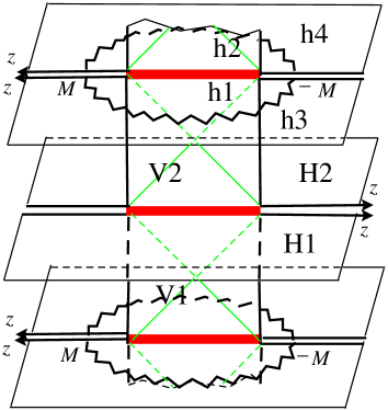
Figure 20: The subextremal Reissner-Nordstrøm card diagram. The ellipse singularity has semimajor axes $z=\pm M$ and $\rho=Q$, and the rod endpoints are the foci on the $z$-axis at $z=\pm\sqrt{M^{2}-Q^{2}}$.

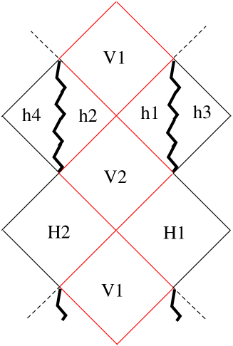
Figure 21: The extended Reissner-Nordstrøm Penrose diagram, including negative mass universes.

5.1.2 Extremal Reissner-Nordstrøm

Starting from the above card diagram we now examine the extremal limit $Q\to\pm M$. In this case the vertical cards which represent the regions between the two horizons get smaller and disappear. When $Q=M$, the horizontal cards are now only attached at point-like extremal-horizons and only half of the horizontal cards remain connected, see Fig. 22. The region near the point-horizons are anti-de Sitter throats although cards themselves cannot adequately depict the throat region. The throat is a ‘connected’ sequence of points on vertically adjacent horizontal cards.

Figure 22: Extremal RN horizontal cards are connected in an AdS₂ fashion at their origins. A side-view $z=0$ cross section is also shown.

To understand how to go beyond the horizon, it is important to remember that there were special null lines inside the black hole. In the extremal case the foci for the null lines become degenerate. In passing a special null line, we use the opposite branch of the square root for the Minkowski distance to the focus. For extremal black holes, both foci degenerate, and so we change the sign of all occurrences of the square root when we pass through the throat. This is a result of the simple fact that for extremal Reissner-Nordstrøm the functions $R=R_{+}=R_{-}=r-M$ both become negative inside the horizon. Hence we change the sign of $R$ to continue past the point $\rho=z=0$ onto either of the two adjacent horizontal cards, which have a singularity in the form of a half circle.

For Majumdar-Papapetrou solutions, this ‘sign change rule’ agrees with that in [5]. For an axisymmetric array, one can then easily draw the interior regions on horizontal cards, and find negative-mass-object universes on their complements. The work of [5] of course holds for an arbitrary array.

5.1.3 Superextremal black holes

The superextremal $|Q|>|M|$ Reissner-Nordstrøm black hole does not have horizons or vertical cards. Its card diagram consists of two horizontal cards, connected along the segment $0\leq\rho\leq\sqrt{Q^{2}-M^{2}}$, $z=0$. One card has a semi-ellipse singularity passing through the points $(\rho=0,z=\pm M)$ and $(\rho=Q,z=0)$.

These two horizontal cards are connected in the same sense as a branched Riemann sheet. By choosing Weyl’s canonical coordinates (meaning $Z=\rho+iz$ with $-($Coef$\,dt^{2})($Coef$\,d\phi^{2})=($Re$\,Z)^{2}$), the solution is no longer accurately represented on the horizontal card. This can be seen by examining the coordinate transformation (37) from Schwarzschild coordinates to Weyl coordinates. The coordinate transformation from $(r,\theta)$ double covers the Weyl half plane $(\rho\geq 0,z)$. For fixed radius and varying $\theta$, the coordinates from $M<r<\infty$ cover the Weyl plane in semi-ellipses which degenerate to the segment $(0\leq\rho\leq\sqrt{Q^{2}-M^{2}},z=0)$, which serves as a branch cut. The range $-\infty<r<M$ again covers the half-plane with $r=0$ forming an ellipse singularity. Therefore the point $(\rho=\sqrt{Q^{2}-M^{2}},z=0)$ acts as a branch point with a branch cut segment running to the $z$-axis. In summary while for the subextremal black hole the cards are joined by a four card horizon along a line segment of length $2\sqrt{M^{2}-Q^{2}}$, superextremal black holes involve a horizontal card branch cut along a line segment of length equal to the ‘rod length’ $2\sqrt{Q^{2}-M^{2}}$.

This double cover of the Weyl plane can be mapped onto a singly covered space by taking the appropriate square root. By choosing a new coordinate $W=\sqrt{Z-\sqrt{Q^{2}-M^{2}}}$, we map both the positive and negative-mass universes into the region $({\rm Im}\,W)^{2}-({\rm Re}\,W)^{2}\leq\sqrt{Q^{2}-M^{2}}$ (see Fig. 23). The image of the $z$-axis boundary is a hyperbola where the $\phi$ circle vanishes. The origin $W=0$ is the image of the branch point and the image of the line segment $(0\leq\rho\leq\sqrt{Q^{2}+M^{2}},z=0)$ is a line connecting the two hyperbolas and intersecting the origin of the $W$-plane. In the $W$-plane the $z$-axis and $\rho$-axis are no longer orthogonal. Larger values of $\rho$ past the branch point are mapped to the real $W$-axis. The singular nature of $e^{2\gamma}\propto 1/R_{+}R_{-}\propto 1/|\Delta Z|\propto 1/|W|^{2}$ has been fixed by $e^{2\gamma}dZd\overline{Z}=4|W|^{2}e^{2\gamma}dWd\overline{W}$. Finally the black hole singularity is mapped to a curved segment stretching from one hyperbola line to the other, to the left of the branch cut.

Figure 23: The superextremal RN black hole, after conformal transformation to the $W$-plane. This is a branched, static horizontal card, with two boundaries and one branch point.

Alternatively one can use a Schwarz-Christoffel transformation to map the two universes onto the strip $|{\rm Im}\,W|\leq W_{0}$. This is useful when the horizontal card boundaries are horizons as it allows for multiple horizontal cards to be placed adjacent to each other at the horizons (Fig. 27). This technique of fixing a horizontal card with a branch point will also be used in more complicated geometries such as the hyperbolic representation of S-RN and multi-rod solutions in four and five dimensions.

Card diagrams distinguish between spacetimes which are ‘truly’ superextremal, $|Q|>|M|$, from those simply with $M<|Q|$. The superextremal card diagram of this section for example is different from a negative mass Schwarzschild card diagram which is only region h3, for example, of the subextremal card diagram of Fig. 21.

5.1.4 Kerr

Written in Weyl-Papapetrou form, the Kerr black hole is

$$ds^{2} = -f(dt-\omega d\phi)^{2}+f^{-1}(e^{2\gamma}(d\rho^{2}+dz^{2})+\rho^{2}d\phi^{2}),$$

$$f = \frac{(R_{+}+R_{-})^{2}-4M^{2}+{a^{2}\over M^{2}-a^{2}}(R_{+}-R_{-})^{2}}{(R_{+}+R_{-}+2M)^{2}+{a^{2}\over M^{2}-a^{2}}(R_{+}-R_{-})^{2}},$$

$$e^{2\gamma} = \frac{(R_{+}+R_{-})^{2}-4M^{2}+{a^{2}\over M^{2}-a^{2}}(R_{+}-R_{-})^{2}}{4R_{+}R_{-}},$$

$$\omega = \frac{2aM(M+{R_{+}+R_{-}\over 2})(1-{(R_{+}-R_{-})^{2}\over 4(M^{2}-a^{2})})}{{1\over 4}(R_{+}+R_{-})^{2}-M^{2}+a^{2}{(R_{+}-R_{-})^{2}\over 4(M^{2}-a^{2})})},$$

where $R_{\pm}=\sqrt{\rho^{2}+(z\pm\sqrt{M^{2}-a^{2}})^{2}}=r-M\pm\sqrt{M^{2}-a^{2}}\cos\theta$. The transformation to Boyer-Lindquist coordinates is $\rho=\sqrt{r^{2}-2Mr+a^{2}}\sin\theta$, $z=(r-M)\cos\theta$.

For $|a|<|M|$ the Kerr black hole card diagram (see Figure 24) is similar to Reissner-Nordstrøm except that the singularity is a point and lies at $\rho=a$, $z=0$ on each negative-mass card. The outer and inner ergospheres lie on the positive-and negative-mass cards and are both described by the curve $z^{2}=\alpha^{2}-(\alpha^{2}/a^{2}-1)\rho^{2}-\rho^{4}/a^{2}$ where $\alpha^{2}=M^{2}-a^{2}$. The boundary of the region with closed timelike curves is also described by a quartic polynomial in Weyl coordinates. On the vertical card, which has length $2\sqrt{M^{2}-a^{2}}$, there are two special null lines.

The $r=0$ surface in BL coordinates is a semi-ellipse $\rho^{2}/a^{2}+z^{2}/M^{2}=1$ on the negative-mass card; but it is not a distinguished locus on the card diagram. Attempting to make one loop around the ring in BL coordinates clearly does not make a loop in Weyl space. When a traveller passes ‘through’ the ring at $r=0$, he merely traverses this non-singular semi-ellipse. For example if we start at the point $(r=0,\theta)$ and then attempt to loop around the ring in BL coordinates we arrive at $(r=0,\pi-\theta)$. In Weyl space this trajectory only connects two points on the non-singular semi-ellipse by a segment and so does not enclose the singularity. The question as to what happens when we go through the $r=0$ region can be answered simply in Weyl coordinates. At minimum it is clear that we must fill out the rest of the horizontal plane. In our analysis of the Reissner-Nordstrøm black hole we extended past $r=0$ by simply going to negative values of $r$ which filled out the rest of the horizontal half plane. The key difference is that for Kerr the singularity is point-like and so it is clear that it is physically possible for an observer to enter this second asymptotically flat universe. Finally the question as to whether we identify universes gotten to by going through the disk from above or below, now becomes the question of do we identify parts of the negative-mass card, as we circle the ring singularity point. A card diagram for a charged Kerr-Newman solution can similarly be constructed.

Figure 24: The Kerr card diagram.

In examining the Reissner-Nordstrøm solution it was found that the Weyl card diagram smoothly interpolates between the different sub/super-extremal parameter ranges. We now check the card diagram for Kerr for various parameter values. For fixed mass, if the angular momentum of the black hole is increased, the horizon shrinks to a point at the extremal limit and disappears when we go above the extremal limit. Extending past the pointlike horizon in the extremal case is again accomplished by changing the sign of both $R_{\pm}=R$. At the same time the ring singularity at $\rho=a$ moves farther from the origin. Therefore when the horizon disappears, the singularity is separated by a finite distance in Weyl space. The superextremal Kerr solution is similar to the superextremal Reissner-Nordstrom black hole except that the ellipse singularity is replaced by a point, and the ‘ergospheres’ map to an $\infty$-looking locus centered at $W=0$. Decreasing the angular momentum to zero, the singularity moves towards the horizon which increases in length. However this limit is not smooth since when the angular momentum reaches exactly zero, the curvature singularity jumps from being a point to a segment on the card diagram, to fully cover the horizon.

The superextremal Kerr solution is similar to the superextremal RN, except that the ellipse singularity is replaced by a point ($z=0$), and the ergospheres map to an $\infty$-looking locus centered at $W=0$.

5.1.5 The Black Ring

The 5d black ring solution of [4] is

$$ds^{2} =-{F(x)\over F(y)}dt^{2}$$

$$+ {1\over A^{2}(x-y)^{2}}\left[F(x)\Big{(}(y^{2}-1)d\psi^{2}+{F(y)\over y^{2}-1}dy^{2}\Big{)}+F(y)^{2}\Big{(}{dx^{2}\over 1-x^{2}}+{1-x^{2}\over F(x)}d\phi^{2}\Big{)}\right]$$

where $F(x)=1-\mu x$, $F(y)=1-\mu y$, and $0\leq\mu\leq 1$. The coordinates $x$, $y$ are 4-focus coordinates (in the sense that polar coordinates have two foci and prolate coordinates have three; we are counting the focus at infinity) that parametrize a half-plane of Weyl space $\rho\geq 0$, $-\infty<z<\infty$:

$$\rho = {1\over A(x-y)^{2}}\sqrt{F(x)F(y)(1-x^{2})(1-y^{2})}$$

$$z = {(1-xy)(F(x)-F(y))\over 2A(x-y)^{2}}\ .$$

The foci are on the $z$-axis at $z=\pm\mu/2A$ and $z=1/2A$. The black ring horizon is also on the $z$-axis along $-\mu/2A\leq z\leq\mu/2A$. The $\phi$-circle vanishes along $z\leq-\mu/2A$ and $\mu/2A\leq z\leq 1/2A$, and the $\psi$-circle vanishes along $z\geq 1/2A$. Curves of constant $y$ value degenerate to the horizon line segment as $y\to-\infty$, and degenerate to the $(1/2A,\infty)$ line segment (better pictured with a conformally equivalent disk) for $y\to-1$. Curves of $x=$constant degenerate to the vanishing $\phi$-circle line segment for $x\to 1$ and to the left semi-line $-\infty<z<-\mu/2A$ for $x\to-1$.

The card diagram is easy to construct and is not much different from the four dimensional Schwarzschild case. Past $y=-\infty$ we can go to $y=+\infty$ and hence imaginary $\rho=i\rho^{\prime}$, and move up a $\mu/A\times\mu/A$ square with two special null lines. At the top of the square, at $y=1/\mu$ we have the curvature singularity. Continuing again to real $\rho$ and running $y$ down to $1$, we map out a (negative-mass) horizontal card. The locus $y=1$ is the semi-line $z>1/2A$. The space closes off here as the $\psi$-circle vanishes, but one may formally continue to make an ‘extended card diagram’ which is useful in several applications. Past $y=1$, we see that for fixed $x$, reducing $y$ down to $x$ makes a topological half-line in a vertical card with a special null line like the elliptic card representations of S-Schwarzschild. Then for $-1<y<x$, we traverse another vertical card, which we could attach to our original positive-mass horizontal card along $z>1/2A$ (see Fig. 25). Thus when $y$ runs down from $x$ on the extended real line, it traverses a topological line in a V(ertical)-H(orizontal)-V-H-V sequence of cards. These noncompact vertical cards would be physically relevant if $\psi$ were continued to be time.

Figure 25: An extended card diagram for the black ring, where we have continued past $y=$constant boundaries for $-1\leq x\leq 1$. A $y$-orbit is drawn curving through several cards. Only one of the vertical and horizontal cards are drawn at each four card V-H-H-V card junction to avoid too many overlapping figures.

The above assumed $-1\leq x\leq 1$. One can instead fix $-\infty<y<-1$ and continue $x$ past $1$ to find a square card above the line segment $\mu/2A<z<1/2A$. The top of this square is $x=1/\mu$ and if $\phi$ were time, this would be the curvature singularity of a black hole (in an expanding KK bubble). For $1/\mu<x<\infty$ we sweep out a negative mass card, for $-\infty<x<y$ we sweep up a noncompact vertical card, and for $y<x<-1$ we sweep down a noncompact vertical card to attach to our original card at $z<-\mu/2A$.

Note that when passing through the black ring horizon at $y=-\infty$, the Weyl conformal factor [4]

$$e^{2\nu}={1+\mu\over 4A}{Y_{23}\over R_{1}R_{2}R_{3}}\sqrt{Y_{12}\over Y_{13}}\sqrt{R_{2}-\zeta_{2}\over R_{3}-\zeta_{3}},$$

stays real; $R_{3}-\zeta_{3}$ and $Y_{13}$ go negative. As we pass the special null lines, explicit appearances of $R_{1}$ and $R_{2}$ in the Weyl functions $e^{2U_{i}}$, $e^{2\nu}$ change sign.

5.2 Spacelike Branes

5.2.1 S-Reissner Nordstrom: elliptic diagram

Adding charge to the Schwarzschild solution moves the singularity from a four card junction and leaves a horizon. Adding charge has a similar effect on the Schwarzschild S-brane. This has already been described previously in Sec. 2.3.3 in the case of the parabolic card representation. Turning to the S-RN elliptic card diagram, as shown in Figure 26, the S-RN elliptic card diagram is similar to the elliptic Schwarzschild S-brane except the singularity is now a hyperbola $(\rho^{\prime},\tau)=(|Q|\sinh\theta,-M\cosh\theta)$, and the negative-mass connected universe has a 4-card horizon qualitatively similar to the positive-mass connected universe. As we increase the charge the singularity moves further out from the $\tau$-axis but any $Q\neq 0$ gives the same qualitative diagram.

Figure 26: The elliptic S-RN card diagram. The singularity is a hyperbola which does not intersect a horizon.

5.2.2 S-Reissner-Nordstrøm: hyperbolic card diagram and branch points

The Witten bubble in four dimensions has three card diagram representations as a result of its large $SO(2,1)$ symmetry group. There are likewise three card diagrams for S-Reissner-Nordstrøm which is equivalent to the statement that there are three ways to Killing-parametrize the hyperboloid $Z^{2}-X^{2}-Y^{2}=1$ embedded in ${\bf R}^{2,1}$ where $dZ$ is timelike. The more well known ways to parametrize the hyperboloid are elliptic, where we group terms as $Z^{2}-(X^{2}+Y^{2})=1$ and this leads to two Weyl foci being real, and hyperbolic where $(Z^{2}-Y^{2})-X^{2}=1$ and the Weyl foci are both imaginary.

First let us recap in Boyer-Lindquist coordinates the Reissner-Nordstrøm solution is commonly written as

$$ds^{2} = -(1-2M/r+Q^{2}/r^{2})dt^{2}+(1-2M/r+Q^{2}/r^{2})^{-1}dr^{2}+r^{2}(d\theta^{2}+\sin^{2}\theta d\phi^{2}),$$

$$A = {Qdt\over r}\ .$$

If we send $t\to ix^{4}$, $M\to iM$, $r\to it$, $\theta\to\pi/2+i\theta$, and $\phi\to i\phi$ then we get the solution

$$ds^{2} = (1-2M/t-Q^{2}/t^{2})(dx^{4})^{2}-(1-2M/t-Q^{2}/t^{2})^{-1}dt^{2}+t^{2}(d\theta^{2}+\cosh^{2}\theta d\phi^{2}),$$

$$A = {Qdx^{4}\over t}.$$

Here we leave $\phi$ noncompact so the ranges on the coordinates are $-\infty<\tilde{\theta}<\infty$, $-\infty<\phi<\infty$ and take the following embedding

$$X=\sinh\theta,\qquad Y=\cosh\theta\sinh\phi,\qquad Z=\cosh\theta\cosh\phi\ .$$

We see that the metric $d\theta^{2}+\cosh^{2}\theta d\phi^{2}$ has a 1-1 map onto the hyperboloid $Z^{2}-X^{2}-Y^{2}=1$ which is ${\bf H}_{2}$. Therefore this Wick rotation is the entire S-RN solution but just in a different coordinate system. In this solution it possible to compactify the $\phi$ direction to produce an orbifold of ${\bf H}_{2}$ and therefore the S-RN solutions as well. Euclideanized AdS₂ is just ${\bf H}_{2}$, so this orbifold puts it at a finite temperature. In these coordinates, there is no longer a Killing circle vanishing at $X=Y=0$. This means that there is a card diagram for S-RN that has no such boundaries.

Now let us turn to the construction of the hyperbolic card diagram representation for S-RN which has a branch point on the horizontal card. In Weyl coordinates the metric and gauge field for subextremal Reissner-Nordstrøm are given in (37). To obtain the hyperbolic S-RN analytically continue $M\to iM$, $t\to ix^{4}$ and $\phi\to i\phi$ and change branches $R_{-}\to-R_{-}$. In this case the special null lines, $R_{\pm}=\sqrt{\rho^{2}+(z\pm i\sqrt{M^{2}+Q^{2}})^{2}}=0$, will intersect the real manifold at only one point and so their zero will correspond to a branch point. From the definition of the functions $R_{\pm}$ these S-branes can be thought of as being sourced by rods which have been turned on their side in the imaginary $z$-direction. In this analytic continuation it is also necessary to replace all instances of $R_{-}$ by $-R_{-}$ in the functions $f$, $e^{2\gamma}$ and $A$ for reality as in the superextremal S-dihole II solution of Subsection 3.3. We now have $R_{-}=\overline{R_{+}}\equiv\overline{R}$; issues of branches are discussed shortly. The metric can be written

$$ds^{2} = -f(dx^{4})^{2}+f^{-1}(e^{2\gamma}(d\rho^{2}+dz^{2})+\rho^{2}d\phi^{2}),$$ (39)

$$f = {M^{2}+Q^{2}-({\rm Im}\,R)^{2}\over({\rm Im}\,R+M)^{2}},$$

$$e^{2\gamma} = {M^{2}+Q^{2}-({\rm Im}\,R)^{2}\over|R|^{2}},$$

$$A = {Q\,dx^{4}\over{\rm Im}\,R+M}.$$

In this case, on the horizontal card, $x^{4}$ is a timelike coordinate and $\phi$ is spacelike.

To understand how the branch point arises, let us examine the coordinate transformation from Schwarzschild to Weyl for the range $M\leq t\leq M+\sqrt{M^{2}+Q^{2}}$. Although we have Wick rotated the Schwarzschild coordinates to obtain the S-RN solution, the Weyl coordinates $\rho$ and $z$ are not Wick rotated. At a fixed value of $\theta>0$, the $t$-orbits are ellipses and there is a degenerate limit as $\theta\to 0$. In this limit the ellipse becomes the segment $z=0$, $0\leq\rho\leq\sqrt{Q^{2}+M^{2}}$ traced back and forth. We take this segment as the branch cut. Ellipses for $\theta<0$ fill out another copy of the horizontal half-plane.

The locus $t=M+\sqrt{M^{2}+Q^{2}}$ maps to the entire $z$-axis where there is a horizon which we call $\cal{H}_{+}$. Here it is possible to analytically continue $\rho\to i\rho^{\prime}$ and we find the usual four-card junction. The vertical cards are in the ‘positive mass’ S-RN universe. On the vertical cards, $f$ and $e^{2\gamma}$ are strictly negative and well-behaved; the coordinate $\rho^{\prime}$ is timelike while $x^{4}$, $z$ and $\phi$ are spacelike. These ‘positive-mass’ vertical cards have no singularities, no special null lines and no boundaries so the $\phi$-direction does not vanish and we may leave $\phi$ noncompact.

Using the same techniques as in the superextremal RN or Kerr cases it is possible to obtain a singly covered card by a conformal transformation. Henceforth the card diagram for S-RN will be drawn in the conformally-fixed coordinate $W$ but we will continue to label points using the $(\rho,z)$ coordinates. In the $W$-plane the branch cut maps to a line segment connecting the two horizons ${\cal H_{\pm}}$ and passing through the branch point. The $z$ and large-$\rho$ axes no longer appear orthogonal. A curvature singularity divides the horizontal card at $\rho^{2}=Q^{2}+{Q^{2}z^{2}\over M^{2}}$ or ${\rm Im}\,R+M=0$. Extending past the singularity we reach a second horizon ${\cal H}_{-}$ (at $z<0$ with the standard branch prescription). The vertical cards here are in the ‘negative-mass’ universe. These are qualitatively similar to the positive mass ones and have no singularities, no boundaries, and no special null lines. The difference between going towards ${\cal H}_{+}$ and ${\cal H}_{-}$ is we must replace $R\to-R$ in (39) which affects the denominators of $f$ and $A$, and is equivalent to $M\to-M$ and $A\to-A$.

It is easy to take the chargeless limit $Q\to 0$ and we get the S-Schwarzschild solution where the curvature singularity coincides with the horizon ${\cal H}_{-}$.

The full S-RN card diagram is drawn in Fig. 27. The images of $\rho=0$ become two horizons ${\cal H}_{+}$ and ${\cal H}_{-}$, each being a copy of $-\infty<z<\infty$, $\rho=0$. The surface gravities are $\kappa_{\pm}=\sqrt{M^{2}+Q^{2}}/(\sqrt{M^{2}+Q^{2}}\pm M)^{2}$ at ${\cal H}_{\pm}$.

Figure 27: Hyperbolic S-RN card diagram after transformation to the $W$-plane. There are no boundaries where spacelike Killing circles vanish. One may identify every other horizontal card. The singularities are closer to the ${\cal H}_{-}$ horizon and are farther from the ${\cal H}_{+}$ horizon.

Comparing the elliptic and hyperbolic representations of S-RN, the horizon to the positive-mass quarter-plane vertical card of the elliptic is the same as the horizon to the positive-mass half-plane vertical card of the hyperbolic; the left-edge boundary of the horizon of the elliptic is the center point of that of the hyperbolic but only at $\phi_{\rm hyp}=0$; both of these points are $X=Y=0$ of $Z^{2}-X^{2}-Y^{2}=1$. The line segment where the $\phi_{\rm ell}$ circle vanishes in the elliptic corresponds to the branch cut of the hyperbolic, but only at $\phi_{\rm hyp}=0$.

We point out two ways to get the S-Schwarzschild from the Witten bubble: One can either take $M\to iM$ which sends elliptic (hyperbolic) Witten $\to$ hyperbolic (elliptic) S-Schwarzschild respectively. Alternatively, one can turn a vertical card on its side which preserves elliptic/hyperbolicity.

Just as we took the hyperbolic Witten bubble on its side and got hyperbolic S-RN, we can take the vertical half-plane card diagrams for the Kerr bubble, S-dihole I, and superextremal S-Kerr and S-dihole II and apply the $\gamma$-flip to yield new spacetimes. These solutions are not identical to any previously described solutions and will be described in [14].

To achieve the E-RN solution, Wick rotate S-RN by $Q\to iQ$; we will discuss the superextremal E-RN card diagrams below.

5.2.3 S-Kerr

The twisted S-brane [24], see also [25], is also known as S-Kerr, and is another example of a nonsingular time-dependent solution. It can be obtained from the Kerr black hole by analytically continuing the Boyer-Lindquist coordinates $r,t,\theta$ and the parameters $a,M$. For the parameter range $|a|<|M|$ there are horizons and the global spacetime has a unique representation as a series of cards connected in the same manner as the elliptic bubble (see Fig. 9) except the vertices ending the horizons are at $\tau=\pm\sqrt{M^{2}-a^{2}}$. The image of the ergosphere lies on the horizontal card and has the same qualitative shape as it does for the Kerr black hole diagram. The whole spacetime is connected and each horizon is a 4-card junction which we can extend to obtain an infinite number of distinct cards; it is possible to truncate to a finite number of distinct cards by suitably identifying cards. In comparison the Penrose diagram of the $z,t$ plane is in Fig. 28.

Figure 28: Subextremal $|a|<|M|$ S-Kerr Penrose diagram. V_± map to vertical cards of positive and negative ‘mass,’ while all H diamonds give identical horizontal cards. It is possible to identify cards (say, every other H diamond) so there are only a finite number of regions in the spacetime.

In the extremal limit $|a|\to|M|$, $\theta$-orbits on the vertical card shift up relative to the special null line, and any fixed ($t$, $\theta$) point is sent above the null line. The region below the null line disappears in this limit and the horizontal card collapses to a point. Furthermore, those geodesics in the upper-right card can only reach the lower-left card (and the same with upper-left and lower-right), splitting the universe into connected $45^{\circ}$ wedges just like the parabolic representation for the Witten bubble (Fig. 12), where the connections for dS₂ were added for clarity.

The case $|a|>|M|$ for S-Kerr does not have horizons and can be represented as a single vertical half plane card with $\rho\geq 0$ and with no special null lines. As we send $|a|\to|M|$, the $\theta$-orbits pull away from $\tau=0$ and the spacetime gets put into two wedges, $\rho<|\tau|$ with $d\tau$ timelike; this again gives the extremal card diagram discussed above. Finally in the limit where $|a|\to\infty$, the $\theta$-orbits flatten out and the solution becomes flat space.

5.2.4 5d Schwarzschild and Reissner-Nordstrøm, and S-variants

The Weyl Ansatz has been extended to higher dimensions. In this and the next subsection we discuss charged black holes, Witten bubbles and S-Schwarzschild solutions in five dimensions. Although most of the properties will be the same there will be some important differences regarding the card diagrams. A discussion on a charged Weyl Ansatz in higher dimensions is included in the appendix.

To begin with, the five dimensional Schwarzschild black hole can be written in the generalized Weyl Ansatz [4] and has a card diagram which is similar to the connected positive-mass universe of the four dimensional case. To fit the Weyl Ansatz the three sphere is parametrized as $d\theta^{2}+\sin^{2}\theta d\phi^{2}+\cos^{2}\theta d\psi^{2}$. There are two half-plane horizontal cards representing asymptotically flat regions and two vertical square cards $-\mu/4\leq z\leq\mu/4$ inside the horizon. Even though the card diagram is similar to the four dimensional case, however, the $z$-axis plays a different role. In the five dimensional case the boundary the $z$-axis where $z>\mu/4$ and the right boundary of the vertical square which it connects to, are both where the $\phi$-circle vanishes. The $z$-axis where $z<-\mu/4$ and the left boundary of the square is where the $\psi$-circle vanishes.

As discussed in the appendix, the Weyl formalism also holds in the presence of an electrostatic potential, so the charged five dimensional black hole of [39]

$$ds^{2}=-\Big{(}1-{\mu\over r^{2}}+{Q^{2}\over 4r^{4}}\Big{)}dt^{2}+\Big{(}1-{\mu\over r^{2}}+{Q^{2}\over 4r^{4}}\Big{)}^{-1}dr^{2}+r^{2}d\Omega_{3}^{2}$$

can be put into Weyl’s coordinates and a card diagram can be drawn. In this choice of units $Q=\mu$ is extremal. Now the coordinate transformation from the above Schwarzschild coordinates to Weyl coordinates is

$$\rho={1\over 2}\big{(}1-{\mu\over r^{2}}+{Q^{2}\over 4r^{4}}\big{)}^{1/2}r^{2}\sin 2\theta,\qquad z={1\over 2}(r^{2}-{\mu\over 2})\cos 2\theta.$$

As in the four dimensional black hole solutions, the charge $Q$ does not enter in the definition of the $z$-coordinate.

The card diagram is similar to that of the four dimensional Reissner-Nordstrøm in Fig. 21 except the foci are at $z={1\over 4}\sqrt{\mu-Q^{2}}$ and the singularity is a semi-ellipse passing through the points $(\rho,z)=(0,\pm\mu/4)$ and $(\rho,z)=(|Q|/4,0)$ on a horizontal card. It is again possible to attach a negative mass universe to the singularity to fill out the rest of the horizontal plane. Since Weyl coordinates depend only on $r^{2}$, filling out the rest of the horizontal card unambiguously take us to imaginary values of $r$ and not negative values of $r$.

To obtain the charged five dimensional Witten bubble, analytically continue the solution with $t\to ix^{5}$, $\phi\to i\phi$, $Q\to iQ$. This analytic continuation gave the elliptic representation of the Witten bubble in four dimensions. There is a quarter-plane vertical card above the $\phi$ ray with an $x^{5}$ vertical boundary; this boundary continues on a segment of the nonsingular horizontal card, and then there is a $\psi$ boundary.

To obtain the five dimensional S-RN, take the vertical card from the Witten bubble and turn it on its side using our flip $\gamma\to\gamma+i\pi$. This vertical card now has a $\phi$ boundary and an $x^{5}$ horizon. Continuing onto the horizontal card, the $\phi$ boundary terminates after a segment and at $r=0$, there is the S-brane singularity which maps to a hyperbola on the card. Past the singularity we complete the horizontal card with a negative mass universe. The rest of the $z$-axis is filled out by an $x^{5}$ horizon which is a four card junction. In short the card diagram looks just like the four dimensional case, except there is a nonvanishing spacelike $\psi$-direction which is of course not evident on the diagram.

5.2.5 Multiple representations in 5d and ${\bf H}_{3}$

As discussed in Section 2.3 the four dimensional S-RN and charged Witten bubble have three card representations which corresponds to the three difference ways of putting a Killing congruence on ${\bf H}_{2}$. In contrast, the five dimensional S-RN and charged Witten bubbles have 2 representations because there are only two ways to put two orthogonal Killing congruences on ${\bf H}_{3}$. The elliptic and parabolic card diagrams in four dimensions will be analogous to what will call elliptic-hyperbolic and parabolic-parabolic diagrams in five dimensions.

The standard representation of five dimensional S-RN involves parametrizing ${\bf H}_{3}$ by $ds^{2}=d\theta^{2}+\cosh^{2}\theta d\psi^{2}+\sinh^{2}\theta d\phi^{2}$ or

$$W^{\prime}=\cosh\theta\cosh\psi,\qquad Z=\cosh\theta\sinh\psi,\qquad X=\sinh\theta\cos\phi,\qquad Y=\sinh\theta\sin\phi,$$

where $-W^{\prime 2}+Z^{2}+X^{2}+Y^{2}=1$ and $dW^{\prime}$ is timelike.

It is a fact, which we will not prove here, that the isometries of ${\bf H}_{3}$ are precisely the conformal isometries of its conformal infinity, the Riemann sphere $S^{2}$ [28]. This is the complex Möbius group $PSL(2,{\bf C})$. To see the relation between ${\bf H}_{3}$ and $S^{2}$ in the above representation, send $\theta\to\infty$ to achieve $-W^{\prime 2}+Z^{2}+X^{2}+Y^{2}=0$ modulo rescaling. Then set $W^{\prime}=1$ to get $Z^{2}+X^{2}+Y^{2}=1$. A conformal isometry of $S^{2}$ induces an isometry of ${\bf H}_{3}$ and in simple cases it is easy to guess which Möbius transformation corresponds to which isometry. In the present example, $Z=\tanh\psi$, $X={\rm sech}\,\psi\cos\phi$, and $Y={\rm sech}\,\psi\sin\phi$. So the hyperbolic $\psi$ boost isometry corresponds to $z\to(1+\epsilon)z$ on $S^{2}$, whereas the elliptic $\phi$ azimuthal rotation isometry corresponds to $z\to e^{i\epsilon}z$ on $S^{2}$. It is easy to see that the only other pair-type of orthogonal Möbius transformations is perpendicular parabolic ones, $z\to z+\epsilon$ and $z\to z+i\epsilon$, and that this gives the only other pair-type of orthogonal Killing congruences on ${\bf H}_{3}$. For the half-3-space representation of ${\bf H}_{3}$ with coordinates $(x,y,1/\sigma>0)$ and metric $d\sigma^{2}/\sigma^{2}+\sigma^{2}(dx^{2}+dy^{2})$, these are just translations in $x$ and $y$.

The parabolic-parabolic representation of five dimensional S-RN is

$$ds^{2} = f_{5}(dx^{5})^{2}+f_{x}(dx)^{2}+f_{y}(dy)^{2}+e^{2\nu}(-d\rho^{\prime 2}+dz^{2}),$$

$$e^{2\nu} = t^{2}/(\mu^{2}-Q^{2})\sigma^{2},$$

$$f_{5} = 1-\mu/t^{2}+Q^{2}/4t^{4},$$

$$f_{x}=f_{y} = t^{2}\sigma^{2},$$

where $\rho^{\prime}=\sigma^{2}\sqrt{\mu^{2}-Q^{2}}(\sinh\zeta)/2$, $z=\sigma^{2}\sqrt{\mu^{2}-Q^{2}}(\cosh\zeta)/2$, and $t^{2}-\mu=\sqrt{\mu^{2}-Q^{2}}(\cosh\zeta)/2$, written for $t\geq t_{+}$. The card diagram looks like the parabolic representation of 4d S-RN.

Applying the $\gamma$-flip on the vertical wedge card of S-Schwarzschild we get the parabolic-parabolic Witten bubble. At the pointlike tip, we attach one downward-facing copies of that wedge in a dS₃ fashion.

There are no five dimensional analogues of the hyperbolic S-RN and hyperbolic superextremal E-RN (see next subsection) card diagrams. For all these solutions, the lack of a third card diagram in the five dimensional case can be understood from two different perspectives: the lack of a $z\to i\tau$ continuation in the Weyl functions $f_{x}$, $f_{y}$; or the restrictions on orthogonal congruences of ${\bf H}_{3}$.

5.2.6 Three representations for superextremal E-RN

Although it is not clear if E-brane solutions [40] should exist in a stable theory, they are interesting simple examples of new card diagrams. We examine the superextremal E-RN, $Q^{2}-M^{2}>0$, which can be obtained by starting from S-RN and continuing the charge $Q\to iQ$.

The elliptic representation can also be directly obtained from the RN black hole by continuing $t\to ix^{4}$, $r\to it$, $M\to iM$, $Q\to iQ$, and $\theta\to i\theta$. The elliptic representation for the superextremal E-brane Reissner-Nordstrøm solution is a vertical half-plane card with $\rho=\sqrt{Q^{2}-M^{2}}\cosh\zeta\sinh\theta$, $\tau=\sqrt{Q^{2}-M^{2}}\sinh\zeta\cosh\theta$, where $\zeta$ is defined as $t-M=\sqrt{Q^{2}-M^{2}}\sinh\zeta$. It has no special null lines and a singularity along a $\theta$-orbit at $t=0$ which forms a hyperbola in Weyl space.

The hyperbolic representation, achieved by instead sending $\theta\to\pi/2+i\theta$, and $\phi\to i\phi$ in BL coordinates gives an interesting card. The Weyl coordinates are $\rho^{\prime}=\sqrt{Q^{2}-M^{2}}\cosh\zeta\cosh\theta$, $z=\sqrt{Q^{2}-M^{2}}\sinh\zeta\sinh\theta$, so we have the relation $\rho^{\prime}\geq|z|+\sqrt{Q^{2}-M^{2}}$. Although $\rho^{\prime}$ is positive, the $z$ coordinate can take either sign; neither the $x^{4}$- nor the $\phi$-circle closes anywhere. The coordinates cover a vertical quarter-plane wedge with $\rho^{\prime}$ timelike. Extending past the null lines by reflection to make four wedges, the card becomes an entire vertical plane card. The two special null lines that meet at $\rho^{\prime}=\sqrt{Q^{2}-M^{2}}$ (see Figure 29).

This card diagram can be turned on its side to obtain a new solution the superextremal Witten E-bubble. By continuing $\tau\to iz$, the intersection of special null lines becomes the branch point of superextremal RN’s horizontal card. By considering complex $z$ and real $\rho$, one sees that quite generally, branch points on horizontal cards and intersecting special null lines on vertical cards are really the same thing.

Figure 29: Three representation for superextremal E-RN. The hyperbolic is a whole plane vertical card; there are two special null lines which meet at a point. This spacetime has the indicated singularity.

There is also a parabolic representation which is a noncompact vertical $45^{\circ}$ card, with $\rho>|\tau|$. Constant-$t$ loci are straight rays $\tau/\rho=$constant.

The superextremal Kerr-Newman E-Bubble with $Q^{2}-a^{2}-M^{2}>0$ has a card diagram structure like hyperbolic superextremal E-RN, except the naked singularity is replaced by an instantaneous S1-brane ring singularity, which appears as a point on the vertical card diagram, on the left wedge.

The five dimensional superextremal E-RN has two card diagram representations which look like the four dimensional elliptic and parabolic ones.

For the hyperbolic subextremal E-RN the card diagram is similar to the hyperbolic card diagram for S-RN except the singularity lies on the negative-mass vertical cards at $\rho^{\prime 2}=Q^{2}+{Q^{2}z^{2}\over M^{2}}$. For the extremal case $Q=M$, The horizontal card totally collapses and we take ourselves on the positive-mass vertical card. Now $R^{2}=z^{2}-\rho^{\prime 2}$, and the numerator of $f$ vanishes outside $\rho^{\prime}>|z|$; only consider this region. The spacetime is complete like extremal RN.

5.2.7 S-Black Rings

Starting from the black ring, one may try to continue $x\to ix$, $y\to iy$, and $\mu\to-i\mu$ in (5.1.5), in the hopes of finding a new time dependent S-Black Ring solution. Unfortunately there is a singularity which rides up the boundary of the vertical card and so the solution is nakedly singular. The problems seems to be that the horizon was adjacent to a singular boundary on the horizontal card. If we can find spacetimes where the horizon is adjacent to a regular boundary where a circle closes, then the vertical boundary on the vertical quarter-plane card must be nonsingular; that same circle will close with the same periodicity. To find such spacetimes, we eschew $xy$ coordinates and use Weyl methods.

One can define an S-black ring by taking the black ring’s two bubble solutions, with vertical quarter-plane cards either at $z<-\mu/2A$ or $z>1/2A$, and turn them on their sides. One finds four new extended card diagrams three of which are not nakedly singular. With the help of our description of the $xy$ parametrization of these cards, we can fill out the new card diagram structure which is the same as the extended black ring structure. The boundaries are labelled by the order of vanishing of $x^{5}$, $\phi$, $\psi$ as follows: $y=\pm 1$ is $(0,0,2)$, $x=\pm 1$ is $(0,2,0)$, $y=\infty$ is $(2,0,0)$, $x=\infty$ is $(-2,2,2)$, $y=1/\mu$ is $(-2,4,0)$, $x=1/\mu$ is $(2,-2,2)$. However all these spacetimes can be constructed directly using the procedure of [4] by prescribing singularities, boundaries, and acceleration/black hole horizons, and hence are not really new.

It is possible that some electrification or spinning generalization would yield less singular spacetimes with the same card diagram structure. If canonical card diagrams (or even more general card diagrams) do not apply, the card diagram structure of the vacuum Weyl solution is still useful as it gives us an approximation of the new global structure.

A quite interesting new five dimensional solution built using Weyl methods will be described in Section 6.3.

5.3 Israel-Khan solutions

Israel-Khan solutions[11] are arrays of black holes held apart by conical singularities or struts of pressure. Their Weyl representation is a series of rods along the $z$-axis. Their card representation is obtained by simply treating each separate rod as a horizon with a four card junction with two horizontal and two vertical cards. In particular special null lines still emanate from the foci of Weyl space, and a triangle is unfolded four times to give a square for each inner-horizon region. Because the function $f$ is multiplicative for each source of an Israel-Khan solution and because the singularities occur when $f=\infty$, the singularities lie at the top of the vertical square cards just as in the isolated black hole case.

Over connected parts of the boundary the conical excess angle is constant. In the case of two black holes physically this means that inside the left black hole’s horizon, two-spheres have conical excess singularities at their north poles, and inside the right black hole’s horizon, two-spheres have conical excess singularities at their south poles.

By taking the distance between them to zero, black holes can be made to merge in a discontinuous fashion. Adjacent square vertical cards go from having size $2m_{1}\times 2m_{1}$ and $2m_{2}\times 2m_{2}$ to size $2(m_{1}+m_{2})\times 2(m_{1}+m_{2})$. This parametric merging is not a physical process.

5.3.1 A 2-rod gravitational wave example

As an application of our Weyl techniques we examine the case of two rods neither of which will cross the real-$\tau$ line, similar to a situation considered in [19]. The rods have linear density $\lambda$ which need not be $1/2$, are centered at $z=\pm a$ and have length $2M$. The new step is to rotate the right rod counterclockwise in the complex $z$-plane and the left one clockwise. We rotate them by $90^{\circ}$. Using the standard branch cut the distances from the rod endpoints are

$$\tilde{r}_{1} = \sqrt{\rho^{2}+a^{2}-(\tau-M)^{2}+2ia(\tau-M)};{\rm\ distance\ to\ }z=-a+ib$$

$$r_{1} = \sqrt{\rho^{2}+a^{2}-(\tau+M)^{2}+2ia(\tau+M)};{\rm\ distance\ to\ }z=-a-ib$$

$$\tilde{r}_{2} = \sqrt{\rho^{2}+a^{2}-(\tau+M)^{2}-2ia(\tau+M)};{\rm\ distance\ to\ }z=a-ib$$

$$r_{2} = \sqrt{\rho^{2}+a^{2}-(\tau-M)^{2}-2ia(\tau-M)};{\rm\ distance\ to\ }z=a+ib.$$

Note that $\tilde{r}_{1}\leftrightarrow r_{2}$ and $\tilde{r}_{2}\leftrightarrow r_{1}$ under complex conjugation; this exchanges a point with its mirror across the $\tau$-axis. The Weyl function $f=e^{2U}$ is in this case

$$U_{\rm SLO}=\lambda\log{r_{1}+\tilde{r}_{1}+2iM\over r_{1}+\tilde{r}_{1}-2iM}\cdot{r_{2}+\tilde{r}_{2}-2iM\over r_{2}+\tilde{r}_{2}+2iM}$$ (40)

where both the numerator and denominator are real. The notation ‘S’ stands for ‘sum’ since the distances are summed $r_{1}+\tilde{r}_{1}$ and $r_{2}+\tilde{r}_{2}$, ‘L’ stands for ‘log,’ and ‘O’ stands for ‘odd’ since the solution has $U$ odd in $\tau$. This is one branch choice but it is not the only good choice.

Alternatively we can change the branch of $r_{2}$ and $\tilde{r}_{2}$, or equivalently the orientation of the rod at $z>0$. (If we had kept $M_{1}$ and $M_{2}$ distinct, we could send $M_{2}\to-M_{2}$ everywhere it appears. We deduce that the equivalence must also hold for $\gamma$ from its PDEs sourced by $U$.) This makes the complex logarithm purely imaginary, so to obtain a sensible metric we send $\lambda\to-i\lambda$ and get

$$U_{\rm SAE}=\lambda\arg{r_{1}+\tilde{r}_{1}+2iM\over r_{1}+\tilde{r}_{1}-2iM}\cdot{r_{2}+\tilde{r}_{2}+2iM\over r_{2}+\tilde{r}_{2}-2iM}$$ (41)

where the product of fractions is unimodular. This solution has sums, the angular argument function and is even in $\tau$. This branch choice is seemingly good and produces a different even wave.

Thirdly we can have

$$U_{\rm DAO}=\lambda\arg{r_{1}-\tilde{r}_{1}+2iM\over r_{1}-\tilde{r}_{1}-2iM}\cdot{r_{2}-\tilde{r}_{2}-2iM\over r_{2}-\tilde{r}_{2}+2iM},$$ (42)

which involves differences, arg, and is odd in $\tau$. If one is careful to take a continuous branch of the argument, the function $U$ is smooth.

Lastly we can have

$$U_{\rm DLE}=\lambda\log{r_{1}-\tilde{r}_{1}+2iM\over r_{1}-\tilde{r}_{1}-2iM}\cdot{r_{2}-\tilde{r}_{2}+2iM\over r_{2}-\tilde{r}_{2}-2iM};$$ (43)

which involves differences, log, and is even in $\tau$. This function is problematic in that it is not asymptotically flat as $\tau\to\pm\infty$, but is nonsingular.

The function $e^{2\gamma}$ can be gotten from [5][11] by multiplying by $4\lambda^{2}$ and analytically continuing. It is smooth but does not have good asymptotic properties. Recall that $\gamma=\gamma_{11}+2\gamma_{12}+\gamma_{22}$, where $\gamma_{ij}$ is the interaction of the $i$’th rod with the $j$’th rod.

5.3.2 The C-Metric

A half-plane horizontal card for the C-metric has one finite rod to give a black hole, and one semi-infinite rod to represent an acceleration horizon. The full card diagram is then shown in Fig. 30 which shows that it is quite natural to identify the two black holes that are accelerating apart from “each other,” and that there is an Einstein-Rosen bridge from one horizontal card to the other [41].

One can similarly draw card diagrams for spacetimes with two acceleration horizons and black holes in between; these are $\phi\to it$, $t\to i\phi$ Wick rotations of Israel-Khan solutions.

Figure 30: The card diagram for the C-metric. It is quite natural to identify the two black holes.

6 2-Rod solutions without $z\to i\tau$

With a few techniques, one can find new S-brane solutions which are like deformations of the hyperbolic representation of S-RN by multiple rods and this will break the ${\bf H}_{2}$ symmetry of the geometry. The ease of constructing such solutions is the advantage of Weyl coordinates. In this analytic continuation we will stay on a horizontal card and we will not continue $z\to i\tau$.

6.1 One vertical rod, one horizontal rod

One can find a solution which is somewhat like the elliptic Witten bubble and somewhat like hyperbolic S-Schwarzschild by turning one rod and leaving the other one alone. This solution shows how Weyl solutions are specified by their rod sources and boundary information on a horizontal card.

Here we begin with a horizontal half-plane card. Let us label the Killing directions as $x^{4}$ (time), $\phi$ (space) in that order and label a boundary by $(m,n)$ where as $\rho\to 0$, the metric component $g_{44}=f\sim\rho^{m}$ and $g_{\phi\phi}\equiv\rho^{2}f^{-1}\sim\rho^{n}$. By definition we have the relation $m+n=2$. In this scheme a horizon is $(m,n)=(2,0)$, an ordinary boundary where the Weyl card ends is $(0,2)$, and a Schwarzschild black hole singularity is $(-2,4)$.

Next we specify a background boundary which is of type $(0,2)$ along the $z$-axis of the Weyl card. On top of this place a rod from $-M\leq z\leq M$ of Schwarzschild type $(+2,-2)$ and a second rod of type $(+2,-2)$ from $a-\mu\leq z\leq a+\mu$. These sources generate

$$f_{1}={R_{+}+R_{-}-2M\over R_{+}+R_{-}+2M},\qquad f_{2}={r_{+}+r_{-}-2\mu\over r_{+}+r_{-}+2\mu}$$

where $R_{\pm}=\sqrt{\rho^{2}+(z\pm M)^{2}}$ and $r_{\pm}=\sqrt{\rho^{2}+(z-a\pm\mu)^{2}}$. Turn the second rod on its side by the analytic continuation $\mu\to i\mu$, $r_{-}\to-r_{-}$, $x^{4}\to ix^{4}$, $\phi\to i\phi$ which is like the one used for the hyperbolic representation of S-RN. The function $f=f_{1}f_{2}$ is negative, the coordinate $x^{4}$ is timelike and the solution is ready to become a charged S-brane upon imaginary-$C$ electrification, see Appendix 6.4. Denoting $r=r_{+}=\overline{r_{-}}$, the solution has

$$e^{2\gamma_{11}} = \frac{(R_{+}+R_{-})^{2}-4M^{2}}{4R_{+}R_{-}},$$

$$e^{2\gamma_{22}} = \frac{\mu^{2}-({\rm Im}\,r)^{2}}{|r|^{2}},$$

$$e^{4\gamma_{12}} = \frac{R_{-}r_{+}+(z-M)(z-a+i\mu)+\rho^{2}}{-R_{-}r_{-}+(z-M)(z-a-i\mu)+\rho^{2}}\,\frac{-R_{+}r_{-}+(z+m)(z-a-i\mu)+\rho^{2}}{R_{+}r_{+}+(z+M)(z-a+i\mu)+\rho^{2}}$$

The function $\gamma_{12}$ is real as can be checked.

The effect of turning the rod on its side is to induce a branch point at $(\rho=\mu,z=a)$. Fixing this branch point by taking the appropriate square root, we find two boundaries, labelled $+$ and $-$, which are the images of the $z$-axis on the horizontal card. The $+$ boundary is uniformly affected by $(+2,-2)$ and the $-$ boundary is uniformly affected by $(-2,+2)$. This makes the $+$ boundary a sequence, of horizon $(2,0)$, singularity $(4,-2)$, and horizon $(2,0)$ from left to right. The $-$ boundary is $(-2,4)$, $(0,2)$, $(-2,4)$.

Let us recall two solution generating techniques. There is a ‘sign flip’ procedure which is applicable to four dimensional vacuum Weyl solutions where

$$U\to-U+\log\rho,\qquad\gamma\to\gamma-2U+\log\rho.$$ (44)

In Israel-Khan solutions, this replaces rods with space and space with rods. When rods are rotated parallel to imaginary $z$, the interpretation is less clear. The sign flip sends $(m,n)\to(2-m,2-n)$.

Another technique is Harrison’s third theorem [42] which sends

$$2U\to 2U-\mu_{H}\log\rho,\qquad 2\gamma\to 2\gamma-\mu_{H}2U+{\mu_{H}^{2}\over 2}\log\rho,$$ (45)

where $\mu_{H}$ is real. This changes the order of $f$’s vanishing near $\rho=0$ uniformly at all boundaries.

Performing the sign flip (44) and then Harrison’s third theorem with $\mu_{H}=2$ on our solution gives a $-$ boundary of orders $(2,0)$, $(0,2)$, $(2,0)$, and a $+$ boundary of orders $(-2,4)$, $(-4,6)$, $(-2,4)$. The $+$ boundary has two Schwarzschild singularities and a bad singularity where $f\propto\rho^{-4}$. In the case of the Schwarzschild and S-Schwarzschild solutions, we saw that singularities can be moved/created by adding charge. Here we change the singularities by imaginary-$C$ electrification. Setting $f=-e^{2\overline{U}}$, we get a RN singularity wherever $\tanh\overline{U}={C\over\sqrt{1+C^{2}}}$. For large enough positive $C$, the RN singularity then hugs the $+$ boundary and leaves the rest of the universe (with Witten bubble horizons on the $-$ boundary) connected. The card diagram is shown in Figure 31.

Figure 31: 4d electrified solution; two rods, one turned on its side.

6.2 Two vertical or imaginary-displaced rods

There are three basic rod configurations which give topological-line horizons and topological-line singularities. All of these configurations involve branch cuts from the boundary of the $\rho-z$ half-plane out to a branch point in the interior of the card.

First, place a horizontal rod from $z=-M+ib$ to $z=M+ib$, and place a mirror rod from $z=-M-ib$ to $z=M-ib$. Branch points now occur (for the distances $r_{\pm}=\sqrt{\rho^{2}+(z\pm M-ib)^{2}}$ to the upper rod endpoints, and their conjugates) at $z=\pm M$, $\rho=b$, and the standard square root branch cut gives us branch cuts along $z=\pm M$, $0\leq\rho<b$. Undoing the two branch cuts gives $2^{2}=4$ boundaries (which may be horizons, singularities, or true boundaries where a circle vanishes).

Second, place a vertical rod from $z=i(b-M)$ to $z=i(b+M)$ and a mirror rod from $z=-i(b+M)$ to $z=-i(b-M)$. There are branch points at $z=0$, $\rho=b-M$ and $\rho=b+M$. One branch cut runs out to $\rho=b-M$ and an independent branch cut runs out to $\rho=b+M$. Again undoing the branch cuts gives four boundaries.

Third, place a vertical rod from $z=-iM$ to $z=iM$ like the second representation of S-Schwarzschild. If we place two such rods, one displaced from along real $z$, we get two branch cuts and four boundaries.

The orientations of rods (reversing the sign of some $M$’s) and branches to all endpoints can be considered; there will always be some solution for $U$ which is real and involves the real logarithm. For brevity this will not be spelled out.

In all cases, rods must be given density $1/2$ (sourcing $U$) to generate a $\gamma$ such that $e^{2\gamma}$ blows up to order 1 at the branch point. This is necessary to get a nonsingular spacetime after conformally fixing the branches on the horizontal card. For the hyperbolic S-Schwarzschild, we know that a single rod generates a horizon (where $f=e^{2U}$ vanishes $\propto\rho^{2}$), and a singularity (where $f$ blows up $\propto 1/\rho^{2}$). For that case we had $ds^{2}\supset f(dx^{4})^{2}-f^{-1}\rho^{2}d\phi^{2}$ where $f<0$.

For the cases of two rods, each boundary has a $\pm$ status relative to each rod. The $++$ boundary has $f\propto\rho^{4}$, a $+-$ or $-+$ boundary has $f\propto 1$, and the $--$ boundary has $f\propto 1/\rho^{4}$. So for the third case of two vertical-in-$z$ rods crossing the $z$-axis, not continuing Killing directions, we have $ds^{2}\supset-f_{1}f_{2}dt^{2}+f_{1}^{-1}f_{2}^{-1}\rho^{2}d\phi^{2}$ where each $f_{1}$, $f_{2}$ is negative.

We perform the sign flip (44). Here, this gives $f\propto\rho^{-2},\rho^{2},\rho^{2},\rho^{6}$ on the $++$, $+-$, $-+$, $--$ boundaries. This is ready to be turned into a charged S-brane solution via a real-$C$ electrification (see the next subsection).

In this case, writing $f\to e^{2\overline{U}}$ for real $\overline{U}$ on the horizontal card, the electrified solution goes singular at the locus $\coth\overline{U}={C\over\sqrt{C^{2}-1}}$. Picking $C$ sufficiently negative, there are S-Schwarzschild singularities hugging around the $+-$ and $-+$ boundaries which are still horizons. Each has an associated connected 4-card spacetime which generalizes S-RN.

It is possible to get three S-Schwarzschild singularities and one horizon: Instead of the sign flip, we can utilize Harrison’s third theorem (45). Picking $\mu_{H}=2$, we get $f\propto\rho^{2},\rho^{-2},\rho^{-2},\rho^{-6}$ on the $++$, $+-$, $-+$, $--$ boundaries. This is ready to be turned into a charged S-brane solution via a real-$C$ electrification.

In this case we can pick $C$ sufficiently positive so there are S-Schwarzschild singularities hugging the $+-$, $-+$, and $--$ boundaries. The $++$ boundary is still a horizon. So this is like S-RN but the horizontal card has three disjoint singularities.

6.3 5d solution with two rods, one turned on its side

We now give a prescription for a non-nakedly singular 5d spacetime using two rods, one turned on its side. Write the Killing coordinates $x^{5}$, $\phi$, $\psi$ in that order. Say that part of the boundary has order $(m,n,p)$ if $f_{5}$, $f_{\phi}$, and $f_{\psi}$ vanish to orders $\rho^{m}$, $\rho^{n}$, and $\rho^{p}$. Of course $m+n+p=2$. Take Killing orders $(2,-2,2)$, $(0,0,2)$, and $(2,0,0)$ for $z<-M$, $-M<z<M$, and $M<z$. Add in a $(+0,+2,-2)$ rod of length $\mu$ centered at $z=a$ and turn it on its side. We then get (see Figure 32) a $+$ boundary of $(2,0,0)$, $(0,2,0)$, and $(2,2,-2)$. Note that the horizon is adjacent to a $\phi$-circle closing and its quarter-plane vertical card will be nonsingular. The $-$ boundary is $(2,-2,2)$, $(0,0,2)$, and $(2,0,0)$. Again its horizon is adjacent to the $\psi$-circle closing and its quarter-plane vertical card will be nonsingular. The singularities in this spacetime are confined to the horizontal card and they are related by trivial Killing rotation to $(-2,2,2)$ boundaries which are ordinary 5d black hole ones; so they are no more singular than the 5d S-Schwarzschild.

Figure 32: 5D solution; two rods, one turned on its side.

6.4 Appendix: Weyl Electrification

Weyl’s electrification procedure [43] can be applied to any Israel-Khan solution or Wick rotation thereof. Calling our old gravitational potential $\overline{U}$, the new one is given by

$$e^{-U} = {e^{-v}\over 2}\left(\Big{(}1+{C\over\sqrt{C^{2}-1}}\Big{)}e^{-\overline{U}}-\Big{(}{C\over\sqrt{C^{2}-1}}-1\Big{)}e^{\overline{U}}\right),$$ (46)

$$e^{2U} = e^{2v}-2Ce^{v}A+A^{2},$$

where $C\geq 1$ and $v$ are constants and $e^{2\gamma}$ does not change. Using the conformal symmetry of the Einstein-Maxwell system and the freedom to shift $\gamma$ by a constant we may take $v=0$. As applied to Schwarzschild of mass $M_{0}$, this generates Reissner-Nordstrøm of $C=M/Q$ where $M_{0}^{2}=M^{2}-Q^{2}$. As applied to S-Schwarzschild, since we had sent $t\to ix^{4}$ this generates an E-RN.

The point of (46) is that the Weyl cards of the spacetime do not change, but singularities move. Where $\overline{f}$ used to behave like $\rho^{\alpha}$, $f$ behaves like $\rho^{|\alpha|}$. So horizons stay horizons and Schwarzschild singularities become horizons. New singularities are generated where the quantity in parentheses vanishes, and generically this is to first order, generating Schwarzschild singularities.

For imaginary $C$,

$$e^{-U} = {e^{-v}\over 2}\left(\Big{(}1+{C\over\sqrt{C^{2}+1}}\Big{)}e^{-\overline{U}}+\Big{(}1-{C\over\sqrt{1+C^{2}}}\Big{)}e^{\overline{U}}\right),$$ (47)

$$e^{2U} = 1-2iCA+A^{2},$$

will turn the S-Schwarzschild into an S-RN. Any value of $C$ is then allowed. This transformation also charges the Witten bubble.

These electrifications seemingly do not generate superextremal solutions, which require a change in the card structure. (They have branch cuts instead of line segments.)

7 Discussion

In this paper we have examined the utility of the Weyl Ansatz and constructed an associated card diagram. The card diagram conveniently captures most of the interesting properties of a spacetime including its singularities, horizons, null infinity and some of its causal structure. The main technical details that one has to deal with regarding card diagrams seem to be analytic continuation of the coordinates, special null lines and the choice of the branch of a square root, and branch points.

Here we give a summary of the solutions we have discussed in this paper. The card diagrams correctly capture the different regions of the charged Reissner-Nordstrøm black hole and its various charged and chargeless limits, and its negative mass complement. We also analyzed the Kerr black hole and its singularity structure; the passage to the second asymptotic universe through $r=0$ is quite clearly depicted.

The Witten bubble and S-brane had three card diagrams since there were three choices of coordinates which were compatible with the Weyl Ansatz. The hyperbolic representations had no foci on the card diagram. In the case of the bubble the card diagram is a half-plane vertical card, while the S-Schwarzschild was more technically involved and had a branch point which we fixed with a conformal mapping. The elliptic representations were very similar and consisted of two foci and six individual cards. The main difference is that for the S-Schwarzschild, the left 4-card junction is not a horizon but a singularity. Finally the parabolic representation of the bubble was an infinite array of triangles connected pointwise while the S-Schwarzschild had a 6-card butterfly shape. This third representation has a useful representation of their null infinity.

The S-Schwarzschild can be obtained from the bubble in two ways. One may start with the bubble and analytically continue $M\to iM$ in Weyl coordinates. In this case the hyperbolic/elliptic/parabolic representation of the bubble maps to the elliptic/hyperbolic/parabolic representation of the S-brane. There was also a second way to relate these two solutions which we termed the $\gamma$-flip and which was conveniently visualized as a flip of the associated cards about a null line. This procedure maintains the number of Weyl foci on the card and so maps all bubbles to similarly labelled S-branes. The $\gamma$-flip provides a very simple and interesting way to relate Schwarzschild with the bubble and the S-brane. In fact all spacetimes related in this way by $\gamma$-flips can be simultaneously drawn together in a complexified Weyl spacetime diagram.

There are six S-dihole universes which we called $\cal{U}$, $\cal{U}_{\pm}$ and $\cal{E}$, $\cal{E}_{\pm}$. The three $\cal{U}$ universes were non-singular and had interesting near horizon scaling limits which we named $\cal{W}$. The $\cal{E}$ universes were singular on a so called ergosphere, represented the decay of two dimensional unstable objects, and ${\cal E}$ itself had an S-Melvin universe scaling limits. It was also previously noted that both the dihole and the S-dihole I solutions had Melvin scaling limits. The reason for this is that all these Melvin limits come from the same neighborhood of the complexified Weyl space. These solutions were then generalized to include new arrays as compared to those mentioned in [38]. The generalization includes allowing for black holes on the real time axis which gives dS₂ horizons with ${\cal W}$-type scaling limits, and we were even able to construct a periodic universe.

We also detailed multiple rod solutions such as black rings, S-black rings, the C-metric. New electrified 4d solutions and a 2-horizon vacuum rod 5d solutions were given. Gravitational wave solutions were shown to have several choices for branches.

Finally we turn to some comments on future work. As for the S-brane solutions we have presented here, it seems possible that the relationship between the general array solution and the Melvin scaling limit may have some connection to the discussion on the decay of unstable branes. In particular while the S-dihole is generally unstable and will decay, the decay time can be made as long as we wish by appropriately scaling the parameters. Also while we have now found an infinite array solution with horizons, there is still potentially much to understand regarding this solution and its exact relation to the rolling tachyon. Further investigation of this decay process, its relation to the work in Ref. [44] and the possibility of an open-closed string duality could prove interesting.

We hope the techniques herein and this method of visualization are helpful for keeping track of the numerous Wick rotations and mentally partitioning complicated spacetimes into simpler regions. Aside from being a useful way to describe spacetime structures, and follow their Wick rotations, card diagrams may have alternative uses. As discussed in [4], the higher dimensional Schwarzschild solutions cannot be written in Weyl form and so do not have Weyl card diagrams. However, card diagrams are more general than as described in this paper; the recently developed Weyl-Papapetrou formalism [9] for $D\geq 5$ will yield card diagrams. Furthermore card diagrams do not really require Weyl’s canonical coordinates. Spacetimes with Weyl-type symmetry and yet where Weyl’s procedure fails algebraically can still admit card diagrams. An example is the inclusion of a nonzero cosmological constant $\Lambda$, where a $\gamma$-flip changes the sign of $\Lambda$. We also hope that these methods, or their further generalizations, have even greater applicability than to the multitude of spacetimes already discussed.

Appendix A Appendix: Electrostatic Weyl Formalism

The formalism of [4] can be extended for general $D$ to include an electrostatic potential. This is somewhat surprising since the electromagnetic energy-momentum tensor

$$T_{\mu\nu}=F_{\mu\rho}F_{\nu}{}^{\rho}-{1\over 4}g_{\mu\nu}F^{2}$$

is traceless only in $D=4$ and so Einstein’s equations are more complicated. Nevertheless, a cancellation does occur and one may sum the diagonal Killing frame components of the Ricci tensor to achieve a harmonic condition.

Follow the notation of [4] and add a 1-form potential $A(Z,\overline{Z})dt$ where $t=x^{1}$ is timelike ($\epsilon_{1}=-1$) and all other $x^{i}$, $i=2,\ldots,D-2$ are spacelike (with $\epsilon_{i}=+1$). The metric takes the form

$$ds^{2}=-e^{2U_{1}}dt^{2}+\sum_{i=2}^{D-2}e^{2U_{i}}(dx^{i})^{2}+e^{2C}dZd\overline{Z},$$

from which we extract the frame metric

$$g_{\hat{\mu}\hat{\nu}}={\rm diag}(-1,+1,\ldots,+1)\oplus\left[\begin{array}[]{cc}0&1/2\\ 1/2&0\end{array}\right].$$

For $F=dA$ we have $F_{\hat{Z}\hat{t}}=-F_{\hat{t}\hat{Z}}=\partial A\,e^{-U_{1}-C}$ and $F_{\hat{\overline{Z}}\hat{t}}=-F_{\hat{t}\hat{\overline{Z}}}=\overline{\partial}A\,e^{-U_{1}-C}$, all other components vanishing. We compute $F^{2}=-8\partial A\overline{\partial}A\,e^{-2U_{1}-2C}$ and

$$T_{\hat{t}\hat{t}} = 2\partial A\overline{\partial}A\,e^{-2U_{1}-2C}$$

$$T_{\hat{i}\hat{i}} = 2\partial A\overline{\partial}A\,e^{-2U_{1}-2C}\quad(i\neq 1)$$

$$T_{\hat{Z}\hat{Z}} = -(\partial A)^{2}e^{-2U_{1}-2C}$$

$$T_{\hat{\overline{Z}}\hat{\overline{Z}}} = \overline{T_{\hat{Z}\hat{Z}}}$$

$$T_{\hat{Z}\hat{\overline{Z}}} = 0.$$

The field equations are $R_{\hat{\mu}\hat{\nu}}-{1\over 2}g_{\hat{\mu}\hat{\nu}}R=T_{\hat{\mu}\hat{\nu}}$; taking the trace, we get

$$R=-{4(D-4)\over D-2}\partial A\overline{\partial}A\,e^{-2U_{1}-2C}$$

and Einstein’s equations are then

$$R_{\hat{\mu}\hat{\nu}}=T_{\hat{\mu}\hat{\nu}}-{2(D-4)\over D-2}g_{\hat{\mu}\hat{\nu}}\partial A\overline{\partial}A\,e^{-2U_{1}-2C}.$$ (48)

Form the sum $\sum_{i=1}^{D-2}R_{\hat{i}\hat{i}}\epsilon_{i}$; the right side of (48) gives

$$(D-4)2\partial A\overline{\partial}A\,e^{-2U_{1}-2C}-{2(D-4)\over D-2}(D-2)\partial A\overline{\partial}A\,e^{-2U_{1}-2C}=0.$$

Hence (following (2.4)-(2.5) of [4]) we get

$$\partial\overline{\partial}\exp\left(\sum_{i=1}^{D-2}U_{i}\right)=0,$$

the Weyl harmonic condition.

One can add magnetostatic potentials along spatial Killing directions as well. We skip remaining details and give the equations. Let us assume $x^{1}$ is timelike and $x^{i}$ are spacelike for $i=2,\ldots,D-2$, the potential is $A_{\it 1}=\sum_{i=1}^{D-2}A_{i}dx^{i}$, and the metric is $ds^{2}=-e^{2U_{1}}(dx^{1})^{2}+\sum_{i=2}^{D-2}e^{-2U_{i}}(dx^{i})^{2}+e^{2\nu}(d\rho^{2}+dz^{2})$ and $w=\rho+iz$, $\partial_{w}={1\over 2}(\partial_{\rho}-i\partial_{z})$. Einstein’s equations are

$$\Delta U_{1} = {1\over 2}\Big{(}\sum_{i=1}^{D-2}(\nabla A_{i})^{2}e^{-2U_{i}}+{D-4\over D-2}\sum_{i=1}^{D-2}(\nabla A_{j})^{2}e^{-2U_{i}},$$

$$\Delta U_{k} = {1\over 2}\Big{(}-(\nabla A_{1})^{2}e^{-2U_{1}}-(\nabla A_{k})^{2}e^{-2U_{k}}+\sum_{i\neq k,1}(\nabla A_{i})^{2}e^{-2U_{i}}$$

$$\qquad-{D-4\over D-2}\sum_{i\neq 1}(\nabla A_{i})^{2}e^{-2U_{i}}+{D-4\over D-2}(\nabla A_{1})^{2}e^{-2U_{1}}\Big{)},$$

and

$$\partial_{w}\sum_{i=1}^{D-2}\nu=-2\rho(\sum_{i<j}\partial_{w}U_{i}\partial_{w}U_{j}+{(\partial_{w}A_{1})^{2}e^{-2U_{1}}\over 2}-\sum_{i=2}^{D-2}{(\partial_{w}A_{i})^{2}\over 2}e^{-2U_{i}}).$$

Maxwell’s equations are

$$\nabla\cdot\big{(}\nabla A_{i}e^{-2U_{i}}\big{)}.$$

All Laplacians and divergences are with respect to a flat 3d axisymmetric auxiliary space with coordinates $\rho,z$.

References

- [1]
- [2] E. Witten, “Instability Of The Kaluza-Klein Vacuum,” Nucl. Phys. B 195, 481 (1982).
- [3] M. Gutperle and A. Strominger, “Spacelike branes,” JHEP 0204, 018 (2002) [arXiv:hep-th/0202210].
- [4] R. Emparan and H. S. Reall, “Generalized Weyl solutions,” Phys. Rev. D 65, 084025 (2002) [arXiv:hep-th/0110258].
- [5] R. C. Myers, “Higher Dimensional Black Holes In Compactified Space-Times,” Phys. Rev. D 35, 455 (1987).
- [6] H. Weyl, Ann. Phys. (Leipzig) 54, 117 (1917).
- [7] R. Emparan and E. Teo, “Macroscopic and microscopic description of black diholes,” Nucl. Phys. B 610, 190 (2001) [arXiv:hep-th/0104206].
-
[8]
-
A. Papapetrou, Ann. Physik 12 (1953) 309;
-
A. Papapetrou, Ann. Inst. H. Poincaré A 4 (1966) 83.
-
- [9] T. Harmark, “Stationary and axisymmetric solutions of higher-dimensional general relativity,” arXiv:hep-th/0408141.
- [10] C. Charmousis and R. Gregory, “Axisymmetric metrics in arbitrary dimensions,” Class. Quant. Grav. 21 (2004) 527 [arXiv:hep-th/0306069].
- [11] W. Israel, K. A. Khan, “Collinear Particles and Bondi Dipoles in General Relativity,” Nuovo Cim. 33, 3611 (1964).
- [12] M. A. Melvin, Phys. Lett. 8 (1964) 65.
-
[13]
-
M. S. Costa and M. Gutperle, “The Kaluza-Klein Melvin solution in M theory,” JHEP 0103 (2001) 027, hep-th/0012072;
-
M. Gutperle and A. Strominger, “Fluxbranes in string theory,” JHEP 0108 (2001) 037, hep-th/0104136.
-
- [14] G. C. Jones and J. E. Wang, in preparation.
- [15] C. M. Chen, D. V. Gal’tsov and M. Gutperle, “S-brane solutions in supergravity theories,” Phys. Rev. D 66, 024043 (2002) [arXiv:hep-th/0204071].
- [16] M. Kruczenski, R. C. Myers and A. W. Peet, “Supergravity S-branes,” JHEP 0205, 039 (2002) [arXiv:hep-th/0204144].
-
[17]
-
J. E. Wang, “Spacelike and time dependent branes from DBI,” JHEP 0210 (2002) 037, hep-th/0207089.
-
C. P. Burgess, F. Quevedo, S. J. Rey, G. Tasinato and C. Zavala, “Cosmological spacetimes from negative tension brane backgrounds,” JHEP 0210 (2002) 028.
-
- [18] N. Ohta, “Intersection rules for S-branes,” hep-th/0301095.
- [19] G. Jones, A. Maloney and A. Strominger, “Non-singular solutions for S-branes,” [arXiv:hep-th/0403050].
- [20] W. B. Bonnor, “An Exact Solution of the Einstein-Maxwell Equations Referring to a Magnetic Dipole,” Zeitschrift für Physik 190, 444 (1966).
- [21] R. Emparan, “Black diholes,” Phys. Rev. D 61, 104009 (2000) [arXiv:hep-th/9906160].
- [22] L. Cornalba and M. S. Costa, “A new cosmological scenario in string theory,” Phys. Rev. D 66, 066001 (2002) [arXiv:hep-th/0203031].
- [23] A. Sen, “Rolling Tachyon,” JHEP 0204 (2002) 048, hep-th/0203211; “Tachyon Matter,” JHEP 0207 (2002) 065, hep-th/0203265; “Field Theory of Tachyon Matter,” Mod. Phys. Lett. A17 (2002) 1797, hep-th/0204143; “Time Evolution in Open String Theory,” JHEP 0210 (2002) 003, hep-th/0207105.
- [24] J. E. Wang, “Twisting S-branes,” JHEP 0405, 066 (2004) [arXiv:hep-th/0403094].
- [25] G. Tasinato, I. Zavala, C. P. Burgess and F. Quevedo, “Regular S-brane backgrounds,” JHEP 04 (2004) 038, hep-th/0403156.
- [26] H. Lu and J. F. Vazquez-Poritz, “Non-singular twisted S-branes from rotating branes,” arXiv:hep-th/0403248.
- [27] N. R. Sibgatullin, Oscillations and Waves in Strong Gravitational and Electromagnetic Fields, Springer-Verlag, Berlin Heidelberg 1991. (Originally published Nauka, Moscow 1984.)
- [28] K. Matsuzaki and M. Taniguchi, Hyperbolic Manifolds and Kleinian Groups, Oxford University Press, New York, 1998.
- [29] H. F. Dowker and S. N. Thambyahpillai, “Many accelerating black holes,” Class. Quant. Grav. 20, 127 (2003) [arXiv:gr-qc/0105044].
- [30] S. Chandrasekhar and B. C. Xanthopoulos, “Two Black Holes Attached To Strings,” Proc. Roy. Soc. Lond. A 423, 387 (1989).
- [31] E. Herlt, “Static and Stationary Axially Symmetric Gravitational Fields of Bounded Sources. I. Solutions Obtainable from the van Stockum Metric,” Gen. Rel. Grav. 9, No. 8, 711 (1978).
- [32] F. Dowker, J. P. Gauntlett, G. W. Gibbons and G. T. Horowitz, “The Decay of magnetic fields in Kaluza-Klein theory,” Phys. Rev. D 52, 6929 (1995) [arXiv:hep-th/9507143].
- [33] O. Aharony, M. Fabinger, G. T. Horowitz and E. Silverstein, “Clean time dependent string backgrounds from bubble baths,” JHEP 0207 (2002) 007, hep-th/0204158.
- [34] H. Stephani, D. Kramer, M. MacCallum, C. Hoenselaers, E. Herlt, Exact Solutions of Einstein’s Field Equations, 2nd ed., Cambridge University Press (2003).
- [35] A. Vilenkin, Phys. Rep. 121 (1985) 265.
- [36] R. Emparan and M. Gutperle, “From p-branes to fluxbranes and back,” JHEP 0112, 023 (2001) [arXiv:hep-th/0111177].
- [37] A. Maloney, A. Strominger and X. Yin, “S-brane thermodynamics,” JHEP 0310, 048 (2003) [arXiv:hep-th/0302146].
- [38] D. Gaiotto, N. Itzhaki and L. Rastelli, “Closed strings as imaginary D-branes,” Nucl. Phys. B 688, 70 (2004) [arXiv:hep-th/0304192].
- [39] K. D. Krori, T. Chaudhury, P. Borgohain, K. Das and C. R. Mahanta, “Charged Solutions In Higher Dimensions,” Can. J. Phys. 70, 752 (1992).
-
[40]
-
C. Hull, “Timelike T-duality, de Sitter space, large N gauge theories and topological field theory,” JHEP 9807 (1998) 021, hep-th/9806146; “Duality and the signature of space-time,” JHEP 9811 (1998) 017, hep-th/9807127;
-
V. Balasubramanian, J. de Boer and D. Minic, “Exploring de Sitter Space and Holography,” Class. Quant. Grav. 19 (2002) 5655, hep-th/0207245;
-
S. Bhattacharya and S. Roy, “Time dependent supergravity solutions in arbitrary dimensions,” JHEP 0312 (2003) 015, hep-th/030902.
-
- [41] S. W. Hawking, G. T. Horowitz and S. F. Ross, “Entropy, Area, and black hole pairs,” Phys. Rev. D 51, 4302 (1995) [arXiv:gr-qc/9409013].
- [42] B. K. Harrison, “New Solutions of the Einstein-Maxwell Equations from Old,” J. Math. Phys. 9 No. 11, 1744 (1968).
- [43] S. Fairhurst and B. Krishnan, “Distorted black holes with charge,” Int. J. Mod. Phys. D 10, 691 (2001) [arXiv:gr-qc/0010088].
-
[44]
-
A. Strominger, “Open string creation by S-branes,” Cargese 2002, Progress in string, field and particle theory p.335, hep-th/0209090;
-
B. Chen, M. Li and F. L. Lin, “Gravitational radiation of rolling tachyon,” JHEP 0211 (2002) 050, hep-th/0209222;
-
C. P. Burgess, P. Martineau, F. Quevedo, G. Tasinato and I. Zavala C., “Instabilities and particle production in S-brane geometries,” JHEP 0303 (2003) 050, hep-th/0301122;
-
F. Leblond and A. W. Peet, “SD-brane gravity fields and rolling tachyons,” JHEP 0304 (2003) 048, hep-th/0303035;
-
N. Lambert, H. Liu and J. Maldacena, “Closed strings from decaying D-branes,” hep-th/0303139;
-