SU-ITP 04-35

Dynamical Dimension Change
In
Supercritical String Theory

Simeon Hellerman¹ and Xiao Liu²

¹School of Natural Sciences, Institue for Advanced Study,
Princeton, NJ 08540
simeon@ias.edu

²Department of Physics and SLAC, Stanford University,
Stanford, CA 94309
liuxiao@itp.stanford.edu

We study tree-level solutions to heterotic string theory in which the number of spacetime dimensions $10+n$ changes dynamically due to closed string tachyon condensation. Taking the large-$n$ limit, we compute the amount by which the dilaton gradient $\Phi_{,X^{0}}$ changes during the condensation process. At leading order in $n$ we find that the change in the invariant magnitude of $\Phi_{,X^{0}}$ compensates the change in spacelike central charge on the worldsheet, so that the total worldsheet central charges are equal at early and late times. This result supports our interpretation of the worldsheet theory as a CFT of critical central charge which describes a dynamical reduction in the total number of spacetime dimensions.

1 Introduction

The simplest tree-level solutions to superstring theory in $D>10$ are the timelike linear dilaton backgrounds. For information on these, see [3], [2], [4], [5], [8].

These backgrounds posess the maximal Poincaré symmetry of the supercritical string, namely $D-1$ dimensional Poincaré symmetry of the spacelike directions. There is also an underlying $D$-dimensional Poincaré symmetry spontaneously broken only by the dilaton gradient, as pointed out by [8] and elaborated in [4], [5]. Since the time translation invariance is broken only by the dilaton, there is a time translation symmetry which acts on free string states but is broken by interactions.

In [2] a certain unstable heterotic string theory in $10+n$ dimensions was introduced, and it was argued that the ten-dimensional supersymmetric vacuum of SO(32) heterotic string theory could be reached as an endpoint of tachyon condensation in this theory. The argument was based on an approach to tachyon condensation which treated the worldsheet theory classically.

Under a classical scale transformation, the embedding coordinate ${X^{0}{}}$ shifts ${X^{0}{}}\to{X^{0}{}}+{\kappa Q}$, where $Q$ is the coefficient in the worldsheet coupling

$$\begin{array}[]{c}\Delta_{(linear~{}dilaton)}{\cal S}={Q\over{4\pi}}\int~{}d^{2}\sigma~{}\sqrt{g}~{}{\cal R}^{({2})}~{}{X^{0}{}},\end{array}$$ (1.2)

where ${\cal R}^{({2})}$ is the worldsheet Ricci scalar. This transformation leaves the action invariant up to terms independent of the Liouville field $X^{0}$, and hence does not affect the classical equations of motion.

Scale invariance is realized nonlinearly, in the sense that the scale transformation of the set of classical fields has a component which is zeroth order in the fields, as opposed to being entirely first order in the fields, as in a usual CFT. This realization of conformal invariance has the consequence that one can take an arbitrary scalar operator ${\cal O}_{(\Delta,\Delta)}$ of arbitrary weight $(\Delta,\Delta)$ and make it into a marginal operator by dressing it with an exponential ${\rm exp}\{2\beta{X^{0}{}}\}$, with the exponent $\beta$ adjusted to give exponential weight $(1-\Delta,1-\Delta)$. At the classical level the exponent is determined by the equation

$$\begin{array}[]{c}-Q\beta=1-\Delta.\end{array}$$ (1.4)

Quantum mechanically, the relationship is modified to

$$\begin{array}[]{c}-Q\beta+\beta^{2}=1-\Delta.\end{array}$$ (1.6)

Apart from this modification, the inclusion of quantum effects has other consequences for the theory.

Most important from our point of view is that the interpretation of the worldsheet theory as interpolating between two linear dilaton vacua with different dilaton gradients $Q_{\pm}$ as ${X^{0}{}}\to\pm\infty$ depends on quantum effects for consistency. Specifically, in order for the total central charge of the theory to be the same at ${X^{0}{}}\to+\infty$ as at ${X^{0}{}}\to-\infty$, the dilaton slope $Q$ must change in order to compensate the loss of ’matter’ central charge due to the perturbation by the dressed relevant operator ${\cal O}$. This cannot happen at the classical level. The aim of this paper is to illustrate the mechanism by which quantum effects renormalize the dilaton gradient $Q$ and keep the total central charge of the theory constant in both limits ${X^{0}{}}\to\pm\infty$.

2 A string worldsheet theory which interpolates between two linear dilaton CFT’s

Let us make this more concrete by reviewing the specific theory we will be analyzing. In this section we will focus on the classical analysis of the CFT. From this point of view it will be possible to see that the endpoint of closed string tachyon condensation will be a reduced number of spacetime dimensions. We will also explain why it is necessary to go beyond the classical analysis in order to see the dynamical readjustment of the dilaton gradient in target space time, which is necessary for the consistency of the CFT.

2.1 The type ${\rm HO}^{+({n})/}$ string in a linear dilaton background

We begin with a certain unstable heterotic string theory introduced in [2] and referred to as type ${\rm HO}^{+({n})/}$. The worldsheet theory is defined (in conformal gauge) by 9+n spacelike embedding coordinates $X^{i}$ and their right-moving worldsheet superpartners $\psi^{i}$, as well as a timelike embedding coordinate ${X^{0}{}}$ and its right-moving superpartner $\psi^{0}{}$. There are also 32+n left-moving fermions ${\tilde{\lambda}}^{a}$. All the worldsheet fields are free. To make the central charge critical, we consider the theory in a timelike linear dilaton background. On a flat worldsheet, the only effect of the linear dilaton is to add a term to the super-Virasoro generators which is linear in ${X^{0}{}},\psi^{0}{}$ rather than quadratic, and proportional to Q. The condition for critical central charge $(\tilde{c},c)^{matter}=(26,15)$ is

$$\begin{array}[]{c}4Q^{2}=n\end{array}$$ (2.8)

To preserve modular invariance we project onto states of even overall worldsheet fermion number $F_{W}$. With this projection there is a bulk tachyon $T^{a}$ living in the fundamental representation of $SO(32+n)$.

In order to stabilize the theory and relate it to conventional heterotic string theory HO with gauge group $SO(32)$ in ten dimensions, consider the ${\rm HO}^{+({n})/}$ string on an orbifold singularity, where the orbifold action is

$$\begin{array}[]{c}X^{i}\to-X^{i},\hskip 36.135pt\hskip 36.135pt\hskip 36.135pti=10,\cdots,9+n\cr\psi^{i}\to-\psi^{i},\hskip 36.135pt\hskip 36.135pt\hskip 36.135pti=10,\cdots,9+n\cr{\tilde{\lambda}}^{a}\to-{\tilde{\lambda}}^{a},\hskip 36.135pt\hskip 36.135pt\hskip 36.135pta=1,\cdots,32+n\end{array}$$ (2.12)

The effect of this orbifolding is to give the bulk tachyons Dirichlet boundary conditions at the singularity

$$\begin{array}[]{c}T^{a}=0~{}{\rm at}~{}X^{10}=X^{11}=\cdots=X^{9+n}=0\end{array}$$ (2.14)

The $+(n)$ referrs to the existence of $n$ extra spacetime dimensions, and the diagonal slash $/$ refers to the fact that the fermion states of the system are defined by projection onto states of even overall worldsheet fermion number $(-1)^{F_{W}}=+1$, rather than even right- and left-moving worldsheet fermion numbers separately, so the partition function for the fermions is the diagonal modular invariant. For further details of the ${\rm HO}^{+({n})/}$ string theory and its relation to the critical $SO(32)$ heterotic superstring, see [2].

2.2 Tachyon perturbation

2.2.1 Classical analysis

A tachyon background $T^{a}(X^{\mu})$ couples to the worldsheet as a superspace integral

$$\begin{array}[]{c}\int~{}d\theta~{}{\tilde{\lambda}}^{a}~{}T^{a}(X^{\mu})\end{array}$$ (2.16)

which in components amounts to a Yukawa coupling

$$\begin{array}[]{c}-i{\tilde{\lambda}}^{a}~{}T^{a}_{~{}~{},\nu}(X^{\mu})~{}\psi^{\nu}\end{array}$$ (2.18)

and a potential

$$\begin{array}[]{c}V(X^{\mu})=T^{a}(X^{\mu})T^{a}(X^{\mu})\end{array}$$ (2.20)

In order to be scale invariant at the classical level, the tachyon perturbation must satisfy

$$\begin{array}[]{c}-Q~{}T_{,{X^{0}{}}}^{a}(X^{\mu})=T^{a}(X^{\mu}).\end{array}$$ (2.22)

Since under classical scale transformations, the $X^{i}$ are inert, and $X^{0}$ shifts by $Q$, the equation above is just a condition for a perturbation to be marginal. The classical marginality equation is solved by

$$\begin{array}[]{c}T^{a}(X^{\mu})={\rm exp}\{\beta{X^{0}{}}\}~{}f^{a}(X^{i}),\end{array}$$ (2.24)

with $\beta=-{1\over Q}$ and $f^{a}$ an arbitrary set of functions of the spatial coordinates.

At the quantum level, the marginality condition is modified to

$$\begin{array}[]{c}\eta^{\mu\nu}T_{,X^{\mu}X^{\nu}}^{a}(X)-Q~{}T_{,{X^{0}{}}}^{a}(X)=T^{a}(X)\end{array}$$ (2.26)

For a tachyon profile of the form

$$\begin{array}[]{c}T^{23+i}(X)=\mu^{i}R_{i}:{\rm exp}\{\beta_{i}{X^{0}{}}\}~{}\sin\left(X^{i}/R_{i}\right):,~{}~{}~{}~{}~{}~{}~{}~{}i=10,\cdots,9+n\cr\cr T^{1}=T^{2}=\cdots=T^{32}=0,\end{array}$$ (2.30)

the condition is

$$\begin{array}[]{c}-\beta_{i}Q+{1\over 2}\beta_{i}^{2}=1-{1\over{2R_{i}^{2}}}\end{array}$$ (2.32)

for each $i\in\{10,\cdots,9+n\}$. In this paper we will simplify our discussion by focusing on the limit where all the $R_{i}$ are large. As $R_{i}\to\infty$, we have

$$\begin{array}[]{c}{1\over 2}\beta_{i}-{1\over{\beta_{i}}}=Q,~{}~{}~{}~{}~{}{\rm all}~{}i.\end{array}$$ (2.34)

In this limit the worldsheet action for the $X^{i},\psi^{i},$ and ${\tilde{\lambda}}^{a}$ is purely Gaussian, dressed with ${X^{0}{}}$-dependence. The classical limit is the one in which we take $Q\to\infty$, with $\beta_{i}\to-{1\over Q}$. We will fix our convention for the direction of time by taking $Q<0,\beta>0$ in which the dilaton is decreasing with time and the tachyon is increasing.

In the classical limit, the physics of the worldsheet at ${X^{0}{}}\to+\infty$ is clear: the worldsheet potential is

$$\begin{array}[]{c}V(X)=\sum_{i}(\mu^{9+i})^{2}~{}{\rm exp}\{2\beta{X^{0}{}}\}~{}(X^{9+i})^{2},\end{array}$$ (2.36)

$\beta=-{1\over Q}$. If we hold ${X^{0}{}}$ fixed and treat it as a background, the effect of the potential is to give masses to the supercritical embedding coordinates $X^{i},i=10,\cdots,9+n$, except for those coordinates whose corresponding mass parameters $\mu^{i}$ are exactly zero. The nonzero masses become infinitely large in the limit ${X^{0}{}}\to+\infty$. Likewise the fermions ${\tilde{\lambda}}^{23+i}$ and $\psi^{i}$ have large masses by virtue of their Yukawa couplings

$$\begin{array}[]{c}\mu^{i}{\rm exp}\{\beta{X^{0}{}}\}{\tilde{\lambda}}^{23+i}\psi^{i}.\end{array}$$ (2.38)

So in the limit ${X^{0}{}}\to+\infty$, the massive fields decouple in the Wilsonian sense, leaving the string propagating in a smaller number of spacetime dimensions, and with a smaller gauge group. In particular if all of the $\mu^{i}$ are nonzero, all $n$ of the extra embedding coordinates and their superpartners, and all $n$ of the current algebra fermions ${\tilde{\lambda}}^{a}$ decouple.

2.2.2 Classical limit versus central charge matching

By treating the worldsheet theory as classical this way, it was shown in [2] that the worldsheet field content and discrete gauge charge assignments in the limit ${X^{0}{}}\to+\infty$ are those of the spacetime-supersymmetric heterotic string with $SO(32)$ gauge symmetry. One limitation of this treatment is that one cannot see how the timelike dilaton gradient is reduced to zero in the critical vacuum as a result of tachyon condensation.

Indeed, it is trivial to show that the effective worldsheet theory at ${X^{0}{}}\to+\infty$ is exactly the same as that of the critical, spacetime-supersymmetric type HO string, modulo the question of the linear dilaton term. But that is the best one can do; at the level of classical field theory, eliminating the massive degrees of freedom just means setting them to zero classically. There is no way that this can possibly affect the linear dilaton coupling

$$\begin{array}[]{c}{Q\over{4\pi}}\int~{}d^{2}\sigma~{}\sqrt{g}~{}{\cal R}^{({2})}~{}{X^{0}{}}.\end{array}$$ (2.40)

In order for the central charge to be constant, we would need

$$\begin{array}[]{c}Q_{-}^{2}-n=Q_{+}^{2}-(n-\Delta n),\end{array}$$ (2.42)

where $Q_{\pm}$ is the limit of the dilaton gradient as ${X^{0}{}}\to\pm\infty$, and $\Delta n$ is the change in the number of spacetime dimensions, which from the worldsheet point of view is equal to the number of nonzero mass parameters $\mu^{i}$. At the classical level this central charge matching condition automatically fails if $\Delta n\neq 0$, since $Q_{+}=Q_{-}$ in the classical treatment.

3 Semiclassical analysis of the worldsheet theory

In this section we will discuss aspects of the worldsheet theory considered at the semiclassical level. We will explain the effect which gives rise to the dynamical readjustment of the dilaton slope and show some of the Feyman diagrams responsible for this effect.

3.1 Dilaton slope renormalization by worldsheet loop corrections

We would like to go beyond the classical treatment of the worldhseet theory, and see whether or not loop corrections to the effective dilaton gradient can make the central charge matching condition hold. By ’loop corrections’ and ’effective’ we are always referring to quantum effects on the worldsheet; we will always be ignoring worldsheets of $g>0$ and working at tree level in the spacetime sense.

Figure 1: Integrating out massive degrees of freedom gives rise to Feynman diagrams which renormalize the magnitude of the coupling $\sqrt{g}~{}{\cal R}^{({2})}~{}{X^{0}{}}$ in the worldsheet Lagrangian. In this diagram the solid lines are $X^{i},\psi^{i},$ and ${\tilde{\lambda}}^{23+i}$ fields, and the dotted line is a ${X^{0}{}}$ field.

Taking the limit in which the number $n$ of extra spacetime dimensions becomes large, we will find that the effect of integrating out the massive embedding coordinates and fermions will be to renormalize the effective dilaton gradient in such a way as to keep the total central charge constant, despite the fact that the central charge of the matter theory is reduced as $X^{0}\to\infty$. This will be our main result.

It is easy to see that there are Feynman diagrams which would give loop corrections to the effective dilaton slope. Expanding the potential term and Yukawa couplings to leading order in $\beta$ yields trilinear interactions between two massive fields and an ${X^{0}{}}$ field:

$$\begin{array}[]{c}{\cal L}_{o(\beta^{1})}=\beta{X^{0}{}}\sum_{i=10}^{9+n}\left[(\mu^{i})^{2}(X^{i})^{2}-i{\tilde{\lambda}}^{23+i}\psi^{i}\right]\end{array}$$ (3.44)

So one can construct Feynman diagrams where the massive fields run in a loop, with an ${X^{0}{}}$ line attached. In a nonsupersymmetric theory this would give rise to a potential for ${X^{0}{}}$, but the worldsheet supersymmetry guarantees that the potential for ${X^{0}{}}$ must vanish, as we will calculate explicitly later. The argument for this is simple: any Lorentz-invariant, supersymmetric effective potential term for ${X^{0}{}}$ must be of the form

$$\begin{array}[]{c}\int~{}d\theta~{}{\tilde{\lambda}}^{a}~{}f^{a}({X^{0}{}})\end{array}$$ (3.46)

But such a term would violate the discrete worldsheet gauge symmetry under which all the ${\tilde{\lambda}}^{a}$ are odd. Therefore any effective potential would have to have another odd field in it, such as one of the $X^{i}$ with $i=10,\cdots,9+n$, to compensate.

This argument holds only on a flat worldsheet. On the sphere, the curvature of the fiducial metric (which we will take to be the round metric of radius $R_{WS}$) breaks worldsheet supersymmetry. Since the limit $R_{WS}\to\infty$ is controlled by worldsheet supersymmetry, the term of order $R_{WS}^{2}$ in the effective action must vanish, but terms subleading in the volume of the worldsheet are still allowed. In particular it is possible to generate a ${X^{0}{}}$-dependent effective term which scales as $R_{WS}^{0}$, which can be written as

$$\begin{array}[]{c}{1\over{4\pi}}\int~{}d^{2}\sigma~{}\sqrt{g}~{}{\cal R}^{({2})}~{}\Phi_{1-loop}({X^{0}{}}).\end{array}$$ (3.48)

This term scales as $R_{WS}^{0}$ because the $R_{WS}^{2}$ in $\sqrt{g}$ is cancelled by the $R_{WS}^{-2}$ in ${\cal R}^{({2})}$.

In other words, the spacetime dilaton gets a direct renormalization from integrating out the massive fields, and that contribution to the spacetime dilaton can be extracted by fixing a large, positive background value of ${X^{0}{}}$, and extracting the $R_{WS}^{0}$ term in the effective action on the sphere.

3.2 Wavefunction renormalization of the ${X^{0}{}}$ field

We will find that there is a wavefunction renormalization of the ${X^{0}{}}$ coordinate which will also be important. Unlike the dilaton coupling, this is an ’extensive’ contribution to the effective action, by which we mean that it scales as $R_{WS}^{2}$ rather than $R_{WS}^{0}$. It cannot be extracted from an effective action evaluated for static ${X^{0}{}}$, so we must consider a background with infinitesimal nonstatic perturbations added to a static piece, in order to calculate it.

Figure 2: Integrating out massive fields renormalizes the kinetic term for the ${X^{0}{}}$ field.

We have not yet calculated the effective action $S_{eff}[{X^{0}{}},\psi^{0}{}]$ for the massless fields, but let us suppose we knew it, and extract the effective kinetic term for ${X^{0}{}}$ from the effective action. The most general effective action for ${X^{0}{}}$ allowed by the symmetries can be written in the form

$$\begin{array}[]{c}S_{eff}[{X^{0}{}},\psi^{0}{}]=\int~{}d^{2}\sigma~{}\kappa({X^{0}{}})(\vec{\partial}{X^{0}{}})^{2}+{\rm higher~{}derivatives}~{}+\psi^{0}{}~{}{\rm terms}.\end{array}$$ (3.50)

(The term with zero derivatives vanishes due to supersymmetry, as explained earlier.) To extract the kinetic term, expand around the static background ${X^{0}{}}={X^{0}{}}_{({0})}$ to second order in a plane-wave fluctuation. That is, let ${X^{0}{}}(\sigma)$ be given by

$$\begin{array}[]{c}{X^{0}{}}={X^{0}{}}_{({0})}+\epsilon~{}{\rm exp}\{i\vec{k}\cdot\vec{\sigma}\}+\epsilon{}^{*}~{}{\rm exp}\{-i\vec{k}\cdot\vec{\sigma}\},\end{array}$$ (3.52)

where $\epsilon$ is an infinitesimal parameter. Setting the background values of the fermions $\psi^{0}{}(\sigma)$ to zero and expanding in both $k$ and in $\epsilon,\epsilon{}^{*}$, the effective action is given by

$$\begin{array}[]{c}S_{eff}[{X^{0}{}}_{({0})}+\epsilon~{}{\rm exp}\{i\vec{k}\cdot\vec{\sigma}\}+\epsilon{}^{*}~{}{\rm exp}\{-i\vec{k}\cdot\vec{\sigma}\},0]=2\kappa({X^{0}{}})~{}{V_{WS}}~{}|\epsilon|^{2}\vec{k}^{2}+o(|\epsilon|^{3})+o(k^{4})\end{array}$$ (3.54)

where ${V_{WS}}$ is the volume of the worldsheet. So if we are given an effective action, we can extract $\kappa({X^{0}{}})=4\pi G_{{X^{0}{}}{X^{0}{}}}$ as

$$\begin{array}[]{c}\left.\kappa({X^{0}{}}_{({0})})={1\over{2{V_{WS}}}}{\delta\over{\delta\epsilon}}{\delta\over{\delta\epsilon{}^{*}}}{\delta\over{\delta k^{2}}}S_{eff}[{X^{0}{}}_{({0})}+\epsilon~{}{\rm exp}\{i\vec{k}\cdot\vec{\sigma}\}+\epsilon{}^{*}~{}{\rm exp}\{-i\vec{k}\cdot\vec{\sigma}\},0]~{}~{}\right|_{\epsilon=\vec{k}=0}\cr\cr~{}~{}~{}~{}~{}~{}~{}~{}~{}~{}~{}~{}~{}~{}~{}=\left.{1\over{8{V_{WS}}}}{\delta\over{\delta\epsilon}}{\delta\over{\delta\epsilon{}^{*}}}{\delta\over{\delta k^{a}}}{\delta\over{\delta k^{a}}}S_{eff}[{X^{0}{}}_{({0})}+\epsilon~{}{\rm exp}\{i\vec{k}\cdot\vec{\sigma}\}+\epsilon{}^{*}~{}{\rm exp}\{-i\vec{k}\cdot\vec{\sigma}\},0]~{}~{}\right|_{\epsilon=\vec{k}=0}\end{array}$$ (3.58)

4 Large-$n$ limit

4.1 Central charge matching condition in the large-n limit

We will consider the limit in which the total number of spacetime dimensions $10+n$ is large, and the dynamical reduction in the number of spacetime dimensions is $\Delta n\sim o(1)$. In fact we will begin by taking $\Delta n=1$; the extension to higher $\Delta n$ is trivial as long as $\Delta n/n$ is small.

In order to know what we would like the answer to be, let us expand the central charge matching condition to leading order in $n$. Since $Q_{-}$ is the value of the dilaton gradient which appears in the bare Lagrangian, we will use $Q$ and $Q_{-}$ interchangeably:

$$\begin{array}[]{c}Q\equiv Q_{-}=-{1\over 2}\sqrt{n}.\end{array}$$ (4.60)

In order for the central charge matching condition to hold in the large-$n$ limit, the effective dilaton slope $Q_{+}$ at large ${X^{0}{}}$ should be

$$\begin{array}[]{c}Q_{+}=-{1\over 2}\sqrt{n-\Delta n}\sim Q+{1\over 4}{{\Delta n}\over{\sqrt{n}}}+o\left({{(\Delta n)^{2}}\over{n^{3\over 2}}}\right).\end{array}$$ (4.62)

4.2 Feynman diagrams in the large-$n$ limit

Let us now determine which Feynman diagrams we will need to retain in order to compute the leading nontrivial correction to the dilaton gradient in the large-$n$ limit.

• The direct contribution to the dilaton gradient is a Feynman diagram with one external ${X^{0}{}}$ line. The one-loop contribution to this diagram has a single internal loop of massive matter connected to the external line by a trilinear interaction vertex, whose scales as $\beta\sim-{1\over Q}\sim 2n^{-{1\over 2}}+o(n^{-{3\over 2}})$ in the large-$n$ limit. Contributions with more than one loop are suppressed by higher powers of $\beta$ and are subleading in the large-$n$ limit.

• The wavefunction renormalization for ${X^{0}{}}$ comes from Feynman diagrams with two external ${X^{0}{}}$ legs. Again the leading contribution is a one-loop diagram with a massive internal loop connected to the external lines by trilinear vertices. This diagram is of order $\beta^{2}\sim 4n^{-1}$ in the large-$n$ limit. Redefining the ${X^{0}{}}$ field to make the effective kinetic term canonical will contribute an amount of order $\beta^{2}Q=o(\beta)=o(n^{-{1\over 2}})$ to the effective dilaton gradient in canonical target space coordinates. Since this effect is of the same order as the leading direct renormalization of $Q$, it must also be retained. Higher-loop kinetic term renormalizations contribute $o(\beta^{3}Q)=o(\beta^{2})=o(n^{-1})$ or less to the canonical dilaton gradient in the large-$n$ limit, so we ignore them.

• The one-loop diagrams with two external ${X^{0}{}}$ lines and a quartic vertex have the same $\beta$-scaling (and hence $n$-scaling) as the diagram with two trilinear vertices, but such diagrams do not contribute to the renormalization of the kinetic term; the kinematics of the diagram make the loop integral independent of the external momentum $\vec{k}$.

• As mentioned earlier, we will also restrict ourselves to the approximation in which the spatial wavelength of the tachyon in the supercritical dimension is infinitely long. In this approximation, the leading-order worldsheet potential perturbation is purely quadratic as a function of the massive fields $X^{i},\psi^{i},$ and ${\tilde{\lambda}}^{23+i}$. As a result, every interaction vertex has exactly two massive lines.

• If they existed, one-loop diagrams without massive lines would make contributions of the same order in $\beta$ as the diagrams we consider. But every tree-level interaction vertex has exactly two massive lines, so every loop diagram must contain at least one massive loop. For one-loop diagrams with only massless external lines, massless lines cannot appear internally.

• The noncontribution of massless internal lines at one loop means that we do not need to distinguish between 1PI and Wilsonian effective actions at leading order in $n$. When all internal lines are massive, the only effect of leaving internal modes with momenta below $E_{IR}$ fixed and integrating over them is a set of contributions to the effective action which scale with positive powers of $E_{IR}/M_{internal}$. Since $M_{internal}$ is proportional to $\mu~{}{\rm exp}\{\beta{X^{0}{}}_{({0})}\}$, such corrections vanish in the limit ${X^{0}{}}_{({0})}\to+\infty$ in which we will evaluate the effective action.

• Since the ${X^{0}{}}$ and $\psi^{0}{}$ degrees of freedom are essentially nondynamical for the purposes of the one-loop calculation we will do, the result will be independent of the details of operator ordering of the exponential ${\rm exp}\{\beta{X^{0}{}}\}$ appearing in the superspace integrand. Beyond one loop, the operator ordering of the exponentials inevitably becomes important.

• The operator ordering of the $(X^{i})^{2}$ terms does matter at one loop, but there is no ambiguity: the ordering is determined by supersymmetry. In particular, the $(X^{i})^{2}$ potential is a simple product, not normal-ordered, because it must be the square of the superpotential, which is linear in $X^{i}$. The singularity of the product of coincident fields is an exponential ${\rm exp}\{2\beta{X^{0}{}}\}$ with UV divergent coefficient. This singular term is cancelled by a second-order contact term between two insertions of the Yukawa coupling ${\rm exp}\{\beta{X^{0}{}}\}{\tilde{\lambda}}^{23+i}\psi^{i}$. This is just the standard cancellation of the one-loop vacuum energy in a supersymmetric system.

5 One-loop effects in the worldsheet theory

5.1 Comments on signatures

Since the kinetic term for the ${X^{0}{}}$ field is negative, the worldsheet action in Lorentzian signature clearly does not define a unitary quantum field theory. This is not bad in and of itself; ultimately we want to consider our 2D quantum theory as part of a string theory, in which the super-Virasoro constraits will eliminate the ${X^{0}{}}$ field as an independent degree of freedom, just as in critical string theory in a static background.

However since the nonunitary ${X^{0}{}}$ sector is in our case an interacting rather than a free theory, it is no longer clear that the path integral suffices to define it

Following [3] we would like to define our theories by Wick rotation from Euclidean space. In doing so it is necessary to assign the coordinate $X^{0}$ a minus sign under worldsheet time-reversal transformations. With this assignment, $X^{0}$ picks up a factor of $i$ under Wick rotation, and the Euclidean worldsheet action has positive definite kinetic term.

The result of this assignment is that the exponent $b$ appearing in the tachyon perturbation of the Euclidean worldsheet theory will be purely imaginary. The screening charge ${Q^{E}}$ appearing in the Euclidean action is imaginary as well. They satisfy the relation

$$\begin{array}[]{c}{1\over 2}b+{1\over b}\left(1-{1\over{2R^{2}}}\right)={Q^{E}},\end{array}$$ (5.64)

which goes to

$$\begin{array}[]{c}{1\over 2}b+{1\over b}={Q^{E}}\end{array}$$ (5.66)

in the long-wavelength limit $R\to\infty$. Note that this is the usual relationship between the ’screening charge’ ${Q^{E}}$ and the Liouville exponent $b$ for unitary super-Liouville theory. (Here, ${X^{0}{}}$ plays the role of the Liouville field.)

In the case of unitary Liouville theory (and the related sine-Liouville and super-sine-Liouville theories) $b$ and ${Q^{E}}$ are real, whereas in the action obtained by Wick rotating the Lorentzian worldsheet theory, $b$ and ${Q^{E}}$ are imaginary.

For our purposes we need not distinguish between the two cases, since we are working in perturbation theory. Indeed, amplitudes at fixed orders of perturbation theory are polynomial in $b$, we can treat arbitrary complex values of $b$ and ${Q^{E}}$ uniformly, always in the limit $|b|\to 0$. Doing so begs the question of whether or not the perturbative amplitudes we compute actually represent an asymptotic expansion to any exact amplitude in a nonperturbatively well-defined theory. Though important, this question must await an a priori nonperturbative definition of the theory, which we will not attempt here.

5.2 The action of (0,1) super-sine-Liouville theory

Since the massive fields couple to one another only through the ${X^{0}{}},\psi^{0}{}$ multiplet, it is clear that the one-loop amplitudes we consider are simply proportional to $\Delta n$, the number of massive fields. This need not be equal to $n$. In fact, we must keep $\Delta n=o(1)$ in order for all higher loops to be suppressed relative to the one-loop amplitudes.

Therefore we lose nothing by setting $\Delta n=1$. We will denote the massive boson, its superpartner, and the corresponding real current algebra fermion by $X,\psi^{X}{},$ and ${\tilde{\lambda}}$, respectively. The unique nonzero mass parameter, we shall denote by $\mu$.

The worldsheet action we are considering is the minimal $(0,1)$ supersymmetric extension of the bosonic theory known as sine-Liouville theory. While the minimal $(1,1)$ and $(2,2)$ supersymmetric versions of Liouville and sine-Liouville theory have been studied extensively, the minimal sine-Liouville theory with $(0,1)$ SUSY has gone unexplored. We now write down the Lorentzian and Euclidean actions for these theories.

5.2.1 Lorentzian action

We consider the minimal extension of the theory which admits right-moving (in Lorentzian signature) supercharge $\hat{{\cal Q}}_{+}=\hat{{\cal Q}}$. Then we define three SUSY multiplets as follows:

$$\begin{array}[]{c}\hat{{\cal Q}}{X^{0}{}}=-{i\over{\sqrt{2}}}\psi^{0}{},\hskip 36.135pt\hskip 36.135pt\hat{{\cal Q}}\psi^{0}{}=\sqrt{2}~{}\partial_{+}{X^{0}}{}\\ \\ \hat{{\cal Q}}X=-{i\over{\sqrt{2}}}\psi^{X}{},\hskip 36.135pt\hskip 36.135pt\hat{{\cal Q}}\psi^{X}{}=\sqrt{2}~{}\partial_{+}X\\ \\ \hat{{\cal Q}}{\tilde{\lambda}}=F\hskip 36.135pt\hskip 36.135pt\hat{{\cal Q}}F=-i\partial_{+}{\tilde{\lambda}}\end{array}$$ (5.72)

We can create a Lagrangian which is supersymmetric on a flat worldsheet up to a total derivative by acting on a ’superspace’ integrand ${\cal I}$ with $\hat{{\cal Q}}$ to get a lagrangian:

$$\begin{array}[]{c}{\cal I}\equiv-{{\sqrt{2}}\over{4\pi}}\psi^{0}{}\partial_{-}{X^{0}{}}+{{\sqrt{2}}\over{4\pi}}\psi^{X}{}\partial_{-}X+{1\over{4\pi}}{\tilde{\lambda}}F+{{\mu}\over{2\pi\sqrt{2}}}R~{}{\tilde{\lambda}}~{}{\rm exp}\{\beta{X^{0}{}}\}\sin(X/R)\\ \\ {\cal L}_{+-}\equiv\hat{{\cal Q}}\cdot{\cal I}\\ \\ =-{1\over{2\pi}}(\partial_{+}{X^{0}{}})(\partial_{-}{X^{0}{}})+{1\over{2\pi}}(\partial_{+}X)(\partial_{-}X)+{1\over{4\pi}}F^{2}\\ \\ -{i\over{4\pi}}\psi^{0}{}\partial_{-}\psi^{0}{}+{i\over{4\pi}}\psi^{X}{}\partial_{-}\psi^{X}{}+{i\over{4\pi}}{\tilde{\lambda}}\partial_{+}{\tilde{\lambda}}\\ \\ +{{\mu}\over{2\pi\sqrt{2}}}RF{\rm exp}\{\beta{X^{0}{}}\}\sin(X/R)\\ \\ +{{i\mu R\beta}\over{4\pi}}{\tilde{\lambda}}\psi^{0}{}{\rm exp}\{\beta{X^{0}{}}\}\sin(X/R)+{{i\mu}\over{4\pi}}{\tilde{\lambda}}\psi^{X}{}{\rm exp}\{\beta{X^{0}{}}\}\cos(X/R)\end{array}$$

where ${\cal L}_{+-}$ is the Lagrangian which gets integrated over $d\sigma^{+}d\sigma^{-}$. Integrating out the auxiliary field $F$ gives the lagrangian

$$\begin{array}[]{c}{\cal L}_{+-}=-{1\over{2\pi}}(\partial_{+}{X^{0}{}})(\partial_{-}{X^{0}{}})+{1\over{2\pi}}(\partial_{+}X)(\partial_{-}X)\\ \\ -{i\over{4\pi}}\psi^{0}{}\partial_{-}\psi^{0}{}+{i\over{4\pi}}\psi^{X}{}\partial_{-}\psi^{X}{}+{i\over{4\pi}}{\tilde{\lambda}}\partial_{+}{\tilde{\lambda}}\\ \\ -{{\mu^{2}R^{2}}\over{8\pi}}{\rm exp}\{2\beta{X^{0}{}}\}\sin^{2}(X/R)\\ \\ +{{i\mu R\beta}\over{4\pi}}{\tilde{\lambda}}\psi^{0}{}{\rm exp}\{\beta{X^{0}{}}\}\sin(X/R)+{{i\mu}\over{4\pi}}{\tilde{\lambda}}\psi^{X}{}{\rm exp}\{\beta{X^{0}{}}\}\cos(X/R)\end{array}$$

Note that there is no factor of $\beta^{2}$ in front of the bosonic potential.

Now we rewrite the action in the usual coordinates. That is, $\sigma^{\pm}\equiv\sigma^{0}\pm\sigma^{1}$, so $\partial_{\pm}={1\over 2}(\partial_{0}\pm\partial_{1})$. Further, ${\cal L}_{\sigma^{0}\sigma^{1}}=2{\cal L}_{\pm}$, so

$$\begin{array}[]{c}{\cal L}_{\sigma^{0}\sigma^{1}}={{\eta^{ab}}\over{4\pi}}\left[-(\partial_{a}{X^{0}{}})(\partial_{b}{X^{0}{}})+(\partial_{a}X)(\partial_{b}X)\right]\\ \\ +{i\over{4\pi}}\left[-\psi^{0}{}(\partial_{0}-\partial_{1})\psi^{0}{}+\psi^{X}{}(\partial_{0}+\partial_{1})\psi^{X}{}+{\tilde{\lambda}}(\partial_{0}+\partial_{1}){\tilde{\lambda}}\right]\\ \\ -{{\mu^{2}}\over{4\pi}}R^{2}{\rm exp}\{2\beta{X^{0}{}}\}\sin^{2}(X/R)\\ \\ +{{i\mu R\beta}\over{2\pi}}{\tilde{\lambda}}\psi^{0}{}{\rm exp}\{\beta{X^{0}{}}\}\sin(X/R)+{{i\mu}\over{2\pi}}{\tilde{\lambda}}\psi^{X}{}{\rm exp}\{\beta{X^{0}{}}\}\cos(X/R)\end{array}$$

For purposes of evaluating the massive fermion propagator, it is convenient to package the two Majorana-Weyl fermions $\psi^{X}{}$ and ${\tilde{\lambda}}$ into a single nonchiral Majorana fermion $\Psi\equiv\left(\matrix{\psi^{X}{}\cr{\tilde{\lambda}}}\right)$. We also abuse notation and use $\psi^{0}{}$ to denote the a two-component form of the Majorana-Weyl spinor $\psi^{0}{}^{\rm(one~{}component)}$ in which the right-moving component is constrained to vanish: from now on,

$$\begin{array}[]{c}\psi^{0}{}\equiv\psi^{0}{}^{\rm(two~{}component)}=\left(\matrix{\psi^{0}{}^{\rm(one~{}component)}\cr 0}\right).\end{array}$$ (5.91)

Then we can write the action as

$$\begin{array}[]{c}{\cal L}_{\sigma^{0}\sigma^{1}}={{\eta^{ab}}\over{4\pi}}\left[-(\partial_{a}{X^{0}{}})(\partial_{b}{X^{0}{}})+(\partial_{a}X)(\partial_{b}X)\right]\\ \\ +{i\over{4\pi}}\left[-\bar{\psi^{0}{}}\Gamma^{a}\partial_{a}\psi^{0}{}+\bar{\Psi}\Gamma^{a}\partial_{a}\Psi\right]\\ \\ -{{\mu^{2}}\over{4\pi}}R^{2}{\rm exp}\{2\beta{X^{0}{}}\}\sin^{2}(X/R)\\ \\ +{{i\mu R\beta}\over{2\pi}}\bar{\Psi}\psi^{0}{}{\rm exp}\{\beta{X^{0}{}}\}\sin(X/R)+{{i\mu}\over{2\pi}}\bar{\Psi}\Psi{\rm exp}\{\beta{X^{0}{}}\}\cos(X/R),\end{array}$$

where

$$\begin{array}[]{c}\bar{\Psi}\equiv-\Psi^{T}\Gamma^{0}\end{array}$$ (5.98)

and we use the basis

$$\begin{array}[]{c}\Gamma^{0}\equiv i\sigma^{2}=\left(\matrix{0&1\cr-1&0}\right),~{}~{}~{}~{}~{}~{}~{}~{}~{}~{}~{}~{}~{}~{}~{}\Gamma^{1}\equiv\sigma^{1}=\left(\matrix{0&1\cr 1&0}\right)\end{array}$$ (5.100)

Evaluated in the long-wavelength limit $R\to\infty$, the action becomes

$$\begin{array}[]{c}{\cal L}_{\sigma^{0}\sigma^{1}}={{\eta^{ab}}\over{4\pi}}\left[-(\partial_{a}{X^{0}{}})(\partial_{b}{X^{0}{}})+(\partial_{a}X)(\partial_{b}X)\right]\\ \\ +{i\over{4\pi}}\left[-\bar{\psi^{0}{}}\Gamma^{a}\partial_{a}\psi^{0}{}+\bar{\Psi}\Gamma^{a}\partial_{a}\Psi\right]\\ \\ -{{\mu^{2}}\over{4\pi}}{\rm exp}\{2\beta{X^{0}{}}\}X^{2}\\ \\ +{{i\mu\beta}\over{2\pi}}\bar{\Psi}\psi^{0}{}{\rm exp}\{\beta{X^{0}{}}\}X+{{i\mu}\over{2\pi}}\bar{\Psi}\Psi{\rm exp}\{\beta{X^{0}{}}\}.\end{array}$$

5.2.2 Euclidean action

In order to Wick rotate, we send $\partial_{0}\to i\partial_{0}$ and $\bar{\Psi}\to\Psi^{T}C{}^{*}$. As discussed earlier we also perform a change of dynamical variables ${X^{0}{}}\to i{X^{0}{}}$. ¿From this we obtain

$$\begin{array}[]{c}{\cal L}^{E}={{\delta^{ab}}\over{4\pi}}\left[(\partial_{a}{X^{0}{}})(\partial_{b}{X^{0}{}})+(\partial_{a}X)(\partial_{b}X)\right]\\ \\ +{i\over{4\pi}}\left[i\psi^{0}{}^{\rm T}C{}^{*}\Gamma^{a}\partial_{a}\psi^{0}{}+\Psi^{\rm T}C{}^{*}\Gamma^{a}\partial_{a}\Psi\right]\\ \\ +{{\mu^{2}}\over{4\pi}}{\rm exp}\{2b{X^{0}{}}\}X^{2}\\ \\ +{{i\beta\mu}\over{2\pi}}\Psi^{\rm T}C{}^{*}\psi^{0}{}{\rm exp}\{b{X^{0}{}}\}X+{{i\mu}\over{2\pi}}\Psi^{\rm T}C{}^{*}\Psi{\rm exp}\{b{X^{0}{}}\}.\end{array}$$ (5.111)

On a curved worldsheet, change the partial derivatives into covariant derivatives, and add the dilaton coupling:

$$\begin{array}[]{c}{\cal L}^{E}={{g^{ab}}\over{4\pi}}\left[(\partial_{a}{X^{0}{}})(\partial_{b}{X^{0}{}})+(\partial_{a}X)(\partial_{b}X)\right]+{i\over{4\pi}}\left[i\psi^{0}{}^{\rm T}C{}^{*}\Gamma^{a}\nabla_{a}\psi^{0}{}+\Psi^{\rm T}C{}^{*}\Gamma^{a}\nabla_{a}\Psi\right]\\ \\ +{{\mu^{2}}\over{4\pi}}{\rm exp}\{2b{X^{0}{}}\}X^{2}+{{i\beta\mu}\over{2\pi}}\Psi^{\rm T}C{}^{*}\psi^{0}{}{\rm exp}\{b{X^{0}{}}\}X+{{i\mu}\over{2\pi}}\Psi^{\rm T}C{}^{*}\Psi{\rm exp}\{b{X^{0}{}}\}\cr\cr+{{{Q^{E}}}\over{4\pi}}{X^{0}{}}~{}{\cal R}^{({2})}\end{array}$$ (5.116)

5.3 The one loop effective action for ${X^{0}{}}$

Computing the effective action for ${X^{0}{}}$ at one loop reduces to the computation of a determinant depending on the background configuration of ${X^{0}{}}$.

If the massive bosonic and fermionic degrees of freedom are represented as $B^{i}$ and $f^{i}$, respectively, then let their action in a given ${X^{0}{}}$ background be denoted by

$$\begin{array}[]{c}{\cal S}_{massive}\equiv{1\over 2}S_{(IJ)}B^{I}B^{J}+{1\over 2}A_{[ij]}f^{i}f^{j},\end{array}$$ (5.118)

where $S_{(IJ)}$ is a symmetric matrix and $A_{[ij]}$ is an antisymmetric matrix, both depending on the background configuration of ${X^{0}{}}$, not necessarily static, and on the fiducial metric on the sphere, which we are taking to be round of radius $R_{WS}$.

The effective action for $X^{0}$ is the logarithm of a Gaussian integral, and is equal to

$$\begin{array}[]{c}(\Delta{\cal S})_{1-loop}=c_{meas.}+{1\over 2}\ln\left[{{\det(S)}\over{\det(A)}}\right]\end{array}$$ (5.120)

$c_{meas.}$ is a constant involved in the definition of the measure, which is independent of the worldsheet metric or any of the dynamical variables such as ${X^{0}{}}$.

5.4 Regulating the determinants

The bosonic and fermionic contribution to the logarithm are separately divergent. Let us regulate the determinant in a definite way to eliminate this problem. Let $B(x)\geq 0$ be a positive semidefinite infinitely differentiable bump function which interpolates between $B(0)=1$ and $B(\infty)=0$. Let $\Lambda$ be a mass scale which we shall later take to infinity. Then let $\mu^{\prime}{}$ be an arbitrary mass scale, and substitute

$$\begin{array}[]{c}S\to(\mu^{\prime}{})^{2}\left(S/(\mu^{\prime}{})^{2}\right)^{B\left({{-\nabla^{2}}\over{\Lambda^{2}}}\right)}\equiv S_{\Lambda}\\ \\ A\to\mu^{\prime}{}\left(A/\mu^{\prime}{}\right)^{B\left({{-\nabla^{2}}\over{\Lambda^{2}}}\right)}\equiv A_{\Lambda}\end{array}$$ (5.124)

Raising $S$ and $A$ to the power $B(-\nabla^{2}/\Lambda^{2})$ has the effect of damping the contributions of the eigenvalues greater than $\Lambda^{2}$. On a particular eigenvector of $S$ or $A$ the regulated operator $S_{\Lambda},A_{\Lambda}$ will have an eigenvalue which is damped: ${\tilde{\lambda}}\to{\tilde{\lambda}}^{B({\tilde{\lambda}}/\Lambda^{\Delta})}$, which approaches $1$ as ${\tilde{\lambda}}\to\infty$ for fixed $\Lambda$, but approaches ${\tilde{\lambda}}$ as $\Lambda\to\infty$ for fixed ${\tilde{\lambda}}$. So in that non-uniform sense, the damping exponent has no effect in the limit $\Lambda\to\infty$, but it regulates the determinant for any finite $\Lambda$. (We choose $B(x)$ to fall off sufficiently quickly that the regulated sums of logarithms of eigenvalues of the the operators $A,S$ converge for finite $\Lambda$.)

5.5 Results

5.5.1 For ${X^{0}{}}={X^{0}{}}_{({0})}={\rm const}.$

For a static background, we compute the bosonic and fermionic contributions to the one-loop effective action. Up to terms which vanish as $\Lambda\to\infty$, the results are

$$\begin{array}[]{c}{\cal S}_{bos}={1\over 2}\ln\det(S_{\Lambda})={V_{WS}}C(\Lambda)+2\Delta\Phi_{bos}({X^{0}{}})\cr\cr{\cal S}_{ferm}=-{1\over 2}\ln~{}\det(A_{\Lambda})=-{V_{WS}}C(\Lambda)+2\Delta\Phi_{ferm}({X^{0}{}})\cr\cr{\rm with}\cr\cr C(\Lambda)={{\Lambda^{2}}\over{8\pi}}\left(2I_{1}\ln\left({{\Lambda}\over{\mu^{\prime}{}}}\right)+I_{2}\right)\cr\cr{\rm and}\cr\cr\Delta\Phi_{bos}({X^{0}{}})={1\over 6}b{X^{0}{}}+{1\over 6}\ln\left({\mu\over{\mu^{\prime}{}}}\right)\cr\cr\Delta\Phi_{ferm}({X^{0}{}})={1\over{12}}b{X^{0}{}}+{1\over 2}\ln\left({\mu\over\Lambda}\right)-{5\over{12}}\ln\left({\mu\over{\mu^{\prime}{}}}\right)-{1\over 4}\left(I_{3}+I_{4}\right).\end{array}$$ (5.138)

Here $I_{1,2,3,4}$ are finite, nonuniversal numerical constants which depend on the precise form of the bump function, which we list in the appendix for completeness. The divergent constant in $\Delta\Phi_{ferm}$ is also nonuniversal and its effect on the worldsheet partition function can be removed with a local counterterm:

$$\begin{array}[]{c}\left({\Delta\cal L}\right)_{counterterm}=-{{{\cal R}^{({2})}}\over{8\pi}}\ln\left({\mu\over\Lambda}\right).\end{array}$$ (5.140)

Likewise, the finite ${X^{0}{}}$-independent terms can be absorbed into an overall finite redefinition of the string coupling. The only physical information is the renormalization of the dilaton slope coming from the one-loop graph. The total direct renormalization contributed by bosonic and fermionic massive fields is:

$$\begin{array}[]{c}\Delta\Phi={1\over 4}b{X^{0}{}}+({\rm const.})\cr\Delta\Phi_{,{X^{0}{}}}={1\over 4}b\end{array}$$ (5.143)

5.5.2 Static background with perturbations

Expanding around

$$\begin{array}[]{c}{X^{0}{}}={X^{0}{}}_{({0})}+\epsilon~{}{\rm exp}\{ik\sigma\}+\epsilon{}^{*}{\rm exp}\{-ik\sigma\},\end{array}$$ (5.145)

to second order in $k$ and second order in $\epsilon,\epsilon{}^{*}$ we find the effective action coming from a bosonic and a fermionic loop of massive modes. This computation encodes the renormalization of the kinetic term $G_{{X^{0}{}}{X^{0}{}}}$ for the Liouville field ${X^{0}{}}$:

$$\begin{array}[]{c}\left.\Delta_{bos}{\cal S}\right|_{o(k^{2}\epsilon{}^{*}\epsilon)}=\left.{1\over 2}\ln\det(S_{\Lambda})\right|_{o(k^{2}\epsilon{}^{*}\epsilon)}\equiv{{V_{WS}}\over{4\pi}}\left(\Delta G_{{X^{0}{}}{X^{0}{}}}\right)_{bos}~{}\epsilon{}^{*}\epsilon~{}\vec{k}^{2}\cr\cr\left.\Delta_{ferm}{\cal S}\right|_{o(k^{2}\epsilon{}^{*}\epsilon)}=-\left.{1\over 2}\ln\det(A_{\Lambda})\right|_{o(k^{2}\epsilon{}^{*}\epsilon)}\equiv{{V_{WS}}\over{4\pi}}\left(\Delta G_{{X^{0}{}}{X^{0}{}}}\right)_{ferm}~{}\epsilon{}^{*}\epsilon~{}\vec{k}^{2}\cr\cr\left(\Delta G_{{X^{0}{}}{X^{0}{}}}\right)_{bos}\equiv+{{b^{2}}\over 3}\cr\cr\left(\Delta G_{{X^{0}{}}{X^{0}{}}}\right)_{ferm}\equiv+{{b^{2}}\over 6}\end{array}$$ (5.153)

for a total renormalization of

$$\begin{array}[]{c}\left(\Delta G_{{X^{0}{}}{X^{0}{}}}\right)=+{{b^{2}}\over{2}}\end{array}$$ (5.155)

5.6 Central charge in the small-$b$ limit

Now we compute the one-loop renormalization of the linear dilaton’s contribution to the central charge.

5.6.1 In the limit $\beta{X^{0}{}}\to-\infty$

As $\beta{X^{0}{}}\to-\infty$ (equivalently $\mu\to 0$) the worldsheet theory is weakly coupled and the central charge can be computed in free field theory. The number of current algebra fermions is $32+n$ and the number of spacetime coordinates and their right-moving superpartners is $10+n$. We can choose the magnitude of the linear dilaton to be arbitrary, since the ${X^{0}{}}\to-\infty$ value of dilaton gradient is the number $Q$ which appears in the bare action. We also choose the bare kinetic term for ${X^{0}{}}$ to be the canonical one ${1\over{4\pi}}G^{(bare)}_{{X^{0}{}}{X^{0}{}}}(\vec{\partial}{X^{0}{}})^{2}$ with $G_{{X^{0}{}}{X^{0}{}}}^{(bare)}=1$. The central charge contributed by a dilaton gradient is

$$\begin{array}[]{c}c_{(linear~{}dilaton)}=6G_{(bare)}^{{X^{0}{}}{X^{0}{}}}\Phi^{(bare)}_{,{X^{0}{}}}\Phi^{(bare)}_{,{X^{0}{}}}=\tilde{c}_{(linear~{}dilaton)}\cr\cr=6({Q^{E}})^{2}\end{array}$$ (5.159)

5.6.2 In the limit $\beta{X^{0}{}}\to+\infty$

In this limit the theory of ${X^{0}{}},X,\psi^{0}{},{\tilde{\lambda}},\psi^{X}{}$ as a whole is strongly interacting, and we cannot rely on the same free field calculation to determine the central charge as we used in the limit $\beta{X^{0}{}}\to-\infty$. Nonetheless in the limit $\beta{X^{0}{}}\to+\infty$ (equivalently $\mu\to\infty$) the effective theory of ${X^{0}{}},\psi^{0}{}$ obtained by integrating out the massive fields $X,\psi^{X}{},{\tilde{\lambda}}$, is a weakly interacting one.

In the effective theory of ${X^{0}{}},\psi^{0}{}$ at ${X^{0}{}}\to+\infty$, we have

$$\begin{array}[]{c}\Phi_{,{X^{0}{}}}={Q^{E}}+{1\over 4}b+o(b^{2})\cr\cr G_{{X^{0}{}}{X^{0}{}}}=1+{1\over 4}b^{2}+o(b^{3})\cr\cr G^{{X^{0}{}}{X^{0}{}}}=1-{1\over 4}b^{2}+o(b^{3})\end{array}$$ (5.165)

Working as always in units where ${\alpha^{\prime}}{}\equiv 1$, the standard formula for the superstring is

$$\begin{array}[]{c}c_{(linear~{}dilaton)}=6G^{\mu\nu}\Phi_{,\mu}\Phi_{,\nu}=6\left[({Q^{E}})^{2}-{1\over 4}b^{2}({Q^{E}})^{2}+{1\over 2}b{Q^{E}}\right]+o(b^{1})\end{array}$$ (5.167)

for a dilaton $\Phi$ which is linear in the same set of coordinates $X^{\mu}$ in which the string-frame metric $G_{\mu\nu}$ is constant. Since $Q^{E}$ is of order $b^{-1}$ we must retain the $(Q^{E})^{2}b^{2}$ and $(Q^{E})b$ terms for consistency. The first of the two terms comes from the correction to the metric and the second comes from the direct renormalization of the dilaton gradient.

At leading order in $b$, the marginality condition for the tachyon is

$$\begin{array}[]{c}{Q^{E}}={1\over b}+o(b),\end{array}$$ (5.169)

so the change in the central charge of the linear dilaton theory is

$$\begin{array}[]{c}\Delta c_{(linear~{}dilaton)}=+{6\over 4}b{Q^{E}}+o(b)=+{3\over 2}+o(b)\end{array}$$ (5.171)

Since the change in the matter central charge is $\Delta c_{matter}=-{3\over 2}$, the central charge remains constant at the order in $b$ to which we have calculated.

6 Spacetime interpretation

In order to interpret our results, let us return to Lorentzian signature. To do this, let

$$\begin{array}[]{c}{Q^{E}}\equiv iQ\cr b\equiv i\beta\cr{1\over 2}\beta-{1\over{\beta}}=Q\end{array}$$ (6.175)

Upon simultaneous Wick rotation of worldsheet and target space coordinates, we recover the usual Lorentz-signature action, with a negative kinetic term for ${X^{0}{}}$, timelike dilaton gradient $Q$ (which is negative) and tachyon decay rate $\beta$.

The worldsheet theory has two weakly coupled limits: the first is ${X^{0}{}}\to-\infty$, in which the bare potential vanishes. The second is ${X^{0}{}}\to+\infty$, in which the interaction term grows large, some degrees of freedom decouple, and the resulting effective theory of ${X^{0}{}},\psi^{0}{}$ is weakly coupled. We can calculate the central charge reliably in both regimes. If our worldsheet theory really is a CFT, the central charge must be a c-number, and the two calculations must match. Since we are only working to one loop, it is only the $o(n^{0})$ change in the central charge which we can compute accurately. We find that the total central charge of the theory at ${X^{0}{}}\to+\infty$ is the same as that at ${X^{0}{}}\to-\infty$.

If the original theory has $n$ supercritical dimensions and real current algebra fermions, the total central charge of the matter theory is

$$\begin{array}[]{c}c=15+{{3n}\over 2}+6(\nabla_{\mu}\Phi)(\nabla^{\mu}\Phi)\cr{\tilde{c}}=26+{{3n}\over 2}+6(\nabla_{\mu}\Phi)(\nabla^{\mu}\Phi)\end{array}$$ (6.178)

Since the gradient of $\Phi$ lies in a timelike direction ${X^{0}{}}$, the linear dilaton contribution to the central charge is negative.

The physical interpretation is that the theory we are studying is a worldsheet CFT of a fundamental string, which interpolates between two different linear dilaton theories in two different directions in target space.

Quite apart from the issue of signatures, this interpretation stands in contrast with the behavior of bosonic Liouville and sine-Liouville theories, or any of their other supersymmetric extensions. In order to interpolate between two linear dilaton theories, the minimum of the worldsheet potential must lie at zero in both infinite limits in Liouville field space $\rho\to\pm\infty$ (in our case, ${X^{0}{}}\to\pm\infty$). But none of the other (sine-)Liouville theories has that property. In this sense, the $(0,1)$ super-sine-Liouville theory is distinguished as a worldsheet theory with the ability to describe dynamical transitions between simple string vacua with different numbers of target space dimensions.

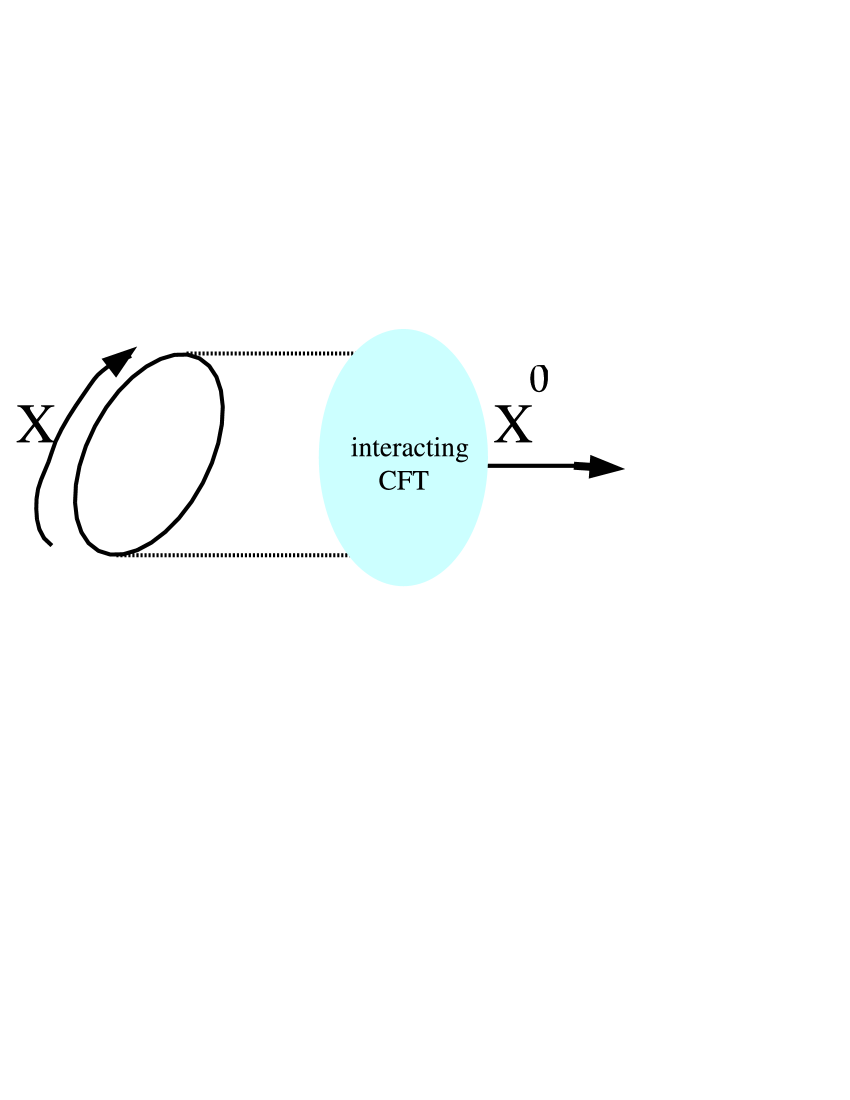
Figure 3: Behavior of the worldsheet theory: For large negative ${X^{0}{}}$, the worldsheet theory is a free CFT of $10+n$ embedding coordinates whose dilaton gradient has magnitude $Q=-{\sqrt{n}\over 2}$. at intermediate ${X^{0}{}}$ the worldsheet theory is a nontrivial interacting CFT. For large positive ${X^{0}{}}$ it is a free CFT of $9+n$ embedding coordinates whose dilaton gradient has magnitude $Q=-{\sqrt{n-1}\over 2}$. To order $n^{-{1\over 2}}$, explicit calculation of the renormalization of the dilaton gradient at ${X^{0}{}}\to\infty$ supports this picture. To make the figure as simple as possible, we have not indicated the orbifolding of the coordinate $X$.

The classical behavior of the 2D worldsheet theory motivated this interpretation of the $(0,1)$ super-sine-Liouville action [2]. The tachyon of the orbifolded type ${\rm HO}^{+({n})/}$ theory couples to the heterotic string worldsheet as a mass term for one (or more) of the coordinates transverse to the orbifold fixed locus. As the tachyon grows with target space time ${X^{0}{}}$, the mass term gets larger and pins the fundamental string to the origin of the coordinate which is being eliminated. As a result, the number of spacetime dimensions describing the string theory is reduced as ${X^{0}{}}\to+\infty$. In the limit ${X^{0}{}}=+\infty$ the worldsheet theory is again free; it describes strings propagating in $10+n-\Delta n$ spacetime dimensions with gauge group $SO(32+n-\Delta n)$.

When superstrings propagate in flat space in a number of dimensions other than ten, there must be a linear dilaton gradient which compensates the central charge. It is necessary for the self-consistency of our interpretation that when the number $n+10$ of spacetime dimensions changes, the magnitude of the dilaton gradient must change to compensate, so that the combination

$$\begin{array}[]{c}{3\over 2}n-6Q^{2}\end{array}$$ (6.180)

remains unchanged, and in particular stays equal to zero.

The dynamical readjustment of the dilaton gradient is the sole feature of the expected spacetime background which cannot be understood at the classical level on the worldsheet. Happily, we have found that the theory contains quantum effects which supply the necessary change in the dilaton gradient. Physical expectations for the change in the dilaton gradient agree quantitatively with explicit calculation in the limit $n\to\infty$.

It would be interesting to study the properties of our theory beyond the one-loop level, including a nonperturbative definition of the theory and a proof of conformal invariance. Liouville and sine-Liouville theories with various amounts of supersymmetry have been constructed and solved exactly via many different methods. (See, for instance, [9]-[17].) We anticipate that a further study of the dynamics of $(0,1)$-supersymmetric sine-Liouville theory will yield may interesting insights into dynamical dimension change in string theory.

Acknowledgements

The authors are indebted to many of their colleagues for helpful discussions, particularly J. Maldacena, L. Susskind, G. Giribét, J. M${{}^{\underline{\rm c}}}$Greevy, S. Kachru, A. Pakman, S. Shenker, and E. Silverstein. S.H. would like to thank the participants of the IAS theory group meetings for comments and questions which did much to motivate this research, and also the Stanford ITP and the Perimeter Institute for hospitality while this work was in progress. X.L. gratefully acknowledges the Prospects in Theoretical Physics program for hospitality during the course of this research. The work of S.H. was supported by DOE Grant DE-FG02-90ER40542.

Appendix

A Direct renormalization of the dilaton gradient

For purposes of computing ’extensive’ terms, we can ignore the finite volume and finite curvature, and just replace the covariant derivatives with partial derivatives again.

This calculation will do little other than check that we have chosen a correct, supersymmetric definition of the measure. Many things, including simple (independent) rescalings of bosons and fermions in the same multiplet at the classical level, can produce a nonsupersymmetric result for the one-loop potential. This can of course be cancelled by a local counterterm, but it is most convenient to take a definition of the measure which does not require this.

For the purpose of evaluating traces, we will make use of the identity

$${{\rm Tr}f(\hat{p})={{{V_{WS}}}\over{(2\pi)^{2}}}\int d^{2}p~{}f(p).}$$ (A.181)

A.1 Effective potential and effecitve linear dilaton

The effective action for a scalar field ${X^{0}{}}$ which is constant on a round worldsheet of radius $R_{WS}$ has two contributions: the first is a potential, which scales with two powers $R_{WS}^{2}$ of the worldsheet radius; the second contribution is an effecitve coupling $f({X^{0}{}}){\cal R}^{(2)}$ to the worldsheet Ricci scalar. This term is down by two powers of $R_{WS}$ relative to the potential term.

In order to extract the term subleading in $R_{WS}$ in which we are interested, we first focus on the leading, potential term. Due to worldsheet supersymmetry, the contributions to the effective potential term will vanish due to cancellation between boson and fermion loops.

To extract the effective potential from the effective action, set the scalar ${X^{0}{}}$ to a fixed constant value and divide by the volume $V_{WS}=4\pi R_{WS}^{2}$ of the worldsheet. The effective action is ${\hbar\over 2}$ times the logarithm of the bosonic determinant minus the logarithm of the fermionic determinant. We will evaluate each finite-volume loop diagram separately, beginning with the bosonic loop.

A.2 Determinants in finite volume

A.2.1 The bosonic contribution to the potential

Consider a background ${X^{0}{}}(\sigma)={X^{0}{}}_{({0})}$ independent of $\sigma$, and let $M\equiv\mu{\rm exp}\{b{X^{0}{}}\}=\mu{\rm exp}\{b{X^{0}{}}_{({0})}\}$. The bosonic determinant is

$${\sum_{n=0}^{\infty}(2n+1)~{}\ln\left({{M^{2}}\over{({\mu^{\prime}{}})^{2}}}+{{n^{2}+n}\over{R_{WS}^{2}({\mu^{\prime}{}})^{2}}}\right)}$$ (A.182)

We regulate the determinant, the result of which is that we multiply each log by

$${B\left({{n^{2}+n}\over{R_{WS}^{2}\Lambda^{2}}}\right)}$$ (A.183)

The regulated sum is

$${\sum_{n=0}^{\infty}(2n+1)~{}\ln\left({{M^{2}}\over{({\mu^{\prime}{}})^{2}}}+{{n^{2}+n}\over{R_{WS}^{2}({\mu^{\prime}{}})^{2}}}\right)\cdot B\left({{n^{2}+n}\over{R_{WS}^{2}\Lambda^{2}}}\right)}$$ (A.184)

To evaluate this, let us use the Euler-Maclaurin formula

$$\begin{array}[]{c}\sum_{n=a}^{b}f(n)=\int_{a}^{b}dn~{}f(n)+{1\over 2}(f(a)+f(b))+{1\over{12}}\left(f^{\prime}{}(b)-f^{\prime}{}(a)\right)+o(f^{\prime\prime\prime})\\ \\ =T_{-1}+T_{0}+T_{1}+{\rm remainder}\end{array}$$ (A.188)

$$\begin{array}[]{c}T_{-1}\equiv\int_{0}^{\infty}dn~{}(2n+1)~{}\ln\left({{M^{2}}\over{({\mu^{\prime}{}})^{2}}}+{{n^{2}+n}\over{R_{WS}^{2}({\mu^{\prime}{}})^{2}}}\right)\cdot B\left({{n^{2}+n}\over{R_{WS}^{2}\Lambda^{2}}}\right)\\ \\ =\Lambda^{2}R_{WS}^{2}\int_{0}^{\infty}du\left[~{}\ln\left({{\Lambda^{2}}\over{({\mu^{\prime}{}})^{2}}}\right)+\ln\left({{M^{2}}\over{\Lambda^{2}}}+u\right)\right]B(u)\end{array}$$ (A.192)

By taking $\Lambda^{2}{d\over{d\Lambda^{2}}}$ of the integral (without the $R^{2}\Lambda^{2}$ prefactor) we can see that the leading divergence is a potential of the form

$$\begin{array}[]{c}V(M)={\hbar\over 2}T_{-1}={\hbar\over{8\pi}}\left(I_{1}\Lambda^{2}\ln\left({{\Lambda^{2}}\over{({\mu^{\prime}{}})^{2}}}\right)+I_{2}\Lambda^{2}\right)\end{array}$$ (A.194)

where

$${I_{1}\equiv\int_{0}^{\infty}du~{}B(u),\hskip 36.135pt\hskip 36.135pt\hskip 36.135ptI_{2}\equiv\int_{0}^{\infty}du~{}B(u)~{}\ln u}$$ (A.195)

Note that this ’potential’ is actually a cosmological constant, having no dependence on $M$. It explicitly breaks scale invariance (since it is a term coming from the regulator) and must be subtracted off with a counterterm in order to restore scale invariance if it is not cancelled by another effect, which of course it is in the supersymmetric theory.

A.2.2 The fermionic contribution to the effective potential

Now let’s redo this for the fermionic determinant. In some basis, the operator ${\cal D}\equiv\Gamma^{i}\nabla_{i}$ is equal to [18]

$${{1\over R_{WS}}\left[\matrix{i(n+1)&0\cr 0&-i(n+1)}\right],}$$ (A.196)

with multiplicity $2n+2$.

So the eigenvalues of ${\cal D}+M$ are equal to $M\pm{{i(n+1)}\over R_{WS}},n\geq 0$, with multiplicity $2n+2$ each.

In order to take the regulator into account, we use the fact that $(\Gamma^{i}\nabla_{i})^{2}=\nabla^{i}\nabla_{i}-{1\over 4}{\cal R}^{(2)}$. This is the ’Weitzenbock formula’, but it is straighforward to work out by hand. For a spherical worldsheet of radius $R_{WS}$, the Ricci scalar is ${2\over{R_{WS}^{2}}}$, so

$${\nabla^{2}={\cal D}^{2}+{1\over{2R_{WS}^{2}}}={{{1\over 2}-(n+1)^{2}}\over{R_{WS}^{2}}}}$$ (A.197)

So the log of the regulated determinant is

$$\begin{array}[]{c}\sum_{n=0}^{\infty}~{}(2n+2)~{}\ln\left({{M^{2}}\over{({\mu^{\prime}{}})^{2}}}+{{(n+1)^{2}}\over{R_{WS}^{2}({\mu^{\prime}{}})^{2}}}\right)~{}B\left({{(n+1)^{2}-{1\over 2}}\over{R_{WS}^{2}\Lambda^{2}}}\right)\end{array}$$ (A.199)

A.2.3 The extensive term

First we extract the term $T_{-1}$ proportional to volume.

This term is

$$\begin{array}[]{c}T_{-1}\equiv\int_{0}^{\infty}dn~{}(2n+2)~{}\ln\left({{M^{2}}\over{({\mu^{\prime}{}})^{2}}}+{{(n+1)^{2}}\over{R_{WS}^{2}({\mu^{\prime}{}})^{2}}}\right)~{}B\left({{(n+1)^{2}-{1\over 2}}\over{R_{WS}^{2}\Lambda^{2}}}\right)\\ \\ =\Lambda^{2}R_{WS}^{2}\int_{0}^{\infty}du~{}\left\{\ln\left({{\Lambda^{2}}\over{({\mu^{\prime}{}})^{2}}}\right)+\ln\left({{M^{2}}\over{\Lambda^{2}}}+{1\over{R_{WS}^{2}\Lambda^{2}}}+u\right)\right\}~{}B\left(u+{{1}\over{2R_{WS}^{2}\Lambda^{2}}}\right)\\ \\ \end{array}$$ (A.202)

where we have used the changes of variables $t\equiv(n+1)^{2}-{1\over 2}$ and $u\equiv{t\over{\Lambda^{2}R_{WS}^{2}}}$.

To leading order in $R_{WS}^{2}\Lambda^{2}$, the integrand is the same as in the log of the bosonic determinant. The difference is of subleading order in $R_{WS}^{2}\Lambda^{2}$ and it is equal to

$$\begin{array}[]{c}T_{-1}^{fermionic}-T_{-1}^{bosonic}{}{}{}\\ \\ \simeq\Lambda^{2}R_{WS}^{2}\int_{0}^{\infty}du~{}{1\over{\Lambda^{2}R_{WS}^{2}}}{1\over{{{M^{2}}\over{\Lambda^{2}}}+u}}B(u)+\ln\left({{M^{2}}\over{\Lambda^{2}}}+u\right){1\over{2\Lambda^{2}R_{WS}^{2}}}B^{\prime}{}(u)~{}~{}~{},\end{array}$$ (A.205)

with a remainder which vanishes as $\Lambda^{2}\to\infty$ with the other quantities held fixed. The first term in the integrand was obtained by expanding the logarithm in ${1\over{\Lambda^{2}R_{WS}^{2}}}$, the second term by expanding the regulator function in ${1\over{\Lambda^{2}R_{WS}^{2}}}$.

First, we point out that in the limit $\Lambda^{2}R_{WS}^{2}\to\infty$, the second term asymptotes to a constant, and does not behave as a logarithm of $M$. This is useful to us, as it means that the renormalization of the dilaton gradient will not depend on the form of the regulator function, in accordance with the field-theoretic principle of universality.

The second term is equal to $f({{M^{2}}\over{\Lambda^{2}}})$, where

$$\begin{array}[]{c}f(x)\equiv\int_{0}^{\infty}du~{}B^{\prime}{}(u)\ln\left(x+u\right)\\ \\ \end{array}$$ (A.208)

We are interested in the coefficient of $\ln x$ in the expansion of $f(x)$ as $x\to 0$. To extract this coefficient, we can differentiate under the integral sign:

$$\begin{array}[]{c}{{d~{}f(x)}\over{d~{}\ln x}}=xf^{\prime}{}(x)\\ \\ =\int_{0}^{\infty}{{B^{\prime}{}(u)~{}x~{}du}\over{u+x}}\\ \\ =\left.{{x~{}B(u)}\over{x+u}}\right|_{0}^{\infty}+\int_{0}^{\infty}~{}{{B(u)~{}x~{}du}\over{(u+x)^{2}}}\\ \\ =-1+\int_{0}^{\infty}{{B(xv)~{}dv}\over{(v+1)^{2}}}\end{array}$$ (A.216)

In the limit $x\to 0$ the function $B(xv)$ approaches $1$ for any finite $v$, so we have

$${-1+\int_{0}^{\infty}{{dv}\over{(v+1)^{2}}}=0}$$ (A.217)

In fact, it is easy to check that the limit $\Lambda\to\infty$ is finite, and given by the integral

$$\begin{array}[]{c}I_{3}\equiv\int_{0}^{\infty}~{}B^{\prime}{}(u)~{}du~{}\ln u,\end{array}$$ (A.219)

giving a finite renormalization of the cosmological constant which can be removed with a counterterm.

So we are left with

$$\begin{array}[]{c}\int_{0}^{\infty}~{}{{B(u)du}\over{x+u}},\end{array}$$ (A.221)

with $x={{M^{2}}\over{\Lambda^{2}}},$ as before. Again, taking $x{d\over{dx}}$ of this quantity and taking $x\to 0$, we get

$$\begin{array}[]{c}-\int_{0}^{\infty}{1\over{(v+1)^{2}}}=-1\end{array}$$ (A.223)

So the total $T_{-1}$ contribution of the $X,{\tilde{\lambda}},\psi^{X}{}$ degrees of freedom to the effective action

$$\begin{array}[]{c}-{\hbar\over 2}\left[I_{3}+I_{4}-\ln\left({{M^{2}}\over{\Lambda^{2}}}\right)\right],\end{array}$$ (A.225)

where

$${I_{4}\equiv\int_{0}^{\infty}{{B(u)~{}du}\over{u+1}}}$$ (A.226)

in the limit $\Lambda\to\infty$.

There are still nonzero contributions at the $T_{0}$ and $T_{1}$ terms, but these are finite and so are easier to evaluate.

A.3 Bosonic and fermionic $T_{0}$ and $T_{1}$ contributions

There are also contributions to the effective dilaton coupling from subleading terms in the Euler-Maclaurin expansion. We now evaluate the $T_{0}$ and $T_{1}$ contributions.

A.3.1 Bosonic $T_{0}$ contribution

Since $B(u)$ vanishes with all its derivatives at $u\to\infty$, so $T_{0}$ contribution to the logarithm of the bosonic determinant is

$$\begin{array}[]{c}{1\over 2}\left.\left[(2n+1)\ln\left({{M^{2}}\over{({\mu^{\prime}{}})^{2}}}+{{n^{2}+n}\over{R_{WS}^{2}({\mu^{\prime}{}})^{2}}}\right)\cdot B\left({{n^{2}+n}\over{R_{WS}^{2}\Lambda^{2}}}\right)\right]\right|_{n=0}={1\over 2}\ln\left({{M^{2}}\over{({\mu^{\prime}{}})^{2}}}\right)\end{array}$$ (A.228)

$T_{0}$ and higher terms are automatically ultraviolet finite, so $\Lambda$ cannot enter them. Also, they will depend on the regulator only through its derivatives at the origin. $T_{0}$ contributions, in particular, are independent of the regulator function altogether.

A.3.2 Fermionic $T_{0}$ contribution

The

$$\begin{array}[]{c}{1\over 2}\left.\left[~{}(2n+2)~{}\ln\left({{M^{2}}\over{({\mu^{\prime}{}})^{2}}}+{{(n+1)^{2}}\over{R_{WS}^{2}({\mu^{\prime}{}})^{2}}}\right)~{}B\left({{(n+1)^{2}-{1\over 2}}\over{R_{WS}^{2}\Lambda^{2}}}\right)\right]\right|_{n=0}\\ \\ =1\cdot\ln\left({{M^{2}}\over{({\mu^{\prime}{}})^{2}}}\right)+o\left({1\over{R_{WS}^{2}}}\right)\end{array}$$ (A.232)

A.3.3 Bosonic and fermionic $T_{1}$ contributions

These contributions come by differentiating the expression for the $n^{\rm{\underline{th}}}$ term by $n$ and evaluating at zero. Up to terms of order $R_{WS}^{-2}$, both bosonic and fermionic summands have the same $n$-derivative at zero, namely

$${2\ln\left({{M^{2}}\over{({\mu^{\prime}{}})^{2}}}\right).}$$ (A.233)

Since bosonic and fermionic determinants contribute oppositely to the effective action, these two contributions cancel.

A.3.4 Summing up the effective dilaton contributions

The contributions to the effective action are as follows:

$$\begin{array}[]{c}{\hbar\over 2}\left[\ln\left({{M^{2}}\over{\Lambda^{2}}}\right)-I_{3}-I_{4}+{1\over 2}\ln\left({{M^{2}}\over{({\mu^{\prime}{}})^{2}}}\right)-\ln\left({{M^{2}}\over{({\mu^{\prime}{}})^{2}}}\right)\right]=\left({\rm terms~{}which~{}vanish~{}as~{}}\Lambda\to\infty\right)\end{array}$$

So as the regulator is removed and setting $\hbar=1$, we are left with

$$\begin{array}[]{c}={1\over 4}\ln\left({{M^{2}}\over{\mu^{2}}}\right)+\left(M-{\rm independent}\right).\end{array}$$ (A.236)

So, the effective action on the sphere is enhanced by a factor of ${1\over 2}bX^{0}+\left(X^{0}-{\rm independent}\right)$, which we interpret as being equal to $+2\Delta_{\rm one-point}\Phi$, since we are working on the sphere. The notation is intended to convey the idea that this renormalization comes from the renormalized one-point function for $X^{0}$ (extracting the subleading term in volume on a finite-sized sphere).

B Wavefunction renormalization of $X^{0}$

There is another contribution to the dilaton coupling renormalization which comes from the renormalization of the two-point function for $X^{0}$, which we shall call $\Delta_{\rm two-point}\Phi$.

The origin of this term is as follows. One effect of integrating out the $X,{\tilde{\lambda}},\psi^{X}{}$ degrees of freedom is that $X^{0}$ receives a wavefunction renormalization, which as we shall see is proportional to $b^{2}$. Let us say the (Euclidean) kinetic term receives an effective contribution ${1\over{4\pi}}(c_{1}b^{2})(\vec{\partial}{X^{0}{}})^{2}$, where $c_{1}$ is some numerical constant which will be calculated from a loop diagram. Then in order to re-canonicalize the field ${X^{0}{}}$ at large ${X^{0}{}}$ we must rescale ${X^{0}{}}$ by a factor $(1+c_{1}b^{2})^{-{1\over 2}}\sim 1-{1\over 2}c_{1}b^{2}+o(b^{4})$. As a result, the ${Q^{E}}X^{0}{\cal R}$ term in the original bare lagrangian gets scaled by that factor and the result is a term equal to

$$\begin{array}[]{c}-{1\over 2}c_{1}b^{2}{Q^{E}}\cdot{1\over{4\pi}}\int{d^{2}\sigma}~{}\sqrt{g}~{}{\cal R}^{({2})}{\tilde{{X^{0}{}}}},\end{array}$$ (B.238)

where $\tilde{{X^{0}{}}}$ is the field ${X^{0}{}}$, rescaled so that its loop-corrected effective kinetic term has canonical normalization.

In the small-b branch of the large-n limit, the original dilaton gradient ${Q^{E}}$ is of order $n^{+{1\over 2}}$ and $b$ is of order $n^{-{1\over 2}}$. So the ’two-point’ renormalization $\delta{Q^{E}}=-{1\over 2}c_{2}b^{2}{Q^{E}}$ is of order $n^{-{1\over 2}}$, just like the ’one-point’ contribution $\delta{Q^{E}}={1\over 4}b$. We must take this effect into account as well.

In the following section, we will not bother to make the volume finite, since the term we are interested in scales as $R_{WS}^{2}$; it is an extensive term.

B.1 Effective kinetic term from effective action

The effective action coming from the loop of massive particles we can calculate in terms of logarithms of determinants. In this subsection we will write the expression for the effective kinetic term in terms of the effective action.

If our effective action is of the form

$${{\cal S}=\int~{}d^{2}\sigma~{}\kappa~{}(\vec{\partial}{X^{0}{}})^{2},}$$ (B.239)

then we can extract $\kappa$ by setting

$${{X^{0}{}}\equiv w+\epsilon~{}{\rm exp}\{ik\sigma\}+\epsilon^{*}{\rm exp}\{-ik\sigma\},}$$ (B.240)

where $w$ is the constant background value of ${X^{0}{}}$, and taking derivatives of the action with respect to $k$ and $\epsilon^{({1,2})}$. Plug in this value for ${X^{0}{}}$ and the action is

$$\begin{array}[]{c}\kappa\left[(\epsilon\cdot i\vec{k})(\epsilon^{*}\cdot(-i\vec{k}))\cdot 2\right]\left[V_{WS}\right]\\ \\ =2\kappa~{}V_{WS}\epsilon\epsilon^{*}{\vec{k}}^{2},\end{array}$$ (B.244)

where $V_{WS}$ is the volume of the worldsheet $\int d^{2}\sigma$.

Take ${\delta\over{\epsilon}}{\delta\over{\epsilon^{*}}}$ of this and get $2\kappa V_{WS}\vec{k}^{2}$.

Take ${1\over 2}{\delta\over{\delta k^{2}}}={1\over 8}{\delta\over{\delta k^{a}}}{\delta\over{\delta k_{a}}}$ of this and get $\kappa~{}{V_{WS}}$. So

$$\begin{array}[]{c}\kappa=\left.{1\over{8~{}{V_{WS}}}}{\delta\over{\delta k^{a}}}{\delta\over{\delta k_{a}}}{\delta\over{\delta\epsilon}}{\delta\over{\delta\epsilon^{*}}}{\cal S}\left[w+\epsilon~{}{\rm exp}\{ik\sigma\}+\epsilon^{*}{\rm exp}\{-ik\sigma\}\right]\right|_{\epsilon=k=0}\\ \\ =\left.{1\over{2~{}{V_{WS}}}}{\delta\over{\delta k^{2}}}{\delta\over{\delta\epsilon}}{\delta\over{\delta\epsilon^{*}}}{\cal S}\left[w+\epsilon~{}{\rm exp}\{ik\sigma\}+\epsilon^{*}{\rm exp}\{-ik\sigma\}\right]\right|_{\epsilon=k=0}\end{array}$$

So now let us evaluate the bosonic and fermionic determinants, evaluated with the background value

$${{X^{0}{}}=w+\epsilon~{}{\rm exp}\{ik\sigma\}+\epsilon^{*}{\rm exp}\{-ik\sigma\}}$$ (B.248)

Since we are aiming to extract only the ’extensive’ contribution, we will take only the $T_{-1}$ term, and the volume of the worldsheet will enter only through the formula

$${{\rm Tr}~{}f(-i\partial_{a})={{V_{WS}}\over{(2\pi)^{2}}}\int d^{2}p~{}f(p_{a})}$$ (B.249)

B.2 Bosonic contribution

Defining $M(\sigma)\equiv\mu~{}{\rm exp}\{b{X^{0}{}}(\sigma)\}$ and $M_{({0})}\equiv\mu~{}{\rm exp}\{b{X^{0}{}}_{({0})}\}$, the log of the bosonic determinant is

$$\begin{array}[]{c}{\rm Tr}~{}\ln~{}\left[{1\over{({\mu^{\prime}{}})^{2}}}\left((-i\partial)^{2}+M(\sigma)^{2}\right)\right]\\ \\ ={\rm Tr}~{}\ln~{}\left[{1\over{({\mu^{\prime}{}})^{2}}}\left((-i\partial)^{2}+M^{2}\right)\right]+{\rm Tr}~{}\left[\left((-i\partial)^{2}+M^{2}\right)^{-1}~{}\delta M^{2}(\sigma)\right]\\ \\ -{1\over 2}{\rm Tr}~{}\left[\left((-i\partial)^{2}+M^{2}\right)^{-1}~{}\delta M^{2}(\sigma)~{}\left((-i\partial)^{2}+M^{2}\right)^{-1}~{}\delta M^{2}(\sigma)\right]+o\left(\delta M^{2}(\sigma)\right)^{3}\end{array}$$ (B.255)

Only the term of order $o\left(\delta M^{2}(\sigma)\right)^{2}$ will give a nonvanishing $\epsilon\epsilon^{*}$ piece. Using $\delta M^{2}=2bM^{2}\delta{X^{0}{}}$, we find this piece is equal to

$$\begin{array}[]{c}-4b^{2}M^{4}~{}\epsilon\epsilon^{*}~{}{\rm Tr}~{}\left[\left((-i\partial)^{2}+M^{2}\right)^{-1}~{}{\rm exp}\{ik\sigma\}~{}\left((-i\partial)^{2}+M^{2}\right)^{-1}~{}{\rm exp}\{-ik\sigma\}\right]\\ \\ =-4b^{2}M^{4}\epsilon\epsilon^{*}~{}{\rm Tr}~{}\left[\left((-i\partial+k)^{2}+M^{2}\right)^{-1}\left((-i\partial)^{2}+M^{2}\right)^{-1}\right]\\ \\ =-{{4b^{2}M^{4}\epsilon\epsilon^{*}V_{WS}}\over{4\pi^{2}}}\int d^{2}p~{}\left[\left((p+k)^{2}+M^{2}\right)^{-1}\left(p^{2}+M^{2}\right)^{-1}\right]\end{array}$$ (B.261)

We are only interested in the piece which is quadratic in $k$, which is

$$\begin{array}[]{c}-{{4b^{2}M^{4}\epsilon\epsilon^{*}V_{WS}}\over{4\pi^{2}}}\int d^{2}p~{}\left[{{-k^{2}}\over{(p^{2}+M^{2})^{3}}}+{{4k_{a}k_{b}p^{a}p^{b}}\over{(p^{2}+M^{2})^{4}}}\right]\\ \\ =+{1\over{6\pi}}\cdot b^{2}\cdot V_{WS}\cdot\epsilon\epsilon^{*}k^{2}\end{array}$$ (B.265)

To get the corresponding contribution to the effective action, multiply by $+{\hbar\over 2}$, to get

$${\Delta{\cal S}_{{\rm bos.}}=+{{1}\over{12\pi}}\cdot\hbar\cdot b^{2}\cdot V_{WS}\cdot\epsilon\epsilon^{*}k^{2}.}$$ (B.266)

B.3 Fermionic contribution

The fermionic calculation is similar. The determinant is

$$\begin{array}[]{c}{\rm Tr}~{}\ln~{}\left[{\cal D}(M+\delta M)\right],\end{array}$$ (B.268)

where ${\cal D}\equiv\left[\Gamma^{i}(-i\partial_{i})+iM(\sigma)\right]=\left[({\hat{p}}\cdot\Gamma)+iM(\sigma)\right]$. This operator is not Hermitean, but its determinant is real.

For constant $M$, its inverse

$${\hat{\Delta}({\hat{p}},M)={\cal D}^{-1}({\hat{p}},M)\equiv({\hat{p}}^{2}+M^{2})^{-1}(({\hat{p}}\cdot\Gamma)-iM)}$$ (B.269)

defines the propagator.

The piece of the log of the determinant with two fluctuations is

$$\begin{array}[]{c}=-{1\over 2}~{}{\rm Tr}~{}\left[\hat{\Delta}({\hat{p}},M)\cdot(-i\delta M)\cdot\hat{\Delta}({\hat{p}},M)\cdot(-i\delta M)\right]\\ \\ =+b^{2}M_{({0})}^{2}|\epsilon|^{2}~{}{\rm Tr}~{}\left[\hat{\Delta}({\hat{p}},M)\cdot{\rm exp}\{ik\sigma\}\cdot\hat{\Delta}({\hat{p}},M)\cdot{\rm exp}\{-ik\sigma\}\right]\\ \\ =b^{2}M_{({0})}^{2}|\epsilon|^{2}~{}{\rm Tr}~{}\left[\hat{\Delta}({\hat{p}}+k,M)\cdot\hat{\Delta}({\hat{p}},M)\right]\\ \\ =b^{2}M_{({0})}^{2}|\epsilon|^{2}{{V_{WS}}\over{4\pi^{2}}}\cdot\int d^{2}p~{}{\rm tr}\left[\hat{\Delta}(p+k,M)\cdot\hat{\Delta}(p,M)\right]\\ \\ =+2(b~{}M~{}\epsilon)(b~{}M~{}\epsilon^{*})\cdot{1\over 2}\cdot{{V_{WS}}\over{4\pi^{2}}}\cdot I(k^{2}),\end{array}$$

where

$$\begin{array}[]{c}I(k^{2})\equiv\int d^{2}p~{}{\rm tr}\left[\left(\Gamma\cdot(p+k)+iM\right)^{-1}\cdot\left(\Gamma\cdot p+iM\right)^{-1}\right]\end{array}$$ (B.280)

We wish to extract the order $k^{2}$ piece $I^{\prime}{}(0)=\left.I^{\prime}{}(k^{2})\right|_{k=0}=\left.{1\over 4}{\delta\over{\delta k^{a}}}{\delta\over{\delta k_{a}}}~{}I(k^{2})\right|_{k=0}$ of the amplitude $I(k^{2})$. Differentiating under the integral sign, we get

$$\begin{array}[]{c}{\delta\over{\delta k^{a}}}I(k^{2})=-\int d^{2}p~{}{\rm tr}\left[\hat{\Delta}(p+k,M)\Gamma^{a}\hat{\Delta}(p+k,M)\hat{\Delta}(p,M)\right]\\ \end{array}$$

and

$$\begin{array}[]{c}{\delta\over{\delta k^{a}}}{\delta\over{\delta k_{a}}}I(k^{2})=+2\int d^{2}p~{}{\rm tr}\left[\hat{\Delta}(p+k,M)\Gamma_{a}\hat{\Delta}(p+k,M)\Gamma^{a}\hat{\Delta}(p+k,M)\hat{\Delta}(p,M)\right]\end{array}$$

so

$$\begin{array}[]{c}I^{\prime}{}(0)=\left.{1\over 4}{\delta\over{\delta k^{a}}}{\delta\over{\delta k_{a}}}I(k^{2})\right|_{k=0}\\ \\ ={1\over 2}\int d^{2}p~{}{\rm tr}~{}\left[\hat{\Delta}^{3}(p,M)\Gamma^{a}\hat{\Delta}(p,M)\Gamma_{a}\right]\end{array}$$ (B.285)

Using the fact that

$$\begin{array}[]{c}{\rm tr}\left[\hat{\Delta}^{3}(p,M)\Gamma^{a}\hat{\Delta}(p,M)\Gamma_{a}\right]=4M^{2}{{M^{2}-3p^{2}}\over{(p^{2}+M^{2})^{4}}}\end{array}$$ (B.287)

and we conclude that

$$\begin{array}[]{c}I^{\prime}{}(0)={1\over 2}\cdot 4M^{2}\int~{}d^{2}p~{}{{M^{2}-3p^{2}}\over{(p^{2}+M^{2})^{4}}}\end{array}$$

and

$$\begin{array}[]{c}\left.\ln~{}{\rm Det}(A)\right|_{o(\epsilon{}^{*}\epsilon~{}k^{2})}=-{1\over{12\pi}}b^{2}{V_{WS}}\epsilon\epsilon^{*}k^{2}.\end{array}$$ (B.290)

To get the corresponding contribution to the action, multiply by $-{\hbar\over 2}$, to get

$$\begin{array}[]{c}\Delta{\cal S}_{\rm ferm.}=+{\hbar\over{24\pi}}b^{2}{V_{WS}}\epsilon\epsilon^{*}k^{2}.\end{array}$$ (B.292)

References

• [1]
• [2] S. Hellerman, “On the Landscape of Superstring Theory in D $>$ 10,” arXiv:hep-th/0405041.
• [3] A. Strominger and T. Takayanagi, “Correlators in timelike bulk Liouville theory,” Adv. Theor. Math. Phys.  7, 369 (2003) [arXiv:hep-th/0303221].
• [4] S. P. de Alwis, J. Polchinski and R. Schimmrigk, “Heterotic Strings With Tree Level Cosmological Constant,” Phys. Lett. B 218, 449 (1989).
• [5] A. H. Chamseddine, “A Study of noncritical strings in arbitrary dimensions,” Nucl. Phys. B 368, 98 (1992).
• [6] J. Polchinski, “String Theory. Vol. 2: Superstring Theory And Beyond,”  (Cambridge University Press, 1998); correction to eq. (12.1.34b) at http://theory.itp.ucsb.edu/ joep/errata.html#c12.
• [7] S. Sugimoto, “Anomaly cancellations in type I D9-D9-bar system and the USp(32) string Prog. Theor. Phys.  102, 685 (1999) [arXiv:hep-th/9905159] ;  J. H. Schwarz and E. Witten, JHEP 0103, 032 (2001) [arXiv:hep-th/0103099].
• [8] R. C. Myers, “New Dimensions For Old Strings,” Phys. Lett. B 199, 371 (1987).
• [9] T. L. Curtright and C. B. Thorn, Phys. Rev. Lett.  48, 1309 (1982) [Erratum-ibid.  48, 1768 (1982)].
• [10] T. Fukuda and K. Hosomichi, “Three-point functions in sine-Liouville theory,” JHEP 0109, 003 (2001) [arXiv:hep-th/0105217].
• [11] N. Seiberg, “Notes On Quantum Liouville Theory And Quantum Gravity,” Prog. Theor. Phys. Suppl.  102, 319 (1990).
• [12] A. M. Polyakov, Phys. Lett. B 103, 211 (1981).
• [13] E. D’Hoker, Phys. Rev. D 28, 1346 (1983).
• [14] D. Kutasov and N. Seiberg, Phys. Lett. B 251, 67 (1990).
• [15] H. Dorn and H. J. Otto, Nucl. Phys. B 429, 375 (1994) [arXiv:hep-th/9403141].
• [16] M. Goulian and M. Li, “Correlation Functions In Liouville Theory,” Phys. Rev. Lett.  66, 2051 (1991).
• [17] J. Teschner, Phys. Lett. B 363, 65 (1995) [arXiv:hep-th/9507109].
• [18] R. Camporesi and A. Higuchi, “On the Eigen functions of the Dirac operator on spheres and real hyperbolic spaces,” arXiv:gr-qc/9505009.