hep-th/0409069

UT-04-23 September, 2004

Cardy states, factorization and
idempotency in closed string field theory

Isao Kishimoto and Yutaka Matsuo

Department of Physics, Faculty of Science, University of Tokyo
Hongo 7-3-1, Bunkyo-ku, Tokyo 113-0033, Japan

We show that boundary states in the generic on-shell background satisfy a universal nonlinear equation of closed string field theory. It generalizes our previous claim for the flat background. The origin of the equation is factorization relation of boundary conformal field theory which is always true as an axiom. The equation necessarily incorporates the information of open string sector through a regularization, which implies the equivalence with Cardy condition. We also give a more direct proof by oscillator representations for some nontrivial backgrounds (torus and orbifolds). Finally we discuss some properties of the closed string star product for non-vanishing $B$ field and find that a commutative and non-associative product (Strachan product) appears naturally in Seiberg-Witten limit.

1 Introduction

Since its discovery, D-brane has been one of the central objects of interest in string theory. It represents fundamental nonperturbative features and is an analog of the soliton excitation in string theory.

In conformal field theory, the D-brane is described by boundary state. It belongs to the closed string Hilbert space and is implemented by the boundary conditions such as,

$$\partial_{\tau}X^{\mu}|_{\tau=0}|B\rangle_{\mathrm{Neumann}}=0\,,\quad\mbox{or }\quad\partial_{\sigma}X^{\mu}|_{\tau=0}|B\rangle_{\mathrm{Dirichlet}}=0\,.$$ (1.1)

These equations determine the state $|B\rangle$ up to normalization constant. The information of the open strings which live on D-brane can be extracted from $|B\rangle$ after modular transformation,

$$\langle B|q^{{1\over 2}\left(L_{0}+\tilde{L}_{0}-\frac{c}{12}\right)}|B\rangle=\mbox{Tr}_{\mathcal{H}_{\mathrm{open}}}\tilde{q}^{L_{0}-\frac{c}{24}}\,,\quad\tilde{q}\equiv e^{4\pi^{2}/\log q}\,.$$ (1.2)

For more generic (conformal invariant) background where we can not use the free field oscillators as above, the boundary condition can be implemented only through generators of Virasoro algebra,

$$(L_{n}-\tilde{L}_{-n})|B\rangle=0\,.$$ (1.3)

This condition is universal in a sense that it does not depend on a particular representation of Virasoro algebra which corresponds to the background.

This linear equation, however, is not enough to characterize the D-brane completely. We need further constraints that the open string sectors derived from them should be well-defined. More explicitly, take two states $|B_{i}\rangle$ ($i=1,2$) which satisfy eq. (1.3). The open string sector appears in the annulus amplitude after the modular transformation can be written as,

$$\chi_{12}(q)=\langle B_{1}|q^{{1\over 2}\left(L_{0}+\tilde{L}_{0}-\frac{c}{12}\right)}|B_{2}\rangle=\sum_{i}\mathcal{N}_{12}^{i}\,\chi_{i}(\tilde{q})\,,\quad$$ (1.4)

where $\chi_{i}$ are characters of the irreducible representations in the open string channel. In order to have well-defined open string sector, the coefficients $\mathcal{N}_{12}^{i}$ must be non-negative integers. This is called Cardy condition [1]. We note that these are non-linear (quadratic) constraints in terms of the boundary states.

These conditions (1.3, 1.4) are written in terms of the boundary conformal field theory. In this sense, it is at the level of the first quantization. In order to consider the off-shell process, such as tachyon condensation, we need to use the second quantized description. One of the strong candidates of the off-shell descriptions of string theory is string field theory. Therefore, it is natural to ask whether one may derive conditions which are equivalent to (1.3, 1.4) in that language.

There are a few species of string field theories. The best-established one is Witten’s open bosonic string field theory [2]. In terms of this formulation, the annihilation process of unstable D-branes was first studied extensively and it established the idea of “tachyon vacuum” by computation of the D-brane tension numerically [3].

In this paper, however, we do not use this formulation since the dynamical variables of open string field theory depend essentially on the D-brane where the open string is attached. Since our goal is to find the characterization of generic consistent boundaries, this variable is not particularly natural because of this particular reference to the specific D-brane.

Since the boundary state belongs to the closed string Hilbert space, we will instead take the closed string field theory as the basic language. With closed string variable, the description of the linear constraint (1.3) is trivial: $(L_{n}-\tilde{L}_{-n})\Phi=0$. On the other hand, the description of the Cardy condition (1.4) is much more nontrivial since it is the requirement to the open string channel which appears only after the modular transformation. Furthermore, it is a nonlinear relation. If it is possible to represent it in string field theory, one needs to use the closed string star product to express nonlinear relations.

There are two types of closed string star products which have been studied in the literature. The first one is Zwiebach’s star product which is a closed string version of Witten’s open string star product [4, 5] and the other one is a covariant version of the light-cone string field theory (HIKKO’s vertex) [6]. They are defined through the overlap of three strings as depicted in Fig. 1.

Figure 1: Closed string vertices

These vertices are constructed to define the closed string field theories proposed by these authors. In this paper, however, our main focus is the algebraic structure between boundary states. Indeed, the nonlinear relation which we are going to study holds for both of these two vertices. In a sense, our relation does not seem to be a consequence of their proposed action at least at this moment but rather comes directly from the basic properties of the boundary conformal field theory.

The nonlinear equation has been proposed and studied in our previous papers [7, 8, 9]. It can be written as an idempotency relation among boundary states,

$$\Phi\star\Phi=\mathcal{C}\,T_{B}^{-1}c_{0}^{+}\Phi,\quad(\Phi\equiv c_{0}^{-}b_{0}^{+}|B\rangle\,,\,T_{B}\equiv\langle 0|c_{-1}\tilde{c}_{-1}c_{0}^{-}|B\rangle)\,,$$ (1.6)

where $T_{B}$ is the tension of the D-brane associated with the boundary state $|B\rangle$. In the first paper [7], we proved it for the usual D$p$-brane boundary states for $\Phi$ and HIKKO vertex for $\star$. A surprise was that this equation is universal for any boundary states which we considered including the coefficient $\mathcal{C}$ [8]. The proof is based on an explicit calculation with the oscillator representation [6]. In the second paper [8], we gave an outline of the proof of the same equation for Zwiebach’s vertex. The equation takes the same form for these two vertices except for the overall constant $\mathcal{C}$. From these observations, we conjectured that eq. (1.6) is a background independent characterization of the boundary state.

Toward that direction, in [8], we used the path integral definition of the string field theory in terms of the conformal mapping [14] and tried to prove the relation in the general background. After some efforts, we have arrived at a weaker statement: suppose $|B_{i}\rangle$ ($i=1,2$) satisfy the linear constraint (1.3), the state $|B_{1}\rangle\star|B_{2}\rangle$ also satisfies the same constraint. It proves that product of any boundary state in weak sense becomes again boundary state in weak sense. This does not, of course, imply the Cardy constraint (1.4) and, in particular, we could not understand the role of the open string sector.

One of the purposes of this paper is to discuss the link with open string which was missed in our previous studies and establish more explicit relation between (1.6) and the Cardy condition. A crucial hint to this problem is that the coefficient $\mathcal{C}$ in the relation (1.6) is actually divergent and it is necessary to introduce some sort of regularization in the computation. In [7], we cut-off the rank of Neumann coefficient by $K$. Then the divergent coefficient behaves as $\mathcal{C}\sim K^{3}$. In LPP approach, on the other hand, another type of the regularization can be introduced by slightly shifting the interaction point on the world sheet. Such a shift gives a small strip which interpolates between two holes associated with the boundary. In the limit of turning-off the regulator, the moduli parameter which describes the shape of the strip becomes zero. This is the usual factorization process where the world sheet becomes degenerate [15]. An essential point is that such a factorization process occurs in the open string channel between the two holes. In this way, the equation for the string field (1.6) can be related with the consistency of the dual open string channel. The leading singularity comes from the propagation of the open string tachyon which is universal for any boundary states in arbitrary background and it explains our claim that the divergent factor $\mathcal{C}$ is also universal for any Cardy states.

This outline will be explained in detail in section 2. We will also repeat our previous discussion [8] that only the boundary states can satisfy the equation (1.3). By combining these ideas, it will be obvious that the nonlinear equation (1.3) plays an essential rôle to understand D-branes in the context of string field theory.

At this point, it may be worth while to mention that our claims are remarkably similar to the scenario conjectured in vacuum string field theory [16]. The form of the equation is exactly the same except that the dynamical variables and the star product are totally different. There is no nontrivial solution in the vicinity of $\Phi=0$ and the non-vanishing solutions correspond to D-branes. In a sense, our equation is an explicit realization of VSFT scenario in the dual closed string channel. While the dynamical variables is closed string field, the physical excitations around the boundary state are on-shell open string mode [7, 8].

Our discussion in section 2 is based on the path integral and the argument becomes necessarily formal to some extent. In this sense, it is desirable to check the consistency of the argument in the oscillator representation for some non-trivial backgrounds. Fortunately, there are explicit forms of the three string vertex for (1) toroidal $T^{d}$ and (2) orbifold $T^{d}/Z_{2}$ compactification [17, 18].

In both cases, the three string vertex has some modifications compared to that on the flat background ${\bf R}^{d}$ [6]. One needs to include cocycle factor due to the existence of winding mode and take into account the twisted sector in orbifold case. The cocycle factor is needed to keep Jacobi identity for the $\star$ product of the closed string field theory. In section 3, we perform explicit computation of $\star$ product among the boundary (Ishibashi) states. For torus case, there appear extra cocycle factors in the algebra of Ishibashi states and some care is needed to construct Cardy states as idempotents of the algebra. For the orbifold case, mixing between untwisted sector and twisted sector is needed to describe the fractional D-branes. The ratio of the coefficients of the two sectors is given as the ratio of the determinants of the Neumann matrices for the (un)twisted sectors. We use various regularization methods to calculate them explicitly. This result is consistent with our previous arguments [9].

Finally, the third issue which will be discussed in section 4 is to incorpolate the noncommutativity on the D-brane. We have already seen in [7] that non-commutativity on the world volume of the D-brane forces us to use the open string metric to write down the on-shell conditions. This is possible since the explicit form of the boundary state is known for such cases. On the other hand, for the noncommutativity in the transverse directions, it is difficult to express in the language of the boundary conformal field theory. This is, however, an important set-up for matrix models or noncommutative Yang-Mills theory.

A motivation toward this direction is our previous study [8] where we have seen that an analog of the noncommutative soliton arises in the commutative limit. We note that the idempotency relation for the D$p$-brane takes the following form in the matter sector,

$$|B,x^{\perp}\rangle\star|B,y^{\perp}\rangle=\mathcal{C}_{d}\,\delta^{d-p-1}(x^{\perp}-y^{\perp})\,|B,y^{\perp}\rangle\,\,,$$ (1.7)

where $x^{\perp},\,y^{\perp}$ are the coordinates in the transverse directions. In order to recover the universal relation (1.6), we need to take a linear combination,

$$|B\rangle_{f}\equiv\int d^{d-p-1}x^{\perp}\,f(x^{\perp})|B,x^{\perp}\rangle\,\,.$$ (1.8)

Eq. (1.6) then implies $f^{2}(x^{\perp})=f(x^{\perp})$ which is the same as (1.5) in the commutative limit. It is, therefore, tempting to study what kind of modification will be necessary in the presence of $B$ field.

In order to study it, we consider a particular deformation of Ishibashi states which seems to be relevant to describe the noncommutativity along the transverse directions. We take the star product between them and take Seiberg-Witten limit. The constraint for $f$ is deformed to the following form,

$$(f\diamond f)(x^{\perp})=f(x^{\perp})\,\,,\qquad\diamond\equiv\frac{\sin(\Lambda)}{\Lambda}\,,\quad\Lambda=\frac{1}{2}\overleftarrow{\partial_{i}}\theta^{ij}\overrightarrow{\partial_{j}}\,.$$ (1.9)

This $\diamond$ product is commutative but breaks associativity. It appeared in mathematical literature [19] and is related to the loop corrections in noncommutative super Yang-Mills theory [20]. The appearance of such deformation seems to be natural since the star product of two boundaries is topologically equivalent to one loop from the open string viewpoint.

2 Idempotency relation in generic background

In this section, we prove the relation (1.6) in the generic background by using a sequence of conformal maps. Our proof depends only on a generic property of the boundary conformal field theory — factorization — which should be satisfied axiomatically in any BCFT. Our discussion also shows a clear link between the Cardy condition and the idempotency relation.

2.1 $\star$ product and factorization

The factorization is a general behavior of the correlation functions of the conformal field theory defined on a pinched Riemann surface. The relevant process for us is the degeneration of a strip between two holes where the correlation function behaves as

$$\langle\mathcal{O}\cdots\rangle\rightarrow\sum_{i}\langle\mathcal{O}\cdots A_{i}(z_{1})A_{i}(z_{2})\rangle q^{\Delta_{i}}$$ (2.1)

where $i$ is the label of orthonormal basis $\left\{A_{i}(z)\right\}$ of the open string Hilbert space between two holes and $\Delta_{i}$ is the conformal dimension of $A_{i}$. The open string channel depends on the boundary conditions at two holes. $q$ is a real parameter which describes the degeneration of the strip and $z_{1,2}$ are the coordinates of the two points along the boundary where the two ends of the strip are attached (Fig. 2).

Figure 2: Factorization associated with merging two holes.

In the star product, such a degeneration of a strip appears as we explained in our previous paper [8]. It comes from combining the geometrical nature of the boundary state as a surface state and three string vertex. In order to explain the former, we consider an inner product between a closed string state $|\chi\rangle$ and a boundary state: $\langle B|\chi\rangle$. On the world-sheet, it is equivalent to the one-point function on a disk $\langle\chi(0)\rangle$ with the boundary condition at $|z|=1$ specified by the boundary state. If we map from the sphere to a cylinder by a conformal transformation, $w=\log z=\tau+i\sigma$, the geometrical role of the boundary state can be summarized as follows: (Fig. 3)

Figure 3: Geometrical interpretation of boundary state as a surface state.

1. cut the infinite cylinder at $\tau=0$ and strip off the region $\tau>0$,

2. set the boundary condition specified by $|B\rangle$ at the boundary.

We combine this property of the boundary state with that of the three string vertex, which is represented by Mandelstam diagram (Fig. 4-a) for HIKKO type vertex.

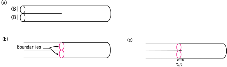
Figure 4: (a) Putting boundary states at two legs of trousers that is associated with three string vertex. (b) Stripping two legs at the origin. (c) Shifting the interaction point as a regularization.

The matrix element $\Phi_{1}\cdot(\Phi_{2}\star\Phi_{3})$ corresponds to putting three local operators $\Phi_{i}$ ($i=1,2,3$) at the ends of three half cylinders.

As we see previously, the boundary states are not described by local operators but should be interpreted as the surface state. To take the product of two boundary states $|B\rangle\star|B\rangle$ is then geometrically represented as the Mandelstam diagram whose two legs are stripped at the interaction time $\tau=0$ (see a Fig. 4-b).

This configuration is, however, singular since two boundaries are attached at one point (interaction point) and we need a regularization to obtain a smooth surface. A natural regularization is to shift the location of the boundary slightly, for example at $\tau=\tau_{1}/2>0$ (Fig. 4-c). As we see later, this is equivalent to a cut-off of the Neumann matrix with finite size $K$ which was used in our previous paper [7]. The correspondence of the regulator turns out to be $K\sim\tau_{1}^{-1}$ . With this regularization, the world-sheet becomes a cylinder with one vertex operator insertion. The limit $\tau_{1}\rightarrow 0$ is equivalent to shrinking a strip of this diagram and reducing it to a disk. We can use the discussion of factorization as,

$$|B\rangle\star_{\tau_{1}}|B\rangle=\sum_{i}q^{\Delta_{i}}A_{i}(\sigma_{1})A_{i}(\sigma_{2})|B\rangle\,,$$ (2.2)

where again $A_{i}(\sigma_{i})$ belongs to a set of orthonormal operators in the open string Hilbert space with both end attached to a brane specified by $|B\rangle$ and $\sigma_{1,2}$ are the coordinates along the boundary.

For the consistency of boundary states of the bosonic string, the lowest dimensional operator in the Hilbert space is always tachyon state which is written as, $|0\rangle^{\mathrm{m}}\otimes c_{1}|0\rangle^{\mathrm{gh}}$ where $|0\rangle^{\mathrm{m,gh}}$ are $SL(2,R)$ invariant vacuum for the matter and ghost. The conformal dimension of this state is $-1$. Other terms depend on the detail of the boundary state but they always give less singular terms as $q\rightarrow 0$. Similarly, if we $\star$-multiply two different boundary states $|B_{1}\rangle\star|B_{2}\rangle$, the open string sector is described by the Hilbert space of the mixed boundary condition and the lowest dimensional operator always has a dimension $\Delta$ greater than $0$. This simple argument then implies,

$$|B_{\alpha}\rangle\star|B_{\beta}\rangle\sim q^{-1}c(\sigma_{1})(c\partial c)(\sigma_{2})\delta_{\alpha\beta}|B_{\beta}\rangle+\ \mbox{less singular terms in $K$}\,.$$ (2.3)

Although the less singular terms do depend on the background and boundary state, the first term is universal. As we see, the precise structure for ghost and singularity is more involved due to the ghost insertions in the three string vertex and the singular behaviour themselves should be modified in order to obtain the precise agreement with the oscillator computation.

2.2 Computation by conformal mappings

In order to see the degeneration in detail, we consider three surfaces which can be related with each other by conformal mappings (Fig. 5-a,b,c).

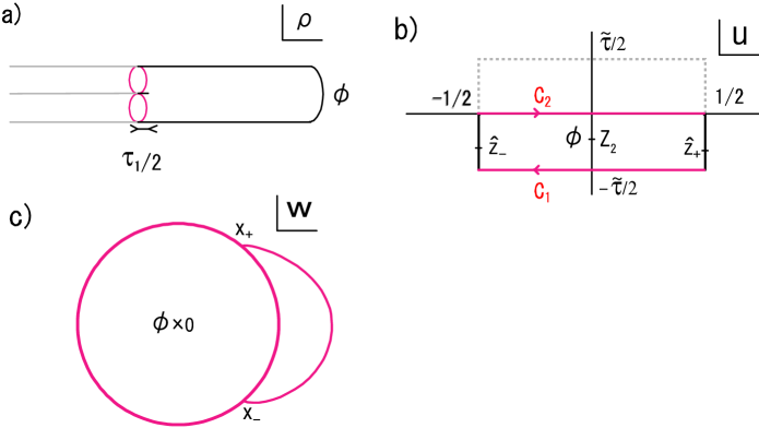
Figure 5: (a) (reguralized) string vertex with two boundary states; (b) a cylinder diagram; (c) a disk diagram with operator insertions.

The first one is the regularized version of the Mandelstam diagram for the star product of two boundary states (Fig. 4-a). A natural coordinate for this diagram is $\rho=\tau+i\sigma$ ($\tau>0$, $-\pi\alpha\leq\sigma\leq\pi\alpha$). The interaction point is $\rho=\tau_{1}/2\pm i\pi\alpha_{1}$, ($0\leq\alpha_{1}\leq\alpha$) and the parameter $\tau_{1}>0$ is introduced for the regularization.

This diagram has two holes together with one vertex operator insertion at infinity. Since it is topologically annulus, it can be mapped to the standard annulus diagram (Fig. 5-b). A complex parameter $u$ ($|\mbox{Re}(u)|\leq 1/2$, $-t/2\leq\mbox{Im}(u)\leq 0$, $\tilde{\tau}:=it$) is a flat complex coordinate and $\tilde{\tau}$ is the moduli parameter. These two diagrams are related with each other by a generalized Mandelstam mapping [21][22],

$$\rho(u)=\alpha\ln\frac{\vartheta_{1}(u-Z_{1}|\tilde{\tau})}{\vartheta_{1}(u-Z_{2}|\tilde{\tau})}-2\pi i\alpha_{1}u\,.$$ (2.4)

We note that it can be extended as a mapping between the doubles of above diagrams, i.e., a torus $-\frac{1}{2}\leq\mbox{Re}(u)\leq\frac{1}{2}$, $-t/2\leq\mbox{Im}(u)\leq t/2$ and corresponding Mandelstam diagram. The parameters $Z_{1,2}:=\mp\beta\tilde{\tau}/2$ are mapped to the infinities $\mbox{Re}(\rho)=\mp\infty$. The interaction point $\tau_{1}/2\mp i\pi\alpha_{1}$ is mapped to $\hat{z}_{\pm}=\pm\frac{1}{2}-\tilde{\tau}y$. There is a set of relations among parameters [22],

$$\beta=-\frac{\alpha_{1}}{\alpha}\,,$$ (2.5)

$$\frac{\tau_{1}}{\alpha}=2\ln\frac{\vartheta_{2}(\tilde{\tau}(-\beta/2+y)|\tilde{\tau})}{\vartheta_{2}(\tilde{\tau}(-\beta/2-y)|\tilde{\tau})}-4\pi i\beta\tilde{\tau}y\,,$$ (2.6)

$$g_{2}(\tilde{\tau}(-\beta/2+y)|\tilde{\tau})+g_{2}(\tilde{\tau}(-\beta/2-y)|\tilde{\tau})=2\pi i\beta\,,$$ (2.7)

where $g_{2}(\nu|\tilde{\tau})=\partial_{\nu}\ln\vartheta_{2}(\nu|\tilde{\tau})$. In the degenerate limit $\tau_{1}\rightarrow 0$, these are reduced to,

$$y\sim\frac{1}{4}\,,\qquad e^{-\frac{i\pi}{\tilde{\tau}}}\equiv q^{1/2}\sim\frac{\tau_{1}}{8\alpha\sin(-\pi\beta)}\,.$$ (2.8)

The third diagram (Fig. 5-c) is disk-like diagram with two short slits. It is parametrized by a complex coordinate $w$ with $|w|\leq 1$. The relation with the Mandelstam diagram is very simple,

$$w=f(\rho)\equiv\exp(-\rho/\alpha)\,.$$ (2.9)

Two slits are located at $x_{\pm}=\exp(\pm\pi i\alpha_{1}/\alpha)=\exp(\mp\pi i\beta)$.

Each diagram has its own role in the computation of $|B\rangle\star|B\rangle$. Firstly, the Mandelstam diagram gives the definition of the star product. The expression,

$$\mathcal{F}\equiv\left(\langle B_{1}|_{\tau_{1}\over 2\alpha_{1}}b^{+}_{0}c_{0}^{-}\star\langle B_{2}|_{\tau_{1}\over 2\alpha_{2}}b^{+}_{0}c_{0}^{-}\right)|\phi\rangle\quad(\langle B|_{T}\equiv\langle B|e^{-T(L_{0}+\bar{L}_{0})})\,,$$ (2.10)

can be evaluated as the one point function of $\phi$ inserted at $\tau=\infty$ in $\rho$-plane with two boundaries defined by $|B_{1,2}\rangle$. $b_{0}^{+}$ insertion is used to cancel $c_{0}^{+}$ factor contained in the boundary state and to set the ghost number to be two. The ket vector $|\phi\rangle=\phi(0)|0\rangle$ has ghost number two as usual. If we map it to the standard annulus diagram (Fig. 5-b), it can be rewritten as,

$$\mathcal{F} = \alpha_{1}\alpha_{2}\langle B_{1}|\tilde{q}^{{1\over 2}(L_{0}+\tilde{L}_{0})}\,b_{\rho}^{+}\,(\rho^{-1}\!\circ\phi)(Z_{2})\,b_{\rho}^{+}|B_{2}\rangle\,,$$ (2.12)

$$\tilde{q}:=e^{2\pi i\tilde{\tau}}\,,~{}~{}~{}~{}b_{\rho}^{+}=\oint\frac{du}{2\pi i}b(u)\left(\frac{d\rho}{du}\right)^{-1}+c.c.\,.$$

We need to evaluate this expression in the limit $\tilde{\tau}\rightarrow 0$ and take the conformal transformation to disk diagram (Fig. 5-c).

As we have argued, taking the limit corresponds to taking the lowest dimensional operator in the open string channel. Therefore, one can rewrite $\mathcal{F}$ in this limit as, (after the conformal map to $w$ plane),

$$\mathcal{F}\sim\delta_{12}\langle B|b_{w}^{1+}b_{w}^{2+}(g\circ c)(x_{+})(g\circ c\partial c)(x_{-})|\phi\rangle\,,$$ (2.13)

where $x_{\pm}=e^{\mp i\pi\beta}$ are the locations of tachyon insertions and $g=f\circ\rho$. $b^{1+}_{w}$ and $b^{2+}_{w}$ are the conformal transformations of $b_{\rho}^{+}$ along two boundaries. The ghost insertions become very complicated but we have already proved in the oscillator formulation [7] that

$$\langle B|b_{w}^{1+}b_{w}^{2+}(g\circ c)(x_{+})(g\circ c\partial c)(x_{-})\sim\langle B|c_{0}^{-}\,.$$ (2.14)

In order to fix the coefficient, we take the simplest example, $|\phi\rangle=c_{1}\tilde{c}_{1}|0\rangle$ and calculate both sides of the equation.

It is convenient to divide the computation into matter and ghost sectors. Let us first consider the matter part. The vertex operator for $|\phi\rangle$ is simply 1. The inner product between two boundary states is

$$\langle B^{\mathrm{m}}_{1}|{\tilde{q}}^{{1\over 2}\left(L_{0}+\tilde{L}_{0}-{c\over 12}\right)}|B^{\mathrm{m}}_{2}\rangle=q^{-{c\over 24}}\,\delta_{12}+\mbox{(higher order in $q$)}\,,$$ (2.15)

where we have supposed that these boundary states $|B_{1}^{\rm m}\rangle,|B_{2}^{\rm m}\rangle$ satisfy Cardy condition and used the leading behavior of the character of identity operator $\chi_{1}(q)\simeq q^{-{c\over 24}}$ ($q\rightarrow 0$). On the other hand, the right hand side becomes,

$$\langle B^{\mathrm{m}}_{2}|0\rangle=T_{B_{2}}\,.$$ (2.16)

Namely the tension for the D-brane [23].

For the ghost part, we compute ${\cal F}$ (2.12) with $\phi=c\tilde{c}$ and take the limit of ${\tilde{\tau}}\rightarrow+i0$ after modular transformation. In order to compute explicitly, we map the $u$-plane to $\tilde{\rho}=2\pi iu$ such that $\tilde{\rho}$-plane becomes closed string strip with period $2\pi$ in the ${\rm Im}\tilde{\rho}$ direction and then we expand the ghosts as

$$b(\tilde{\rho})=\sum_{n=-\infty}^{\infty}b_{n}e^{-n\tilde{\rho}}\,,~{}~{}~{}c(\tilde{\rho})=\sum_{n=-\infty}^{\infty}c_{n}e^{-n\tilde{\rho}}\,,~{}~{}~{}\{b_{n},c_{m}\}=\delta_{n+m,0}\,,~{}~{}~{}~{}~{}~{}$$ (2.17)

and similar ones for $\tilde{b}(\bar{\tilde{\rho}})$ and $\tilde{c}(\bar{\tilde{\rho}})$. Using the property of the boundary states in the ghost sector: $(b_{n}-\tilde{b}_{-n})|B\rangle=0$, we calculate ghost contribution for ${\cal F}$ (2.12) as

$${\cal F}_{c\tilde{c}} = 4\alpha_{1}\alpha_{2}(2\pi)^{2}\int_{C_{1}}{du_{1}\over 2\pi i}{du_{1}\over d\rho}\int_{C_{2}}{du_{2}\over 2\pi i}{du_{2}\over d\rho}\left[\left.{du\over dw_{3}}\right|_{w_{3}=0}\left.{d\bar{u}\over d\bar{w}_{3}}\right|_{\bar{w}_{3}=0}\right]^{-1}$$ (2.18)

$$\times\,\langle B|\tilde{q}^{{1\over 2}\left(L_{0}+\tilde{L}_{0}+{13\over 6}\right)}b(2\pi iu_{1})c(2\pi iZ_{2})\tilde{c}(-2\pi i\bar{Z}_{2})b(2\pi iu_{2})|B\rangle\,.~{}~{}~{}~{}~{}$$

($C_{1}$ and $C_{2}$ are given in Fig. 5-b.) Here the conformal factor $C_{c\tilde{c}}$ for $c\tilde{c}$ (given by $[\cdots]^{-1}$ in the integrand) can be evaluated using the Mandelstam map (2.4) with $\rho(u)=\alpha_{3}\log w_{3}$ ($\alpha_{3}=-\alpha_{1}-\alpha_{2}=-\alpha$) for string $3$ region where $\phi$ is inserted:

$$C_{c\tilde{c}}=\left|{\vartheta_{1}(Z_{2}-Z_{1}|\tilde{\tau})\over\vartheta_{1}^{\prime}(0|\tilde{\tau})}e^{i\pi\tilde{\tau}\beta^{2}}\right|^{-2}\sim\pi^{2}|\tilde{\tau}|^{-2}(\sin\pi\beta)^{-2}\,,~{}~{}~{}(\tilde{\tau}\rightarrow+i0)\,.$$ (2.19)

We have used modular transformation for $\vartheta$-function in order to obtain the last expression. The above inner product $\langle B|\cdots|B\rangle$ is computed straightforwardly:

$$\langle B|\tilde{q}^{{1\over 2}\left(L_{0}+\tilde{L}_{0}+{13\over 6}\right)}b(2\pi iu_{1})c(2\pi iZ_{2})\tilde{c}(-2\pi i\bar{Z}_{2})b(2\pi iu_{2})|B\rangle$$ (2.20)

$$= {-i\over 8\pi}\,e^{i\pi\tilde{\tau}\over 6}\prod_{n=1}^{\infty}(1-e^{2\pi i\tilde{\tau}n})^{2}\,\bigl{[}g_{1}(u_{1}-Z_{1}|\tilde{\tau})-g_{1}(u_{1}-Z_{2}|\tilde{\tau})-g_{1}(u_{2}-Z_{1}|\tilde{\tau})+g_{1}(u_{2}-Z_{2}|\tilde{\tau})\bigr{]}$$

$$= {-i\over 8\pi\alpha}\,\eta(\tilde{\tau})^{2}\left[{d\rho\over du}(u_{1})-{d\rho\over du}(u_{2})\right],$$

where we have used

$$g_{1}(\nu|\tau):={\vartheta_{1}^{\prime}(\nu|\tau)\over\vartheta_{1}(\nu|\tau)}=\pi\cot\pi\nu+4\pi\sum_{n=1}^{\infty}{e^{2\pi in\tau}\over 1-e^{2\pi in\tau}}\sin(2\pi n\nu)\,,$$ (2.21)

$$L_{0}:=\sum_{n=1}^{\infty}n(c_{-n}b_{n}+b_{-n}c_{n})-1\,,~{}~{}\tilde{L}_{0}:=\sum_{n=1}^{\infty}n(\tilde{c}_{-n}\tilde{b}_{n}+\tilde{b}_{-n}\tilde{c}_{n})-1\,,~{}~{}~{}~{}~{}~{}~{}~{}$$ (2.22)

and adopted the normalization as:

$$|B\rangle=e^{\sum_{n=1}^{\infty}(c_{-n}\tilde{b}_{-n}+\tilde{c}_{-n}b_{-n})}c_{0}^{+}c_{1}\tilde{c}_{1}|0\rangle\,,~{}~{}~{}~{}~{}\langle 0|c_{-1}\tilde{c}_{-1}c_{0}\tilde{c}_{0}c_{1}\tilde{c}_{1}|0\rangle=1\,.$$ (2.23)

We note that (2.20) corresponds to (5.16) in [22] which was calculated as the correlation function at the 1-loop of open string, as expected. We perform contour integration for $b$-ghost in (2.18) and reduce it to evaluation of the residue at the interaction point $\hat{z}_{\pm}$ on $u$-plane, where ${d\rho\over du}=0$, by deforming the contour $C_{1}+C_{2}$:

$${\cal F}_{c\tilde{c}} = {2\pi\alpha_{1}\alpha_{2}\over\alpha}\,C_{c\tilde{c}}\,\eta(\tilde{\tau})^{2}\,{\cal R}\,,$$ (2.24)

$${\cal R} = \left(\left.{d^{2}\rho\over du^{2}}\right|_{u=\hat{z}_{\pm}}\right)^{-1}={1\over\alpha}\left(g^{\prime}_{1}(\hat{z}_{\pm}-Z_{1}|\tilde{\tau})-g^{\prime}_{1}(\hat{z}_{\pm}-Z_{2}|\tilde{\tau})\right)^{-1}.~{}~{}~{}~{}$$ (2.25)

In the degenerate limit, using (2.8), the above residue ${\cal R}$ behaves as

$${\cal R} \sim {1\over 4\alpha}\,(\log q)^{-2}\,{q^{-1/2}\over\sin\pi\beta}\,.$$ (2.26)

Then, from $\eta(\tilde{\tau})^{2}=i\tilde{\tau}^{-1}\eta(-1/\tilde{\tau})^{2}\sim|\tilde{\tau}|^{-1}e^{-{\pi\over 6|\tilde{\tau}|}}$ and (2.19), the ghost contribution to ${\cal F}$ with $\phi=c\tilde{c}$ is evaluated as

$${\cal F}_{c\tilde{c}}\sim{-\alpha_{1}\alpha_{2}\over 16\alpha^{2}}\,(\log q)\,q^{13\over 12}\left(q^{-1/2}\over\sin\pi\beta\right)^{3}$$ (2.27)

in the degenerating limit. On the other hand, the inner product of the right hand side of (2.14) and $\phi=c\tilde{c}$ gives

$$\langle B|c_{0}^{-}c_{1}\tilde{c}_{1}|0\rangle=1\,,$$ (2.28)

in the ghost sector.

After combining contributions from the matter and the ghost sector, we note that there is a constraint $\alpha=2p^{+}$ in order to get physical amplitudes [24]. Namely, the string length parameter $\alpha$ should be identified with a light cone momentum $p^{+}$. It gives extra factor $(\log q)^{-1}$ compared to the right hand side in (2.15). (See, (5.41) in [22].) Taking into account of it in open string description, ${\cal F}$ (2.12) is evaluated as

$${\cal F}_{c\tilde{c}} \sim \delta_{12}\,{-\alpha_{1}\alpha_{2}\over 16\alpha^{2}}\,q^{26-c\over 24}\left(q^{-1/2}\over\sin\pi\beta\right)^{3}$$ (2.29)

$$\sim 32\,\delta_{12}\,\alpha_{1}\alpha_{2}(\alpha_{1}+\alpha_{2})\tau_{1}^{-3},$$

where we have substituted $c=26$ as total central charge in the matter sector and used (2.8) in the second line.

After all, using the above results: (2.29),(2.16) and (2.28) for $\phi=c\tilde{c}$, we can evaluate the proportional constant of $B_{1}\star B_{2}\propto\delta_{12}B_{2}$ for Cardy states:

$$\left(\langle B_{1}|_{\tau_{1}\over 2\alpha_{1}}b^{+}_{0}c_{0}^{-}\star\langle B_{2}|_{\tau_{1}\over 2\alpha_{2}}b^{+}_{0}c_{0}^{-}\right)|\phi\rangle/\langle B_{2}|b_{0}^{+}c_{0}^{-}c_{0}^{+}|\phi\rangle \sim 32\,\delta_{12}\,\alpha_{1}\alpha_{2}(\alpha_{1}+\alpha_{2})\tau_{1}^{-3}\,T_{B_{2}}^{-1}\,,$$ (2.30)

with regularization parameter $\tau_{1}$. This implies ${\cal C}\sim 32\,\delta_{12}\,\alpha_{1}\alpha_{2}(\alpha_{1}+\alpha_{2})\tau_{1}^{-3}$ in (1.6) and is consistent with the result in [8] by identifying a regularization parameter $\tau_{1}$ with $K^{-1}$ [8].

2.3 Algebra of Ishibashi states and fusion ring

Before we proceed, we point out that the idempotency relation implies that Ishibashi state satisfies a simple algebra with the $\star$ product. We have discussed such relation in our previous paper [9] by assuming the relation for the generic background. Since it is proved in this paper, it is worth mentioning the result again with a slight generalization.

We focus on the matter part of the idempotency relation (1.6) which may be written as,

$$|a\rangle\star|b\rangle=q^{-{c\over 24}}\,\delta_{ab}\,T_{b}^{-1}|b\rangle\,.$$ (2.31)

Here $q\,(\rightarrow 0)$ is a regularization parameter which was introduced in the previous subsection. The factor $q^{-\frac{c}{24}}$ will contribute, when we combine it with ghost fields with other matter sector, to a universal divergent factor. We will therefore drop it in the following discussion to illuminate the nature of the algebra.

For the rational conformal field theory, the relation between Cardy state with Ishibashi states, (with slight generalization after [25] eq. (2.10)),

$$|a\rangle=\sum_{j}\frac{\psi_{a}^{j}}{\sqrt{S_{j1}}}|j\rangle\!\rangle\,.$$ (2.32)

The coefficient $\psi_{a}^{j}$ should satisfy the orthogonality (eqs. (2.18) (2.19) of [25]),

$$\sum_{a}\psi_{a}^{i}(\psi_{a}^{j})^{*}=\delta_{ij}\,,\quad\sum_{i}\psi_{a}^{i}(\psi_{b}^{i})^{*}=\delta_{ab}\,,\quad$$ (2.33)

and also generalized Verlinde formula (2.16):

$$n_{ia}{}^{b}=\sum_{j}\frac{S_{ij}}{S_{1j}}\psi^{j}_{a}(\psi^{j}_{b})^{*}\,,$$ (2.34)

where $n_{ia}{}^{b}$ are non-negative integers. With this combination, the tension $T_{a}$ can be written as

$$T_{a}=\frac{\psi^{1}_{a}}{\sqrt{S_{11}}}\,.$$ (2.35)

The idempotency relation between Cardy states (in matter sector) can be rewritten as the algebra between the Ishibashi states $|i\rangle\!\rangle$,

$$|i\rangle\!\rangle^{\prime}\star|j\rangle\!\rangle^{\prime}=\sum_{k}\mathcal{N}_{ij}{}^{k}|k\rangle\!\rangle^{\prime}\,,$$ (2.36)

where we changed the normalization of Ishibashi states as,

$$|i\rangle\!\rangle^{\prime}\equiv(S_{i1}S_{11})^{-1/2}|i\rangle\!\rangle\,,$$ (2.37)

and ${\cal N}_{ij}^{~{}~{}k}$ is given by

$$\mathcal{N}_{ij}^{~{}~{}k} = \sum_{a}{(\psi^{i}_{a})^{*}(\psi^{j}_{a})^{*}\psi^{k}_{a}\over\psi^{1}_{a}}\,.$$ (2.38)

Eq. (2.36) is a natural generalization of the fusion ring for the generic BCFT, namely the coefficient $\mathcal{N}_{ij}{}^{k}$ is also known to be non-negative integers [25]. This relation looks natural since (generalized) fusion ring describes the number of channels in OPE of primary fields and Ishibashi states are directly related with the irreducible representation.

One may summarize the observation as, Cardy states are projectors of (generalized) fusion ring. We believe that this nonlinear relation is a natural replacement of Cardy condition in the first quantized language.

As a preparation of the next section, we present an application of this result to the orbifold CFT [9]. We consider an orbifold $\mathbf{R}^{d}/\Gamma$ where $\Gamma$ is a finite group which may be nonabelian in general. At the orbifold singularity, there exist fractional D-branes which are given as combinations of various twisted sector. We apply the above idea to these fractional D-branes.

In this setup, there is a boundary state which belongs to the twisted sector specified by $h\in\Gamma$,

$$(X(\sigma+2\pi)-h\cdot X(\sigma))|h\rangle\!\rangle=0\,.$$ (2.39)

When $\Gamma$ is nonabelian, however, such a state is not invariant under conjugation. Ishibashi state is, therefore, given as a linear combination of such boundary state which belongs to a conjugacy class $C_{j}$ of $\Gamma$:

$$|j\rangle\!\rangle:={1\over\sqrt{r_{j}}}\sum_{h_{j}\in C_{j}}|h_{j}\rangle\!\rangle,$$ (2.40)

where $r_{j}$ is the number of elements in $C_{j}$.

In this case, Cardy state $|a\rangle$ is given by eq. (2.32) where the coefficients $\psi^{j}_{a}$, $S_{j1}$ are [26]

$$\psi_{a}^{j}=\sqrt{r_{j}\over|\Gamma|}\,\zeta^{(a)}_{j},~{}~{}~{}~{}~{}S_{j1}={1\over\sigma(e,h_{j})},~{}~{}(h_{j}\in C_{j})\,,$$ (2.41)

$\zeta^{(a)}_{j}$ is the character of an irreducible representation $a$ for $g\in C_{j}$, $e$ is the identity element of $\Gamma$ and $\sigma(e,h)$ is determined by the modular transformation of the character $\chi_{g}^{h}(q)\equiv{\rm Tr}_{{\cal H}_{g}}(h\,q^{L_{0}-{c\over 24}})$:

$$\chi_{e}^{h}(q)=\sigma(e,h)\chi_{h}^{e}(\tilde{q})\,,~{}~{}~{}~{}(q=e^{2\pi i\tau},~{}\tilde{q}=e^{-{2\pi i\over\tau}})\,.$$ (2.42)

The normalization of Ishibashi state $|h\rangle\!\rangle$ is specified as $\langle\!\langle h|\tilde{q}^{{1\over 2}\left(L_{0}+\tilde{L}_{0}-{c\over 12}\right)}|h\rangle\!\rangle=\chi_{h}^{e}(\tilde{q})\,.$ In this case, eq. (2.36) is equivalent to

$$e_{i}\star e_{j}=\sum_{k}{\cal N}_{ij}^{~{}~{}k}\,e_{k}\,,~{}~{}~{}~{}{\cal N}_{ij}^{~{}~{}k}=\sum_{a}{r_{i}r_{j}\zeta_{i}^{(a)}\zeta_{j}^{(a)}\zeta_{k}^{(a)*}\over\zeta_{1}^{(a)}}\,,$$ (2.43)

$$e_{i}:=|\Gamma|\sqrt{r_{i}\,\sigma(e,h_{i})}\,|i\rangle\!\rangle\,.$$ (2.44)

Namely the (generalized) fusion ring is equivalent to the group ring ${\bf C}^{[\Gamma]}$ [27].

The example in the next section is a simple example of this general algebra. The orbifold group $\Gamma$ is ${\bf Z}_{2}$ and we have only two Ishibashi states in untwisted and twisted sector. We write them as $|+\rangle\!\rangle$ and $|-\rangle\!\rangle$. The above algebra (2.43) is simply,

$$e_{\pm}\star e_{\pm}=e_{+}\,,\quad e_{\pm}\star e_{\mp}=e_{-}\,,$$ (2.45)

$$e_{+}:=2|+\rangle\!\rangle\,,\quad e_{-}:=2\sqrt{\sigma(e,g)}\,|-\rangle\!\rangle\,,~{}~{}{\bf Z}_{2}=\{e,g\}\,,$$ (2.46)

(using $\sigma(e,e)=1$) and its idempotents $P_{\pm}$ are easily obtained:

$$P_{\pm}={1\over 2}(e_{+}\pm e_{-})=|+\rangle\!\rangle\pm\sqrt{\sigma(e,g)}\,|-\rangle\!\rangle\,,$$ (2.47)

which is the same as the Cardy states (2.32) up to overall factor.

3 Explicit computation: toroidal and $Z_{2}$ orbifold compactifications

As nontrivial examples of general arguments in the previous section, we calculate the $\star$ product between Ishibashi states on torus and $Z_{2}$ orbifold. We use explicit oscillator representations of three string vertices which were formulated in [17] and [18], respectively. These simple examples contain nontrivial ingredients such as winding modes, twisted sector, cocycle factor, etc. which make the explicit computation more interesting compared to ${\bf R}^{d}$ case in [7].

We use ${\bf R}^{d}\times T^{D}$ and ${\bf R}^{d}\times T^{D}/{\bf Z}_{2}$ as a background spacetime and consider the HIKKO $\star$ product on them. For the torus $T^{D}$, we identify its coordinates as $X^{i}\sim X^{i}+2\pi\sqrt{\alpha^{\prime}}~{}(i=1,\cdots,D)$ and introduce constant background metric $G_{ij}$ and antisymmetric tensor $B_{ij}$. In the case of $Z_{2}$ orbifold $T^{D}/{\bf Z}_{2}$, the action of ${\bf Z}_{2}$ is defined by $X^{i}\rightarrow-X^{i}~{}(i=1,\cdots,D)$. The ghost sector and ${\bf R}^{d}$ sector of the star product are the same as the original HIKKO’s construction [6]. We will compute the star product of string fields of the form $|\Phi(\alpha)\rangle=|B_{D}\rangle\otimes|\Phi_{B}(x^{\perp},\alpha)\rangle$, where $|B_{D}\rangle$ is boundary states in $D$-dimensional sector: $T^{D}$ or $T^{D}/{\bf Z}_{2}$ and $|\Phi_{B}(x^{\perp},\alpha)\rangle=c_{0}^{-}b_{0}^{+}\,|B\rangle_{\rm matter}\otimes|B\rangle_{\rm ghost}\otimes|\alpha\rangle$ represents a boundary state for D-brane at $x^{\perp}(\in{\bf R}^{d-p-1})$ including ghost and $\alpha$-sector. For the ${\bf R}^{d}$ sector, conventional boundary states for D$p$-brane were proved to be idempotent in [7, 8]:

$$|\Phi_{B}(x^{\perp},\alpha_{1})\rangle\star|\Phi_{B}(y^{\perp},\alpha_{2})\rangle$$

$$~{}=~{}\delta^{d-p-1}(x^{\perp}-y^{\perp})\,\mu^{2}\,{\det}^{-{d-2\over 2}}(1-(\tilde{N}^{33})^{2})\,c_{0}^{+}|\Phi_{B}(x^{\perp},\alpha_{1}+\alpha_{2})\rangle,~{}~{}~{}~{}$$ (3.1)

$$\mu=e^{-\tau_{0}\sum_{r=1}^{3}\alpha_{r}^{-1}},~{}~{}~{}\tau_{0}=\sum_{r=1}^{3}\alpha_{r}\log|\alpha_{r}|,~{}~{}~{}(\alpha_{3}\equiv-\alpha_{2}-\alpha_{1})\,.$$ (3.2)

In this section, we will focus on the matter $T^{D}$ or $T^{D}/{\bf Z}_{2}$ sector and prove a similar relation for Cardy states on those backgrounds.

By toroidal compactification, winding mode is introduced in addition to momentum; the zero mode sector $|p\rangle$ changes to $|p,w\rangle$ with $p_{i},w^{i}\in{\bf Z}$. Due to this mode, the boundary states and the 3-string vertex should be modified. The definition of the boundary state will be given in (3.5). The 3-string vertex should be modified to include “cocycle factor” such as $e^{-i\pi(p_{3}w_{2}-p_{1}w_{1})}$. (See, Appendix A for detail.) It is necessary to guarantee “Jacobi identity” with respect to closed string fields :

$$(\Phi_{1}\star\Phi_{2})\star\Phi_{3}+(-1)^{|\Phi_{1}|(|\Phi_{2}|+|\Phi_{3}|)}(\Phi_{2}\star\Phi_{3})\star\Phi_{1}+(-1)^{|\Phi_{3}|(\Phi_{1}|+|\phi_{2}|)}(\Phi_{3}\star\Phi_{1})\star\Phi_{2} = 0\,,~{}~{}$$ (3.3)

which plays an important role to prove gauge invariance of the action of closed string field theory [17]. It can be also derived by careful treatment of the connection condition of light-cone type in [28]. When the boundary state has non-vanishing winding number, this cocycle factor becomes relevant.

$T^{D}/{\bf Z}_{2}$ is one of the simplest examples of orbifold background on which we gave a general argument in [9] and previous subsection (§2.3). Cardy state $|a_{\pm}\rangle$ (2.32, 2.47), which represents fractional D-brane, is given by:

$$|a_{\pm}\rangle={1\over\sqrt{2}}\left(|\iota\rangle\!\rangle_{u}\pm 2^{D\over 4}|\iota\rangle\!\rangle_{t}\right),$$ (3.4)

where $|\iota\rangle\!\rangle_{u}$ or $|\iota\rangle\!\rangle_{t}$ is a linear combination of Ishibashi states in the untwisted or twisted sector, respectively. The ratio of coefficients $2^{D\over 4}$ comes from the factor $\sqrt{\sigma(e,g)}$ for $T^{D}/{\bf Z}_{2}$. We will demonstrate that string fields given in (3.32) which are of the above form satisfy idempotency relations (3.28, 3.29). It provides a consistency check for the previous general arguments. The oscillator computation, however, has a limitation in determining coefficients of Ishibashi state. They are given by determinants of infinite rank Neumann matrices and are divergent in general. As a regularization, we slightly shift the interaction time which is specified by overlapping of three strings as we discussed in §2.2. We reduce the ratio of determinants to the degenerating limit of the ratio of 1-loop amplitudes in the sense of (D.5).

We will also comment on compatibility of idempotency relations on $T^{D}$ and $T^{D}/{\bf Z}_{2}$ with T-duality transformation in string field theory which was investigated in [24] for $T^{D}$.

3.1 Star product between Ishibashi states

In this subsection, we first introduce Ishibashi states $|\iota\rangle\!\rangle$ for the backgrounds $T^{D}$ and $T^{D}/{\bf Z}_{2}$ and then compute the star product between them. In Appendix A, we give some definitions and our convention of free oscillators.

Ishibashi states

The Ishibashi states $|\iota\rangle\!\rangle$ for the torus $T^{D}$ are obtained by solving $(\alpha^{i}_{n}+{\cal O}^{i}_{~{}j}\tilde{\alpha}_{-n}^{j})|\iota\rangle\!\rangle=0$. ${\cal O}^{i}_{~{}j}$ is an orthogonal matrix in the sense ${\cal O}^{T}G{\cal O}=G$. Explicitly it is written as

$$|\iota({\cal O},p,w)\rangle\!\rangle=e^{-\sum_{n=1}^{\infty}{1\over n}\alpha_{-n}^{i}G_{ij}{\cal O}^{j}_{~{}k}\tilde{\alpha}^{k}_{-n}}|p,w\rangle\,,~{}~{}p_{i}=-2\pi\alpha^{\prime}F_{ij}w^{j}\,,$$ (3.5)

with labels of momentum $p_{i}$ and winding number $w^{j}$ . The antisymmetric matrix $F_{ij}$ is given by ${\cal O}=(E^{T}-2\pi\alpha^{\prime}F)^{-1}(E+2\pi\alpha^{\prime}F)$ (where $E_{ij}:=G_{ij}+2\pi\alpha^{\prime}B_{ij}$). It must be quantized in order to keep $p_{i}$ and $w^{j}$: integers with a relation $(1+{\cal O}^{T-1})p-(E-{\cal O}^{T-1}E^{T})w=0$, which corresponds to $(\alpha_{0}^{i}+{\cal O}^{i}_{~{}j}\tilde{\alpha}_{0}^{j})|\iota\rangle\!\rangle=0$. In particular, for Dirichlet type boundary condition, we should set $w^{i}=0$ since ${\cal O}=-1$.

For $T^{D}/{\bf Z}_{2}$, there are Ishibashi states in untwisted and twisted sectors. For the untwisted sector, they can be obtained by multiplying ${\bf Z}_{2}$-projection to the ones for the torus:

$${\cal P}_{u}^{Z_{2}}|\iota({\cal O},p,w)\rangle\!\rangle_{u}={1\over 2}(|\iota({\cal O},p,w)\rangle\!\rangle_{u}+|\iota({\cal O},-p,-w)\rangle\!\rangle_{u})\,,$$ (3.6)

where we add a subscript $u$ to make a distinction from the Ishibashi states for the torus. For the twisted sector, we have Ishibashi states of the form:

$$|\iota({\cal O},n^{f})\rangle\!\rangle_{t} = e^{-\sum_{r=1/2}^{\infty}{1\over r}\alpha_{-r}^{i}G_{ij}{\cal O}^{j}_{~{}k}\tilde{\alpha}^{k}_{-r}}|n^{f}\rangle\,.$$ (3.7)

The label $(n^{f})^{i}$ takes value $0$ or $1$ and specifies a fixed point. This state has ${\bf Z}_{2}$ invariance: ${\cal P}^{Z_{2}}_{t}|\iota({\cal O},n^{f})\rangle\!\rangle_{t}=|\iota({\cal O},n^{f})\rangle\!\rangle_{t}$.

$\star$ product

For $T^{D}$ case, the $\star$ product of the states (3.5) becomes:

$$|\iota({\cal O},p_{1},w_{1})\rangle\!\rangle_{\alpha_{1}}\star|\iota({\cal O},p_{2},w_{2})\rangle\!\rangle_{\alpha_{2}}$$

$$=~{}{\det}^{-{D\over 2}}(1-(\tilde{N}^{33})^{2})\,(-1)^{p_{1}w_{2}}|\iota({\cal O},p_{1}+p_{2},w_{1}+w_{2})\rangle\!\rangle_{\alpha_{1}+\alpha_{2}}\,,$$ (3.8)

where we have assigned $\alpha_{r}$ for each string (we consider the case of $\alpha_{1}\alpha_{2}>0$ here and following) and omitted the ghost and the matter ${\bf R}^{d}$ sector. Differences from ${\bf R}^{d}$ case [7] are limited to the existence of winding mode and the cocycle factor and the proof is similar; we use eqs. (A.7) and (A.10) without ${\cal P}^{Z_{2}}_{u1}{\cal P}^{Z_{2}}_{u2}{\cal P}^{Z_{2}}_{u3}$. The cocycle factor appeared as an extra sign factor $(-1)^{p_{1}w_{2}}=(-1)^{w_{1}(2\pi\alpha^{\prime}F)w_{2}}$. We note that this factor is irrelevant for the Dirichlet type boundary state since we need to set $w=0$.

For $T^{D}/{\bf Z}_{2}$, we have to compute three combinations of Ishibashi states: $({\rm untwisted})\star({\rm untwisted})$, $({\rm twisted})\star({\rm twisted})$ and $({\rm untwisted})\star({\rm twisted})$. The first one can be obtained by ${\bf Z}_{2}$-projection of the torus case (3.1):

$${\cal P}^{Z_{2}}_{u}|\iota({\cal O},p_{1},w_{1})\rangle\!\rangle_{u,\alpha_{1}}\star{\cal P}^{Z_{2}}_{u}|\iota({\cal O},p_{2},w_{2})\rangle\!\rangle_{u,\alpha_{2}}$$

$$={\det}^{-{D\over 2}}(1-(\tilde{N}^{33})^{2})\,{(-1)^{p_{1}w_{2}}\over 2}\,{\cal P}^{Z_{2}}_{u}$$ (3.9)

$$~{}~{}~{}\times\left[|\iota({\cal O},p_{1}+p_{2},w_{1}+w_{2})\rangle\!\rangle_{u,\alpha_{1}+\alpha_{2}}+|\iota({\cal O},p_{1}-p_{2},w_{1}-w_{2})\rangle\!\rangle_{u,\alpha_{1}+\alpha_{2}}\right].$$

The star product for two Ishibashi states (3.7) in the twisted sector can be computed by the vertex operators (A.9, A) (with appropriate permutation such that string $3$ is in the untwisted sector). Using the identities among Neumann coefficients given in (B.5), a direct computation which is similar to that in [7] yields

$$|\iota({\cal O},n_{1}^{f})\rangle\!\rangle_{t,\alpha_{1}}\star|\iota({\cal O},n_{2}^{f})\rangle\!\rangle_{t,\alpha_{2}}$$ (3.10)

$$=~{}e^{{D\over 8}\tau_{0}(\alpha_{1}^{-1}+\alpha_{2}^{-1})}{\det}^{-{D\over 2}}(1-(\tilde{T}^{3_{u}3_{u}})^{2})\wp{\cal P}^{Z_{2}}_{u}\sum_{p,w}\gamma({\bf p};n_{1}^{f},n_{2}^{f})\,e^{\Delta E}\,e^{-\sum_{n>0}{1\over n}\alpha_{-n}{\cal O}\tilde{\alpha}_{-n}}|p,w\rangle_{\alpha_{1}+\alpha_{2}}\,,$$

where

$$\Delta E = -\sum_{n>0}n^{-{1\over 2}}(\alpha_{-n}+\tilde{\alpha}_{-n}{\cal O}^{T})\sum_{r,s=1,2}\,\sum_{m_{r},l_{s}>0}\tilde{T}^{3_{u}r}_{nm_{r}}[(\tilde{T}^{\,\cdot\,3_{u}}\tilde{T}^{3_{u}\cdot})^{-1}]^{rs}_{m_{r}l_{s}}\tilde{T}^{s3_{u}}_{l_{s}0}{\bf p}_{+}$$ (3.11)

$$+{1\over 4}\left(T^{3_{u}3_{u}}_{00}-\sum_{r,s=1,2}\,\sum_{n_{r},m_{s}>0}\tilde{T}^{3_{u}r}_{0n_{r}}[(1+\tilde{T})^{-1}]^{rs}_{n_{r}m_{s}}\tilde{T}^{s3_{u}}_{m_{s}0}\right){\bf p}_{+}G^{-1}{\bf p}_{+}\,,$$

$$({\bf p}_{+})_{i} = {1\over\sqrt{2}}[(1+{\cal O}^{T-1})p-(E-{\cal O}^{T-1}E^{T})w]_{i}\,.$$ (3.12)

The above peculiar exponent $\Delta E$ can be ignored because the coefficient of positive definite factor ${\bf p}_{+}G^{-1}{\bf p}_{+}$ can be evaluated by using various formulae in Appendix B as

$$T^{3_{u}3_{u}}_{00}-\sum_{r,s=1,2}\,\sum_{n_{r},m_{s}>0}\tilde{T}^{3_{u}r}_{0n_{r}}[(1+\tilde{T})^{-1}]^{rs}_{n_{r}m_{s}}\tilde{T}^{s3_{u}}_{m_{s}0} = -\sum_{n=1}^{\infty}{2\cos^{2}\left({\alpha_{1}\over\alpha_{3}}n\pi\right)\over n}\,.~{}~{}~{}~{}~{}~{}~{}~{}$$ (3.13)

Since it gives $-\infty$, the ${\bf p}_{+}\neq 0$ terms in the summation in (3.10) is suppressed. The constraint ${\bf p}_{+}=0$ implies $p_{i}=-2\pi\alpha^{\prime}F_{ij}w^{j}$ in (3.5), which is consistent with $(L_{n}-\tilde{L}_{-n})\left(|\iota({\cal O},n_{1}^{f})\rangle\!\rangle_{t,\alpha_{1}}\star|\iota({\cal O},n_{2}^{f})\rangle\!\rangle_{t,\alpha_{2}}\right)=0$. This is an example of our general claim in Ref. [8] that the star product between the conformal invariant states is again conformal invariant; $(L_{n}-\tilde{L}_{-n})|B_{i}\rangle=0,i=1,2,\forall n\in{\bf Z}$  $\rightarrow$  $(L_{n}-\tilde{L}_{-n})(|B_{1}\rangle\star|B_{2}\rangle)=0$. The final form of the $\star$ product becomes,

$$|\iota({\cal O},n_{1}^{f})\rangle\!\rangle_{t,\alpha_{1}}\star|\iota({\cal O},n_{2}^{f})\rangle\!\rangle_{t,\alpha_{2}}$$ (3.14)

$$=~{}e^{{D\over 8}\tau_{0}(\alpha_{1}^{-1}+\alpha_{2}^{-1})}{\det}^{-{D\over 2}}(1-(\tilde{T}^{3_{u}3_{u}})^{2})\sum_{p,w,{\bf p}_{+}=0}(-1)^{p\,n_{2}^{f}}\sum_{m}\delta^{D}_{n_{2}^{f}-n_{1}^{f}+w+2m,0}|\iota({\cal O},p,w)\rangle\!\rangle_{u,\alpha_{1}+\alpha_{2}}\,.$$

Finally the $\star$ product between the Ishibashi states in untwisted and twisted sectors can be computed similarly by using the formulae in (B.5):

$${\cal P}_{u}^{Z_{2}}|\iota({\cal O},p_{1},w_{1})\rangle\!\rangle_{u,\alpha_{1}}\star|\iota({\cal O},n_{2}^{f})\rangle\!\rangle_{t,\alpha_{2}}$$

$$=~{}e^{{D\over 8}\tau_{0}(\alpha_{2}^{-1}-(\alpha_{1}+\alpha_{2})^{-1})}\,{\det}^{-{D\over 2}}(1-(\tilde{T}^{3_{t}3_{t}})^{2})\,(-1)^{p_{1}n_{2}^{f}}|\iota({\cal O},[n_{2}^{f}-w_{1}]_{{\rm mod}\,2})\rangle\!\rangle_{t,\alpha_{1}+\alpha_{2}}\,.$$ (3.15)

We have similar formula for [twisted(3.7)] $\star$ [untwisted(3.6)] by appropriate replacement in the above.

We have confirmed that Ishibashi states on ${\bf Z}_{2}$ orbifold (3.6) and (3.7) (resp., on torus (3.5)) form a closed algebra with respect to the $\star$ product as eqs. (3.1),(3.14) and (3.15) (resp., eq. (3.1)).

3.2 Cardy states as idempotents

We proceed to compare the Cardy state and idempotent of $\star$ product algebra (fusion ring) for Ishibashi state that we have just computed. We note that the algebra for the Dirichlet type boundary states are simpler since there is no winding number and consequently the cocycle factor in the vertex operator vanishes. Because of this simplicity we divide our discussion into Dirichlet and Neumann type boundary states.

Dirichlet type

We start our consideration from Dirichlet type states, namely ${\cal O}^{i}_{~{}j}=-\delta^{i}_{j}$ for the torus. The Cardy state which describes the Dirichlet boundary condition is given by a Fourier transformation of Ishibashi states (3.5) with respect to momentum $p_{i}$:

$$|B(x)\rangle = \left(\det(2G_{ij})\right)^{-{1\over 4}}\sum_{p\in{\bf Z}^{D}}e^{-ix^{i}p_{i}}|\iota(-1,p,0)\rangle\!\rangle\,.$$ (3.16)

One can check that it satisfies $[\alpha^{\prime-{1\over 2}}X^{i}(\sigma)-x^{i}]_{\rm mod\,2\pi}|B(x)\rangle=0$. We have chosen its normalization by

$$\langle B(x)|q^{{1\over 2}(L_{0}+\tilde{L}_{0}-{D\over 12})}|B(x^{\prime})\rangle = \eta(\tau)^{-D}\left[{\det}^{-{1\over 2}}(2G_{ij})\sum_{p\in{\bf Z}^{D}}e^{-i(x-x^{\prime})p}q^{{1\over 4}pG^{-1}p}\right]$$ (3.17)

$$= \eta(-1/\tau)^{-D}\sum_{m\in{\bf Z}^{D}}e^{-{i\over 2\pi\tau}(x-x^{\prime}+2\pi m)G(x-x^{\prime}+2\pi m)}\,,$$

where $q=e^{2\pi i\tau}$ and $\eta(\tau)=q^{1\over 24}\prod_{n=1}^{\infty}(1-q^{n})$. The last representation implies that it gives 1-loop amplitude of open string whose boundaries are on D-branes at $x$ and $x^{\prime}$ on the torus $T^{D}$.

On the other hand, from (3.1), the star product between them becomes

$$|B(x)\rangle_{\alpha_{1}}\star|B(x^{\prime})\rangle_{\alpha_{2}}$$ (3.18)

$$=~{}\delta^{D}([x-x^{\prime}])(2\pi)^{D}\left(\det(2G_{ij})\right)^{-{1\over 4}}{\det}^{-{D\over 2}}(1-(\tilde{N}^{33})^{2})\,|B(x)\rangle_{\alpha_{1}+\alpha_{2}}\,,$$

where $\delta^{D}([x-x^{\prime}]):=\sum_{m\in{\bf Z}^{D}}\delta^{D}(x-x^{\prime}+2\pi m)=(2\pi)^{-D}\sum_{p\in{\bf Z}^{D}}e^{-i(x-x^{\prime})p}$. This is the idempotency relation in [7] for the toroidal compactification.

For $T^{D}/{\bf Z}_{2}$, the boundary state with ${\bf Z}_{2}$ projection, ${{\cal P}^{Z_{2}}_{u}}|B(x)\rangle_{u}={1\over 2}(|B(x)\rangle_{u}+|B(-x)\rangle_{u})$ gives idempotents in the sense:

$${{\cal P}^{Z_{2}}_{u}}|B(x)\rangle_{u,\alpha_{1}}\star{{\cal P}^{Z_{2}}_{u}}|B(x^{\prime})\rangle_{u,\alpha_{2}}$$ (3.19)

$$=\,{1\over 2}\,(\delta^{D}([x-x^{\prime}])+\delta^{D}([x+x^{\prime}]))(2\pi)^{D}\left(\det(2G_{ij})\right)^{-{1\over 4}}{\det}^{-{D\over 2}}(1-(\tilde{N}^{33})^{2})\,{{\cal P}^{Z_{2}}_{u}}|B(x)\rangle_{u,\alpha_{1}+\alpha_{2}}\,.$$

It is clear that the combination of delta functions is well-defined on $T^{D}/{\bf Z}_{2}$.

At the fixed point, there are fractional D-branes. To see them, we consider a restriction of $x$ to a fixed point $\pi n^{f}$,

$$|B_{n^{f}}\rangle_{u} = \left(\det(2G_{ij})\right)^{-{1\over 4}}\sum_{p\in{\bf Z}^{D}}(-1)^{p\,n^{f}}|\iota(-1,p,0)\rangle\!\rangle_{u},$$ (3.20)

it is ${\bf Z}_{2}$ invariant by itself ${\cal P}^{Z_{2}}_{u}|B_{n^{f}}\rangle_{u}=|B_{n^{f}}\rangle_{u}$ and is idempotent:

$$|B_{n^{f}_{1}}\rangle_{u,\alpha_{1}}\star|B_{n^{f}_{2}}\rangle_{u,\alpha_{2}}$$

$$~{}=(2\pi\delta(0))^{D}\delta^{D}_{n_{1}^{f},n_{2}^{f}}\left(\det(2G_{ij})\right)^{-{1\over 4}}\,{\det}^{-{D\over 2}}(1-(\tilde{N}^{33})^{2})\,|B_{n^{f}_{1}}\rangle_{u,\alpha_{1}+\alpha_{2}}.~{}~{}~{}~{}~{}~{}~{}$$ (3.21)

For the twisted sector, we can derive from eqs. (3.14), (3.15) and (3.20),

$$|B_{n_{1}^{f}}\rangle_{t,\alpha_{1}}\star|B_{n_{2}^{f}}\rangle_{t,\alpha_{2}}$$

$$=\delta^{D}_{n_{1}^{f},n_{2}^{f}}\left(\det(2G_{ij})\right)^{1\over 4}e^{{D\over 8}\tau_{0}(\alpha_{1}^{-1}+\alpha_{2}^{-1})}{\det}^{-{D\over 2}}(1-(\tilde{T}^{3_{u}3_{u}})^{2})\,|B_{n^{f}_{1}}\rangle_{u,\alpha_{1}+\alpha_{2}}\,,$$ (3.22)

$$|B_{n_{1}^{f}}\rangle_{u,\alpha_{1}}\star|B_{n_{2}^{f}}\rangle_{t,\alpha_{2}}$$

$$=\delta^{D}_{n_{1}^{f},n_{2}^{f}}\left(\det(2G_{ij})\right)^{-{1\over 4}}(2\pi\delta(0))^{D}\,e^{{D\over 8}\tau_{0}(\alpha_{2}^{-1}-(\alpha_{1}+\alpha_{2})^{-1})}{\det}^{-{D\over 2}}(1-(\tilde{T}^{3_{t}3_{t}})^{2})\,|B_{n^{f}_{1}}\rangle_{t,\alpha_{1}+\alpha_{2}}\,,~{}~{}~{}~{}~{}~{}~{}$$ (3.23)

where $|B_{n^{f}}\rangle_{t}:=|\iota(-1,n^{f})\rangle\!\rangle_{t}$. These eqs. (3.21),(3.22) and (3.23) show that the Dirichlet boundary states at fixed points, $|B_{n^{f}}\rangle_{u}$ and $|B_{n^{f}}\rangle_{t}$, form a closed algebra with respect to the $\star$ product. It can be diagonalized by taking a linear combination of the untwisted and twisted sectors:

$$|\Phi_{B}(n^{f},x^{\perp},\alpha)\rangle_{\pm}$$ (3.24)

$$={1\over 2}(2\pi\delta(0))^{-D}\left({\det}^{1\over 4}(2G_{ij})|B_{n^{f}}\rangle_{u}\pm c_{t}(2\pi\delta(0))^{D\over 2}|B_{n^{f}}\rangle_{t}\right)\otimes|\Phi_{B}(x^{\perp},\alpha)\rangle,$$

where we have included a string field $|\Phi_{B}(x^{\perp},\alpha)\rangle$, which is a contribution from the other part of matter sector ${\bf R}^{d}$ and ghost sector. It is essentially a boundary state for D$p$-brane. The coefficient of the boundary states in the twisted sector is given by a ratio of the determinants of Neumann matrices:

$$c_{t} := \sqrt{{\cal C}\over{\cal C}^{\prime}}=\left(e^{-{\tau_{0}\over 4}(\alpha_{1}^{-1}+\alpha_{2}^{-1})}\,{\det(1-(\tilde{T}^{3_{u}3_{u}})^{2})\over\det(1-(\tilde{N}^{33})^{2})}\right)^{D\over 4},$$ (3.25)

$${\cal C} = \mu^{2}\,{\det}^{-{d+D-2\over 2}}(1-(\tilde{N}^{33})^{2})\,,~{}~{}~{}~{}\mu=e^{-\tau_{0}(\alpha_{1}^{-1}+\alpha_{2}^{-1}-(\alpha_{1}+\alpha_{2})^{-1})},~{}~{}~{}$$ (3.26)

$${\cal C}^{\prime} = \mu^{2}\,e^{{D\over 8}\tau_{0}(\alpha_{1}^{-1}+\alpha_{2}^{-1})}{\det}^{-{D\over 2}}(1-(\tilde{T}^{3_{u}3_{u}})^{2})\,{\det}^{-{d-2\over 2}}(1-(\tilde{N}^{33})^{2})\,.$$ (3.27)

They satisfy idempotency relations of the following form:

$$|\Phi_{B}(n_{1}^{f},x^{\perp},\alpha_{1})\rangle_{\pm}\star|\Phi_{B}(n_{2}^{f},y^{\perp},\alpha_{2})\rangle_{\pm}$$

$$~{}~{}~{}=~{}\delta^{D}_{n_{1}^{f},\,n_{2}^{f}}\,\delta^{d-p-1}(x^{\perp}-y^{\perp})\,{\cal C}\,c_{0}^{+}|\Phi_{B}(n_{1}^{f},x^{\perp},\alpha_{1}+\alpha_{2})\rangle_{\pm}\,,$$ (3.28)

$$|\Phi_{B}(n_{1}^{f},x^{\perp},\alpha_{1})\rangle_{\pm}\star|\Phi_{B}(n_{2}^{f},y^{\perp},\alpha_{2})\rangle_{\mp}=0\,,$$ (3.29)

where ${\cal C}$ was computed in [8] and is proportional to $K^{3}\alpha_{1}\alpha_{2}(\alpha_{1}+\alpha_{2})$ for $d+D=26$ with cutoff parameter $K$. In the above computation, we have used the relation of determinants of Neumann matrices:

$${\det}^{-{1\over 2}}(1-(\tilde{N}^{33})^{2})=e^{{1\over 8}\tau_{0}(\alpha_{2}^{-1}-(\alpha_{1}+\alpha_{2})^{-1})}{\det}^{-{1\over 2}}(1-(\tilde{T}^{3_{t}3_{t}})^{2})\,,$$ (3.30)

which can be proved analytically by using Cremmer-Gervais identity as in Ref. [8]. Outline of the proof is given in Appendix C. It can be also checked numerically by truncating the size of Neumann matrices to $L\times L$. ($L\sim K$)

As for the coefficient $c_{t}$ (3.25) in front of the twisted sector, it can be evaluated by another regularization as §2.2 (See, Appendix D for detail.) The result is given in (D.5):

$$c_{t}(2\pi\delta(0))^{D\over 2}=2^{D\over 4}\left(\det(2G)\right)^{1\over 4}=\sqrt{\sigma(e,g)}\left(\det(2G)\right)^{1\over 4}\,,$$ (3.31)

where $\sigma(e,g)=2^{D\over 2}$ is the Modular transformation matrix defined in (2.42) and is given in [26]. This implies that the idempotents (3.24) is proportional to the Cardy state for the fractional D-branes,

$$|\Phi_{B}(n^{f},x^{\perp},\alpha)\rangle_{\pm}={1\over 2}\,{{\det}^{1\over 4}(2G)\over(2\pi\delta(0))^{D}}\left(|B_{n^{f}}\rangle_{u}\pm 2^{D\over 4}|B_{n^{f}}\rangle_{t}\right)\otimes|\Phi_{B}(x^{\perp},\alpha)\rangle,~{}~{}~{}~{}~{}~{}$$ (3.32)

after a proper regularization.

Neumann type

We call the boundary states with ${\cal O}^{i}_{~{}j}\neq-\delta^{i}_{j}$ as Neumann type while they may have mixed boundary condition in general. As we wrote, the derivation of idempotent for such states is slightly more nontrivial because of the cocycle factor in the vertex.

We start again from the toroidal compactification and consider a particular linear combination of Ishibashi states (3.5) of the form:

$$|B(q),F\rangle:={\det}^{-{1\over 4}}(2G_{O}^{-1})\sum_{w}e^{-iqw+i\pi wF_{u}w}|\iota({\cal O},-2\pi\alpha^{\prime}Fw,w)\rangle\!\rangle\,,$$ (3.33)

where we denote $(F_{u})_{ij}=2\pi\alpha^{\prime}F_{ij}$ for $i<j$ and $(F_{u})_{ij}=0$ for $i\geq j$. As we explained, $2\pi\alpha^{\prime}F_{ij}$ should be quantized for the consistency with the momentum quantization. We have chosen the normalization factor ${\det}^{-{1\over 4}}(2G_{O}^{-1})$ by

$$\langle B(q^{\prime}),F|\,e^{\pi i\tau\left(L_{0}+\tilde{L}_{0}-{D\over 12}\right)}|B(q),F\rangle = {\det}^{-{1\over 2}}(2G_{O}^{-1})\,\eta(\tau)^{-D}\sum_{w^{i}}e^{-i(q-q^{\prime})_{i}w^{i}}e^{{\pi i\tau\over 2}w^{i}G_{Oij}w^{j}}$$ (3.34)

$$= \eta(-1/\tau)^{-D}\sum_{m}e^{-{i\over 2\pi\tau}(q-q^{\prime}+2\pi m)_{i}G_{O}^{ij}(q-q^{\prime}+2\pi m)_{j}}\,,$$

as (3.17). Here $q_{i}\equiv q_{i}+2\pi$ corresponds to Wilson line on the D-brane and ${G_{O}}_{ij}:=G_{ij}-(E+2\pi\alpha^{\prime}F)_{ik}G^{kl}(E^{T}-2\pi\alpha^{\prime}F)_{lj}$ is the open string metric.

We compute the $\star$ product of (3.33) using (3.1):

$$|B(q_{1}),F\rangle_{\alpha_{1}}\star|B(q_{2}),F\rangle_{\alpha_{2}}$$ (3.35)

$$~{}=\delta^{D}([q_{1}-q_{2}])\,(2\pi)^{D}{\det}^{-{1\over 4}}(2G_{O}^{-1})\,{\det}^{-{D\over 2}}(1-(\tilde{N}^{33})^{2})\,|B(q_{1}),F\rangle_{\alpha_{1}+\alpha_{2}},$$

which is the idempotency relation for $T^{D}$. We note that due the phase factor $e^{i\pi wF_{u}w}$ in (3.33), Cardy state is not the Fourier transform of the Ishibashi state. It is necessary to cancel the cocycle factor in the 3-string vertex (A.10). It is also necessary to keep T-duality symmetry in closed string field theory on the torus $T^{D}$, (see, eq. (3.55) in particular).

For the orbifold, we can check that ${\cal P}^{Z_{2}}_{u}|B(q),F\rangle_{u}={1\over 2}(|B(q),F\rangle_{u}+|B(-q),F\rangle_{u})$ is idempotent in the untwisted sector on $T^{D}/{\bf Z}_{2}$:

$${{\cal P}^{Z_{2}}_{u}}|B(q),F\rangle_{u,\alpha_{1}}\star{{\cal P}^{Z_{2}}_{u}}|B(q^{\prime}),F\rangle_{u,\alpha_{2}}$$ (3.36)

$$~{}~{}=~{}{1\over 2}(\delta^{D}([q-q^{\prime}])+\delta^{D}([q+q^{\prime}]))(2\pi)^{D}{\det}^{-{1\over 4}}(2G_{O}^{-1}){\det}^{-{D\over 2}}(1-(\tilde{N}^{33})^{2})\,{{\cal P}^{Z_{2}}_{u}}|B(q),F\rangle_{u,\alpha_{1}+\alpha_{2}}\,.$$

Mixing with the twisted sector occurs when the Wilson line takes special values, $q_{i}=\pi m^{f}_{i}$ ($m_{i}^{f}=0,1$) for the untwisted sector:

$$|B_{m^{f}},F\rangle_{u}={\det}^{-{1\over 4}}(2G_{O}^{-1})\sum_{w}(-1)^{m^{f}w+wF_{u}w}|\iota({\cal O},-2\pi\alpha^{\prime}Fw,w)\rangle\!\rangle_{u}\,.~{}~{}~{}~{}~{}~{}~{}~{}$$ (3.37)

These states are by themselves ${\bf Z}_{2}$ invariant: ${\cal P}^{Z_{2}}_{u}|B_{m^{f}},F\rangle_{u}=|B_{m^{f}},F\rangle_{u}$. The star product between them is,

$$|B_{m^{f}_{1}},F\rangle_{u,\alpha_{1}}\star|B_{m^{f}_{2}},F\rangle_{u,\alpha_{2}}$$ (3.38)

$$~{}=\delta^{D}_{m^{f}_{1},m^{f}_{2}}{\det}^{-{1\over 4}}(2G_{O}^{-1})(2\pi\delta(0))^{D}{\det}^{-{D\over 2}}(1-(\tilde{N}^{33})^{2})\,|B_{m^{f}_{1}},F\rangle_{u,\alpha_{1}+\alpha_{2}}\,.$$

In the twisted sector, we consider a particular linear combination of Ishibashi states (3.7) such as

$$|B_{m^{f}},F\rangle_{t}:=2^{-{D\over 2}}\sum_{n^{f}_{i}=0,1}(-1)^{m^{f}n^{f}+n^{f}F_{u}n^{f}}|\iota({\cal O},n^{f})\rangle\!\rangle_{t}\,,$$ (3.39)

which is a generalization of the twisted Neumann boundary state in [29]. Here, we have also multiplied the phase factor $(-1)^{n^{f}F_{u}n^{f}}$ as in the untwisted sector (3.37) for the idempotency. We can derive the $\star$ product formulae

$$|B_{m_{1}^{f}},F\rangle_{t,\alpha_{1}}\star|B_{m^{f}_{2}},F\rangle_{t,\alpha_{2}}$$ (3.40)

$$=\delta^{D}_{m^{f}_{1},\,m^{f}_{2}}{\det}^{1\over 4}(2G_{O}^{-1})\,e^{{D\over 8}\tau_{0}(\alpha_{1}^{-1}+\alpha_{2}^{-1})}{\det}^{-{D\over 2}}(1-(\tilde{T}^{3_{u}3_{u}})^{2})|B_{m^{f}_{1}},F\rangle_{u,\alpha_{1}+\alpha_{2}},$$

$$|B_{m_{1}^{f}},F\rangle_{u,\alpha_{1}}\star|B_{m_{2}^{f}},F\rangle_{t,\alpha_{2}}$$ (3.41)

$$=\delta_{m_{1}^{f},\,m_{2}^{f}}{\det}^{-{1\over 4}}(2G_{O}^{-1})(2\pi\delta(0))^{D}e^{{D\over 8}\tau_{0}(\alpha_{2}^{-1}-(\alpha_{1}+\alpha_{2})^{-1})}{\det}^{-{D\over 2}}(1-(\tilde{T}^{3_{t}3_{t}})^{2})\,|B_{m_{1}^{f}},F\rangle_{t,\alpha_{1}+\alpha_{2}},$$

from eqs. (3.14),(3.15),(3.37) and (3.39). Using the above formulae, noting eq. (3.30), we obtain idempotents which include the twisted sector:

$$|\Phi_{B}(m^{f},F,x^{\perp},\alpha)\rangle_{\pm}={1\over 2}\,{{\det}^{1\over 4}(2G_{O}^{-1})\over(2\pi\delta(0))^{D}}\left(|B_{m^{f}},F\rangle_{u}\pm 2^{D\over 4}\,|B_{m^{f}},F\rangle_{t}\right)\otimes|\Phi_{B}(x^{\perp},\alpha)\rangle\,.~{}~{}~{}$$ (3.42)

Here we again include the extra matter fields on ${\bf R}^{d}$ and ghost sector: $|\Phi_{B}(x^{\perp},\alpha)\rangle$. We evaluate the ratio of determinants $c_{t}$ (3.25) using the regularization given by (D) instead of (D) because we are treating Neumann type boundary states. Their star product becomes idempotent as expected,

$$|\Phi_{B}(m_{1}^{f},F,x^{\perp},\alpha_{1})\rangle_{\pm}\star|\Phi_{B}(m_{2}^{f},F,y^{\perp},\alpha_{2})\rangle_{\pm}$$

$$~{}~{}~{}=~{}\delta^{D}_{m_{1}^{f},\,m_{2}^{f}}\,\delta^{d-p-1}(x^{\perp}-y^{\perp})\,{\cal C}\,c_{0}^{+}|\Phi_{B}(m_{1}^{f},x^{\perp},\alpha_{1}+\alpha_{2})\rangle_{\pm}\,,$$ (3.43)

$$|\Phi_{B}(m_{1}^{f},x^{\perp},\alpha_{1})\rangle_{\pm}\star|\Phi_{B}(m_{2}^{f},y^{\perp},\alpha_{2})\rangle_{\mp}=0\,.$$ (3.44)

3.3 Comments on T-duality

We have seen that the Dirichlet type idempotent and the Neumann type one are constructed in slightly different manner due to the cocycle factor. They are related, however, by T-duality transformation and we would like to see explicitly how the difference can be absorbed. In this subsection we follow the argument of [24].

A key ingredient is the existence of the following operator $\mathcal{U}_{g}^{\dagger}$,

$${\cal U}_{g}^{\dagger}|A\star B\rangle_{E} = |({\cal U}_{g}^{\dagger}A)\star({\cal U}_{g}^{\dagger}B)\rangle_{g(E)}\,.$$ (3.45)

Here the subscripts of the ket: $E$ and $g(E)$ specify the constant background $E=G+2\pi\alpha^{\prime}B$ and its T-duality transformation specified by $g\in O(D,D;{\bf Z})$:

$$g(E):=(aE+b)(cE+d)^{-1},$$ (3.46)

$$g=\left(\begin{array}[tb]{cc}a&b\\ c&d\end{array}\right),~{}~{}~{}~{}g^{T}Jg=g\,,~{}J:=\left(\begin{array}[tb]{cc}0&1_{D}\\ 1_{D}&0\end{array}\right).$$ (3.51)

The operator ${\cal U}_{g}$ is defined by [24]:

$${\cal U}_{g}=U_{g}\,\Upsilon(g,\hat{p},\hat{w})\,,~{}~{}U_{g}^{\dagger}|p,w\rangle_{E}=|ap+bw,cp+dw\rangle_{g(E)},$$ (3.52)

$$U_{g}^{\dagger}\alpha_{n}(E)U_{g}=(d-cE^{T})^{-1}\alpha_{n}(g(E))\,,$$ (3.53)

$$U_{g}^{\dagger}\tilde{\alpha}_{n}(E)U_{g}=(d+cE)^{-1}\tilde{\alpha}_{n}(g(E))\,,~{}~{}~{}~{}~{}$$ (3.54)

$$\Upsilon(g,\hat{p},\hat{w})=\exp(i\pi(\hat{p}(dc^{T})_{u}\hat{p}+\hat{w}(ba^{T})_{u}\hat{w}+\hat{w}bc^{T}\hat{p}))\,,$$ (3.55)

where matrices in the exponent of $\Upsilon$ with subscript $u$ are defined by $(A_{u})_{ij}=A_{ij}\,(i<j)$ and $(A_{u})_{ij}=0\,(i\geq j)$. In particular, we consider a class of $O(D,D;{\bf Z})$-transformation of the form:

$$g_{\rm DN} = \left(\begin{array}[tb]{cc}-2\pi\alpha^{\prime}F&1\\ 1&0\end{array}\right)\,,~{}~{}~{}~{}~{}~{}(2\pi\alpha^{\prime}F_{ij}=-2\pi\alpha^{\prime}F_{ji}\in\mathbf{Z}).$$ (3.58)

They give T-duality transformations between the idempotents

$${\cal U}_{g_{\rm DN}}^{\dagger}|B(x^{i})\rangle_{E}=|B(q_{i}=x^{i}),F\rangle_{g_{\rm DN}(E)}\,,$$ (3.59)

on the torus. Note that the original metric $G$ is mapped to the inverse open string metric $G^{-1}_{O}$ by the transformation $g_{\rm DN}$:

$$G=(E^{\prime T}-2\pi\alpha^{\prime}F)^{-1}G^{\prime}(E^{\prime}+2\pi\alpha^{\prime}F)^{-1}=G^{\prime-1}_{O}\,,~{}~{}~{}~{}~{}E^{\prime}=g_{\rm DN}(E)\,.$$ (3.60)

Indeed, this is consistent with general property of the $\star$ product (3.45).

We can extend such an analysis to $T^{D}/{\bf Z}_{2}$ case. We define a unitary operator ${\cal U}_{g_{\rm DN}}$ which represent the action of $g_{\rm DN}$ (3.58) to the twisted sector:

$${\cal U}_{g_{\rm DN}}^{\dagger}\alpha_{r}(E){\cal U}_{g_{\rm DN}} = -E^{T-1}\alpha_{r}(g_{\rm DN}(E)),$$ (3.61)

$${\cal U}_{g_{\rm DN}}^{\dagger}\tilde{\alpha}_{r}(E){\cal U}_{g_{\rm DN}} = E^{-1}\tilde{\alpha}_{r}(g_{\rm DN}(E)),$$ (3.62)

where $\alpha_{r}(E),~{}(r\in{\bf Z}+{1/2})$ is the oscillator on the background $E$. For the oscillator vacuum $|n^{f}\rangle_{E}$, we define

$${\cal U}^{\dagger}_{g_{\rm DN}}|n^{f}\rangle_{E} = 2^{-{D\over 2}}\sum_{m^{f}_{i}=0,1}(-1)^{n^{f}_{i}m^{f}_{i}+m^{f}_{i}(F_{u})_{ij}m^{f}_{j}}|n^{f}\rangle_{g_{\rm DN}(E)}\,.$$ (3.63)

Then, with ${\bf Z}_{2}$ projection, we can prove

$${\cal U}^{\dagger}_{g_{\rm DN}}|A\star B\rangle_{E}=|({\cal U}^{\dagger}_{g_{\rm DN}}A)\star({\cal U}^{\dagger}_{g_{\rm DN}}B)\rangle_{g_{\rm DN}(E)},$$ (3.64)

not only in the untwisted sector but also in the twisted sector by investigating reflectors (A.7),(A.9) and 3-string vertices (A.10),(A). This implies that we obtain Neumann type idempotents (3.42) from Dirichlet type (3.24) by ${\cal U}^{\dagger}_{g_{\rm DN}}$:

$${\cal U}^{\dagger}_{g_{\rm DN}}|\Phi_{B}(n^{f}_{i},x^{\perp},\alpha)\rangle_{\pm,E}=|\Phi_{B}(m^{f}_{i}=n^{f}_{i},F,x^{\perp},\alpha)\rangle_{\pm,\,g_{\rm DN}(E)}\,.$$ (3.65)

4 Deformation of the algebra by $B$ field

In this section, we consider a deformation along the transverse directions by the introduction of $B$ field. In Seiberg-Witten limit, it induces noncommutativity to the ring of functions on these directions. Since our equation, $\Phi\star\Phi=\Phi$ formally resembles GMS soliton equation, it is curious how our star product is modified in such limit.

In particular, the algebra of Ishibashi state in transverse dimension was,

$$|p\rangle\!\rangle\star|q\rangle\!\rangle=a(p,q)|{p+q}\rangle\!\rangle\,,\quad(a(p,q)=1)$$ (4.1)

when there is no $B$ field. In order to obtain a projector for this algebra, we perform a Fourier transformation $|x^{\perp}\rangle=\int dk\,e^{ikx^{\perp}}|k\rangle\!\rangle$, which combines Ishibashi states to Cardy state, and this is identical to the the boundary state for the transverse direction.

A naive guess is that the product becomes Moyal product, namely $a(p,q)$ becomes $\exp\left(-\frac{i}{2}p_{i}\theta^{ij}q_{j}\right)$. This can not, however, be the case since the closed string star product is commutative. We will see that in a specific setup which we are going to consider, the factor becomes

$$a(p,q)=\frac{\sin(-\beta\lambda)}{-\beta\lambda}\frac{\sin((1+\beta)\lambda)}{(1+\beta)\lambda}\,,\quad\lambda=-{1\over 2}\,p_{i}\theta^{ij}q_{j}\,,$$ (4.2)

for HIKKO type star product in the Seiberg-Witten limit. If we expand in terms of $\lambda$, it is easy to see that this expression reduces to $1$ when $\theta\rightarrow 0$. It is commutative and non-associative which are the basic properties of closed string star product.

If we know the boundary state in the presence of $B$ field in the transverse dimensions, our computation would be straightforward since the definition of the star product itself remains the same. Actually, however, the boundary state which corresponds to GMS soliton is not known. Namely, the treatment of the massive particles is difficult. Such modes can be decoupled from zero-mode only when Seiberg-Witten limit is taken.

Therefore, we are going to take the following path to obtain the deformation of the algebra,

1. define an operator $V_{\theta}$ (4.3) which describes the deformation by $B$ field and apply that operator to Ishibashi states, $|p\rangle\!\rangle^{\prime}=V_{\theta}|p\rangle\!\rangle$,

2. calculate $\star$ product between these states $|p\rangle\!\rangle^{\prime}\star|q\rangle\!\rangle^{\prime}$,

3. and take Seiberg-Witten limit.

Actually the state obtained in the step 1 does not satisfy the conformal invariance $(L_{n}-\tilde{L}_{-n})|B\rangle=0$. It means that they are not, precisely speaking, the boundary states. Instead, we will see that the deformed Ishibashi state is equivalent to Neumann type boundary state with tachyon vertex insertion (4.21). It may imply that our computation in the following should be related to the loop correction factor in noncommutative Yang-Mills theory.

4.1 A deformation of boundary state in the presence of $B$ field

Let us first introduce “KT-operator” $V_{\theta}=e^{M}$ [30, 31], which defines the deformation associated with the noncommutativity for the constant $B$-field background in Witten’s open string field theory and HIKKO open-closed string field theory. In that context, it was demonstrated that this operator $V_{\theta}$ transforms open string fields on $B=0$ background to that on $B\neq 0$. The KT operator $V_{\theta}$ on a constant metric $g_{ij}$ background is given by

$$V_{\theta} = \exp\left(-{i\over 4}\oint d\sigma\oint d\sigma^{\prime}P_{i}(\sigma)\theta^{ij}\epsilon(\sigma-\sigma^{\prime})P_{j}(\sigma^{\prime})\right)$$ (4.3)

where $P_{i}(\sigma)={1\over 2\pi}\left[\hat{p}_{i}+{1\over\sqrt{2\alpha^{\prime}}}\sum_{n\neq 0,\,n\in{\bf Z}}g_{ij}\left(\alpha_{n}^{j}e^{in\sigma}+\tilde{\alpha}_{n}^{j}e^{-in\sigma}\right)\right]$, and $\epsilon(x)$ is the sign function. Formally, we get

$$V_{\theta}\partial_{\sigma}X^{i}(\sigma)V^{-1}_{\theta}=\partial_{\sigma}X^{i}(\sigma)-\theta^{ij}P_{j}(\sigma)$$ (4.4)

by canonical commutation relation, and therefore, we can expect that the operator $V_{\theta}$ induces a map from Dirichlet boundary state to Neumann one with constant flux.

A subtlety in (4.3) is how to define $\epsilon(\sigma-\sigma^{\prime})$ or $\oint d\sigma\oint d\sigma^{\prime}$ since we need to impose the periodicity of closed strings $P_{i}(\sigma+2\pi)=P_{i}(\sigma)$. Here, we introduce a cut $\sigma_{c}$ and set the integration region to $\sigma\in[\sigma_{c},2\pi+\sigma_{c}]$. Then, by taking normal ordering using a formula given in (E), an explicit oscillator representation of KT operator $V_{\theta}$ (4.3) becomes,

$$V_{\theta,\sigma_{c}} := \exp\left(-{i\over 4}\int_{\sigma_{c}}^{2\pi+\sigma_{c}}d\sigma\int_{\sigma_{c}}^{2\pi+\sigma_{c}}d\sigma^{\prime}P_{i}(\sigma)\theta^{ij}\epsilon(\sigma-\sigma^{\prime})P_{j}(\sigma^{\prime})\right)$$ (4.5)

$$= \left(\det\left(1-C\right)\right)^{-{1\over 2}}e^{{1\over 2}DN(1-C)^{-1}D^{T}}e^{-{1\over 2}a^{\dagger}NC(1+C)^{-1}a^{\dagger}+D(1+C)^{-1}a^{\dagger}}$$

$$\times\,e^{-a^{\dagger}\log(1-C)a}e^{{1\over 2}aNC(1-C)^{-1}a+DN(1-C)^{-1}a},$$

where

$$a=\left(\begin{array}[tb]{c}{(e\alpha_{n})^{a}\over\sqrt{n}}\\ {(e\tilde{\alpha}_{n})^{a}\over\sqrt{n}}\end{array}\right),~{}a^{\dagger}=\left(\begin{array}[tb]{c}{(e\alpha_{-n})^{a}\over\sqrt{n}}\\ {(e\tilde{\alpha}_{-n})^{a}\over\sqrt{n}}\end{array}\right),~{}(n\geq 1);~{}~{}g_{ij}=e_{i}^{a}\eta_{ab}e_{j}^{b}\,,~{}g^{ij}=\tilde{e}^{i}_{a}\eta^{ab}\tilde{e}^{j}_{b}\,,~{}e_{i}^{a}\tilde{e}_{a}^{j}=\delta_{i}^{j},~{}~{}~{}~{}~{}$$ (4.10)

$$C=-C^{T}=-{1\over 4\pi\alpha^{\prime}}\left(\begin{array}[tb]{cc}(e\theta e)^{ab}\delta_{n,m}&0\\ 0&-(e\theta e)^{ab}\delta_{n,m}\end{array}\right),$$ (4.13)

$$N=N^{T}=\left(\begin{array}[tb]{cc}0&\eta_{ab}\delta_{n,m}\\ \eta_{ab}\delta_{n,m}&0\end{array}\right),~{}~{}~{}~{}D=-{1\over 2\pi\sqrt{2\alpha^{\prime}}}\,\hat{p}_{i}\,\theta^{ij}\left(e_{j}^{a}\,{e^{-im\sigma_{c}}\over\sqrt{m}},-e_{j}^{a}\,{e^{im\sigma_{c}}\over\sqrt{m}}\right).$$ (4.16)

By multiplying $V_{\theta,\sigma_{c}}$ (4.5) to the Dirichlet type Ishibashi state with momentum $p$: $|p\rangle\!\rangle_{D}:=e^{\sum_{n\geq 1}{1\over n}\alpha^{i}_{-n}g_{ij}\tilde{\alpha}^{j}_{-n}}|p\rangle$, we obtain

$$V_{\theta,\sigma_{c}}|p\rangle\!\rangle_{D}=\left[\det\left(1-(2\pi\alpha^{\prime})^{-1}g\theta\right)\right]^{-\sum_{n\geq 1}1}\,e^{-\alpha^{\prime}pG^{-1}_{\theta}p\,\sum_{n\geq 1}{1\over n}}$$ (4.17)

$$~{}~{}~{}~{}~{}~{}~{}~{}~{}~{}~{}~{}~{}~{}~{}~{}\times\exp\left(-\sum_{n=1}^{\infty}{1\over n}\alpha_{-n}g{\cal O}_{\theta}\tilde{\alpha}_{-n}+\sum_{n=1}^{\infty}(\lambda_{n}\alpha_{-n}+\tilde{\lambda}_{n}\tilde{\alpha}_{-n})\right)|p\rangle,$$

$${\cal O}_{\theta}=(g+2\pi\alpha^{\prime}\theta^{-1})^{-1}(g-2\pi\alpha^{\prime}\theta^{-1})\,,~{}~{}~{}G^{-1}_{\theta}=(g-2\pi\alpha^{\prime}\theta^{-1})^{-1}g(g+2\pi\alpha^{\prime}\theta^{-1})^{-1},$$ (4.18)

$$(\lambda_{m},\tilde{\lambda}_{m})=\sqrt{2\alpha^{\prime}}\,p\left((g-2\pi\alpha^{\prime}\theta^{-1})^{-1}g\,{e^{-im\sigma_{c}}\over m},(g+2\pi\alpha^{\prime}\theta^{-1})^{-1}g\,{e^{im\sigma_{c}}\over m}\right).$$ (4.19)

We redefine the normalization of this state as

$$\hat{V}_{\theta,\sigma_{c}}|p\rangle\!\rangle_{D}:=\left[\det\left(1-(2\pi\alpha^{\prime})^{-1}g\theta\right)\right]^{\sum_{n\geq 1}1}e^{\alpha^{\prime}pG^{-1}_{\theta}p\,\sum_{n\geq 1}{1\over n}}\,V_{\theta,\sigma_{c}}|p\rangle\!\rangle_{D},$$ (4.20)

so that $\langle p^{\prime}|\hat{V}_{\theta,\sigma_{c}}|p\rangle\!\rangle_{D}=(2\pi)^{d}\delta^{d}(p^{\prime}-p)$. Then, we find an identity

$$\hat{V}_{\theta,\sigma_{c}}|p\rangle\!\rangle_{D} = V_{p}(\sigma_{c})|B(F_{ij}=-(\theta^{-1})_{ij})\rangle\,,$$ (4.21)

where

$$|B(F)\rangle=e^{-\sum_{n=1}^{\infty}{1\over n}\alpha_{-n}g{\cal O}\tilde{\alpha}_{-n}}|p=0\rangle$$ (4.22)

with ${\cal O}=(g-2\pi\alpha^{\prime}F)^{-1}(g+2\pi\alpha^{\prime}F)$, is the Neumann boundary state with constant flux $F$ and

$$V_{k}(\sigma)={\cal N}_{k}:e^{ikX(\sigma)}:$$

$$=e^{{1\over 2}\alpha^{\prime}kG^{-1}_{O}k\sum_{n\geq 1}{1\over n}}\,e^{k\sum_{n=1}^{\infty}\left(\alpha^{\prime}\over 2\right)^{1/2}{1\over n}\left(\alpha_{-n}e^{-in\sigma}+\tilde{\alpha}_{-n}e^{in\sigma}\right)}e^{ik\hat{x}}\,e^{-k\sum_{n=1}^{\infty}\left(\alpha^{\prime}\over 2\right)^{1/2}{1\over n}\left(\alpha_{n}e^{in\sigma}+\tilde{\alpha}_{n}e^{-in\sigma}\right)},~{}~{}~{}~{}~{}~{}~{}$$ (4.23)

where $G_{O}^{-1}=(g+2\pi\alpha^{\prime}F)^{-1}g(g-2\pi\alpha^{\prime}F)^{-1}$ is the open string metric, represents the tachyon vertex operator at $\sigma$ with momentum $k_{i}$.

The above identity (4.21) implies that the KT operator (4.5) maps the Dirichlet type Ishibashi state of momentum $p$ to Neumann boundary states with tachyon vertex with momentum $p$, where the position of the tachyon insertion $\sigma_{c}$ corresponds to the cut in the definition of the exponent of (4.5). This combination was investigated as a fluctuation around boundary states in [7, 8] and can be used to calculate their star product in the following.

4.2 $\star$ product of deformed Ishibashi state

Let us proceed to the step 2, namely the computation of the $\star$ product of $\hat{V}_{\theta,\sigma_{c}}|p\rangle\!\rangle_{D}$ (4.20). We use eqs. (4.6) and (4.7) in [7] to give

$$\hat{V}_{\theta,\sigma_{c}}|p_{1}\rangle\!\rangle_{D,\alpha_{1}}\star\hat{V}_{\theta,\sigma_{c}}|p_{2}\rangle\!\rangle_{D,\alpha_{2}}$$

$$={\cal N}_{12}\,{\det}^{-{d\over 2}}(1-(\tilde{N}^{33})^{2})\oint{d\sigma_{1}\over 2\pi}\oint{d\sigma_{2}\over 2\pi}|e^{i\sigma^{(1)}(\sigma_{1})}-e^{i\sigma^{(2)}(\sigma_{2})}|^{2\alpha^{\prime}p_{1}G^{-1}_{O}p_{2}}\,e^{i\Theta_{12}}$$

$$~{}~{}~{}~{}\times\,\wp\,e^{\sum_{n\geq 1}(\lambda_{n}^{(12)}\alpha_{-n}+\tilde{\lambda}_{n}^{(12)}\tilde{\alpha}_{-n})-{\sum_{n\geq 1}{1\over n}\alpha_{-n}G{\cal O}\tilde{\alpha}_{-n}}}|p_{1}+p_{2}\rangle_{\alpha_{1}+\alpha_{2}}\,,$$ (4.24)

where we have assigned $\alpha_{1},\alpha_{2}$ ($\alpha_{1}\alpha_{2}>0$) and omitted ghost sector. Here, the coordinates $\sigma^{(1)}(\sigma_{1})$ and $\sigma^{(2)}(\sigma_{2})$ are given by

$$\sigma^{(1)}(\sigma_{1}) = {\alpha_{1}\over\alpha_{1}+\alpha_{2}}(\sigma_{c}+\sigma_{1})-\pi\,{\rm sgn}(\sigma_{c}+\sigma_{1})\,,$$ (4.25)

$$\sigma^{(2)}(\sigma_{2}) = {\alpha_{2}\over\alpha_{1}+\alpha_{2}}\left(\sigma_{c}+\sigma_{2}-\pi\,{\rm sgn}(\sigma_{c}+\sigma_{2})\right),$$ (4.26)

for $|\sigma_{c}+\sigma_{r}|<\pi,~{}r=1,2$, which represent the positions of tachyon vertices on the boundary of the joined string $3$ specified by the overlapping condition for the 3-string vertex. Note that the phase factor $e^{i\Theta_{12}}$ appears as a result of the $\star$ product of closed string field theory which is computed from the last term in eq. (4.7) in [7] using (E.3) as

$$\Theta_{12} = -{1\over 2\pi}\,p_{1i}\vartheta^{ij}p_{2j}(\sigma^{(1)}(\sigma_{1})-\sigma^{(2)}(\sigma_{2}))+{1\over 2}p_{1i}\vartheta^{ij}p_{2j}\,\epsilon(\sigma^{(1)}(\sigma_{1})-\sigma^{(2)}(\sigma_{2}))\,,$$ (4.27)

where

$${\vartheta}^{ij}=(2\pi\alpha^{\prime})^{2}\left[(g-2\pi\alpha^{\prime}\theta^{-1})^{-1}{\theta}^{-1}(g+2\pi\alpha^{\prime}\theta^{-1})^{-1}\right]^{ij}$$ (4.28)

corresponds to the noncommutativity parameter. In the exponent, linear terms with respect to oscillators are given by

$$\lambda_{n}^{(12)} = {\sqrt{2\alpha^{\prime}}\over n}\left(p_{1}\,e^{-in\sigma^{(1)}(\sigma_{1})}+p_{2}\,e^{-in\sigma^{(2)}(\sigma_{2})}\right)(g-2\pi\alpha^{\prime}\theta^{-1})^{-1}g\,,~{}~{}$$ (4.29)

$$\tilde{\lambda}_{n}^{(12)} = {\sqrt{2\alpha^{\prime}}\over n}\left(p_{1}\,e^{in\sigma^{(1)}(\sigma_{1})}+p_{2}\,e^{in\sigma^{(2)}(\sigma_{2})}\right)(g+2\pi\alpha^{\prime}\theta^{-1})^{-1}g\,.$$ (4.30)

The factor ${\cal N}_{12}$ is evaluated as

$${\cal N}_{12} = \lim_{L\rightarrow\infty}\left[e^{\alpha^{\prime}p_{1}G^{-1}_{O}p_{1}\left(\sum_{n=1}^{|\alpha_{1}|L}{1\over n}-\sum_{p=1}^{|\alpha_{3}|L}{1\over p}\right)}e^{\alpha^{\prime}p_{2}G^{-1}_{O}p_{2}\left(\sum_{n=1}^{|\alpha_{2}|L}{1\over n}-\sum_{p=1}^{|\alpha_{3}|L}{1\over p}\right)}\right]$$ (4.31)

$$= (-\beta)^{\alpha^{\prime}p_{1}G^{-1}_{O}p_{1}}(1+\beta)^{\alpha^{\prime}p_{2}G^{-1}_{O}p_{2}},~{}~{}~{}(\beta={\alpha_{1}/\alpha_{3}},~{}\alpha_{3}=-\alpha_{1}-\alpha_{2}),$$

where we take cutoffs for the mode number of strings such that they are proportional to each string length parameter $|\alpha_{r}|$. This prescription was used in [7]v4 in order to investigate the on-shell condition from idempotency and is consistent with conformal factor of the open string tachyon vertex [8]. We can also rewrite (4.24) as

$$\hat{V}_{\theta,\sigma_{c}}|p_{1}\rangle\!\rangle_{D,\alpha_{1}}\star\hat{V}_{\theta,\sigma_{c}}|p_{2}\rangle\!\rangle_{D,\alpha_{2}}$$

$$=~{}(-\beta)^{\alpha^{\prime}p_{1}G^{-1}_{O}p_{1}}(1+\beta)^{\alpha^{\prime}p_{2}G^{-1}_{O}p_{2}}\,{\det}^{-{d\over 2}}(1-(\tilde{N}^{33})^{2})$$ (4.32)

$$~{}~{}~{}~{}\times\oint{d\sigma_{1}\over 2\pi}\oint{d\sigma_{2}\over 2\pi}\wp\,V_{p_{1}}(\sigma^{(1)}(\sigma_{1}))V_{p_{1}}(\sigma^{(2)}(\sigma_{2}))|B(F=-\theta^{-1})\rangle_{\alpha_{1}+\alpha_{2}}\,,$$

using tachyon vertex given in (4.23). This implies that the $\star$ product of $\hat{V}_{\theta,\sigma_{c}}|p\rangle\!\rangle_{D}$ induces conventional operator product of tachyon vertices on the Neumann boundary state.

4.3 Seiberg-Witten limit

Next, we proceed the third step to take Seiberg-Witten limit [33] of (4.24) in order to obtain the deformed algebra. In the limit $\alpha^{\prime}\sim\varepsilon^{1\over 2}\rightarrow 0\,,~{}g_{ij}\sim\varepsilon\rightarrow 0$, the $\star$ product formula (4.24) is simplified as

$$\hat{V}_{\theta,\sigma_{c}}|p_{1}\rangle\!\rangle_{D,\alpha_{1}}\star\hat{V}_{\theta,\sigma_{c}}|p_{2}\rangle\!\rangle_{D,\alpha_{2}}\sim a(p_{1},p_{2})\hat{V}_{\theta,\sigma_{c}}|p_{1}+p_{2}\rangle\!\rangle_{D,\alpha_{1}+\alpha_{2}}\,,$$ (4.34)

$$a(p_{1},p_{2})\equiv{\det}^{-{d\over 2}}(1-(\tilde{N}^{33})^{2})\oint{d\sigma_{1}\over 2\pi}\oint{d\sigma_{2}\over 2\pi}\,e^{i\Theta_{12}}\,,$$

where we have estimated using $\alpha^{i}_{-n}=\sqrt{n}\,\tilde{e}^{i}_{a}a^{\dagger a}_{n}\sim\varepsilon^{-{1\over 2}}$ and ignored linear terms in the exponent. We can interprete that, in this limit, the deformed Ishibashi states: $\hat{V}_{\theta,\sigma_{c}}|p\rangle\!\rangle_{D}$ form a closed algebra with respect to the $\star$ product of closed string field theory. After we drop the determinant factor, the coefficient $a(p_{1},p_{2})$ can be evaluated as

$$a(p_{1},p_{2})={\sin(-\beta p_{1i}\theta^{ij}p_{2j})\over-\beta p_{1i}\theta^{ij}p_{2j}}{\sin((1+\beta)p_{1i}\theta^{ij}p_{2j})\over(1+\beta)p_{1i}\theta^{ij}p_{2j}}\,,$$ (4.35)

where we introduce a parameter $\beta={-\alpha_{1}\over\alpha_{1}+\alpha_{2}}$ ($-1<\beta<0$) which comes from the assigned $\alpha$-parameters for string fields in the $\star$ product. The integration intervals for $\sigma_{1},\sigma_{2}$ are taken as $-\pi<\sigma_{c}+\sigma_{1}<\pi$, $-\pi<\sigma_{c}+\sigma_{2}<\pi$ and we have used eqs. (4.25) and (4.26). We note that the last expression does not depend on the cut $\sigma_{c}$ in the KT operator. This independence is caused by the level matching projections $\wp_{1},\wp_{2}$ in the 3-string vertex. By taking Fourier transformation, the induced product is represented in the coordinate space as,

$$f_{\alpha_{1}}(x)\diamond_{\beta}g_{\alpha_{2}}(x) = f_{\alpha_{1}}(x){\sin(-\beta\lambda)\sin((1+\beta)\lambda)\over(-\beta)(1+\beta)\lambda^{2}}g_{\alpha_{2}}(x)$$

$$= f_{\alpha_{1}}(x)\,\sum_{k=0}^{\infty}{(-1)^{k}\lambda^{2k}\over(2k+1)!}\sum_{l=0}^{k}{(1+2\beta)^{2l}\over k+1}\,g_{\alpha_{2}}(x)\,,~{}~{}~{}~{}\left(\lambda={1\over 2}{\overleftarrow{\partial}\over\partial x^{i}}\theta^{ij}{\overrightarrow{\partial}\over\partial x^{j}}\right),$$

where we have specified $\alpha_{1},\alpha_{2}$ for coefficient functions because the parameter $\beta$ in the above $\diamond_{\beta}$ is given by their ratio. In fact, for the string fields of the form

$$|\hat{\Phi}_{f_{\alpha}}(\alpha)\rangle = \int d^{d}x\,f_{\alpha}(x)\hat{V}_{\theta,\sigma_{c}}|\Phi_{B}(x,\alpha)\rangle\,,$$ (4.37)

where we have included the ghost and $\alpha$ sector: $|\Phi_{B}(x,\alpha)\rangle=c_{0}^{-}b_{0}^{+}|B(x)\rangle\otimes|B\rangle_{\rm ghost}\otimes|\alpha\rangle$ and $\alpha$ dependence in the coefficient function, we can express the above $\diamond_{\beta}$ product in terms of the $\star$ product:

$$\langle x,\alpha_{1}+\alpha_{2}|c_{-1}\tilde{c}_{-1}|\hat{\Phi}_{f_{\alpha_{1}}}(\alpha_{1})\rangle\star|\hat{\Phi}_{g_{\alpha_{2}}}(\alpha_{2})\rangle$$

$$=~{}[\mu^{2}\,{\det}^{-{d-2\over 2}}(1-(\tilde{N}^{33})^{2})\,2\pi\delta(0)]\,f_{\alpha_{1}}(x)\diamond_{\beta}g_{\alpha_{2}}(x)$$ (4.38)

in the Seiberg-Witten limit. Here, we give some comments on this $\diamond_{\beta}$ product (4.3). It is commutative in the sense:

$$f_{\alpha_{1}}(x)\diamond_{\beta}g_{\alpha_{2}}(x)=g_{\alpha_{2}}(x)\diamond_{\beta}f_{\alpha_{1}}(x)=f_{\alpha_{1}}(x)\diamond_{-1-\beta}g_{\alpha_{2}}(x)\,.$$ (4.39)

(Note that exchange of $\alpha_{1}\leftrightarrow\alpha_{2}$ corresponds to $\beta\leftrightarrow-1-\beta$.) We can take the “commutative” background limit $\theta^{ij}\rightarrow 0$ :

$$\lim_{\theta^{ij}\rightarrow 0}f_{\alpha_{1}}(x)\diamond_{\beta}g_{\alpha_{2}}(x)=f_{\alpha_{1}}(x)\,g_{\alpha_{2}}(x)$$ (4.40)

where the right hand side is ordinary product. In the case that one of the string length parameter $\alpha_{1},\alpha_{2}$ equals to zero, our product (4.3) is reduced to the Strachan product [19]:

$$\lim_{\alpha_{1}\rightarrow 0}f_{\alpha_{1}}(x)\diamond_{\beta}g_{\alpha_{2}}(x)=f_{0}(x)\diamond g_{\alpha_{2}}(x)\,,$$

$$\lim_{\alpha_{2}\rightarrow 0}f_{\alpha_{1}}(x)\diamond_{\beta}g_{\alpha_{2}}(x)=f_{\alpha_{1}}(x)\diamond g_{0}(x)\,,$$

$${\rm where}~{}~{}~{}f(x)\diamond g(x):=f(x){\sin\lambda\over\lambda}g(x)\,,~{}~{}~{}\left(\lambda={1\over 2}{\overleftarrow{\partial}\over\partial x^{i}}\theta^{ij}{\overrightarrow{\partial}\over\partial x^{j}}\right),~{}~{}~{}~{}$$ (4.41)

which is also one of the generalized star product: $*_{2}$ [20].

In the literature [20], Strachan product appeared in one-loop correction to the non-commutative Yang-Mills theory. The appearance of the similar product here may be interpreted naturally. As we have seen in section 2, taking the closed string star product of boundary states is equivalent to the degeneration limit of the open string one loop correction. In this interpretation, the star product we considered can be mapped to one-loop open string diagram with one open string external lines attached to each of the two boundaries. It reduces to a diagram which is similar to the one in [20] in the Seiberg-Witten limit.

It will be very interesting to obtain the explicit form of the projector to the Strachan product,

$$f\diamond f=f,$$ (4.42)

since it may describe the zero-mode part of the Cardy state that corresponds to GMS soliton. One important task before proceeding that direction may be, however, to construct the argument which is valid without taking the Seiberg-Witten limit.

We comment that the observation made here is parallel to the situation in open string field theory. In the limit of a large $B$-field, Witten’s star product factorizes into that of zero mode and nonzero modes. The star product is then reduced to Moyal product on the zero mode sector. The noncommutativity appears as the coefficient functions on the lump solution $|{\cal S}\rangle$ in the context of vacuum string field theory [34]. The correspondence is:

$$|{\cal S}\rangle~{} \leftrightarrow ~{}\hat{V}_{\theta,\sigma_{c}}|B(x)\rangle$$

Moyal product $$\leftrightarrow$$ Strachan product

Open string field theory $$\leftrightarrow \mbox{Closed string field theory}\,.$$

This may be a natural extension of open vs. closed “VSFT” correspondence, as we suggested in [7, 8], for a constant $B$-field background in the transverse directions.

5 Conclusion and Discussion

A main observation in this article is that the nonlinear relation (1.6) is satisfied by arbitrary consistent boundary states in the sense of Cardy for any conformal invariant background. The origin of such a simple relation is the factorization property of the boundary conformal field theory. Since this should be true for any background as an axiom, our nonlinear equation should be true for any consistent closed string field theory. In fact, we have checked this relation for torus and $Z_{2}$ orbifold by direct calculation in terms of explicit oscillator formulation of the HIKKO closed string field theory.

Although the relation (1.6) looks exactly like a VSFT equation, it is not a consequence of a particular proposal of the closed string field theory. Usually it is believed that such an equation for the vacuum theory can be obtained from the re-expansion around the tachyon vacuum of some consistent string field theory. However, our equation is not, at least at present, obtained in that way. It is rather a direct consequence of an axiom of the boundary conformal field theory. It is very interesting that a universal nonlinear equation can be obtained in this way. In a sense, it is more like loop equation.

A weak point of our equation may be that it contains the regularization parameter $K$ explicitly and divergent while it is milder for the HIKKO type vertex than Zwiebach’s one. This can be overcome by the generalization to superstring field theory. The factorization property of two holes attached to a BPS D-brane is regular since the open string channel does not contain tachyon. In this sense, it will be possible to write down a regular nonlinear equation which characterize the BPS D-branes. A complication arises when we consider a product of non-BPS D-brane or different type of BPS D-branes. In such a situation, there appears the open string tachyon and their star product will be divergent. This will be very different from the bosonic case where eq. (1.6) is universally true for any D-brane. We will come back to this question in our future study.

Appendix A Star product on $Z_{2}$ orbifold

In this section, we briefly review the star product on $T^{D}/{\bf Z}_{2}$ orbifold [18] and fix our convention which is mainly based on [24]. By restricting to the untwisted sector and removing ${\bf Z}_{2}$ projection, we obtain the star product on a torus $T^{D}$.

We define the $\star$ product for the string fields $|A\rangle,|B\rangle$ by:

$$|A\rangle\star|B\rangle\equiv|A\star B\rangle_{3}\equiv~{}{}_{1}\langle A|~{}{}_{2}\langle B|V(1,2,3)\rangle\,,$$ (A.1)

$$~{}~{}{\rm where}~{}~{}~{}{}_{2}\langle\Phi|\equiv\langle R(1,2)|\Phi\rangle_{1}\,,$$ (A.2)

which gives cubic interaction term in an action of closed string filed theory. In order to define the above concretely, we should specify the reflector $\langle R(1,2)|$ and the 3-string vertex $|V(1,2,3)\rangle$ in $T^{D}/{\bf Z}_{2}$ sector. We expand the coordinates $X^{i}(\sigma)$ and their canonical conjugate momentum $P_{i}(\sigma)$ to express them in terms of oscillators as follows. In the untwisted sector, $X^{i}(\sigma+2\pi)\equiv X^{i}(\sigma)~{}({\rm mod}~{}2\pi\sqrt{\alpha^{\prime}})$:

$$X^{i}(\sigma) = \sqrt{\alpha^{\prime}}[x^{i}+w^{i}\sigma]+i\sqrt{\alpha^{\prime}\over 2}\sum_{n\neq 0,\,n\in{\bf Z}}{1\over n}\left[\alpha_{n}^{i}e^{in\sigma}+\tilde{\alpha}_{n}^{i}e^{-in\sigma}\right],~{}~{}~{}~{}$$ (A.3)

$$P_{i}(\sigma) = {1\over 2\pi\sqrt{\alpha^{\prime}}}\left[p_{i}+{1\over\sqrt{2}}\sum_{n\neq 0,\,n\in{\bf Z}}\left(E^{T}_{ij}\alpha_{n}^{j}e^{in\sigma}+E_{ij}\tilde{\alpha}_{n}^{j}e^{-in\sigma}\right)\right],$$ (A.4)

where $E_{ij}=G_{ij}+2\pi\alpha^{\prime}B_{ij},E^{T}_{ij}=G_{ij}-2\pi\alpha^{\prime}B_{ij}$. The commutation relations are given by $[x^{i},p_{j}]=i\delta^{i}_{j},[\alpha^{i}_{n},\alpha^{j}_{m}]=nG^{ij}\delta_{n+m,0},[\tilde{\alpha}^{i}_{n},\tilde{\alpha}^{j}_{m}]=nG^{ij}\delta_{n+m,0}.$ In our compactification, we should identify as $x^{i}\equiv x^{i}+2\pi$ and then the zero mode momentum $p_{i}$ takes integer eigenvalue. In the twisted sector, $X^{i}(\sigma+2\pi)\equiv-X^{i}(\sigma)~{}({\rm mod}~{}2\pi\sqrt{\alpha^{\prime}})$:

$$X^{i}(\sigma) = \sqrt{\alpha^{\prime}}\,x^{i}+i\sqrt{\alpha^{\prime}\over 2}\sum_{r\in{\bf Z}+{1\over 2}}{1\over r}\left[\alpha_{r}^{i}e^{ir\sigma}+\tilde{\alpha}_{r}^{i}e^{-ir\sigma}\right],$$ (A.5)

$$P_{i}(\sigma) = {1\over 2\pi\sqrt{2\alpha^{\prime}}}\sum_{r\in{\bf Z}+{1\over 2}}\left(E^{T}_{ij}\alpha_{r}^{j}e^{ir\sigma}+E_{ij}\tilde{\alpha}_{r}^{j}e^{-ir\sigma}\right).$$ (A.6)

The commutation relations of nonzero modes are given by $[\alpha^{i}_{r},\alpha^{j}_{s}]=rG^{ij}\delta_{r+s,0}$, $[\tilde{\alpha}^{i}_{r},\tilde{\alpha}^{j}_{s}]=rG^{ij}\delta_{r+s,0}$ and the zero mode $x^{i}$ takes eigenvalue corresponding to fixed points of ${\bf Z}_{2}$ action: $x^{i}=\pi(n^{f})^{i}$ where $(n^{f})^{i}=0$ or $1$.

Reflector

We use reflector to obtain a bra $\langle\Phi|$ from a ket $|\Phi\rangle$. There are two types of reflector according to the twisted/untwisted sector. For the untwisted sector,

$$\langle R_{u}(1,2)| = \sum_{p_{r},w_{r}}\delta^{D}_{p_{1}+p_{2},0}\delta^{D}_{w_{1}+w_{2},0}\langle p_{1},w_{1}|\langle p_{2},w_{2}|\,e^{E_{u}(1,2)}e^{-i\pi p_{1}w_{1}}\wp_{12},~{}~{}~{}~{}$$ (A.7)

$$E_{u}(1,2) = -\sum_{n\geq 1}{(-1)^{n}\over n}G_{ij}\left(\alpha_{n}^{(1)i}\alpha_{n}^{(2)j}+\tilde{\alpha}_{n}^{(1)i}\tilde{\alpha}_{n}^{(2)j}\right)\,,~{}$$ (A.8)

where the the prefactor $e^{-i\pi p_{1}w_{1}}$ comes from the connection condition $X^{(1)}(\sigma)-X^{(2)}(\pi-\sigma)=0$ without projector $\wp_{12}$ [24] and the oscillator vacuum with zero mode eigen value $(p_{i},w^{i})$: $\langle p,w|$ is normalized as $\langle p,w|p^{\prime},w^{\prime}\rangle=\delta^{D}_{p,p^{\prime}}\delta^{D}_{w,w^{\prime}}$. For the twisted sector, the reflector is given by

$$\langle R_{t}(1,2)| = \sum_{n_{1}^{f},\,n_{2}^{f}}\delta^{D}_{n_{1}^{f},\,n_{2}^{f}}\,\langle n_{1}^{f}|\langle n_{2}^{f}|\,e^{-\sum_{r\geq{1\over 2}}{1\over r}G_{ij}\left(\alpha_{r}^{(1)i}\alpha_{r}^{(2)j}+\tilde{\alpha}_{r}^{(1)i}\tilde{\alpha}_{r}^{(2)j}\right)}\wp_{12},~{}~{}~{}$$ (A.9)

which represents $X^{(1)}(\sigma)-X^{(2)}(-\sigma)=0$ without $\wp_{12}$ and we take the normalization of the oscillator vacuum for the fixed point $\pi n^{f}$ as $\langle n^{f}|n^{f\prime}\rangle=\delta^{D}_{n^{f},n^{f\prime}}$.

3-string vertex

We have two types of 3-string interaction: (uuu) all strings are in the untwisted sector; (utt) one is in the untwisted sector and the other two are in the twisted sector. Correspondingly, there are two types of 3-string vertex. They are constructed by a connection condition based on HIKKO type interaction, i.e., joining/splitting of closed strings at one interaction point. (Odd number of twisted sectors such as (ttt), (uut) are not contained in 3-string interaction terms to be consistent with ${\bf Z}_{2}$ action.)

For (uuu)-type 3-string vertex, by assigning $\alpha_{r}$ for each string, we have

$$|V(1_{u},2_{u},3_{u})\rangle = \wp_{123}{\cal P}_{u1}^{Z_{2}}{\cal P}_{u2}^{Z_{2}}{\cal P}_{u3}^{Z_{2}}\sum_{p_{r},w_{r}}\delta_{p_{1}+p_{2}+p_{3},0}\delta_{w_{1}+w_{2}+w_{3},0}$$ (A.10)

$$\times\,e^{-i\pi(p_{3}w_{2}-p_{1}w_{1})}e^{E_{u}(1,2,3)}|p_{1},w_{1}\rangle|p_{2},w_{2}\rangle|p_{3},w_{3}\rangle,~{}~{}~{}~{}~{}$$

where the exponent is given by

$$E_{u}(1,2,3)={1\over 2}\sum_{r,s=1}^{3}\sum_{n,m\geq 0}\bar{N}^{rs}_{nm}G_{ij}\left(\alpha_{-n}^{i(r)}\alpha_{-m}^{j(s)}+\tilde{\alpha}_{-n}^{i(r)}\tilde{\alpha}_{-m}^{j(s)}\right)\,.$$ (A.11)

Here $\bar{N}^{rs}_{nm}$ is the same as the Neumann coefficient on ${\bf R}^{d}$ (we also use the notation: $\tilde{N}^{rs}_{nm}:=\sqrt{nm}\bar{N}^{rs}_{nm}\,~{}(n,m>0)$) [6] and we define zero modes as: $\alpha_{0}^{i}=G^{ij}(p_{j}-E_{jk}w^{k})/\sqrt{2}$, $\tilde{\alpha}_{0}^{i}=G^{ij}(p_{j}+E_{jk}^{T}w^{k})/\sqrt{2}$. The prefactor ${\cal P}_{u}^{Z_{2}}$ is ${\bf Z}_{2}$-projection for the untwisted sector and is given by ${\cal P}_{u}^{Z_{2}}={1\over 2}(1+RO_{u})$ with $R|p,w\rangle=|-p,-w\rangle\,,~{}O_{u}\alpha_{n}^{i}O^{-1}_{u}=-\alpha_{n}^{i}\,,~{}O_{u}\tilde{\alpha}_{n}^{i}O^{-1}_{u}=-\tilde{\alpha}_{n}^{i}$. The phase factor $e^{-i\pi(p_{3}w_{2}-p_{1}w_{1})}$ is necessary to satisfy Jacobi identity [17, 28]. The above vertex $|V(1_{u},2_{u},3_{u})\rangle$ is also obtained by multiplying ${\bf Z}_{2}$-projection ${\cal P}_{u1}^{Z_{2}}{\cal P}_{u2}^{Z_{2}}{\cal P}_{u3}^{Z_{2}}$ to the 3-string vertex on the torus $T^{D}$ [17].

For (utt)-type 3-string vertex, by assigning $\alpha_{r}$ for each string, we have

$$|V(1_{u},2_{t},3_{t})\rangle = e^{{D\over 8}\tau_{0}\left(\alpha_{2}^{-1}+\alpha_{3}^{-1}\right)}\wp_{123}{\cal P}_{u1}^{Z_{2}}{\cal P}_{t2}^{Z_{2}}{\cal P}_{t3}^{Z_{2}}$$

$$\times\,\sum_{p_{1},w_{1}}\sum_{n_{2}^{f},\,n_{3}^{f}}\gamma({\bf p}_{1};n_{2}^{f},n_{3}^{f})e^{E_{t}(1_{t},2_{u},3_{u})}|p_{1},w_{1}\rangle|n_{2}^{f}\rangle|n_{3}^{f}\rangle\,,$$

$$E_{t}(1_{t},2_{u},3_{u}) = {1\over 2}\sum_{r,s=1}^{3}\sum_{n_{r},m_{s}\geq 0}T^{rs}_{n_{r}m_{s}}G_{ij}\left(\alpha_{-n_{r}}^{i(r)}\alpha_{-m_{s}}^{j(s)}+\tilde{\alpha}_{-n_{r}}^{i(r)}\tilde{\alpha}_{-m_{s}}^{j(s)}\right),~{}~{}~{}~{}~{}~{}$$ (A.13)

where Neumann coefficients $T^{rs}_{n_{r}m_{s}}$ are given explicitly in Appendix B and

$$\gamma({\bf p}_{1};n_{2}^{f},n_{3}^{f}) = (-1)^{p_{1}n_{3}^{f}}\,\sum_{m^{i}\in{\bf Z}}\delta^{D}_{n_{3}^{f}-n_{2}^{f}+w_{1}+2m,0}$$ (A.14)

is the cocycle factor [18, 35] and ${\cal P}_{t}^{Z_{2}}={1\over 2}(1+O_{t}),$ which is given by $O_{t}\alpha_{r}^{i}O^{-1}_{t}=-\alpha_{r}^{i},O_{t}\tilde{\alpha}_{r}^{i}O^{-1}_{t}=-\tilde{\alpha}_{r}^{i}$, is the ${\bf Z}_{2}$-projection. The extra factor $e^{{D\over 8}\tau_{0}\left(\alpha_{2}^{-1}+\alpha_{3}^{-1}\right)}$, ($\tau_{0}=\sum_{r=1}^{3}\alpha_{r}\log|\alpha_{r}|$, $\alpha_{1}+\alpha_{2}+\alpha_{3}=0$), can be identified with the conformal factor of twist fields in CFT language.

Note that the complete 3-string vertex is given by including ghost, matter ${\bf R}^{d}$ and $\alpha$ sector in the above expression (A.10) or (A).

Appendix B Neumann coefficients for the twisted sector on ${\bf Z}_{2}$ orbifold

The Neumann coefficients $T^{rs}_{n_{r}m_{s}}$ in (A) are given by $T^{11}_{00}=-2\log 2+{\tau_{0}\over\alpha_{1}}$  and integration form in [18]. We can demonstrate that there is a relation:

$$T^{rs}_{n_{r}m_{s}}={\alpha_{1}n_{r}m_{s}\over\alpha_{r}m_{s}+\alpha_{s}n_{r}}\,T^{r1}_{n_{r}0}\,T^{s1}_{m_{s}0}\,,~{}~{}~{}(n_{r},m_{r}>0)\,,$$ (B.1)

and $T^{r1}_{n_{r}0}$ are explicitly obtained:

$$T^{11}_{n0} = {e^{n{\tau_{0}\over\alpha_{1}}}\over n}{\Gamma\left({1\over 2}-{\alpha_{2}\over\alpha_{1}}n\right)\over n!\,\Gamma\left({1\over 2}+{\alpha_{3}\over\alpha_{1}}n\right)}\,,~{}~{}~{}n=1,2,\cdots,$$ (B.2)

$$T^{21}_{r0} = {e^{r{\tau_{0}\over\alpha_{2}}}\over r}{(-1)^{r+{1\over 2}}\,\Gamma\left(-{\alpha_{1}\over\alpha_{2}}r\right)\over\left(r-{1\over 2}\right)!\,\Gamma\left({1\over 2}+{\alpha_{3}\over\alpha_{2}}r\right)}\,,~{}~{}~{}r={1\over 2},{3\over 2},\cdots,$$ (B.3)

$$T^{31}_{r0} = {e^{r{\tau_{0}\over\alpha_{3}}}\over r}{(-1)^{r+{1\over 2}}\,\Gamma\left(-{\alpha_{1}\over\alpha_{3}}r\right)\over\left(r-{1\over 2}\right)!\,\Gamma\left({1\over 2}+{\alpha_{2}\over\alpha_{3}}r\right)}\,,~{}~{}~{}r={1\over 2},{3\over 2},\cdots.$$ (B.4)

Note that only string 1 is in the untwisted sector which includes zero mode $(p,w)$ in the (utt) type 3-string vertex (A). However, this structure of the Neumann coefficients $T^{rs}_{n_{r}m_{s}}$ is similar to that of $\bar{N}^{rs}_{nm}$ [36] in the untwisted 3-string vertex (A.10) in which all 3 strings have zero mode $(p,w)$.

Using continuity of Neumann function $T(\rho,\tilde{\rho})$ which is given in [18] with the method in Appendix B in [30], namely, from the identity $\sum_{t=1}^{3}\int_{-\pi}^{\pi}d\sigma_{t}^{\prime}T(\rho_{r},\rho_{t}^{\prime}){\partial\over\partial\xi_{t}^{\prime}}T(\rho_{t}^{\prime},\rho_{s}^{\prime\prime})=0$ (where ${\rm Re}\,\rho^{\prime}_{t}=\tau_{0}$), we have obtained the relations:

$$\sum_{t=1}^{3}\sum_{l_{t}>0}T^{rt}_{n_{r}l_{t}}\,l_{t}\,T^{ts}_{l_{t}m_{s}}=\delta_{r,s}\delta_{n_{r},m_{s}}{1\over n_{r}}\,,$$

$$\sum_{t=1}^{3}\sum_{l_{t}>0}T^{1t}_{0l_{t}}\,l_{t}\,T^{ts}_{l_{t}m_{s}}=-T^{1s}_{0m_{s}}\,,~{}~{}~{}~{}~{}~{}~{}~{}~{}\sum_{t=1}^{3}\sum_{l_{t}>0}T^{1t}_{0l_{t}}\,l_{t}\,T^{t1}_{l_{t}0}=-2T^{11}_{00}\,,~{}~{}~{}$$ (B.5)

which correspond to Yoneya formulae for the untwisted sector [37]. These are essential to simplify some expressions in terms of Neumann coefficients which appear in computation of the $\star$ product.

Furthermore, in the case of $\alpha_{1}>0,\alpha_{2}<0,\alpha_{3}<0$, we can derive following formulae using the method in [38]:

$$\tilde{T}_{n_{r}n_{s}}^{rs} := \sqrt{n_{r}m_{s}}\,T_{n_{r}n_{s}}^{rs}=(\delta_{r,s}1-2A^{\prime(r)T}\Gamma^{\prime-1}A^{\prime(s)})_{n_{r}n_{s}}~{}~{}~{}(n_{r},n_{s}>0)$$ (B.6)

$$= {\alpha_{1}n_{r}n_{s}\over n_{s}\alpha_{r}+n_{r}\alpha_{s}}(A^{\prime(r)T}\Gamma^{\prime-1}B^{\prime})_{n_{r}}(A^{\prime(s)T}\Gamma^{\prime-1}B^{\prime})_{n_{s}}\,,$$

$$\tilde{T}^{r1}_{n_{r}0} := \sqrt{n_{r}}\,T^{r1}_{n_{r}0}=(A^{\prime(r)T}\Gamma^{\prime-1}B^{\prime})_{n_{r}}\,,~{}~{}~{}~{}~{}~{}~{}~{}~{}~{}~{}~{}~{}~{}~{}~{}~{}~{}(n_{r}>0)$$ (B.7)

$$T^{11}_{00} = -{1\over 2}B^{\prime T}\Gamma^{\prime-1}B^{\prime}\,,$$ (B.8)

where the infinite matrices $A^{\prime(r)}_{nm_{r}},\Gamma^{\prime}_{nm}$ and the infinite vector $B^{\prime}_{n}$ are given by

$$A^{\prime(r)}_{nm_{r}}=(-1)^{n+m_{r}-{1\over 2}}{2n^{3\over 2}\left(\alpha_{r}\over\alpha_{1}\right)^{2}\cos\left({\alpha_{r}\over\alpha_{1}}n\pi\right)\over\pi m_{r}^{1\over 2}\left[m_{r}^{2}-n^{2}\left(\alpha_{r}\over\alpha_{1}\right)^{2}\right]}\,,~{}~{}~{}r=2,3;~{}~{}m_{r}\geq{1\over 2}\,,~{}~{}~{}~{}~{}~{}$$ (B.9)

$$A^{\prime(1)}_{nm}=\delta_{n,m}\,,~{}~{}~{}~{}B^{\prime}_{n}={2(-1)^{n}\cos n\pi\beta\over\sqrt{n}}\,,~{}~{}~{}~{}~{}~{}n,m\geq 1\,,$$ (B.10)

$$\Gamma^{\prime}_{nm}=\sum_{r=1}^{3}\sum_{l_{r}>0}A^{\prime(r)}_{nl_{r}}A^{\prime(r)}_{ml_{r}}\,,~{}~{}~{}~{}~{}n,m\geq 1\,.$$ (B.11)

Using these formulae, we can prove various identities, including (B.5), which correspond to those in [38] such as

$$\sum_{l\geq 1}A^{\prime(r)}_{ln_{r}}{1\over l}A^{\prime(s)}_{ln_{s}}=-{\alpha_{r}\over n_{r}\alpha_{1}}\delta_{r,s}\,,~{}~{}~{}~{}~{}r,s=2,3\,,$$ (B.12)

$$\sum_{r=2,3}\sum_{l_{r}\geq{1\over 2}}A^{\prime(r)}_{ml_{r}}{l_{r}\over\alpha_{r}}A^{\prime(r)}_{nl_{r}}=-{m\over\alpha_{1}}\delta_{m,n}\,,~{}~{}~{}~{}~{}~{}m,n\geq 1\,,$$ (B.13)

$$\sum_{r=1}^{3}\sum_{l_{r}>0}{\alpha_{r}\over\alpha_{1}}A^{\prime(r)}_{nl_{r}}{1\over l_{r}}A^{\prime(r)}_{ml_{r}}=-{1\over 2}B^{\prime}_{n}B^{\prime}_{m}\,,~{}~{}~{}~{}~{}~{}m,n\geq 1\,.$$ (B.14)

Appendix C Cremmer-Gervais identity for $T^{rs}_{n_{r}m_{s}}$

We demonstrate the relation (3.30) by using an analogue of Cremmer-Gervais identity [39]. Let us consider matrices such as

$${\tilde{{\cal N}}^{66}}_{nm}={nm\over n+m}A_{n}A_{m}\,,~{}~{}~{}~{}{\tilde{{\cal N}}^{55}}_{t\,nm}={nm\over n+m}B_{n}B_{m}e^{-(n+m)t}\,,~{}~{}~{}~{}~{}~{}$$ (C.1)

which are the same form as the Neumann matrix $\tilde{N}^{rr}$ for 3-string vertex in the untwisted sector and its $T=|\alpha_{5}|t$ evolved one. We can derive a differential equation:

$${\partial^{2}\over\partial t^{2}}\log\det(1-{\tilde{\cal{N}}^{66}}{\tilde{\cal N}_{t}}^{55})=-{1\over 4}\left(\partial_{t}^{2}a_{00}\over\partial_{t}b_{00}\right)^{2}\,,$$ (C.2)

by direct computation, where

$$a_{00} = \sum_{n,m}A_{n}\left(\tilde{{\cal N}}^{55}_{t}(1-\tilde{{\cal N}}^{66}\tilde{\cal N}^{55}_{t})^{-1}\right)_{nm}A_{m}\,,$$ (C.3)

$$b_{00} = \sum_{n,m}B_{n}e^{-nt}\left((1-\tilde{{\cal N}}^{66}\tilde{\cal N}^{55}_{t})^{-1}\right)_{nm}A_{m}\,.$$ (C.4)

The counterpart of (C.2) was integrated by identifying $a_{00},b_{00}$ with Neumann coefficients for 4-string vertex [39]. As we have noted in Appendix B, the Neumann matrices for the twisted sector $\tilde{T}^{rs}$ also has the same structure. Therefore, we consider the replacement in (C.1):

$$A_{n},~{}~{}B_{n},~{}~{}t~{}~{}~{}\longrightarrow~{}~{}~{}\left(\alpha_{2}/\alpha_{6}\right)^{1\over 2}\tilde{T}^{62}_{n0},~{}~{}\left(\alpha_{3}/\alpha_{5}\right)^{1\over 2}\tilde{T}^{53}_{n0},~{}~{}T/\alpha_{5}\,,$$ (C.5)

respectively, to evaluate the determinant $\det(1-\tilde{T}^{6_{t}6_{t}}\tilde{T}^{5_{t}5_{t}}_{t})$. We have depicted this situation in Fig. 6.

Figure 6: 4-string configuration in $\rho$-plane. We have drawn ${\rm Im}\,\rho\geq 0$ only. We take strings 1,4 (2,3) in the twisted (untwisted) sector. The intermediate strings 6,5 are in the twisted sector. (There is a ${\bf Z}_{2}$ cut at ${\rm Im}\,\rho=0$.)

In particular strings 2 and 3 are in the untwisted sector. The Neumann coefficients for this 4-string amplitude can be obtained by expanding the Neumann function

$${\cal T}(\rho,\tilde{\rho})=\log\!\left[\!\sqrt{z-Z_{4}\over z-Z_{1}}-\sqrt{\tilde{z}-Z_{4}\over\tilde{z}-Z_{1}}\right]\!-\log\!\left[\!\sqrt{z-Z_{4}\over z-Z_{1}}\!+\!\sqrt{\tilde{z}-Z_{4}\over\tilde{z}-Z_{1}}\right],~{}~{}~{}~{}~{}~{}~{}$$ (C.6)

with the Mandelstam mapping: $\rho(z)=\sum_{r=1}^{4}\alpha_{r}\log(z-Z_{r})=\alpha_{r}\zeta_{r}+\tau^{(r)}_{0}+i\beta_{r}$, where $\tau_{0}^{(1)}=\tau_{0}^{(2)}={\rm Re}\,\rho(z_{-}),\,\tau_{0}^{(3)}=\tau_{0}^{(4)}={\rm Re}\,\rho(z_{+})$ are interaction time: $\left.{d\rho\over dz}\right|_{z_{\pm}}=0$ (Fig. 6). This procedure is parallel to that for constructing 3-string vertex (A) in [18]. In particular, the coefficient for zero modes are obtained as

$$T^{(4)rs}_{~{}~{}00} = \log\!\left[\!\sqrt{Z_{r}-Z_{4}\over Z_{r}-Z_{1}}\!-\sqrt{Z_{s}-Z_{4}\over Z_{s}-Z_{1}}\right]\!-\log\!\left[\!\sqrt{Z_{r}-Z_{4}\over Z_{r}-Z_{1}}\!+\!\sqrt{Z_{s}-Z_{4}\over Z_{s}-Z_{1}}\right],~{}~{}$$ (C.7)

$$~{}~{}~{}~{}~{}~{}~{}~{}(r,s=2,3,~{}r\neq s),~{}~{}$$

$$T^{(4)rr}_{~{}~{}00} = -2\log 2+{\tau_{0}^{(r)}+i\beta_{r}\over\alpha_{r}}-\log(Z_{r}-Z_{1})-\log(Z_{r}-Z_{4})$$ (C.8)

$$+\log(Z_{4}-Z_{1})-\sum_{l\neq r,l=1,\cdots,4}{\alpha_{l}\over\alpha_{r}}\log(Z_{r}-Z_{l}),~{}~{}(r=2,3)\,.$$

By comparing them with zero mode dependence in the exponent of

$$\langle R(5_{t},6_{t})|e^{-{T\over\alpha_{5}}(L_{0}^{(5)}+{\tilde{L}_{0}^{(5)}})}|V_{0}(1_{t},2_{u},6_{t})\rangle|V_{0}(5_{t},3_{u},4_{t})\rangle\,,$$ (C.9)

(where $\langle R(5_{t},6_{t})|$ and $|V_{0}(r,s,t)\rangle$ are reflector (A.9) and 3-string vertex (A) respectively, with appropriate replacement and without projections) which represents Fig. 6, we can make an identification:

$$T^{(4)22}_{~{}~{}00}=-{\alpha_{5}\over\alpha_{2}}a_{00}+T^{22}_{00}\,,~{}~{}~{}~{}T^{(4)23}_{~{}~{}00}=-{\alpha_{5}\over\sqrt{-\alpha_{2}\alpha_{3}}}\,b_{00}\,,$$ (C.10)

up to pure imaginary constant where $\alpha_{1}+\alpha_{2}+\alpha_{3}+\alpha_{4}=0\,,~{}\alpha_{3}+\alpha_{4}+\alpha_{5}=0\,$. By fixing as $Z_{1}=\infty,Z_{2}=1,Z_{4}=0$, we have some relations:

$$z_{\pm} = -(2\alpha_{1})^{-1}(\alpha_{34}+\alpha_{24}Z_{3}\pm\Delta^{1\over 2})\,,~{}~{}~{}~{}(\alpha_{ij}:=\alpha_{i}+\alpha_{j})\,,$$ (C.11)

$$\Delta = \alpha_{24}^{2}Z_{3}^{2}+2(\alpha_{2}\alpha_{3}+\alpha_{4}\alpha_{1})Z_{3}+\alpha_{34}^{2}\,,$$ (C.12)

$${\partial T\over\partial Z_{3}} = -{\Delta^{1\over 2}\over Z_{3}(1-Z_{3})}\,,~{}~{}~{}T:=\tau_{0}^{(3)}-\tau_{0}^{(1)}\,,$$ (C.13)

which are the same convention as in [6] Appendix C, and then we obtain a differential equation for determinant of Neumann coefficients with regularization parameter $T$:

$${\partial^{2}\over\partial T^{2}}\log\det(1-\tilde{T}^{66}\tilde{T}^{55}_{t})={\alpha_{2}\alpha_{3}(\alpha_{5}-(\alpha_{2}+\alpha_{4})Z_{3})^{2}Z_{3}(1-Z_{3})^{2}\over 4\Delta^{3}},~{}~{}~{}~{}~{}~{}~{}~{}$$ (C.14)

using (C.2),(C.5) and (C.10). This can be rewritten by subtracting the counterpart in the untwisted sector as:

$${\partial^{2}\over\partial T^{2}}\log\left[\det(1-\tilde{T}^{66}\tilde{T}^{55}_{t})\over\det(1-\tilde{N}^{66}\tilde{N}^{55}_{t})\right]={\partial^{2}\over\partial T^{2}}\left[-{1\over 4}\,a_{00}+{\alpha_{2}\alpha_{5}(\alpha_{1}-\alpha_{4})\over 8\alpha_{4}}\,a\right]\!,~{}~{}~{}~{}~{}~{}~{}~{}$$ (C.15)

where $a$ is given in (C.18) [6]. Around $Z_{3}\sim 0$, we can estimate these determinants: $\log\det(1-\tilde{T}^{66}\tilde{T}^{55}_{t})={\cal O}(Z_{3}),\log\det(1-\tilde{N}^{66}\tilde{N}^{55}_{t})={\cal O}(Z_{3}^{2})$ by definition. Therefore, we have obtained:

$$\log\left[\det(1-\tilde{T}^{66}\tilde{T}^{55}_{t})\over\det(1-\tilde{N}^{66}\tilde{N}^{55}_{t})\right]$$ (C.16)

$$={\alpha_{4}\alpha_{34}-\alpha_{1}(\alpha_{3}-\alpha_{4})\over 16\alpha_{1}\alpha_{4}}\!\left[{\tau^{534}_{0}-\tau^{126}_{0}-T\over\alpha_{5}}-\log Z_{3}\right]\!+\!{\alpha_{14}^{2}\over 16\alpha_{1}\alpha_{4}}\log(1-Z_{3}),$$

up to pure imaginary constant, where $\tau_{0}^{ijk}:=\sum_{r=i,j,k}\alpha_{r}\log|\alpha_{r}|$. In order to evaluate the ratio of left and right hand side in (3.30) by regularizing the Neumann matrices with $T$ such as Appendix B in [8], we take $\alpha_{3}=-\alpha_{2},\alpha_{4}=-\alpha_{1}$ in particular, and we get

$$\log\left|{e^{{1\over 8}\tau_{0}(\alpha_{2}^{-1}-(\alpha_{1}+\alpha_{2})^{-1})}(\det(1-\tilde{T}^{66}\tilde{T}^{55}_{t}))^{-{1\over 2}}\over(\det(1-\tilde{N}^{66}\tilde{N}^{55}_{t}))^{-{1\over 2}}}\right|=-{\alpha_{2}\over 16\alpha_{1}}\left({T\over\alpha_{1}+\alpha_{2}}+\log Z_{3}\right)={\cal O}(T)\,.~{}~{}~{}~{}~{}~{}~{}~{}$$ (C.17)

(Note that $T\sim 0$ corresponds to $Z_{3}\sim 1$.) This implies the relation (3.30) for $T\rightarrow+0$.

Appendix D Evaluation of the coefficient $c_{t}$

Using the similar method in Appendix C, we cannot evaluate $c_{t}$ (3.25) because the counterpart in Fig. 6 is 4-twisted string and we cannot refer to $T^{(4)rs}_{~{}~{}00}$ in order to solve a differential equation such as (C.2). Therefore, we consider a different regularization such as §2.2. Using (3.22),(3.20) and (A), the determinant of Neumann coefficients is represented as:

$${\cal C}^{\prime}_{D} := e^{{D\over 8}\tau_{0}(\alpha_{1}^{-1}+\alpha_{2}^{-1})}{\det}^{-{D\over 2}}(1-(\tilde{T}^{3_{u}3_{u}})^{2})$$ (D.1)

$$= {}_{\alpha_{1}+\alpha_{2}}\langle p=0,w=0|\,(\,|B_{n^{f}}\rangle_{t,\alpha_{1}}\star|B_{n^{f}}\rangle_{t,\alpha_{2}})\,.$$

We regularize ${\cal C}^{\prime}_{D}$ by inserting $e^{-{\tau_{1}\over 2\alpha_{r}}(L_{0}+\tilde{L}_{0}-2a_{t})}$ in front of $|B_{n^{f}}\rangle_{t,\alpha_{r}}$ ($r=1,2$) where $L_{0}-a_{t}=\sum_{r\geq 1/2}\alpha_{-r}^{i}G_{ij}\alpha_{r}^{j}+{D\over 48}$ and $\tilde{L}_{0}-a_{t}=\sum_{r\geq 1/2}\tilde{\alpha}_{-r}^{i}G_{ij}\tilde{\alpha}_{r}^{j}+{D\over 48}$. In order to evaluate ${\cal C}^{\prime}_{D}$ using the method in §2.2, we should take degenerate limit of

$${}_{t}\langle B_{n^{f}}|\tilde{q}^{{1\over 2}(L_{0}+\tilde{L}_{0}-2a_{t})}|B_{n^{f}}\rangle_{t}=\left(\eta(\tilde{\tau})\over\vartheta_{0}(0|\tilde{\tau})\right)^{D\over 2}=\left(\eta(-1/\tilde{\tau})\over\vartheta_{2}(0|-1/\tilde{\tau})\right)^{D\over 2}\,,$$ (D.2)

which comes from evaluation of the amplitude in Fig. 5-b with ${\bf Z}_{2}$ cut along ${\rm Re}\,u=-1/2$. Similarly, we regularize

$${\cal C}_{D} := {\det}^{-{D\over 2}}(1-(\tilde{N}^{33})^{2})$$

$$= {}_{\alpha_{1}+\alpha_{2}}\langle p=0,w=0|(|B_{n^{f}}\rangle_{u,\alpha_{1}}\star|B_{n^{f}}\rangle_{u,\alpha_{2}})(2\pi\delta(0))^{-D}{\det}^{1\over 2}(2G)\,,$$

(which follows from (3.21)) and evaluate it by taking degenerate limit of

$$(2\pi\delta(0))^{-D}{\det}^{1\over 2}(2G)\,{}_{u}\langle B_{n^{f}}|\tilde{q}^{{1\over 2}(L_{0}+\tilde{L}_{0}-{D\over 12})}|B_{n^{f}}\rangle_{u}$$

$$~{}=(2\pi\delta(0))^{-D}(\det(2G))^{1\over 2}\,\eta(-1/\tilde{\tau})^{-D}\sum_{m}e^{-{2\pi i\over\tilde{\tau}}mGm}\,,$$ (D.4)

where we have used eqs. (3.20) and (3.17). From (D.2) and (D), the coefficient $c_{t}$ (3.25) is evaluated as

$$c_{t} = \sqrt{{\cal C}_{D}\over{\cal C}_{D}^{\prime}}=\lim_{\tilde{\tau}\rightarrow+i0}\left[{(\det(2G))^{1\over 2}\over(2\pi\delta(0))^{D}}\,{\vartheta_{2}(0|-1/\tilde{\tau})^{D\over 2}\over\eta(-1/\tilde{\tau})^{3D\over 2}}\sum_{m}e^{-{2\pi i\over\tilde{\tau}}mGm}\right]^{1\over 2}$$ (D.5)

$$= 2^{D\over 4}(\det(2G))^{1\over 4}(2\pi\delta(0))^{-{D\over 2}}\,.$$

We have used eqs. (D.2) and (D) instead of ${\cal C}_{D}^{\prime},{\cal C}_{D}$, respectively. Although this replacement itself is valid up to factor, their ratio ${\cal C}_{D}^{\prime}/{\cal C}_{D}$ is invariant because they are related by the same conformal mapping (2.4).

In the case of Neumann type boundary states, we evaluate $c_{t}$ in the same way as above. In the twisted sector $({\cal C}_{D}^{\prime})$, we can use the same value as the Dirichlet type (D.2) because of the identity:

$${}_{t}\langle B_{m^{f}},F|\tilde{q}^{{1\over 2}(L_{0}+\tilde{L}_{0}-2a_{t})}|B_{m^{f}},F\rangle_{t}={}_{t}\langle B_{n^{f}}|\tilde{q}^{{1\over 2}(L_{0}+\tilde{L}_{0}-2a_{t})}|B_{n^{f}}\rangle_{t}\,,$$ (D.6)

which follows from (3.39). On the other hand, for untwisted sector, we replace (D) with

$$(2\pi\delta(0))^{-D}{\det}^{1\over 2}(2G^{-1}_{O})\,{}_{u}\langle B_{m^{f}},F|\tilde{q}^{{1\over 2}(L_{0}+\tilde{L}_{0}-{D\over 12})}|B_{m^{f}},F\rangle_{u}$$

$$~{}=(2\pi\delta(0))^{-D}(\det(2G_{O}^{-1}))^{1\over 2}\,\eta(-1/\tilde{\tau})^{-D}\sum_{m}e^{-{2\pi i\over\tilde{\tau}}m_{i}G_{O}^{ij}m_{j}},$$ (D.7)

to evaluate ${\cal C}_{D}$. Note (3.38) and (3.37) comparing to (D) for the prefactor. We have used the modular transformation in (3.34). This gives the ratio of the determinant $c_{t}=2^{D\over 4}(\det(2G^{-1}_{O}))^{1\over 4}(2\pi\delta(0))^{-{D\over 2}}$ and the coefficient of the twisted term of (3.42), which is consistent with T-duality transformation: $G\rightarrow G^{-1}_{O}$ compared to Dirichlet type idempotents (3.24).

Appendix E Some formulae

For the operators $a_{i},a^{\dagger}_{j}$ such as $[a_{i},a^{\dagger}_{j}]=\delta_{ij}$ and $[a_{i},a_{j}]=[a^{\dagger}_{i},a^{\dagger}_{j}]=0$, we have a normal ordering formula:

$$e^{a^{\dagger}Aa^{\dagger}+aBa+{1\over 2}(a^{\dagger}Ca+aC^{T}a^{\dagger})+Da^{\dagger}+Ea}$$

$$=~{}\det{}^{-{1\over 2}}(1-C)\,e^{E{4-C\over 12(1-C)}AE^{T}+DB{4-C\over 12(1-C)}D^{T}+E{6-4C+C^{2}\over 12(1-C)}D^{T}}$$ (E.1)

$$~{}~{}~{}~{}\times\,e^{a^{\dagger}(1-C)^{-1}Aa^{\dagger}+\left(EA+D\left(1-{C^{T}\over 2}\right)\right)(1-C^{T})^{-1}a^{\dagger}}e^{-a^{\dagger}\log(1-C)a}e^{aB(1-C)^{-1}a+\left(E\left(1-{C\over 2}\right)+DB\right)(1-C)^{-1}a}~{}~{}~{}~{}$$

for matrices $A,B,C$, which satisfy the relations

$$A^{T}=A,\ \ B^{T}=B,\ \ C^{2}=4AB,\ \ AC^{T}=CA,\ \ C^{T}B=BC,$$ (E.2)

and vectors $D,E$. This formula is obtained, for example, by using similar technique in [40] Appendix A.

We use following formulae in order to compute (4.24) explicitly:

$$\sum_{n=1}^{\infty}{\sin nx\over n} = -{1\over 2}x+{1\over 2}\pi\epsilon(x)\,,~{}~{}~{}~{}~{}(|x|\leq 2\pi)\,,$$

$$\sum_{n=1}^{\infty}{\sin nx\sin ny\over n^{2}} = {x(\pi-y)\over 2}-{\pi(x-y)\over 2}\theta(x-y)\,,~{}~{}~{}~{}(-y\leq x\leq 2\pi-y)\,,$$ (E.3)

where $\epsilon(x),\theta(x)$ are sign and step function respectively.

References

• [1] J. L. Cardy, Nucl. Phys. B 324 (1989) 581.
• [2] E. Witten, Nucl. Phys. B 268, 253 (1986).
• [3] For an extensive review, see
W. Taylor and B. Zwiebach, arXiv:hep-th/0311017.
• [4] B. Zwiebach, Nucl. Phys. B 390, 33 (1993) [arXiv:hep-th/9206084].
• [5] M. Saadi and B. Zwiebach, Annals Phys.  192, 213 (1989);
T. Kugo, H. Kunitomo and K. Suehiro, Phys. Lett. B 226, 48 (1989);
T. Kugo and K. Suehiro, Nucl. Phys. B 337, 434 (1990);
M. Kaku, Phys. Rev. D 38, 3052 (1988);
M. Kaku and J. Lykken, Phys. Rev. D 38, 3067 (1988).
• [6] H. Hata, K. Itoh, T. Kugo, H. Kunitomo and K. Ogawa, Phys. Rev. D 35, 1318 (1987).
• [7] I. Kishimoto, Y. Matsuo and E. Watanabe, Phys. Rev. D 68, 126006 (2003) [arXiv:hep-th/0306189].
• [8] I. Kishimoto, Y. Matsuo and E. Watanabe, Prog. Theor. Phys.  111, 433 (2004) [arXiv:hep-th/0312122].
• [9] I. Kishimoto and Y. Matsuo, Phys. Lett. B 590, 303 (2004) [arXiv:hep-th/0402107].
• [10] R. Minasian and G. W. Moore, JHEP 9711, 002 (1997) [arXiv:hep-th/9710230];
E. Witten, JHEP 9812, 019 (1998) [arXiv:hep-th/9810188];
G. Moore, arXiv:hep-th/0304018.
• [11] J. A. Harvey and G. W. Moore, J. Math. Phys.  42, 2765 (2001) [arXiv:hep-th/0009030];
Y. Matsuo, Phys. Lett. B 499, 223 (2001) [arXiv:hep-th/0009002].
• [12] R. Gopakumar, S. Minwalla and A. Strominger, JHEP 0005, 020 (2000) [arXiv:hep-th/0003160].
• [13] J. A. Harvey, P. Kraus, F. Larsen and E. J. Martinec, JHEP 0007, 042 (2000) [arXiv:hep-th/0005031].
• [14] A. LeClair, M. E. Peskin and C. R. Preitschopf, Nucl. Phys. B 317, 411 (1989).
• [15] A. A. Belavin and V. G. Knizhnik, Phys. Lett. B 168 (1986) 201;
D. Friedan and S. H. Shenker, Nucl. Phys. B 281, 509 (1987).
• [16] L. Rastelli, A. Sen and B. Zwiebach, Adv. Theor. Math. Phys.  5, 353 (2002) [arXiv:hep-th/0012251]; Adv. Theor. Math. Phys.  5, 393 (2002) [arXiv:hep-th/0102112]; arXiv:hep-th/0106010;
D. Gaiotto, L. Rastelli, A. Sen and B. Zwiebach, Adv. Theor. Math. Phys.  6, 403 (2003) [arXiv:hep-th/0111129].
• [17] H. Hata, K. Itoh, T. Kugo, H. Kunitomo and K. Ogawa, Prog. Theor. Phys.  77, 443 (1987).
• [18] K. Itoh and H. Kunitomo, Prog. Theor. Phys.  79, 953 (1988).
• [19] I. Strachan, J. Geom. Phys. 21 (1997) 255.
• [20] H. Liu and J. Michelson, Nucl. Phys. B 614, 279 (2001) [arXiv:hep-th/0008205];
H. Liu, Nucl. Phys. B 614, 305 (2001) [arXiv:hep-th/0011125].
• [21] S. Mandelstam, in Unified String Theories, ed. by M. Green and D. Gross (World Scientific, Singapore), p46;
M. B. Green, J. H. Schwarz and E. Witten, “Superstring Theory” Vol. 2, (Cambridge Univ. Press, Cambridge, 1987).
• [22] T. Asakawa, T. Kugo and T. Takahashi, Prog. Theor. Phys.  102 (1999) 427 [arXiv:hep-th/9905043].
• [23] J. A. Harvey, S. Kachru, G. W. Moore and E. Silverstein, JHEP 0003, 001 (2000) [arXiv:hep-th/9909072].
• [24] T. Kugo and B. Zwiebach, Prog. Theor. Phys.  87, 801 (1992) [arXiv:hep-th/9201040].
• [25] R. E. Behrend, P. A. Pearce, V. B. Petkova and J. B. Zuber, Nucl. Phys. B 570, 525 (2000) [Nucl. Phys. B 579, 707 (2000)] [arXiv:hep-th/9908036].
• [26] See, for example,
M. Billo, B. Craps and F. Roose, JHEP 0101, 038 (2001) [arXiv:hep-th/0011060]
and references therein.
• [27] For example,
C. W. Curtis and I. Reiner, “Representation theory of finite groups and associative algebras,” Wiley (1962).
• [28] M. Maeno and H. Takano, Prog. Theor. Phys.  82, 829 (1989).
• [29] M. Oshikawa and I. Affleck, Nucl. Phys. B 495, 533 (1997) [arXiv:cond-mat/9612187].
• [30] T. Kawano and T. Takahashi, Prog. Theor. Phys.  104, 459 (2000) [arXiv:hep-th/9912274].
• [31] T. Kawano and T. Takahashi, Prog. Theor. Phys.  104, 1267 (2000) [arXiv:hep-th/0005080].
• [32] K. Okuyama, Phys. Lett. B 499, 305 (2001) [arXiv:hep-th/0009215].
• [33] N. Seiberg and E. Witten, JHEP 9909, 032 (1999) [arXiv:hep-th/9908142].
• [34] E. Witten, arXiv:hep-th/0006071;
M. Schnabl, JHEP 0011, 031 (2000) [arXiv:hep-th/0010034];
G. W. Moore and W. Taylor, JHEP 0201, 004 (2002) [arXiv:hep-th/0111069];
L. Bonora, D. Mamone and M. Salizzoni, JHEP 0204, 020 (2002) [arXiv:hep-th/0203188]; JHEP 0301, 013 (2003) [arXiv:hep-th/0207044].
• [35] K. Itoh, M. Kato, H. Kunitomo and M. Sakamoto, Nucl. Phys. B 306, 362 (1988).
• [36] S. Mandelstam, Nucl. Phys. B 64 (1973) 205.
• [37] T. Yoneya, Phys. Lett. B 197, 76 (1987).
• [38] M. B. Green and J. H. Schwarz, Nucl. Phys. B 218, 43 (1983).
• [39] E. Cremmer and J. L. Gervais, Nucl. Phys. B 90, 410 (1975).
• [40] V. A. Kostelecky and R. Potting, Phys. Rev. D 63, 046007 (2001) [arXiv:hep-th/0008252].